Gradient resummation for nonlinear chiral transport: an insight from holography

Abstract

Nonlinear transport phenomena induced by chiral anomaly are explored within a 4D field theory defined holographically as $U(1)_{V}\times U(1)_{A}$ Maxwell-Chern-Simons theory in Schwarzschild-$AdS_{5}$. In presence of weak constant background electromagnetic fields, the constitutive relations for vector and axial currents, resummed to all orders in the gradients of charge densities, are encoded in nine momenta-dependent transport coefficient functions (TCFs). These TCFs are first calculated analytically up to third order in gradient expansion, and then evaluated numerically beyond the hydrodynamic limit. Fourier transformed, the TCFs become memory functions. The memory function of the chiral magnetic effect (CME) is found to differ dramatically from the instantaneous response form of the original CME. Beyond hydrodynamic limit and when external magnetic field is larger than some critical value, the chiral magnetic wave (CMW) is discovered to possess a discrete spectrum of non-dissipative modes.

I Introduction

In this paper we continue exploring hydrodynamic regime of relativistic plasma with chiral asymmetries. We closely follow previous works 1608.08595 ; 1609.09054 focusing on massless fermion plasma with two Maxwell gauge fields, $U(1)_{V}\times U(1)_{A}$. Dynamics of hydrodynamic theories is governed by conservation equations (continuity equations) of the currents. As a result of chiral anomaly, which appears in relativistic QFTs with massless fermions, global $U(1)_{A}$ current coupled to external electromagnetic (e/m) fields is no longer conserved. The continuity equations turn into

$$\partial_{\mu}J^{\mu}=0,\qquad\qquad\partial_{\mu}J_{5}^{\mu}=12\kappa\vec{E}\cdot\vec{B},$$ (1)

where $J^{\mu},J_{5}^{\mu}$ are vector and axial currents and $\kappa$ is an anomaly coefficient ($\kappa=eN_{c}/(24\pi^{2})$ for $SU(N_{c})$ gauge theory with a massless Dirac fermion in fundamental representation and $e$ is electric charge, which will be set to unit from now on). $\vec{E}$ and $\vec{B}$ are external vector electromagnetic fields.

The continuity equations could be regarded as time evolution equations for the charge densities $\rho$ ($\rho_{5}$) sourced by three-current $\vec{J}$ ($\vec{J}_{5}$). However, these equations cannot be solved as an initial value problem without additional input, the currents $\vec{J}$ and $\vec{J}_{5}$. In hydrodynamics, the currents are expressed in terms of thermodynamical variables, such as the charge densities $\rho$ and $\rho_{5}$ themselves, temperature $T$, and the external e/m fields $\vec{E}$ and $\vec{B}$ if present. These are known as constitutive relations, which generically take the form

$$\vec{J}\ =\ \vec{J}\;[\rho,\rho_{5},T,\vec{E},\vec{B}];\hskip 85.35826pt\vec{J}_{5}=\vec{J}_{5}[\rho,\rho_{5},T,\vec{E},\vec{B}].$$ (2)

The constitutive relations should be considered as “off-shell” relations, because they treat the charge density $\rho$ ($\rho_{5}$) as independent of $\vec{J}$ ($\vec{J}_{5}$). Once (1) is imposed, the currents’ constitutive relations (2) are put “on-shell”.

In addition to the charge current sector discussed above, one has to simultaneously consider energy-momentum conservation. In general, these two dynamical sectors are coupled. However, in the discussion below, we will ignore back-reaction of the charge current sector on the energy-momentum conservation. This will be referred to as probe limit.

In the long wavelength limit, the constitutive relations are usually presented as a (truncated) gradient expansion. At any given order, the gradient expansion is fixed by thermodynamic considerations and symmetries, up to a finite number of transport coefficients (TCs). The latter should be either computed from the underlying microscopic theory or deduced experimentally. Diffusion constant, DC conductivity or shear viscosity are examples of the lowest order TCs.

It is well known, however, that in relativistic theory truncation of the gradient expansion at any fixed order leads to serious conceptual problems such as violation of causality. Beyond conceptual issues, causality violation results in numerical instabilities rendering the entire framework unreliable. Causality is restored when all order gradient terms are included, in a way providing a UV completion to the “old” hydrodynamic effective theory. Below we will refer to such case as all order resummed hydrodynamics Lublinsky:2007mm ; 0905.4069 ; 1406.7222 ; 1409.3095 ; 1502.08044 ; 1504.01370 . The first completion of the type was originally proposed by Müller, Israel, and Stewart Muller1967 ; ISRAEL1976310 ; ISRAEL1976213 ; ISRAEL1979341 who introduced retardation effects in the constitutive relations for the currents. Formulation of Muller1967 ; ISRAEL1976310 ; ISRAEL1976213 ; ISRAEL1979341 is the most popular scheme employed in practical simulations. Essentially, all order resummed hydrodynamics is equivalent to a non-local constitutive relation of the type (here we take the charge diffusion current as an example):

$$\vec{J}_{\rm diff}(t)=\int_{-\infty}^{+\infty}dt^{\prime}\tilde{\mathcal{D}}(t-t^{\prime})\vec{\nabla}\rho(t^{\prime}),$$ (3)

where $\tilde{\mathcal{D}}$ is the memory function of the diffusion function $\mathcal{D}(\omega,q^{2})$ 1511.08789 , which is generally non-local both in time and space. Causality implies that $\tilde{\mathcal{D}}(t)$ has no support for $t<0$. In practice, the memory function is typically modelled: Müller-Israel-Stewart formulation Muller1967 ; ISRAEL1976310 ; ISRAEL1976213 ; ISRAEL1979341 models the memory functions with a simple exponential in time parametrised by a relaxation time.

Chiral plasma plays a major role in a number of fundamental research areas, historically starting from primordial plasma in the early universe Kuzmin:1985mm ; Vilenkin:1982pn ; Rubakov:1996vz ; Grasso:2000wj ; doi:10.1142/S0218271804004530 . During the last decade, macroscopic effects induced by the chiral anomaly were found to be of relevance in relativistic heavy ion collisions 025420 ; Kharzeev:2013ffa ; Huang:2015oca , and have been searched intensively at RHIC and LHC 1512.05739 ; 1610.00263 ; 1708.01602 ; 1708.08901 ; Skokov:2016yrj . Finally, (pseudo-)relativistic systems in condensed matter physics, such as Dirac and Weyl semimetals, display anomaly-induced phenomena, which were recently observed experimentally Liu:2014 ; Lv:2015pya ; Xu:2015cga ; 2014ARCMP ; 1412.6543 ; 1503.01304 ; 1507.06470 and can be studied via similar theoretical methods 1207.5808 ; Landsteiner:2014vua ; Jimenez-Alba:2015awa ; Landsteiner:2015lsa .

The constitutive relations (2) are well known to receive contributions induced by the chiral anomaly. The most familiar example is the chiral magnetic effect (CME) PhysRevD.22.3080 ; 0808.3382 ; Fukushima:2010vw : a vector current is generated along an external magnetic field when a chiral imbalance between left- and right-handed fermions is present ($\vec{J}\sim\rho_{5}\vec{B}$). Another important transport phenomenon induced by the chiral anomaly is the chiral separation effect (CSE) Son:2004tq ; Metlitski:2005pr : left and right charges get separated along an applied external magnetic field ($\vec{J}_{5}\sim\rho\vec{B}$). Combined, CME and CSE lead to a new gapless excitation called chiral magnetic wave (CMW) Kharzeev:2010gd . This is a propagating wave along the magnetic field. There is a vast literature on CME/CSE and other chiral anomaly-induced transport phenomena, which we cannot review here in full. We refer the reader to recent reviews 1207.5808 ; Kharzeev:2013ffa ; Kharzeev:2015znc ; Huang:2015oca ; Kharzeev:2015kna and references therein on the subject of chiral anomaly-induced transport phenomena.

Beyond naive CME/CSE, there are (infinitely) many additional effects induced or affected by chiral anomaly. Particularly, transport phenomena nonlinear in external fields were realised recently Avdoshkin:2014gpa to be of critical importance in having a self-consistent evolution of chiral plasma. This argument, together with the causality discussions mentioned earlier, would lead to the conclusion that the constitutive relations (2) should contain infinitely many “nonlinear” transport coefficients in order to guarantee applicability of the constitutive relations in a broader regime. Recently, this triggered strong interest in nonlinear chiral transport phenomena within chiral kinetic theory (CKT) 1603.03620 ; 1603.03442 ; 1705.01267 ; 1710.00278 . Previous works on the subject of nonlinear chiral transport phenomena include 1105.6360 based on the notion of entropy current, and 1304.5529 based on the fluid-gravity correspondence 0712.2456 .

The objective of present work is to explore all order gradient resummation for nonlinear transport effects induced by the chiral anomaly, further extending the results of Refs. 1608.08595 ; 1609.09054 ; Bu:2018psl .

Just like in Refs. 1608.08595 ; 1609.09054 ; Bu:2018psl , our playground will be a holographic model, that is $U(1)_{V}\times U(1)_{A}$ Maxwell-Chern-Simons theory in Schwarzschild-$AdS_{5}$ Yee:2009vw ; Gynther:2010ed to be introduced in Section III, for which we know to compute a zoo of transport coefficients exactly. Hoping for some sort of universality, we could learn from this model about both general phenomena and relative strengths of various effects.

In our recent publication Bu:2018psl , we reviewed all different studies which were performed in 1608.08595 ; 1609.09054 ; Bu:2018psl . Those studies and the present one are largely independent even though performed within the same holographic model. For brevity, we will not repeat this review here, but will make connection to these previous works whenever relevant. We refer reader to Bu:2018psl for the summary of the different approximations which employed in these series of works and the present work. The comparison of the resultant constitutive relations and our comments about the total current is also presented there.

Anomalous transport phenomenon is frequently discussed from the viewpoint of its dissipative nature and, equivalently, its contribution to entropy production 0906.5044 ; 1105.6360 ; Neiman:2010zi ; Lin:2011mr ; Bhattacharya:2012zx . CME is well known to be non-dissipative 1207.5808 ; Kharzeev:2013ffa ; 1502.01547 . What about the dissipative nature of other anomalous transport phenomena, say beyond CME? In 1105.6360 the transport coefficients that are odd in $\kappa$ were identified as anomaly-induced and, based on space parity $\mathcal{P}$ arguments, are claimed to be non-dissipative. This is to distinguish from anomaly-induced corrections to normal transports, which appear to be even in $\kappa$. While the $\mathcal{P}$-based arguments seem to work perfectly for the second order hydrodynamics 1105.6360 , a more natural criterion of dissipation seems to be based on time-reversal symmetry $\mathcal{T}$. $\mathcal{T}$-odd transport coefficients describe dissipative currents, whereas $\mathcal{T}$-even ones are non-dissipative 1105.6360 . The anomaly-induced phenomena explored below will involve terms both dissipative and not.

In the next Section, we will review our results including connections to the previous works 1608.08595 ; 1609.09054 ; Bu:2018psl . The following Sections present details of the calculations.

II Summary of the results

The objective of 1608.08595 ; 1609.09054 ; Bu:2018psl and of the present work is to systematically explore (2) under different approximations. Following 1608.08595 ; 1609.09054 ; Bu:2018psl , the charge densities are split into constant backgrounds and space-time dependent fluctuations

$$\begin{split}&\rho(x_{\alpha})=\bar{\rho}+\epsilon\delta\rho(x_{\alpha}),\qquad\qquad\rho_{5}(x_{\alpha})=\bar{\rho}_{5}+\epsilon\delta\rho_{5}(x_{\alpha}),\\ &\vec{E}(x_{\alpha})=\vec{\bf{E}}+\epsilon\delta\vec{E}(x_{\alpha}),\qquad\quad\vec{B}(x_{\alpha})=\vec{\bf{B}}+\epsilon\delta\vec{B}(x_{\alpha}),\end{split}$$ (4)

where $\bar{\rho}$, $\bar{\rho}_{5}$, $\vec{\bf E}$ and $\vec{\bf B}$ are the constant backgrounds, while $\delta\rho$, $\delta\rho_{5}$, $\delta\vec{E}$, $\delta\vec{B}$ stand for the fluctuations. Here $\epsilon$ is a formal expansion parameter to be used below. Furthermore, being most of the time unable to perform calculations for arbitrary background fields, we introduce an expansion in the field strengths

$$\vec{\bf{E}}\rightarrow\alpha\vec{\bf{E}},\quad\quad\vec{\bf{B}}\rightarrow\alpha\vec{\bf{B}},$$ (5)

where $\alpha$ is the corresponding expansion parameter. Below we will introduce yet another expansion parameter $\lambda$, which will correspond to a gradient expansion. For the purpose of the gradient counting, e/m fields will be considered as $\mathcal{O}(\lambda^{1})$.

Throughout this work, the e/m backgrounds $\vec{\bf E}$ and $\vec{\bf B}$ are treated as weak. The constitutive relations (2) can be formally expanded both in $\epsilon$ and $\alpha$

$$\begin{split}&J^{t}=\rho,~{}~{}~{}~{}~{}~{}~{}~{}~{}~{}~{}~{}~{}~{}~{}\vec{J}=\vec{J}^{\;(0)(1)}+\vec{J}^{\;(1)(0)}+\vec{J}^{\;(1)(1)}+\cdots,\\ &J^{t}_{5}=\rho_{5},~{}~{}~{}~{}~{}~{}~{}~{}~{}~{}~{}~{}~{}~{}\vec{J}_{5}=\vec{J}^{\;(0)(1)}_{5}+\vec{J}^{\;(1)(0)}_{5}+\vec{J}^{\;(1)(1)}_{5}+\cdots,\end{split}$$ (6)

where the first superscript denotes order in $\epsilon$ and the second in $\alpha$. $\vec{J}^{\;(0)(1)}$, $\vec{J}^{(1)(0)}$, $\vec{J}_{5}^{\;(0)(1)}$ and $\vec{J}_{5}^{\;(1)(0)}$ were derived in 1608.08595 .

The goal of present paper is to extend the work initiated in 1608.08595 by computing $\vec{J}^{\;(1)(1)}$ and $\vec{J}^{\;(1)(1)}_{5}$. Particularly, we will evaluate transport coefficients functions (TCFs) associated with relevant nonlinear transport phenomena discovered in Bu:2018psl via a fixed order gradient expansion. For simplification, we turn off the fluctuations of the external e/m fields, $\delta\vec{E}=\delta\vec{B}=0$. At $\mathcal{O}\left(\epsilon^{1}\alpha^{1}\right)$, the currents take the following forms

$$\vec{J}^{\;(1)(1)} =\sigma_{\bar{\chi}}\kappa\vec{\bf{B}}\delta\rho_{5}-\frac{1}{4}\mathcal{D}_{H}(\bar{\rho}\vec{\bf{B}}\times\vec{\nabla}\delta\rho)-\frac{1}{4}\bar{\mathcal{D}}_{H}(\bar{\rho}_{5}\vec{\bf{B}}\times\vec{\nabla}\delta\rho_{5})-\frac{1}{2}\sigma_{a\chi H}(\vec{\bf{E}}\times\vec{\nabla}\delta\rho_{5})$$ (7)

$$-\frac{1}{2}\bar{\sigma}_{a\chi H}(\vec{\bf{E}}\times\vec{\nabla}\delta\rho)+\sigma_{1}\kappa\left[(\vec{\bf{B}}\times\vec{\nabla})\times\vec{\nabla}\right]\delta\rho+\sigma_{2}\kappa\left[(\vec{\bf{B}}\times\vec{\nabla})\times\vec{\nabla}\right]\delta\rho_{5}$$

$$+\sigma_{3}\kappa\left[(\vec{\bf{E}}\times\vec{\nabla})\times\vec{\nabla}\right]\delta\rho+\bar{\sigma}_{3}\kappa\left[(\vec{\bf{E}}\times\vec{\nabla})\times\vec{\nabla}\right]\delta\rho_{5},$$

$$\vec{J}_{5}^{\;(1)(1)} =\sigma_{\bar{\chi}}\kappa\vec{\bf{B}}\delta\rho-\frac{1}{4}\mathcal{D}_{H}(\bar{\rho}\vec{\bf{B}}\times\vec{\nabla}\delta\rho_{5})-\frac{1}{4}\bar{\mathcal{D}}_{H}(\bar{\rho}_{5}\vec{\bf{B}}\times\vec{\nabla}\delta\rho)-\frac{1}{2}\sigma_{a\chi H}(\vec{\bf{E}}\times\vec{\nabla}\delta\rho)$$ (8)

$$-\frac{1}{2}\bar{\sigma}_{a\chi H}(\vec{\bf{E}}\times\vec{\nabla}\delta\rho_{5})+\sigma_{1}\kappa\left[(\vec{\bf{B}}\times\vec{\nabla})\times\vec{\nabla}\right]\delta\rho_{5}+\sigma_{2}\kappa\left[(\vec{\bf{B}}\times\vec{\nabla})\times\vec{\nabla}\right]\delta\rho$$

$$+\sigma_{3}\kappa\left[(\vec{\bf{E}}\times\vec{\nabla})\times\vec{\nabla}\right]\delta\rho_{5}+\bar{\sigma}_{3}\kappa\left[(\vec{\bf{E}}\times\vec{\nabla})\times\vec{\nabla}\right]\delta\rho,$$

where all the coefficients are scalar functionals of the derivative operator $\partial_{\mu}$

$$\sigma_{\bar{\chi}}[\partial_{t},\vec{\nabla}],~{}\mathcal{D}_{H}[\partial_{t},\vec{\nabla}],~{}\bar{\mathcal{D}}_{H}[\partial_{t},\vec{\nabla}],~{}\sigma_{a\chi H}[\partial_{t},\vec{\nabla}],~{}\bar{\sigma}_{a\chi H}[\partial_{t},\vec{\nabla}],~{}\sigma_{1,2,3}[\partial_{t},\vec{\nabla}],~{}\bar{\sigma}_{3}[\partial_{t},\vec{\nabla}].$$ (9)

Thanks to the linearisation, the constitutive relations (7, 8) could be conveniently presented in Fourier space. Then, the functionals (9) are turned into functions of frequency and spatial momentum, $(\partial_{t},\vec{\nabla})\to(-i\omega,i\vec{q})$, which we refer to as TCFs 1409.3095 . TCFs contain information about infinitely many derivatives and associated transport coefficients. In practice, they are not computed as a series resummation of order-by-order hydrodynamic expansion, and are in fact exact to all orders. TCFs go beyond the hydrodynamic low frequency/momentum limit and contain collective effects of non-hydrodynamic modes. Fourier transformed back into real space, TCFs turn into memory functions, cf. (3).

Except for the $\bar{\sigma}_{a\chi H}$-term, all the rest of the terms in (7, 8) have already appeared in our previous publication Bu:2018psl at a fixed order in the gradient expansion. The novelty of present study is to consistently generalise many of the TCs of Bu:2018psl into TCFs, guaranteeing applicability of the constitutive relations (7, 8) in a broader regime.

To the best of our knowledge, the TCF $\sigma_{\bar{\chi}}$ is introduced here for the first time and will play a crucial role below, see (11). It is important to stress the difference between $\sigma_{\bar{\chi}}$ and $\sigma_{\chi}$ of 1608.08595 ; Yee:2009vw ; Landsteiner:2013aba . Both TCFs generalise CME/CSE. Yet, while the latter is induced by spacetime variation of the magnetic field, the former is due to inhomogeneity of the charge densities $\rho,\rho_{5}$. One might naively expect that both TCFs are equal. In fact they are not, as we demonstrate below. For comparison, here we quote the hydrodynamic expansion of the CME TCF $\sigma_{\chi}$ which was calculated in 1608.08595

$$\begin{split}\sigma_{\chi}&=6\left\{1+i\omega\log 2-\frac{1}{4}\omega^{2}\log^{2}2-\frac{q^{2}}{24}\left[\pi^{2}-432\kappa^{2}\left(\bar{\rho}^{2}_{{}_{5}}+3\bar{\rho}^{2}\right)\left(\log 2-1\right)^{2}\right]\right\}+\cdots.\end{split}$$ (10)

As seen from (10, 17) the first order gradient corrections to CME/CSE (i.e., the relaxation time corrections) are different depending on if it is the magnetic field or the charge density that varies with time. In addition, while $\sigma_{\chi}$ depends on $\rho,\rho_{5}$ nonlinearly, $\sigma_{\bar{\chi}}$ does not depend on $\rho,\rho_{5}$ at all.

The TCF $\sigma_{\bar{\chi}}$ enters the dispersion relation of CMW:

$$\omega=\pm\sigma_{\bar{\chi}}(\omega,q^{2})\,\kappa\vec{q}\cdot\vec{\bf B}-i\mathcal{D}(\omega,q^{2})q^{2},$$ (11)

which is exact to all orders in $q^{2}$. In the hydro limit, using (44, 17), the dispersion relation can be solved analytically with the most comprehensive result reported in Bu:2018psl . Yet, we have discovered a set of solutions with purely real $\omega$ in the present work. That is, for some (continuum set of) values of magnetic field $\bf B$, there is a discrete density wave mode $(\omega_{B},q_{B})$, which propagates without any dissipation (Figure 21). This is a quite intriguing result, which originates solely from the all order resummation procedure. The details about the non-dissipative discrete density wave mode are deferred to subsection IV.4.

As mentioned in the Introduction, TCFs could be Fourier transformed into memory functions, for an extensive discussion see e.g. 1511.08789 ; 1502.08044 . The CME current with retardation effects is

$$\vec{J}_{\rm CME}(t)=\kappa\,{\vec{\bf B}}\int_{-\infty}^{\infty}dt^{\prime}\,\tilde{\sigma}_{\bar{\chi}}(t-t^{\prime})\delta\rho_{5}(t^{\prime})$$ (12)

Via inverse Fourier transform, the CME/CSE memory function is (we focus on the case $q=0$),

$$\tilde{\sigma}_{\bar{\chi}}(t)\equiv\frac{1}{\sqrt{2\pi}}\int_{-\infty}^{+\infty}d\omega e^{-i\omega t}\sigma_{\bar{\chi}}(\omega,q=0).$$ (13)

The memory function $\tilde{\sigma}_{\bar{\chi}}$ is displayed in Figure 1. An important feature of this function is that it has no support at negative times, which is nothing but manifestation of causality. Another very interesting observation is that rather than having an instantaneous response picked at the origin, like in original CME, the actual response is significantly delayed and picked at a finite time of order temperature. This behaviour of $\tilde{\sigma}_{\bar{\chi}}$ is quite distinct from diffusion memory function $\tilde{\mathcal{D}}(t)$ and shear viscosity memory functions computed previously in 1511.08789 ; 1502.08044 , which are picked at the origin.

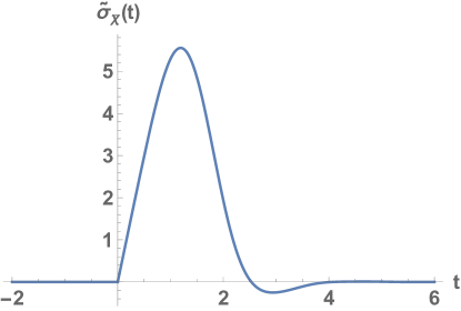
Figure 1: The memory function $\tilde{\sigma}_{\bar{\chi}}(t)$ when $q=0$.

Let us briefly comment on the remaining terms. $\mathcal{D}_{H}$ generalises the Hall diffusion $\mathcal{D}_{H}^{0}$ 1603.03442 ; 1603.03620 ; Bu:2018psl into a TCF of $\omega,q^{2}$; $\bar{\mathcal{D}}_{H}$ is just its axial analogue. So, we will refer to $\mathcal{D}_{H}$ and $\bar{\mathcal{D}}_{H}$ as Hall diffusion functions. $\sigma_{a\chi H}$ is a TCF extending the anomalous chiral Hall conductivity $\sigma_{a\chi H}^{0}$ 1603.03442 ; 1603.03620 ; Bu:2018psl . $\bar{\sigma}_{a\chi H}$ could be considered as an axial analogue of $\sigma_{a\chi H}$. However, as will be clear later, $\bar{\sigma}_{a\chi H}$ has an overall factor $q^{2}$ so that it will be non-vanishing starting from fourth order in the gradient expansion only.

$\sigma_{1,2,3}$ and $\bar{\sigma}_{3}$ are TCFs of the third order derivative operators (we remind the reader that the e/m fields are counted as of first order). $\sigma_{1},\sigma_{2}$ correspond to rotor of Hall diffusion Bu:2018psl , and $\sigma_{3},\bar{\sigma}_{3}$ are rotors of anomalous chiral Hall effect Bu:2018psl .

Each TCF in (7, 8) can be split into real part (even powers of frequency) and imaginary part (odd powers of frequency). Based on the time reversal criterion, we conclude that the real parts of $\sigma_{\bar{\chi},1,2}$, $\mathcal{D}_{H}$, $\bar{\mathcal{D}}_{H}$ and imaginary parts of $\sigma_{a\chi H},\bar{\sigma}_{a\chi H}$,$\sigma_{3},\bar{\sigma}_{3}$ are non-dissipative; all the rest do lead to dissipation of the currents. It is interesting to notice that there are points in the ($\omega,q$) phase space, where some of the dissipative terms vanish. Particularly, this happens to $\rm Re[\mathcal{D}]$ and $\rm Im[\sigma_{\bar{\chi}}]$. This feature leads to presence of a non-dissipative discrete density wave mode which is mentioned earlier.

The constitutive relations (7, 8) could be re-written in a more compact way,

$$\begin{split}J^{(1)(1)}_{i}=&\sigma_{\bar{\chi}}\kappa{\bf B}_{i}\delta\rho_{5}-\kappa{\bf B}_{i}\left(\sigma_{1}\vec{\nabla}^{2}\rho+\sigma_{2}\vec{\nabla}^{2}\rho_{5}\right)-\kappa{\bf E}_{i}\left(\sigma_{3}\vec{\nabla}^{2}\rho+\bar{\sigma}_{3}\vec{\nabla}^{2}\rho_{5}\right)-\mathcal{D}_{ij}^{1}\nabla_{j}\rho\\ &-(\mathcal{D_{\chi}})_{ij}^{1}\nabla_{j}\rho_{5},\end{split}$$ (14)

$$\begin{split}J^{(1)(1)}_{5i}=&\sigma_{\bar{\chi}}\kappa{\bf B}_{i}\delta\rho-\kappa{\bf B}_{i}\left(\sigma_{1}\vec{\nabla}^{2}\rho+\sigma_{2}\vec{\nabla}^{2}\rho_{5}\right)-\kappa{\bf E}_{i}\left(\sigma_{3}\vec{\nabla}^{2}\rho+\bar{\sigma}_{3}\vec{\nabla}^{2}\rho_{5}\right)-\mathcal{D}_{ij}^{1}\nabla_{j}\rho_{5}\\ &-(\mathcal{D_{\chi}})_{ij}^{1}\nabla_{j}\rho,\end{split}$$ (15)

where

$$\mathcal{D}_{ij}^{1} =-\delta_{ij}\kappa\left[\left(\vec{\bf B}\cdot\vec{\nabla}\right)\sigma_{1}+\left(\vec{\bf E}\cdot\vec{\nabla}\right)\sigma_{3}\right]+\frac{1}{4}\epsilon_{ikj}\left(\bar{\rho}\vec{\bf B}_{k}\mathcal{D}_{H}+2\vec{\bf E}_{k}\bar{\sigma}_{a\chi H}\right),$$

$$(\mathcal{D}_{\chi})_{ij}^{1} =-\delta_{ij}\kappa\left[\left(\vec{\bf B}\cdot\vec{\nabla}\right)\sigma_{2}+\left(\vec{\bf E}\cdot\vec{\nabla}\right)\bar{\sigma}_{3}\right]+\frac{1}{4}\epsilon_{ikj}\left(\bar{\rho}_{5}\vec{\bf B}_{k}\bar{\mathcal{D}}_{H}+2\vec{\bf E}_{k}\sigma_{a\chi H}\right).$$ (16)

$\sigma_{1,2,3}$ and $\bar{\sigma}_{3}$ constitute corrections to CME/CSE and, through spatial inhomogeneities of $\rho,\rho_{5}$, influence the Ohmic conductivity. The scalar diffusion function $\mathcal{D}$ 1511.08789 now becomes tensor TCFs $\mathcal{D}_{ij}^{1}$ and $(\mathcal{D}_{\chi})_{ij}^{1}$, linearly depending on $\vec{\bf E}$ and $\vec{\bf B}$ because of the weak field approximation adopted here.

In the hydrodynamic limit $\omega,q\ll 1$, the TCFs in (7, 8) are expandable (below we set $\pi T=1$ for convenience and the dimensionful frequency and momentum are $\pi T\omega$ and $\pi Tq$):

$$\sigma_{\bar{\chi}}=6+\frac{3}{2}i\omega\left(\pi+2\log 2\right)-\frac{1}{8}\left\{\omega^{2}\left[\pi^{2}+6\left(4\mathcal{C}+\log^{2}2\right)\right]+q^{2}\left(12\pi-24\log 2\right)\right\}+\cdots,$$ (17)

$$\mathcal{D}_{H}=\kappa^{2}\left\{72(3\log 2-2)+i\omega 6\left[\pi(2\pi+3\log 2-6)+(9\log 2-12)\log 2\right]+\cdots\right\},$$ (18)

$$\bar{\mathcal{D}}_{H}=\mathcal{D}_{H}\left[\bar{\mu}\leftrightarrow\bar{\mu}_{5}\right],$$ (19)

$$\sigma_{a\chi H}=\kappa\left\{6\log 2+i\omega\frac{1}{16}\left(48\mathcal{C}+5\pi^{2}\right)+\cdots\right\},$$ (20)

$$\bar{\sigma}_{a\chi H}=0+\cdots,$$ (21)

$$\sigma_{1}=162\kappa^{2}\bar{\mu}\bar{\mu}_{5}\left[6+\log 2(5\log 2-12)\right]+\cdots,$$ (22)

$$\sigma_{2}=\frac{1}{8}(6\pi-\pi^{2}-12\log 2)+108\kappa^{2}(\bar{\mu}^{2}+\bar{\mu}_{5}^{2})\left[6+\log 2(5\log 2-12)\right]+\cdots,$$ (23)

$$\sigma_{3}=9\kappa\bar{\mu}\log^{2}2+\cdots,$$ (24)

$$\bar{\sigma}_{3}=\sigma_{3}\left[\bar{\mu}\leftrightarrow\bar{\mu}_{5}\right],$$ (25)

where $\cdots$ denotes higher powers in $\omega,q^{2}$ and $\mathcal{C}\approx 0.915966$ is the Catalan’s constant. Here, $\bar{\mu}=\bar{\rho}/2,\bar{\mu}_{5}=\bar{\rho}_{5}/2$ are backgrounds for vector/axial chemical potentials. While each term in (17-25) have been computed as individual TC in Bu:2018psl , the resummation procedure here collects all relevant TCs into a single TCF and determines the most general structure of currents, valid to all orders.

Beyond the hydrodynamic limit, the TCFs are computed numerically. The results are presented and discussed in subsection IV.3. We observe a relatively weak dependence on $q^{2}$ while $\omega$-dependence is more profound: damped oscillations towards asymptotic regime around $\omega\simeq 5$. We remark that none of the TCFs survives beyond asymptotically large $\omega\gtrsim 5$. For the details about each TCF we refer to subsection IV.3.

It is interesting to explore dependence of the TCFs on the chemical potentials. Of special interest is the case of zero background axial charge density, $\bar{\rho}_{5}=0$, which is the most realistic scenario for any conceivable experiment. However, even in this case, $\mu_{5}$ could be nonzero and would be proportional to $\vec{\bf E}\cdot\vec{\bf B}$ due to the chiral anomaly (1). Because of the linearisation approximation, the TCFs $\sigma_{1},\bar{\sigma}_{3}$ vanish in the limit $\bar{\rho}_{5}=0$. We expect them to be nonzero beyond the current approximation. At $q=0$, for the remaining TCFs we discover some universal dependence: $\bar{\sigma}_{a\chi H}$ vanishes; $\sigma_{a\chi H}$, $\mathcal{D}_{H}$, $\bar{\mathcal{D}}_{H}$ do not depend on the chemical potentials at all; $\sigma_{1}$ is linear in $\kappa^{2}\bar{\mu}\bar{\mu}_{5}$; $\sigma_{3}$ is linear in $\kappa\bar{\mu}$; similarly, $\bar{\sigma}_{3}$ is linear in $\kappa\bar{\mu}_{5}$; $\sigma_{2}$ has a normal component independent of the chemical potentials and anomaly induced correction which is linear in $\kappa^{2}(\bar{\mu}^{2}+\bar{\mu}_{5}^{2})$. All these features can be derived from the underlying equations (see Appendix A.1 for relevant ODEs).

The rest of this paper is structured as follows. In Section III, we present the holographic model briefly. For more details about holographic model we refer to Bu:2018psl . Section IV contains the main part of the study: gradient resummation for nonlinear chiral transport. It is further split into four subsections. In subsection IV.1, the constitutive relations (7,8) are derived from the dynamical components of the bulk anomalous Maxwell equations near the conformal boundary. In subsection IV.2, the TCFs are analytically computed in the hydrodynamic limit. Subsection IV.3 numerically extends the results beyond this limit. Subsection IV.4 focuses on the CMW dispersion relation beyond hydrodynamic limit. Section V concludes our study. Appendices supplement calculational details for Section IV.

III Holographic setup: $U(1)_{V}\times U(1)_{A}$

The bulk action is Yee:2009vw ; Gynther:2010ed

$$S=\int d^{5}x\sqrt{-g}\mathcal{L}+S_{\textrm{c.t.}},$$ (26)

where

$$\begin{split}\mathcal{L}=&-\frac{1}{4}(F^{V})_{MN}(F^{V})^{MN}-\frac{1}{4}(F^{a})_{MN}(F^{a})^{MN}+\frac{\kappa\,\epsilon^{MNPQR}}{2\sqrt{-g}}\\ &\times\left[3A_{M}(F^{V})_{NP}(F^{V})_{QR}+A_{M}(F^{a})_{NP}(F^{a})_{QR}\right],\end{split}$$ (27)

and the counter-term action $S_{\textrm{c.t.}}$ is

$$S_{\textrm{c.t.}}=\frac{1}{4}\log r\int d^{4}x\sqrt{-\gamma}\left[(F^{V})_{\mu\nu}(F^{V})^{\mu\nu}+(F^{a})_{\mu\nu}(F^{a})^{\mu\nu}\right].$$ (28)

The gauge Chern-Simons terms ($\sim\kappa$) in the bulk action mimic the chiral anomaly of the boundary field theory. Note $\epsilon^{MNPQR}$ is the Levi-Civita symbol with the convention $\epsilon^{rtxyz}=+1$, while the Levi-Civita tensor is $\epsilon^{MNPQR}/\sqrt{-g}$.

In the ingoing Eddington-Finkelstein coordinate, the metric of Schwarzschild-$AdS_{5}$ is

$$ds^{2}=2dtdr-r^{2}f(r)dt^{2}+r^{2}\delta_{ij}dx^{i}dx^{j},$$ (29)

where $f(r)=1-1/r^{4}$. Here we have normalised the Hawking temperature (identified as the temperature of the boundary theory) to $\pi T=1$.

The bulk equations of motion read

$$\textrm{EV}^{M}\equiv\nabla_{N}(F^{V})^{NM}+\frac{3\kappa\epsilon^{MNPQR}}{\sqrt{-g}}(F^{a})_{NP}(F^{V})_{QR}=0,$$ (30)

$$\textrm{EA}^{M}\equiv\nabla_{N}(F^{a})^{NM}+\frac{3\kappa\epsilon^{MNPQR}}{2\sqrt{-g}}\left[(F^{V})_{NP}(F^{V})_{QR}+(F^{a})_{NP}(F^{a})_{QR}\right]=0,$$ (31)

where $\textrm{EV}^{\mu}=\textrm{EA}^{\mu}=0$ and $\textrm{EV}^{r}=\textrm{EA}^{r}=0$ correspond to dynamical and constraint equations, respectively. The boundary currents are defined as

$$J^{\mu}\equiv\lim_{r\to\infty}\frac{\delta S}{\delta V_{\mu}},~{}~{}~{}~{}~{}~{}~{}~{}~{}~{}~{}~{}~{}J^{\mu}_{5}\equiv\lim_{r\to\infty}\frac{\delta S}{\delta A_{\mu}}.$$ (32)

Employing the radial gauge $V_{r}=A_{r}=0$, it is sufficient to solve the dynamical equations only to determine the boundary currents (32), leaving constraints aside. Indeed, the constraint equations give rise to continuity equations of currents (1). Thus, without imposing the constraint equations, the currents to be constructed are off-shell.

For practical purpose, it is useful to express the currents in terms of the coefficients of near boundary ($r=\infty$) pre-asymptotic expansion of the bulk gauge fields:

$$\begin{split}J^{\mu}=\eta^{\mu\nu}(2V_{\nu}^{(2)}+2V^{\textrm{L}}_{\nu}+\eta^{\sigma t}\partial_{\sigma}\mathcal{F}_{t\nu}^{V}),\qquad\qquad J_{5}^{\mu}=\eta^{\mu\nu}2A_{\nu}^{(2)},\end{split}$$ (33)

where $\mathcal{F}_{\mu\nu}^{V}$ is field strength of the external e/m potential $\mathcal{V}_{\mu}(x)$, and $4V_{\mu}^{\textrm{L}}=\partial^{\nu}\mathcal{F}_{\mu\nu}^{V}$. $V_{\mu}^{(2)}$ and $A_{\mu}^{(2)}$ are the coefficients of $1/r^{2}$ in the near boundary expansions of bulk fields $V_{\mu}$ and $A_{\mu}$, respectively. Note $V_{\mu}^{(2)}$ and $A_{\mu}^{(2)}$ have to be determined by fully solving the dynamical equations from the horizon to the boundary.

As the remainder of this section, we outline the strategy for deriving the constitutive relations for $J^{\mu}$ and $J_{5}^{\mu}$. To this end, we turn on finite vector/axial charge densities for the dual field theory, which are also exposed to external e/m fields $\mathcal{V}_{\mu}$. Holographically, the charge densities and external fields are encoded in the asymptotic behaviors of the bulk gauge fields. In the bulk, we will solve the dynamical equations assuming the charge densities and external fields as given, but without specifying them explicitly. For more details, we refer the reader to our previous publications 1608.08595 ; 1609.09054 ; Bu:2018psl .

We start with the ansatz

$$\begin{split}V_{\mu}(r,x_{\alpha})=\mathcal{V}_{\mu}(x_{\alpha})-\frac{\rho(x_{\alpha})}{2r^{2}}\delta_{\mu t}+\mathbb{V}_{\mu}(r,x_{\alpha}),\qquad A_{\mu}(r,x_{\alpha})=-\frac{\rho_{{}_{5}}(x_{\alpha})}{2r^{2}}\delta_{\mu t}+\mathbb{A}_{\mu}(r,x_{\alpha}),\end{split}$$ (34)

where $\mathcal{V}_{\mu}(x)$ is the external gauge potential, and $\rho,\rho_{5}$ are vector and axial charge densities of the boundary theory. $\mathbb{V}_{\mu}$ and $\mathbb{A}_{\mu}$ will be determined by solving dynamical equations. Appropriate boundary conditions are classified into three types. First, $\mathbb{V}_{\mu}$ and $\mathbb{A}_{\mu}$ are regular over the domain $r\in[1,\infty)$. Second, at the conformal boundary $r=\infty$, we require

$$\mathbb{V}_{\mu}\to 0,~{}~{}~{}~{}~{}~{}\mathbb{A}_{\mu}\to 0~{}~{}~{}~{}~{}~{}~{}\textrm{as}~{}~{}~{}~{}~{}~{}r\to\infty,$$ (35)

which amounts to fixing external gauge potentials to be $\mathcal{V}_{\mu}$ and zero (for the axial field). Additional integration constants will be fixed by the Landau frame convention,

$$J^{t}=\rho(x_{\alpha}),~{}~{}~{}~{}~{}~{}~{}~{}~{}~{}~{}J^{t}_{5}=\rho_{{}_{5}}(x_{\alpha}).$$ (36)

The Landau frame convention corresponds to a residual gauge fixing for the bulk fields.

To facilitate the exchange between charge density and chemical potential, we define

$$\begin{split}\mu&=V_{t}(r=\infty)-V_{t}(r=1)=\frac{1}{2}\rho-\mathbb{V}_{t}(r=1),\\ \mu_{{}_{5}}&=A_{t}(r=\infty)-A_{t}(r=1)=\frac{1}{2}\rho_{{}_{5}}-\mathbb{A}_{t}(r=1).\end{split}$$ (37)

Generically, $\mu,\mu_{{}_{5}}$ are nonlinear functionals of densities and external fields.

For generic profiles of $\mathcal{V}_{\mu}(x),\rho(x),\rho_{5}(x)$, it is impossible to solve dynamical components of (30, 31). As announced in section III, we employ the approximation schemes (4 ,5). Consequently, the corrections $\mathbb{V}_{\mu}$ and $\mathbb{A}_{\mu}$ are first expanded in powers of $\epsilon$,

$$\mathbb{V}_{\mu}=\mathbb{V}_{\mu}^{(0)}(r)+\epsilon\mathbb{V}_{\mu}^{(1)}(r,x^{\alpha})+\mathcal{O}(\epsilon^{2}),\qquad\qquad\mathbb{A}_{\mu}=\mathbb{A}_{\mu}^{(0)}(r)+\epsilon\mathbb{A}_{\mu}^{(1)}(r,x^{\alpha})+\mathcal{O}(\epsilon^{2}),$$ (38)

and then each order in $\epsilon$ is further expanded in powers of $\alpha$:

$$\begin{split}&\mathbb{V}_{\mu}^{(0)}=\sum^{\infty}_{n=1}\alpha^{n}\mathbb{V}^{(0)(n)}_{\mu},\qquad\qquad\mathbb{A}_{\mu}^{(0)}=\sum^{\infty}_{n=1}\alpha^{n}\mathbb{A}^{(0)(n)}_{\mu},\\ &\mathbb{V}_{\mu}^{(1)}=\sum^{\infty}_{n=0}\alpha^{n}\mathbb{V}^{(1)(n)}_{\mu},\qquad\qquad\mathbb{A}_{\mu}^{(1)}=\sum^{\infty}_{n=0}\alpha^{n}\mathbb{A}^{(1)(n)}_{\mu},\end{split}$$ (39)

where $\mathbb{V}_{\mu}^{(0)(1)}$, $\mathbb{V}_{\mu}^{(1)(0)}$, $\mathbb{A}_{\mu}^{(0)(1)}$, $\mathbb{A}_{\mu}^{(1)(0)}$ were derived in 1608.08595 . Since $\mathbb{V}_{\mu}^{(0)(1)}$, $\mathbb{V}_{\mu}^{(1)(0)}$, $\mathbb{A}_{\mu}^{(0)(1)}$, $\mathbb{A}_{\mu}^{(1)(0)}$ will act as sources in the dynamical equations at $\mathcal{O}(\epsilon^{1}\alpha^{1})$, we summarise them below (the notations here will be slightly different from 1608.08595 ).

At $\mathcal{O}(\epsilon^{0}\alpha^{1})$, we have

$$\mathbb{V}^{(0)(1)}_{t}=\mathbb{A}^{(0)(1)}_{t}=0,\qquad\mathbb{V}^{(0)(1)}_{i}=f_{1}\mathbf{E}_{i}+f_{2}\kappa\bar{\rho}_{5}\mathbf{B}_{i},\qquad\mathbb{A}^{(0)(1)}_{i}=f_{2}\kappa\bar{\rho}\mathbf{B}_{i},$$ (40)

where $f_{1}$ and $f_{2}$ are 1608.08595

$$f_{1}=-\frac{1}{4}\left[\log\frac{(1+r)^{2}}{1+r^{2}}-2\arctan(r)+\pi\right]\qquad\text{and}\qquad f_{2}=3\log\frac{1+r^{2}}{r^{2}}.$$ (41)

At $\mathcal{O}(\epsilon^{1}\alpha^{0})$, the corrections are (note $\delta\vec{E}=\delta\vec{B}=0$ throughout this work)

$$\begin{split}&\mathbb{V}^{(1)(0)}_{t}=g_{3}(r,\omega,\vec{q}\,)\delta\rho,~{}~{}~{}~{}~{}~{}~{}~{}~{}~{}~{}~{}~{}~{}~{}~{}~{}~{}~{}~{}~{}~{}~{}~{}~{}~{}~{}~{}\mathbb{A}^{(1)(0)}_{t}=g_{3}(r,\omega,\vec{q}\,)\delta\rho_{5},\\ &\mathbb{V}^{(1)(0)}_{i}=g_{4}(r,\omega,\vec{q}\,)\partial_{i}\delta\rho,~{}~{}~{}~{}~{}~{}~{}~{}~{}~{}~{}~{}~{}~{}~{}~{}~{}~{}~{}~{}~{}~{}~{}~{}~{}~{}\mathbb{A}^{(1)(0)}_{i}=g_{4}(r,\omega,\vec{q}\,)\partial_{i}\delta\rho_{5}.\end{split}$$ (42)

$g_{3}$ and $g_{4}$ satisfy coupled ordinary differential equations (ODEs),

$$\begin{split}&0=r^{2}\partial^{2}_{r}g_{3}+3r\partial_{r}g_{3}-q^{2}\partial_{r}g_{4},\\ &0=(r^{5}-r)\partial^{2}_{r}g_{4}+(3r^{4}+1)\partial_{r}g_{4}-2i\omega r^{3}\partial_{r}g_{4}-i\omega r^{2}g_{4}-r^{3}\partial_{r}g_{3}-r^{2}g_{3}-\frac{1}{2},\end{split}$$ (43)

which were solved both analytically in the hydro limit ($\omega,q\ll 1$) and numerically for generic values of $\omega,q$ in Ref. 1608.08595 . Below we quote the hydro expansion of diffusion function $\mathcal{D}$ 1511.08789 (which can be extracted from solution to $g_{4}$):

$$\mathcal{D}=\frac{1}{2}+\frac{i\omega\pi}{8}-\frac{1}{48}\left[\pi^{2}\omega^{2}-q^{2}(6\log 2-3\pi)\right]+\cdots,$$ (44)

At $\mathcal{O}(\epsilon^{1}\alpha^{1})$, the dynamical equations reduce to the following linear partial differential equations for the corrections $\mathbb{V}_{\mu}^{(1)(1)}$ and $\mathbb{A}_{\mu}^{(1)(1)}$:

$$\begin{split}0&=r^{3}\partial_{r}^{2}\mathbb{V}^{(1)(1)}_{t}+3r^{2}\partial_{r}\mathbb{V}^{(1)(1)}_{t}+r\partial_{r}\partial_{k}\mathbb{V}^{(1)(1)}_{k}+12\kappa\epsilon^{ijk}\left(\partial_{r}\mathbb{A}^{(1)(0)}_{i}\partial_{j}\bar{\mathcal{V}}_{k}\right.\\ &\left.+\partial_{r}\mathbb{A}^{(0)(1)}_{i}\partial_{j}\mathbb{V}^{(1)(0)}_{k}+\partial_{r}\mathbb{V}^{(0)(1)}_{i}\partial_{j}\mathbb{A}^{(1)(0)}_{k}\right),\end{split}$$ (45)

$$\begin{split}0&=(r^{5}-r)\partial^{2}_{r}\mathbb{V}^{(1)(1)}_{i}+(3r^{4}+1)\partial_{r}\mathbb{V}^{(1)(1)}_{i}+2r^{3}\partial_{r}\partial_{t}\mathbb{V}_{i}^{(1)(1)}-r^{3}\partial_{r}\partial_{i}\mathbb{V}^{(1)(1)}_{t}\\ &+r^{2}\left(\partial_{t}\mathbb{V}^{(1)(1)}_{i}-\partial_{i}\mathbb{V}^{(1)(1)}_{t}\right)+r\left(\partial^{2}\mathbb{V}^{(1)(1)}_{i}-\partial_{i}\partial_{k}\mathbb{V}^{(1)(1)}_{k}\right)+12\kappa r^{2}\epsilon^{ijk}\\ &\times\left(\frac{1}{r^{3}}\delta\rho_{5}\partial_{j}\bar{\mathcal{V}}_{k}+\frac{1}{r^{3}}\bar{\rho}_{5}\partial_{j}\mathbb{V}^{(1)(1)}_{k}+\partial_{r}\mathbb{A}^{(1)(0)}_{t}\partial_{j}\bar{\mathcal{V}}_{k}\right)-12\kappa r^{2}\epsilon^{ijk}\\ &\times\left\{\partial_{r}\mathbb{A}^{(0)(1)}_{j}\left[(\partial_{t}\mathbb{V}^{(1)(0)}_{k}-\partial_{k}\mathbb{V}^{(1)(0)}_{t})+\frac{1}{2r^{2}}\partial_{k}\delta\rho\right]+\partial_{r}\mathbb{A}^{(1)(0)}_{j}\left(\partial_{t}\bar{\mathcal{V}}_{k}-\partial_{k}\bar{\mathcal{V}}_{t}\right)\right\}\\ &-12\kappa r^{2}\epsilon^{ijk}\left\{\partial_{r}\mathbb{V}^{(0)(1)}_{j}\left[(\partial_{t}\mathbb{A}^{(1)(0)}_{k}-\partial_{k}\mathbb{A}^{(1)(0)}_{t})+\frac{1}{2r^{2}}\partial_{k}\delta\rho_{5}\right]-\frac{\bar{\rho}}{r^{3}}\partial_{j}\mathbb{A}^{(1)(1)}_{k}\right\},\end{split}$$ (46)

$$\begin{split}0&=r^{3}\partial_{r}^{2}\mathbb{A}^{(1)(1)}_{t}+3r^{2}\partial_{r}\mathbb{A}^{(1)(1)}_{t}+r\partial_{r}\partial_{k}\mathbb{A}^{(1)(1)}_{k}+12\kappa\epsilon^{ijk}\left(\partial_{r}\mathbb{V}^{(1)(0)}_{i}\partial_{j}\bar{\mathcal{V}}_{k}\right.\\ &\left.+\partial_{r}\mathbb{V}^{(0)(1)}_{i}\partial_{j}\mathbb{V}^{(1)(0)}_{k}+\partial_{r}\mathbb{A}^{(0)(1)}_{i}\partial_{j}\mathbb{A}^{(1)(0)}_{k}\right),\end{split}$$ (47)

$$\begin{split}0&=(r^{5}-r)\partial_{r}^{2}\mathbb{A}^{(1)(1)}_{i}+(3r^{4}+1)\partial_{r}\mathbb{A}^{(1)(1)}_{i}+2r^{3}\partial_{r}\partial_{t}\mathbb{A}^{(1)(1)}_{i}-r^{3}\partial_{r}\partial_{i}\mathbb{A}^{(1)(1)}_{t}\\ &+r^{2}\left(\partial_{t}\mathbb{A}^{(1)(1)}_{i}-\partial_{i}\mathbb{A}^{(1)(1)}_{t}\right)+r\left(\partial^{2}\mathbb{A}^{(1)(1)}_{i}-\partial_{i}\partial_{k}\mathbb{A}^{(1)(1)}_{k}\right)+12\kappa r^{2}\epsilon^{ijk}\\ &\times\left(\partial_{j}\bar{\mathcal{V}}_{k}(\partial_{r}\mathbb{V}^{(1)(0)}_{t}+\frac{1}{r^{3}}\delta\rho)+\frac{\bar{\rho}}{r^{3}}\partial_{j}\mathbb{V}^{(1)(1)}_{k}\right)-12\kappa r^{2}\epsilon^{ijk}\\ &\times\left\{\partial_{r}\mathbb{V}^{(0)(1)}_{j}\left[(\partial_{t}\mathbb{V}^{(1)(0)}_{k}-\partial_{k}\mathbb{V}_{t}^{(1)(0)})+\frac{1}{2r^{2}}\partial_{k}\delta\rho\right]+\partial_{r}\mathbb{V}^{(1)(0)}_{j}(\partial_{t}\bar{\mathcal{V}}_{k}-\partial_{k}\bar{\mathcal{V}}_{t})\right\}\\ &-12\kappa r^{2}\epsilon^{ijk}\left\{\partial_{r}\mathbb{A}^{(0)(1)}_{j}\left[(\partial_{t}\mathbb{A}^{(1)(0)}_{k}-\partial_{k}\mathbb{A}^{(1)(0)}_{t})+\frac{1}{2r^{2}}\partial_{k}\delta\rho_{5}\right]-\frac{\bar{\rho_{5}}}{r^{3}}\partial_{j}\mathbb{A}^{(1)(1)}_{k}\right\}.\end{split}$$ (48)

In the next section IV, we will solve (45-48) by the technique invented in 1406.7222 ; 1409.3095 .

IV Nonlinear chiral transport and gradient resummation

In this section, we focus on all order gradient resummation. It is split into four subsections. The first one IV.1 is devoted to derivation of the constitutive relations (7, 8). In the following subsections IV.2 and IV.3, the TCFs in (7, 8) are evaluated, first analytically in the hydrodynamic limit, and then numerically for arbitrary momenta. The last subsection IV.4 is about non-dissipative modes in the CMW dispersion relations.

IV.1 Constitutive relations at $\mathcal{O}(\epsilon^{1}\alpha^{1})$

Following the formalism introduced in 1406.7222 ; 1409.3095 , the corrections $\mathbb{V}_{\mu}^{(1)(1)}$ and $\mathbb{A}_{\mu}^{(1)(1)}$ are decomposed in terms of basic structures built from the external fields and inhomogeneous parts of the charge densities,

$$\mathbb{V}^{(1)(1)}_{t}=S_{1}\kappa\mathbf{B}_{k}\partial_{k}\delta\rho+S_{2}\kappa\mathbf{E}_{k}\partial_{k}\delta\rho+S_{3}\kappa\mathbf{B}_{k}\partial_{k}\delta\rho_{5}+S_{4}\kappa\mathbf{E}_{k}\partial_{k}\delta\rho_{5},$$ (49)

$$\begin{split}\mathbb{V}^{(1)(1)}_{i}&=V_{1}\kappa\mathbf{B}_{i}\delta\rho+V_{2}\kappa\mathbf{B}_{k}\partial_{i}\partial_{k}\delta\rho+V_{3}\kappa\epsilon^{ijk}\mathbf{B}_{j}\partial_{k}\delta\rho+V_{4}\kappa\mathbf{E}_{i}\delta\rho+V_{5}\kappa\mathbf{E}_{k}\partial_{i}\partial_{k}\delta\rho,\\ &+V_{6}\kappa\epsilon^{ijk}\mathbf{E}_{j}\partial_{k}\delta\rho+V_{7}\kappa\mathbf{B}_{i}\delta\rho_{5}+V_{8}\kappa\mathbf{B}_{k}\partial_{i}\partial_{k}\delta\rho_{5}+V_{9}\kappa\epsilon^{ijk}\mathbf{B}_{j}\partial_{k}\delta\rho_{5}+V_{10}\kappa\mathbf{E}_{i}\delta\rho_{5}\\ &+V_{11}\kappa\mathbf{E}_{k}\partial_{i}\partial_{k}\delta\rho_{5}+V_{12}\kappa\epsilon^{ijk}\mathbf{E}_{j}\partial_{k}\delta\rho_{5},\end{split}$$ (50)

$$\mathbb{A}^{(1)(1)}_{t}=\bar{S}_{1}\kappa\mathbf{B}_{k}\partial_{k}\delta\rho+\bar{S}_{2}\kappa\mathbf{E}_{k}\partial_{k}\delta\rho+\bar{S}_{3}\kappa\mathbf{B}_{k}\partial_{k}\delta\rho_{5}+\bar{S}_{4}\kappa\mathbf{E}_{k}\partial_{k}\delta\rho_{5},$$ (51)

$$\begin{split}\mathbb{A}^{(1)(1)}_{i}&=\bar{V}_{1}\kappa\mathbf{B}_{i}\delta\rho+\bar{V}_{2}\kappa\mathbf{B}_{k}\partial_{i}\partial_{k}\delta\rho+\bar{V}_{3}\kappa\epsilon^{ijk}\mathbf{B}_{j}\partial_{k}\delta\rho+\bar{V}_{4}\kappa\mathbf{E}_{i}\delta\rho+\bar{V}_{5}\kappa\mathbf{E}_{k}\partial_{i}\partial_{k}\delta\rho\\ &+\bar{V}_{6}\kappa\epsilon^{ijk}\mathbf{E}_{j}\partial_{k}\delta\rho+\bar{V}_{7}\kappa\mathbf{B}_{i}\delta\rho_{5}+\bar{V}_{8}\kappa\mathbf{B}_{k}\partial_{i}\partial_{k}\delta\rho_{5}+\bar{V}_{9}\kappa\epsilon^{ijk}\mathbf{B}_{j}\partial_{k}\delta\rho_{5}+\bar{V}_{10}\kappa\mathbf{E}_{i}\delta\rho_{5}\\ &+\bar{V}_{11}\kappa\mathbf{E}_{k}\partial_{i}\partial_{k}\delta\rho_{5}+\bar{V}_{12}\kappa\epsilon^{ijk}\mathbf{E}_{j}\partial_{k}\delta\rho_{5},\end{split}$$ (52)

where $S_{i}$, $\bar{S}_{i}$, $V_{i}$ and $\bar{V}_{i}$ are functionals of the boundary derivative operator $\partial_{\mu}$ and functions of the radial coordinate $r$. They also depend on the constant values $\bar{\mu}$ and $\bar{\mu}_{5}$ of the chemical potentials. Fourier transforming $\delta\rho$ and $\delta\rho_{5}$ turns all the derivatives into momenta. Thus, in momentum space, these decomposition coefficients become functions of the radial coordinate, frequency $\omega$ and spatial momentum squared $q^{2}$:

$$S_{i}\left(r,\partial_{t},\partial_{i}^{2}\right)\rightarrow S_{i}\left(r,\omega,q^{2}\right)\qquad\qquad\bar{S}_{i}\left(r,\partial_{t},\partial_{i}^{2}\right)\rightarrow\bar{S}_{i}\left(r,\omega,q^{2}\right),$$ (53)

$$V_{i}\left(r,\partial_{t},\partial_{i}^{2}\right)\rightarrow V_{i}\left(r,\omega,q^{2}\right)\qquad\qquad\bar{V}_{i}\left(r,\partial_{t},\partial_{i}^{2}\right)\rightarrow\bar{V}_{i}\left(r,\omega,q^{2}\right),$$ (54)

which satisfy partially decoupled inhomogeneous ODEs listed in Appendix-A.1. The decomposition functions $S_{i}$, $\bar{S}_{i}$, $V_{i}$ and $\bar{V}_{i}$ are nothing else but elements of the inverse Green function matrix for the system of ODEs.

As discussed in Section III, the boundary conditions for the decomposition coefficients in (49-52) are

$$S_{i}\rightarrow 0,\qquad\quad\bar{S}_{i}\rightarrow 0\qquad\quad V_{i}\rightarrow 0,\qquad\quad\bar{V}_{i}\rightarrow 0\qquad\qquad\text{as}\qquad r\rightarrow\infty.$$ (55)

$$S_{i},\quad\bar{S}_{i},\quad V_{i},\quad\bar{V}_{i}\qquad\text{are regular over the whole integral of}~{}r\in[1,\infty).$$ (56)

Additional integration constants will be fixed by the Landau frame convention (36).

Solving the ODEs (73-88) near the boundary $r=\infty$ reveals the pre-asymptotic behaviour for the corrections, which can be summarised as

$$\begin{split}S_{i}\rightarrow\frac{s_{i}^{1}}{r}+\frac{s_{i}}{r^{2}}+\frac{s_{i}^{\rm L}\log r}{r^{2}}+\cdots,\qquad\quad\quad V_{i}\rightarrow\frac{v_{i}^{1}}{r}+\frac{v_{i}}{r^{2}}+\frac{v_{i}^{\rm L}\log r}{r^{2}}+\cdots,\\ \bar{S}_{i}\rightarrow\frac{\bar{s}_{i}^{1}}{r}+\frac{\bar{s}_{i}}{r^{2}}+\frac{\bar{s}_{i}^{\rm L}\log r}{r^{2}}+\cdots,\qquad\quad\quad\bar{V}_{i}\rightarrow\frac{\bar{v}_{i}^{1}}{r}+\frac{\bar{v}_{i}}{r^{2}}+\frac{\bar{v}_{i}^{\rm L}\log r}{r^{2}}+\cdots,\end{split}$$ (57)

where $s_{i}^{1,{\rm L}}$, $v_{i}^{1,{\rm L}}$, $\bar{s}_{i}^{1,{\rm L}}$, $\bar{v}_{i}^{1,{\rm L}}$ are fixed uniquely from the near-boundary analysis alone, while the coefficients $s_{i}$, $v_{i}$, $\bar{s}_{i}$, $\bar{v}_{i}$ can be determined only when the ODEs are fully solved in the entire bulk, from the horizon to the $AdS$ boundary.

Then, at $\mathcal{O}(\epsilon^{1}\alpha^{1})$ the boundary currents (33) are

$$J^{t(1)(1)}=-2\kappa\left(s_{1}\mathbf{B}_{k}\partial_{k}\delta\rho+s_{2}\mathbf{E}_{k}\partial_{k}\delta\rho+s_{3}\mathbf{B}_{k}\partial_{k}\delta\rho_{5}+s_{4}\mathbf{E}_{k}\partial_{k}\delta\rho_{5}\right),$$ (58)

$$\begin{split}J^{i(1)(1)}&=2\kappa\left(v_{1}\mathbf{B}_{i}\delta\rho+v_{2}\mathbf{B}_{k}\partial_{i}\partial_{k}\delta\rho+v_{3}\epsilon^{ijk}\mathbf{B}_{j}\partial_{k}\delta\rho+v_{4}\mathbf{E}_{i}\delta\rho+v_{5}\mathbf{E}_{k}\partial_{i}\partial_{k}\delta\rho\right.\\ &\left.+v_{6}\epsilon^{ijk}\mathbf{E}_{j}\partial_{k}\delta\rho+v_{7}\mathbf{B}_{i}\delta\rho_{5}+v_{8}\mathbf{B}_{k}\partial_{i}\partial_{k}\delta\rho_{5}+v_{9}\epsilon^{ijk}\mathbf{B}_{j}\partial_{k}\delta\rho_{5}+v_{10}\mathbf{E}_{i}\delta\rho_{5}\right.\\ &\left.+v_{11}\mathbf{E}_{k}\partial_{i}\partial_{k}\delta\rho_{5}+v_{12}\epsilon^{ijk}\mathbf{E}_{j}\partial_{k}\delta\rho_{5}\right),\end{split}$$ (59)

$$J_{5}^{t(1)(1)}=-2\kappa\left(\bar{s}_{1}\mathbf{B}_{k}\partial_{k}\delta\rho+\bar{s}_{2}\mathbf{E}_{k}\partial_{k}\delta\rho+\bar{s}_{3}\mathbf{B}_{k}\partial_{k}\delta\rho_{5}+\bar{s}_{4}\mathbf{E}_{k}\partial_{k}\delta\rho_{5}\right),$$ (60)

$$\begin{split}J_{5}^{i(1)(1)}&=2\kappa\left(\bar{v}_{1}\mathbf{B}_{i}\delta\rho+\bar{v}_{2}\mathbf{B}_{k}\partial_{i}\partial_{k}\delta\rho+\bar{v}_{3}\epsilon^{ijk}\mathbf{B}_{j}\partial_{k}\delta\rho+\bar{v}_{4}\mathbf{E}_{i}\delta\rho+\bar{v}_{5}\mathbf{E}_{k}\partial_{i}\partial_{k}\delta\rho\right.\\ &\left.+\bar{v}_{6}\epsilon^{ijk}\mathbf{E}_{j}\partial_{k}\delta\rho+\bar{v}_{7}\mathbf{B}_{i}\delta\rho_{5}+\bar{v}_{8}\mathbf{B}_{k}\partial_{i}\partial_{k}\delta\rho_{5}+\bar{v}_{9}\epsilon^{ijk}\mathbf{B}_{j}\partial_{k}\delta\rho_{5}+\bar{v}_{10}\mathbf{E}_{i}\delta\rho_{5}\right.\\ &\left.+\bar{v}_{11}\mathbf{E}_{k}\partial_{i}\partial_{k}\delta\rho_{5}+\bar{v}_{12}\epsilon^{ijk}\mathbf{E}_{j}\partial_{k}\delta\rho_{5}\right).\end{split}$$ (61)

The Landau frame convention (36) implies

$$s_{i}=\bar{s}_{i}=0,~{}~{}~{}~{}~{}~{}~{}i=1,2,3,4.$$ (62)

Combined with the ODEs (73, 88), (62) leads to constraints among the decomposition coefficients in (49-52), see (89, 90, 91). Helped by these constraints, (59, 61) can be eventually put into compact form (7, 8). All the TCFs can be identified with the near boundary data $v_{i},\bar{v}_{i}$:

$$\sigma_{\bar{\chi}}=2\left(\bar{v}_{1}-q^{2}\bar{v}_{2}\right),\qquad-\frac{\bar{\rho}}{4\kappa}\mathcal{D}_{H}=2v_{3}=2\bar{v}_{9},\qquad-\frac{\bar{\rho}_{5}}{4\kappa}\bar{\mathcal{D}}_{H}=2v_{9}=2\bar{v}_{3},$$

$$-\frac{1}{2\kappa}\sigma_{a\chi H}=2v_{12}=2\bar{v}_{6},\qquad-\frac{1}{2\kappa}\bar{\sigma}_{a\chi H}=2v_{6}=2\bar{v}_{12},\qquad\sigma_{1}=2v_{2}=2\bar{v}_{8},$$

$$\sigma_{2}=2v_{8}=2\bar{v}_{2},\qquad\sigma_{3}=2v_{5}=2\bar{v}_{11},\qquad\bar{\sigma}_{3}=2v_{11}=2\bar{v}_{5}.$$ (63)

The TCF $\sigma_{\bar{\chi}}$ does not depend on $\bar{\mu},\bar{\mu}_{5}$ at all. The rest of the TCFs bear reminiscence of the axial symmetry. It get reflected in some mirror symmetries with respect to exchange of $\bar{\rho}$ and ${\bar{\rho}}_{5}$ (or equivalently of $\bar{\mu}\leftrightarrow\bar{\mu}_{5}$). We found some “symmetric relations” among the decomposition coefficients in (49-52), see (92, 93). Consequently, the TCFs satisfy

$$\sigma_{1,2}\left[\bar{\mu},\bar{\mu}_{5}\right]=\sigma_{1,2}\left[\bar{\mu}_{5},\bar{\mu}\right],\qquad\sigma_{a\chi H}\left[\bar{\mu},\bar{\mu}_{5}\right]=\sigma_{a\chi H}\left[\bar{\mu}_{5},\bar{\mu}\right],\qquad\bar{\sigma}_{a\chi H}\left[\bar{\mu},\bar{\mu}_{5}\right]=\bar{\sigma}_{a\chi H}\left[\bar{\mu}_{5},\bar{\mu}\right],$$

$$\bar{\mathcal{D}}_{H}[\bar{\mu},\bar{\mu}_{5}]=\mathcal{D}_{H}[\bar{\mu},\bar{\mu}_{5}]|_{\bar{\mu}\leftrightarrow\bar{\mu}_{5}},\qquad\bar{\sigma}_{3}[\bar{\mu},\bar{\mu}_{5}]=\sigma_{3}[\bar{\mu},\bar{\mu}_{5}]|_{\bar{\mu}\leftrightarrow\bar{\mu}_{5}}.$$ (64)

Instead of the charge densities $\rho,\rho_{5}$, chemical potentials are frequently used as hydrodynamic variables to parameterise the currents’ constitutive relations. Up to $\mathcal{O}(\epsilon^{1}\alpha^{1})$, the chemical potentials defined in (37) are

$$\begin{split}&\mu=\frac{1}{2}\rho(x_{\alpha})-\left[g_{3}(r=1)\delta\rho+\kappa\bar{S}_{1}(r=1)\mathbf{B}_{k}\partial_{k}\delta\rho_{5}\right],\\ &\mu_{5}=\frac{1}{2}\rho_{5}(x_{\alpha})-\left[g_{3}(r=1)\delta\rho_{5}+\kappa\bar{S}_{1}(r=1)\mathbf{B}_{k}\partial_{k}\delta\rho\right],\end{split}$$ (65)

where $g_{3}(r=1)$ and $\bar{S}_{1}(r=1)$ denote horizon values of $g_{3}$ (appearing in (42)) and $\bar{S}_{1}$, respectively. Then, (65) can be inverted

$$\rho=\frac{1}{\frac{1}{2}-g_{3}(r=1)}\mu+\frac{\kappa\bar{S}_{1}(r=1)B_{k}\partial_{k}}{\left[\frac{1}{2}-g_{3}(r=1)\right]^{2}}\mu_{5},\qquad\qquad\rho_{5}=\frac{1}{\frac{1}{2}-g_{3}(r=1)}\mu_{5}+\frac{\kappa\bar{S}_{1}(r=1)B_{k}\partial_{k}}{\left[\frac{1}{2}-g_{3}(r=1)\right]^{2}}\mu,$$ (66)

where we have utilised the fact that $g_{3}$ has non-vanishing value starting from second order in the gradient counting. After some manipulations, the currents (7, 8) turn into

$$\vec{J}^{\;(1)(1)}= \sigma_{\bar{\chi}}^{\prime}\kappa\vec{\bf{B}}\delta\mu_{5}-\frac{1}{4}\mathcal{D}_{H}^{\prime}(\bar{\rho}\vec{\bf{B}}\times\vec{\nabla}\delta\mu)-\frac{1}{4}\bar{\mathcal{D}}_{H}^{\prime}(\bar{\rho}_{5}\vec{\bf{B}}\times\vec{\nabla}\delta\mu_{5})-\frac{1}{2}\sigma_{a\chi H}^{\prime}(\vec{\bf{E}}\times\vec{\nabla}\delta\mu_{5})$$ (67)

$$-\frac{1}{2}\bar{\sigma}_{a\chi H}^{\prime}(\vec{\bf{E}}\times\vec{\nabla}\delta\mu)+\sigma_{1}^{\prime}\kappa\left[(\vec{\bf{B}}\times\vec{\nabla})\times\vec{\nabla}\right]\delta\mu++\sigma_{2}^{\prime}\kappa\left[(\vec{\bf{B}}\times\vec{\nabla})\times\vec{\nabla}\right]\delta\mu_{5}$$

$$+\sigma_{3}^{\prime}\kappa\left[(\vec{\bf{E}}\times\vec{\nabla})\times\vec{\nabla}\right]\delta\mu+\bar{\sigma}_{3}^{\prime}\kappa\left[(\vec{\bf{E}}\times\vec{\nabla})\times\vec{\nabla}\right]\delta\mu_{5},$$

$$\vec{J}_{5}^{\;(1)(1)}= \sigma_{\bar{\chi}}^{\prime}\kappa\vec{\bf{B}}\delta\mu-\frac{1}{4}\mathcal{D}_{H}^{\prime}(\bar{\rho}\vec{\bf{B}}\times\vec{\nabla}\delta\mu_{5})-\frac{1}{4}\bar{\mathcal{D}}_{H}^{\prime}(\bar{\rho}_{5}\vec{\bf{B}}\times\vec{\nabla}\delta\mu)-\frac{1}{2}\sigma_{a\chi H}^{\prime}(\vec{\bf{E}}\times\vec{\nabla}\delta\mu)$$ (68)

$$-\frac{1}{2}\bar{\sigma}_{a\chi H}^{\prime}(\vec{\bf{E}}\times\vec{\nabla}\delta\mu_{5})+\sigma_{1}^{\prime}\kappa\left[(\vec{\bf{B}}\times\vec{\nabla})\times\vec{\nabla}\right]\delta\mu_{5}+\sigma_{2}^{\prime}\kappa\left[(\vec{\bf{B}}\times\vec{\nabla})\times\vec{\nabla}\right]\delta\mu_{5}$$

$$+\sigma_{3}^{\prime}\kappa\left[(\vec{\bf{E}}\times\vec{\nabla})\times\vec{\nabla}\right]\delta\mu+\bar{\sigma}_{3}^{\prime}\kappa\left[(\vec{\bf{E}}\times\vec{\nabla})\times\vec{\nabla}\right]\delta\mu,$$

where the TCFs with prime are related to those in (7, 8) by

$$\sigma^{\prime}_{\bar{\chi}}=\frac{\sigma_{\bar{\chi}}}{\frac{1}{2}-g_{3}(r=1)},$$ (69)

and similar equations for the rest.

IV.2 Hydrodynamic expansion: analytical results

In the hydrodynamic limit $\omega,q\ll 1$, the ODEs (73-88) can be solved perturbatively. We employ the expansion parameter $\lambda$ via $\left(\omega,\vec{q}\right)\to\left(\lambda\omega,\lambda\vec{q}\right)$. Then, the decomposition coefficients are expanded in powers of $\lambda$,

$$\begin{split}S_{i}=\sum^{\infty}_{n=0}\lambda^{n}S_{i}^{(n)},\qquad\qquad\qquad\qquad V_{i}=\sum^{\infty}_{n=0}\lambda^{n}V_{i}^{(n)},\\ \bar{S}_{i}=\sum^{\infty}_{n=0}\lambda^{n}\bar{S}_{i}^{(n)},\qquad\qquad\qquad\qquad\bar{V}_{i}=\sum^{\infty}_{n=0}\lambda^{n}\bar{V}_{i}^{(n)}.\end{split}$$ (70)

Then, at each order in $\lambda$, the solutions are expressed as double integrals over $r$, see Appendix-A.2. The hydrodynamic expansions of $v_{i}$ and $\bar{v}_{i}$ (57) can be directly read off from (94-115). Plugging these results into (IV.1) leads to the hydrodynamic expansion of all the TCFs in (7, 8), as presented in (17-25).

IV.3 Beyond the hydrodynamic limit: numerical results

In this section, we present our results for the TCFs in (7, 8) for finite frequency/momentum via solving the ODEs (73-88) numerically. Pseudo-spectral collation method is employed, which essentially converts the continuous boundary value problem of linear ODEs into that of discrete linear algebra. For more details on the numerical method, we recommend the references spectral1 ; spectral2 ; spectral3 . Thanks to the symmetry relations (IV.1), we plot the TCFs $\sigma_{a\chi H}$, $\bar{\sigma}_{a\chi H}$, $\sigma_{1,2}$ for $\kappa\bar{\mu}\geqslant\kappa\bar{\mu}_{5}$ only without loss of generality. For $\mathcal{D}_{H}$ and $\sigma_{3}$, this constraint is abandoned so that $\bar{\mathcal{D}}_{H}$ and $\bar{\sigma}_{3}$ could be extracted from $\mathcal{D}_{H}$ and $\sigma_{3}$ via the exchange $\bar{\mu}\leftrightarrow\bar{\mu}_{5}$.

First, consider TCF $\sigma_{\bar{\chi}}$, which generalises the original CME (CSE) and measures the response to inhomogeneity of charge density $\rho$ ($\rho_{5}$). Note $\sigma_{\bar{\chi}}$ does not depend on the vector/axial chemical potentials at all, as can be seen from the relevant ODEs (74,78,79). In Figure 2 we show the 3D plot of $\sigma_{\bar{\chi}}$. The plots in Figure 3 are 2D slices of Figure 2 when either $\omega=0$ or $q=0$. While $\sigma_{\bar{\chi}}$ is different from the chiral magnetic conductivity $\sigma_{\chi}$ of 1608.08595 , it has roughly the same dependence on frequency/momentum as $\sigma_{\chi}$ as is clear from these plots. Namely, $\sigma_{\bar{\chi}}$ shows a relatively weak dependence on $q^{2}$ while its dependence on $\omega$ is more profound: damped oscillations towards asymptotic regime around $\omega\simeq 5$ where $\sigma_{\bar{\chi}}$ vanishes essentially. As will be clear later, this damped oscillating behavior is also observed in all other TCFs. This phenomenon can be related to quasi-normal modes in the presence of background fields, but here we are not pursuing this connection any further. When $q=0$ we computed the inverse Fourier transform of $\sigma_{\bar{\chi}}$, that is the memory function $\tilde{\sigma}_{\bar{\chi}}(t)$ of (13), as displayed in Figure 1.

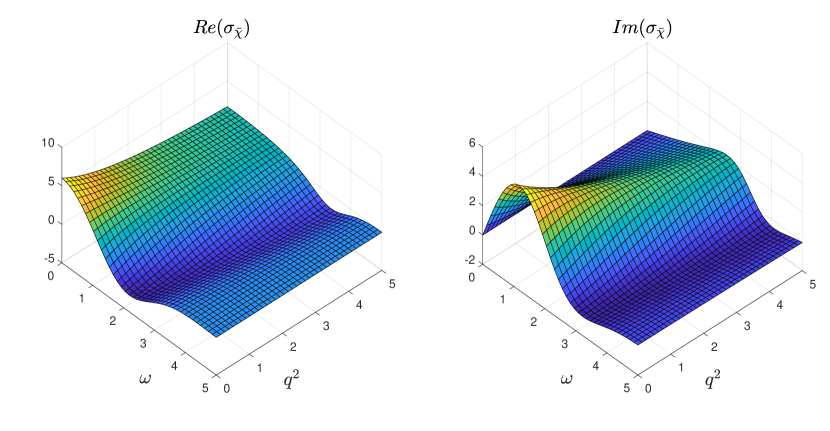
Figure 2: The generalised CME/CSE conductivity $\sigma_{\bar{\chi}}$ as a function of $\omega$ and $q^{2}$.

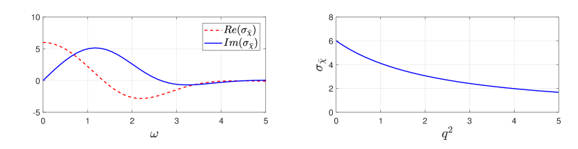
Figure 3: $\omega$-dependence of $\sigma_{\bar{\chi}}$ when $q=0$ (left); $q^{2}$-dependence of $\sigma_{\bar{\chi}}$ when $\omega=0$ (right).

Next we consider TCFs $\mathcal{D}_{H}$, $\bar{\mathcal{D}}_{H}$, $\sigma_{a\chi H}$ and $\bar{\sigma}_{a\chi H}$ multiplying second order derivative structures. These second order derivative structures are cross products between electric/magnetic fields and gradient of the densities. Via the crossing rule (IV.1), the Hall diffusion functions $\mathcal{D}_{H}$ and $\bar{\mathcal{D}}_{H}$ satisfy $\bar{\mathcal{D}}_{H}=\mathcal{D}_{H}(\bar{\mu}\leftrightarrow\bar{\mu}_{5})$. Thus, we will mainly focus on $\mathcal{D}_{H}$. $\sigma_{a\chi H}$ is the anomalous chiral Hall TCF and $\bar{\sigma}_{a\chi H}$ is its axial analogue. Since $V_{4}=q^{2}V_{5}$ and $\bar{V}_{4}=q^{2}\bar{V}_{5}$ (see (91)), from the ODE (85) it is obvious that $\bar{\sigma}_{a\chi H}$ has an overall $q^{2}$ factor, so we will plot $\bar{\sigma}_{a\chi H}/q^{2}$ in order to see non-trivial behavior.

For representative values of $\bar{\mu},\bar{\mu}_{5}$, the frequency/momentum-dependence of TCFs $\mathcal{D}_{H}$, $\sigma_{a\chi H}$ and $\bar{\sigma}_{a\chi H}$ is displayed in Figures 4, 5, 7, 8, 10 and 11. These plots show similar behaviors as Figures 2 and 3. In contrast to $\sigma_{\bar{\chi}}$, the TCFs $\mathcal{D}_{H}$, $\sigma_{a\chi H}$ and $\bar{\sigma}_{a\chi H}$ have non-trivial dependence on the chemical potentials for nonvanishing momentum values.

Figures 6, 9, 12 display 2D slices of 4, 5, 7, 8, 10 and 11 when either $\omega=0$ or $q=0$. Recall that when $q=0$, $\mathcal{D}_{H}$ does not depend on chemical potentials, as can been checked from relevant ODEs (75, 77 ,78). Similarly, from ODEs (83, 85, 86,88) it is obvious that when $q=0$, $\bar{\sigma}_{a\chi H}$ vanishes and $\sigma_{a\chi H}$ does not depend on chemical potentials. Once $q\neq 0$, TCFs $\mathcal{D}_{H}$, $\sigma_{a\chi H}$ and $\bar{\sigma}_{a\chi H}$ depend on chemical potentials non-linearly.

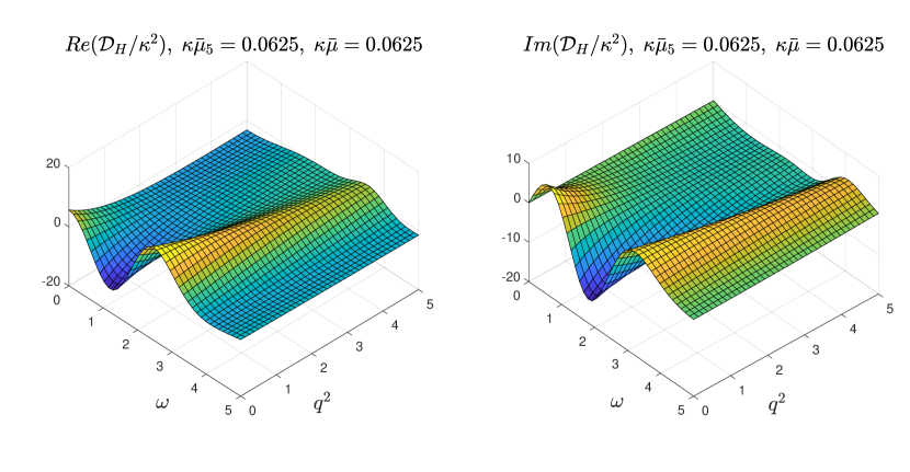
Figure 4: Hall diffusion TCF $\mathcal{D}_{H}/\kappa^{2}$ as a function of $\omega$ and $q^{2}$ when $\kappa\bar{\mu}=\kappa\bar{\mu}_{5}=1/16$.

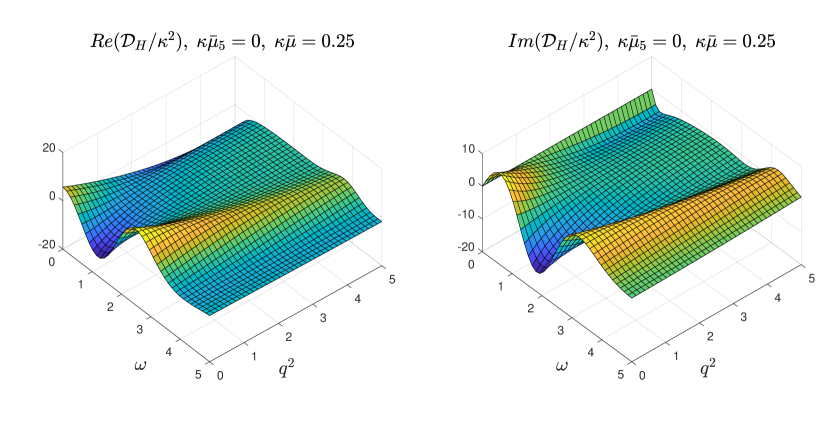
Figure 5: Hall diffusion TCF $\mathcal{D}_{H}/\kappa^{2}$ as a function of $\omega$ and $q^{2}$ when $\kappa\bar{\mu}=1/4$, $\kappa\bar{\mu}_{5}=0$.

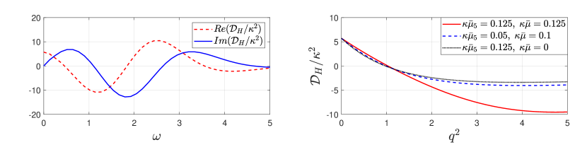
Figure 6: $\omega$-dependence of $\mathcal{D}_{H}$ when $q=0$. Here $\mathcal{D}_{H}^{0}$ stands for DC limit of $\mathcal{D}_{H}$.

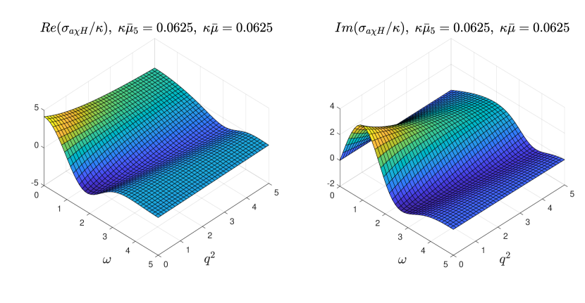
Figure 7: Anomalous chiral Hall TCF $\sigma_{a\chi H}/\kappa$ as a function of $\omega$ and $q^{2}$ when $\kappa\bar{\mu}=\kappa\bar{\mu}_{5}=1/16$.

Figure 8: Anomalous chiral Hall TCF $\sigma_{a\chi H}/\kappa$ as a function of $\omega$ and $q^{2}$ when $\kappa\bar{\mu}=\kappa\bar{\mu}_{5}=1/8$.

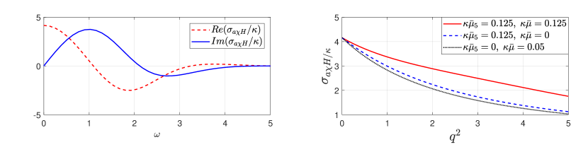
Figure 9: $\omega$-dependence of $\sigma_{a\chi H}/\kappa$ when $q=0$ (left); $q^{2}$-dependence of $\sigma_{a\chi H}$ when $\omega=0$ (right).

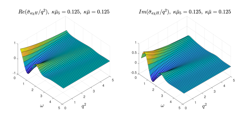
Figure 10: TCF $\bar{\sigma}_{a\chi H}/q^{2}$ as a function of $\omega$ and $q^{2}$ when $\kappa\bar{\mu}=\kappa\bar{\mu}_{5}=1/8$.

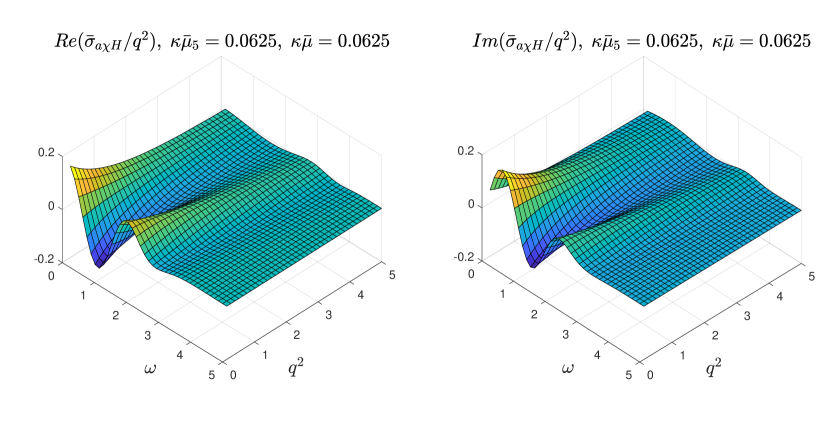
Figure 11: TCF $\bar{\sigma}_{a\chi H}/q^{2}$ as a function of $\omega$ and $q^{2}$ when $\kappa\bar{\mu}=\kappa\bar{\mu}_{5}=1/16$.

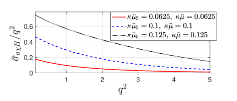
Figure 12: $q^{2}$-dependence of $\bar{\sigma}_{a\chi H}$ when $\omega=0$.

Finally, we turn to the remaining TCFs $\sigma_{1,2,3}$ and $\bar{\sigma}_{3}$ which multiply third order derivative structures. The $\sigma_{2}$ and $\bar{\sigma}_{3}$ could be thought of as the axial analogues of $\sigma_{1}$ and $\sigma_{3}$, respectively. While $\sigma_{2}$ still has nonzero value when both $\kappa\bar{\mu}$ and $\kappa\bar{\mu}_{5}$ vanish, $\sigma_{1}$ relies on that $\kappa\bar{\mu}\bar{\mu}_{5}\neq 0$. Without loss of generality, we take $\kappa\bar{\mu}\geq\kappa\bar{\mu}_{5}$ when making plots for $\sigma_{1,2}$. Note that given the crossing rule (IV.1), $\bar{\sigma}_{3}$ can be extracted from $\sigma_{3}$ by $\bar{\mu}\leftrightarrow\bar{\mu}_{5}$. For representative choices of $\bar{\mu},\bar{\mu}_{5}$, the 3D plots of these TCFs are summarised in Figures 13, 15, 16, 18 and 19. In Figures 14, 17 and 20 we depict 2D slices of Figures 13, 15, 16, 18 and 19 when either $q=0$ or $\omega=0$. As for $\mathcal{D}_{H}$, $\sigma_{a\chi H}$ and $\bar{\sigma}_{a\chi H}$, for nonzero $q$, $\sigma_{1,2,3}$ and $\bar{\sigma}_{3}$ depend on chemical potentials non-linearly.

The universal dependence on vector/axial potentials at $q=0$ is revealed by considering the normalized quantities $\sigma_{1}/\sigma_{1}^{0}$, $\sigma_{3}/\sigma_{3}^{0}$, $\delta\sigma_{2}/\delta\sigma_{2}^{0}$. Here $\sigma_{1}^{0}$, $\sigma_{3}^{0}$, $\delta\sigma_{2}^{0}$ stands for DC limit of the corresponding TCFs and $\delta\sigma_{2}=\sigma_{2}-\sigma_{2}(\kappa\bar{\mu}=\kappa\bar{\mu}_{5}=0)$. As seen from (76) and (79), $\sigma_{1}/\sigma_{1}^{0}$ and $\delta\sigma_{2}/\delta\sigma_{2}^{0}$ are identical at $q=0$. Thus, we will mainly focus on $\sigma_{1}/\sigma_{1}^{0}$. $\omega$-dependence of $\sigma_{1}/\sigma_{1}^{0}$ and $\sigma_{3}/\sigma_{3}^{0}$ is displayed in Figures 14 and 20. We observe the universal dependence of vector/axial potentials at $q=0$, that is to say these normalised quantities do not depend on chemical potentials. Explicitly, $\sigma_{1}$ is linear in $\kappa^{2}\bar{\mu}\bar{\mu}_{5}$. $\sigma_{3}$ is linear in $\kappa\bar{\mu}$. $\sigma_{2}$ has anomalous correction which is linear in $\kappa^{2}(\bar{\mu}^{2}+\bar{\mu}_{5}^{2})$. All these features can also be realised from the corresponding ODEs. Note that by employing crossing rule (IV.1), $\bar{\sigma}_{3}$ is linear in $\kappa\bar{\mu}_{5}$.

Figure 13: TCF $\sigma_{1}$ as a function of $\omega$ and $q^{2}$ when $\kappa\bar{\mu}=\kappa\bar{\mu}_{5}=1/8$.

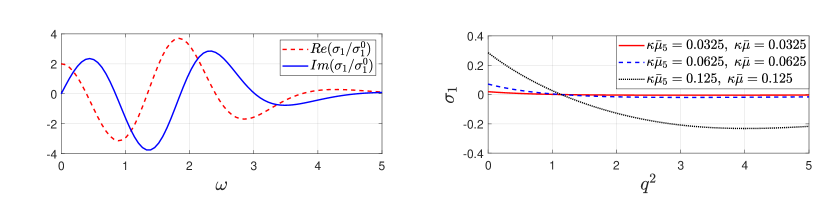
Figure 14: $\omega$-dependence of $\sigma_{1}/\sigma_{1}^{0}$ when $q=0$ (left); $q^{2}$-dependence of $\sigma_{1}$ when $\omega=0$ (right).

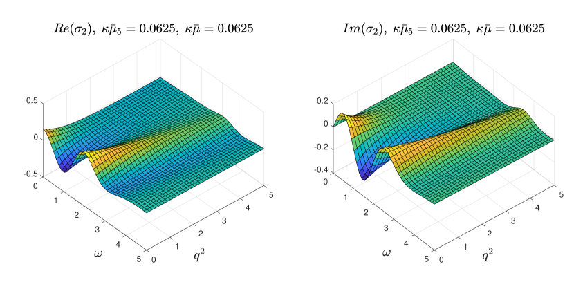
Figure 15: TCF $\sigma_{2}$ as a function of $\omega$ and $q^{2}$ when $\kappa\bar{\mu}=\kappa\bar{\mu}_{5}=1/16$.

Figure 16: TCF $\sigma_{2}$ as a function of $\omega$ and $q^{2}$ when $\kappa\bar{\mu}=1/4$, $\kappa\bar{\mu}_{5}=0$.

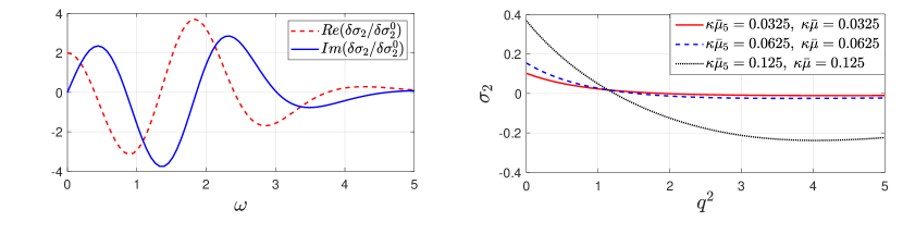
Figure 17: $\omega$-dependence of $\delta\sigma_{2}/\delta\sigma_{2}^{0}$ when $q=0$ (left); $q^{2}$-dependence of $\sigma_{2}$ when $\omega=0$ (right).

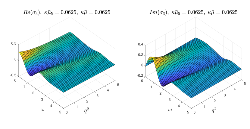
Figure 18: Conductivity $\sigma_{3}$ as a function of $\omega$ and $q^{2}$ when $\kappa\bar{\mu}=\kappa\bar{\mu}_{5}=1/16$.

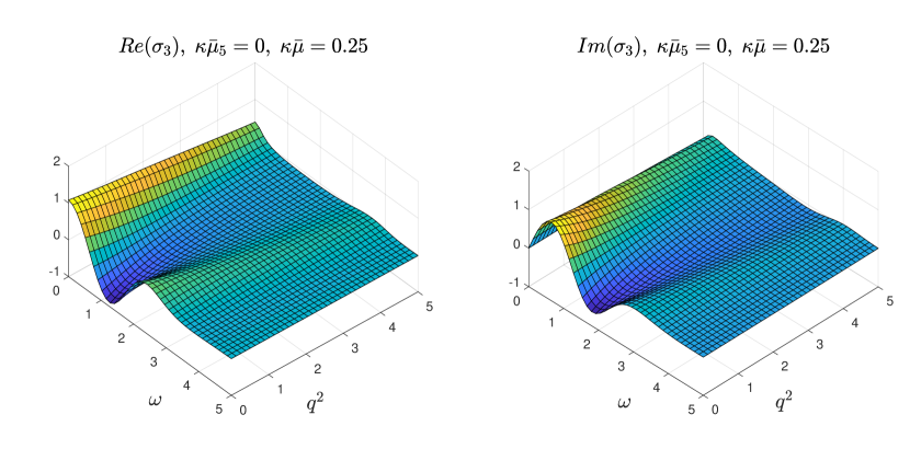
Figure 19: Conductivity $\sigma_{3}$ as a function of $\omega$ and $q^{2}$ when $\kappa\bar{\mu}=1/4$, $\kappa\bar{\mu}_{5}=0$.

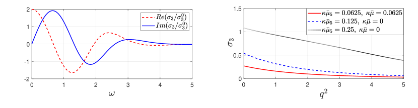
Figure 20: $\omega$-dependence of $\sigma_{3}/\sigma_{3}^{0}$ when $q=0$ (left); $q^{2}$-dependence of $\sigma_{3}$ when $\omega=0$ (right).

IV.4 CMW dispersion relation to all orders: non-dissipative modes

The TCF $\sigma_{\bar{\chi}}$ enters the dispersion relation of CMW:

$$\omega=\pm\sigma_{\bar{\chi}}(\omega,q^{2})\,\kappa\vec{q}\cdot\vec{\bf B}-i\mathcal{D}(\omega,q^{2})q^{2}.$$ (71)

The dispersion relation (71) is exact to all orders in $q^{2}$, provided $\kappa{\bf B}\ll 1$. General solutions of this equation are complex and cannot be studied with our present results. This is because $\sigma_{\bar{\chi}}(\omega,q^{2})$ and $\mathcal{D}(\omega,q^{2})$ have been computed for real values of $\omega$ only. We believe that beyond the hydrodynamic limit, equation (11) has infinitely many gapped modes. Exploring this point in general would require going into complex $\omega$ plane for the TCFs, which is beyond the scope of the present work. Yet, quite intriguingly, there is a set of purely real non-dissipative solutions to (71). In order to find these solutions we have devised the following procedure.

First, the equation is split into real and imaginary parts (assuming $\vec{q}$ parallel to $\vec{\bf B}$):

$$\phi_{I}(\omega,q^{2},\kappa{\bf B}) \equiv\rm Im[\sigma_{\bar{\chi}}(\omega,q^{2})]\,\kappa q{\bf B}-Re[\mathcal{D}(\omega,q^{2})]\,q^{2},$$

$$\phi_{R}(\omega,q^{2},\kappa{\bf B}) \equiv-\omega+\rm Re[\sigma_{\bar{\chi}}(\omega,q^{2})]\,\kappa q{\bf B}+Im[\mathcal{D}(\omega,q^{2})]\,q^{2}.$$ (72)

For a fixed value of $\kappa{\bf B}$, say $\kappa{\bf B}=0.33$, the functions $\phi_{I}$ and $\phi_{R}$ are shown in Figure 21 (left) as contour plots in $(\omega,q^{2})$ space (the function $\mathcal{D}(\omega,q^{2})$ is taken from 1511.08789 ). The dashed (blue) and solid (red) curves stand for $\phi_{I}$ and $\phi_{R}$ respectively. The numbers indicated on the curves correspond to the values of these functions along the curves. Our interest is when both functions vanish simultaneously, that is a crossing point of $\phi_{I}=0$ and $\phi_{R}=0$ curves. Such crossing is clearly seen in the region $\omega<0.5$ and $q^{2}<0.5$. We denote this point by ($\omega_{B},q_{B}$). This is a discrete density wave mode propagating in the medium without any dissipation.

The procedure could be repeated for other values of $\kappa{\bf B}$. The result is a one dimensional curve in a 3d parameter space depicted in Fig. 21 (right). A few comments are in order. First, there is a minimal value of $\kappa{\bf B}\simeq 0.33$ for which there exists such a solution. Second, in fact there are multiple solutions corresponding to several disconnected branches in Figure 21, which we do not display.

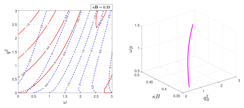
Figure 21: Contour plots for the functions $\phi_{R}$ (blue dashed) and $\phi_{I}$ (red solid) at $\kappa{\bf B}=0.33$ (left); continuum of discrete non-dissipative modes ($\omega_{B},q_{B}$) as function of $\kappa{\bf B}$ (right).

V Conclusion

In this work, we have continued exploration of nonlinear chiral anomaly-induced transport phenomena based on a holographic model with two $U(1)$ fields interacting via gauge Chern-Simons terms. For a finite temperature system, we constructed off-shell constitutive relations for the vector and axial currents.

The constitutive relations contain nine terms which are linear simultaneously in the charge density fluctuations and constant background external fields. The nine terms summarised in (7,8) correspond to all order resummation of gradients of the the charge density fluctuations parameterised by TCFs, first computed analytically in the hydrodynamic limit (section IV.2) and then numerically for large frequency/momentum (section IV.3). A common feature of all TCFs in (7,8) is that they depend weakly on spatial momentum but display pronounced dependence on frequency in the form of damped oscillations vanishing asymptotically at $\omega\simeq 5$.

Most of our results are presented in Summary section III. Among new results worth highlighting is the CME memory function computation $\tilde{\sigma}_{\bar{\chi}}(t-t^{\prime})$. The memory function is found to differ dramatically from a delta-function form of instantaneous response. In fact, $\tilde{\sigma}_{\bar{\chi}}(t-t^{\prime})$ vanishes at $t=t^{\prime}$ and the CME response gets built only after a finite amount of time of order temperature.

Another result we find of interest is related to CMW dispersion relation, which for the first time was considered to all orders in momentum $q$. Beyond the perturbative hydrodynamic limit, we found a continuum set of discrete density wave modes, which can propagate in the medium without any dissipation. While the original CMW dissipates and that could be one of the problems for its detection, the new modes that we discover should be long lived and have some potential experimental signature. It is important to remember that our calculation of the CMW dispersion relation is done for a weak magnetic field only. One can obviously question the validity of the results beyond this approximation. Both TCFs $\sigma_{\bar{\chi}}$ and $\mathcal{D}$ that enter the CMW dispersion relation are functions of $\vec{\bf E}$ and $\vec{\bf B}$. In our previous work Bu:2018psl , we initiated this study, still in perturbative in $\vec{\bf E}$ and $\vec{\bf B}$ regions, but a full non-perturbative analysis will be reported elsewhere Part3 .

We have found a wealth of non-linear phenomena all induced entirely by the chiral anomaly. An important next step in deriving a full chiral MHD would be to abandon the probe limit adopted in this paper and include the dynamics of a neutral flow as well. This will bring into the picture additional effects such as thermoelectric conductivities, normal Hall current, the chiral vortical effect 0809.2488 ; 0809.2596 , and some nonlinear effects discussed in 1603.03620 . We plan to address these in the future.

Appendix A Supplement for section IV

A.1 ODEs and the constraints for the decomposition coefficients in (49-52)

We first collect the ODEs satisfied by the decomposition coefficients in (49-52) and then derive some constraint relations obeyed by these coefficients. Plugging (49-52) into (45-48) and performing Fourier transform $\partial_{\mu}\rightarrow(-i\omega,i\vec{q})$, we obtained ODEs for the decomposition coefficients $S_{i},\bar{S}_{i},V_{i},\bar{V}_{i}$. These ODEs can be grouped into partially decoupled sub-sectors:
sub-sector (i): $\{S_{1},\bar{S}_{1},V_{1},\bar{V_{1}},V_{2},\bar{V_{2}},V_{3},\bar{V_{3}}\}$

$$0=r^{2}\partial_{r}^{2}S_{1}+3r\partial_{r}S_{1}+\partial_{r}(V_{1}-q^{2}V_{2}),$$ (73)

$$0=r^{2}\partial_{r}^{2}\bar{S}_{1}+3r\partial_{r}\bar{S}_{1}+\partial_{r}(\bar{V}_{1}-q^{2}\bar{V}_{2})+\frac{12}{r}\partial_{r}g_{4},$$ (74)

$$0=(r^{5}-r)\partial_{r}^{2}V_{1}+(3r^{4}+1-2i\omega r^{3})\partial_{r}V_{1}-(i\omega r^{2}+q^{2}r)V_{1}-\frac{12q^{2}}{r}\kappa(\bar{\rho}_{5}V_{3}+\bar{\rho}\bar{V}_{3}),$$ (75)

$$\begin{split}0&=(r^{5}-r)\partial_{r}^{2}V_{2}+(3r^{4}+1-2i\omega r^{3})\partial_{r}V_{2}-i\omega r^{2}V_{2}-rV_{1}-r^{2}(S_{1}+r\partial_{r}S_{1})\\ &-\frac{12\kappa}{r}(\bar{\rho}_{5}V_{3}+\bar{\rho}\bar{V}_{3}),\end{split}$$ (76)

$$\begin{split}0&=(r^{5}-r)\partial_{r}^{2}V_{3}+(3r^{4}+1-2i\omega r^{3})\partial_{r}V_{3}-(i\omega r^{2}+q^{2}r)V_{3}-\frac{12\kappa}{r}(\bar{\rho}_{5}V_{1}+\bar{\rho}\bar{V_{1}})\\ &+12\kappa\bar{\rho}r^{2}\partial_{r}f_{2}(i\omega g_{4}+g_{3}),\end{split}$$ (77)

$$\begin{split}0&=(r^{5}-r)\partial_{r}^{2}\bar{V}_{1}+(3r^{4}+1-2i\omega r^{3})\partial_{r}\bar{V}_{1}-(i\omega r^{2}+q^{2}r)\bar{V}_{1}-\frac{12q^{2}}{r}\kappa(\bar{\rho}V_{3}+\bar{\rho}_{5}\bar{V}_{3})\\ &+\frac{12}{r}(1+r^{3}\partial_{r}g_{3}),\end{split}$$ (78)

$$\begin{split}0&=(r^{5}-r)\partial_{r}^{2}\bar{V}_{2}+(3r^{4}+1-2i\omega r^{3})\partial_{r}\bar{V}_{2}-i\omega r^{2}\bar{V}_{2}-r\bar{V}_{1}-r^{2}(\bar{S}_{1}+r\partial_{r}\bar{S}_{1})\\ &-\frac{12\kappa}{r}(\bar{\rho}V_{3}+\bar{\rho}_{5}\bar{V}_{3}),\end{split}$$ (79)

$$\begin{split}0&=(r^{5}-r)\partial_{r}^{2}\bar{V}_{3}+(3r^{4}+1-2i\omega r^{3})\partial_{r}\bar{V}_{3}-(i\omega r^{2}+q^{2}r)\bar{V}_{3}-\frac{12\kappa}{r}(\bar{\rho}V_{1}+\bar{\rho}_{5}\bar{V_{1}})\\ &+12\kappa\bar{\rho}_{5}r^{2}\partial_{r}f_{2}(i\omega g_{4}+g_{3})-6\kappa\bar{\rho}_{5}\partial_{r}f_{2}.\end{split}$$ (80)

sub-sector (ii): $\{S_{2},\bar{S}_{2},V_{4},\bar{V_{4}},V_{5},\bar{V_{5}},V_{6},\bar{V_{6}}\}$

$$0=r^{2}\partial_{r}^{2}S_{2}+3r\partial_{r}S_{2}+\partial_{r}(V_{4}-q^{2}V_{5}),$$ (81)

$$0=r^{2}\partial_{r}^{2}\bar{S}_{2}+3r\partial_{r}\bar{S}_{2}+\partial_{r}(\bar{V}_{4}-q^{2}\bar{V}_{5}),$$ (82)

$$0=(r^{5}-r)\partial_{r}^{2}V_{4}+(3r^{4}+1-2i\omega r^{3})\partial_{r}V_{4}-(i\omega r^{2}+q^{2}r)V_{4}-\frac{12q^{2}}{r}\kappa(\bar{\rho}_{5}V_{6}+\bar{\rho}\bar{V}_{6}),$$ (83)

$$\begin{split}0&=(r^{5}-r)\partial_{r}^{2}V_{5}+(3r^{4}+1-2i\omega r^{3})\partial_{r}V_{5}-i\omega r^{2}V_{5}-rV_{4}-r^{2}(S_{2}+r\partial_{r}S_{2})\\ &-\frac{12\kappa}{r}(\bar{\rho}_{5}V_{6}+\bar{\rho}\bar{V}_{6}),\end{split}$$ (84)

$$0=(r^{5}-r)\partial_{r}^{2}V_{6}+(3r^{4}+1-2i\omega r^{3})\partial_{r}V_{6}-(i\omega r^{2}+q^{2}r)V_{6}-\frac{12\kappa}{r}(\bar{\rho}_{5}V_{4}+\bar{\rho}\bar{V_{4}}),$$ (85)

$$0=(r^{5}-r)\partial_{r}^{2}\bar{V}_{4}+(3r^{4}+1-2i\omega r^{3})\partial_{r}\bar{V}_{4}-(i\omega r^{2}+q^{2}r)\bar{V}_{4}-\frac{12q^{2}}{r}\kappa(\bar{\rho}V_{6}+\bar{\rho}_{5}\bar{V}_{6}),$$ (86)

$$\begin{split}0&=(r^{5}-r)\partial_{r}^{2}\bar{V}_{5}+(3r^{4}+1-2i\omega r^{3})\partial_{r}\bar{V}_{5}-i\omega r^{2}\bar{V}_{5}-r\bar{V}_{4}-r^{2}(\bar{S}_{2}+r\partial_{r}\bar{S}_{2})\\ &-\frac{12\kappa}{r}(\bar{\rho}V_{6}+\bar{\rho}_{5}\bar{V}_{6}),\end{split}$$ (87)

$$\begin{split}0&=(r^{5}-r)\partial_{r}^{2}\bar{V}_{6}+(3r^{4}+1-2i\omega r^{3})\partial_{r}\bar{V}_{6}-(i\omega r^{2}+q^{2}r)\bar{V}_{6}-\frac{12\kappa}{r}(\bar{\rho}V_{4}+\bar{\rho}_{5}\bar{V}_{4})\\ &-12r^{2}\left[\partial_{r}g_{4}-\partial_{r}f_{1}(i\omega g_{4}+g_{3})\right]-6\partial_{r}f_{1}.\end{split}$$ (88)

The remaining decomposition coefficients satisfy the same ODEs as above. More specifically, the sub-sector $\{\bar{S}_{3},S_{3},\bar{V}_{7},V_{7},\bar{V}_{8},V_{8},\bar{V}_{9},V_{9}\}$ satisfies the same equations as the sub-sector (i): $\{S_{1},\bar{S}_{1},V_{1},\bar{V_{1}},V_{2},\bar{V_{2}},V_{3},\bar{V_{3}}\}$; the sub-sector $\{\bar{S}_{4},S_{4},\bar{V}_{10},V_{10},\bar{V_{11}},V_{11},\bar{V}_{12},V_{12}\}$ obeys the same equations as sub-sector (ii): $\{S_{2},\bar{S}_{2},V_{4},\bar{V_{4}},V_{5},\bar{V_{5}},V_{6},\bar{V_{6}}\}$.

In what follows, we explore some “mirror symmetry relations” among these decomposition coefficients, which are useful in simplifying the expressions for currents’ constitutive relations at the order $\mathcal{O}(\epsilon^{1}\alpha^{1})$. First, notice that

$$\{S_{3},\bar{S}_{3},V_{7},\bar{V_{7}},V_{8},\bar{V_{8}},V_{9},\bar{V_{9}}\}=\{\bar{S}_{1},S_{1},\bar{V}_{1},V_{1},\bar{V}_{2},V_{2},\bar{V}_{3},V_{3}\},$$ (89)

since these two sub-sectors satisfy identical system of ODEs and have the same boundary conditions. Following this reasoning,

$$\{S_{4},\bar{S}_{4},V_{10},\bar{V}_{10},V_{11},\bar{V_{11}},V_{12},\bar{V_{12}}\}=\{\bar{S}_{2},S_{2},\bar{V}_{4},V_{4},\bar{V}_{5},V_{5},\bar{V}_{6},V_{6}\}.$$ (90)

The “equal sign” in (89,90) should be understood in the specific order as shown therein.

Certain relations can be established among the decomposition coefficients in (49-52).It follows from the Landau frame convention (62) and boundary conditions (55,56) that

$$\begin{split}&S_{1}=0,\qquad V_{1}-q^{2}V_{2}=0,\qquad S_{2}=0,\qquad V_{4}-q^{2}V_{5}=0\\ &\bar{S}_{2}=0,\qquad\qquad\bar{V}_{4}-q^{2}\bar{V}_{5}=0.\end{split}$$ (91)

Now lets explore the mirror symmetry for the decomposition coefficients under exchange $\bar{\rho}\leftrightarrow\bar{\rho}_{5}$. The decomposition coefficients in the sub-sector $\{S_{1},\bar{S}_{1},V_{1},\bar{V_{1}},V_{2},\bar{V_{2}},V_{3},\bar{V_{3}}\}$ are found symmetric with respect to $\bar{\rho},\bar{\rho}_{5}$:

$$\begin{split}&V_{i}(\bar{\rho},\bar{\rho}_{5})=V_{i}(\bar{\rho}_{5},\bar{\rho}),\qquad\bar{V}_{i}(\bar{\rho},\bar{\rho}_{5})=\bar{V}_{i}(\bar{\rho}_{5},\bar{\rho}),\qquad i=1,2,3,\\ &S_{1}(\bar{\rho},\bar{\rho}_{5})=S_{1}(\bar{\rho}_{5},\bar{\rho}),\qquad\bar{S}_{1}(\bar{\rho},\bar{\rho}_{5})=\bar{S}_{1}(\bar{\rho}_{5},\bar{\rho}).\end{split}$$ (92)

Similarly, in the second sub-sector $\{S_{2},\bar{S}_{2},V_{4},\bar{V_{4}},V_{5},\bar{V_{5}},V_{6},\bar{V_{6}}\}$,

$$\begin{split}&\bar{S}_{2}(\bar{\rho},\bar{\rho}_{5})=S_{2}(\bar{\rho}_{5},\bar{\rho}),\qquad\bar{V}_{i}(\bar{\rho},\bar{\rho}_{5})=V_{i}(\bar{\rho}_{5},\bar{\rho}),\qquad i=4,5\\ &V_{6}(\bar{\rho},\bar{\rho}_{5})=V_{6}(\bar{\rho}_{5},\bar{\rho}),\qquad\bar{V}_{6}(\bar{\rho},\bar{\rho}_{5})=\bar{V}_{6}(\bar{\rho}_{5},\bar{\rho}).\end{split}$$ (93)

The symmetry relations (92,93) guide the choice of values for $\kappa\bar{\rho}$ and $\kappa\bar{\rho}_{5}$ in numerical procedure for the ODEs. Given these relations, the choice $\kappa\bar{\rho}\geqslant\kappa\bar{\rho}_{5}$ can be applied when solving $\left\{V_{1},\bar{V}_{1},V_{3},\bar{V}_{3}\right\}$, $\left\{S_{1},V_{2},\bar{S}_{1},\bar{V}_{2}\right\}$ and $\left\{V_{4},\bar{V}_{4},V_{6},\bar{V}_{6}\right\}$ without loosing generality. These relations also help to reduce the number of the ODEs to be solved.

A.2 Perturbative solutions

Here, we summarise the perturbative solutions of (73-88) in the hydrodynamic limit $\omega,q\ll 1$. Recall that the decomposition coefficients are formally expanded as (70). Then, at each order in the hydrodynamic expansion, solutions are expressed as double integrals over $r$. The final results, up to third order in derivative expansion, are listed below.
sub-sector (i): $\left\{S_{1},\bar{S}_{1},V_{1},\bar{V}_{1},V_{2},\bar{V}_{2},V_{3},\bar{V}_{3}\right\}$:

$$S_{1}^{(0)}=V_{1}^{(0)}=0,$$ (94)

$$\bar{V}_{1}^{(0)}=\int^{\infty}_{r}\frac{xdx}{x^{4}-1}\int^{x}_{1}dy\frac{12}{y^{3}}=3\log\frac{1+r^{2}}{r^{2}}\xrightarrow[]{r\rightarrow\infty}\frac{3}{r^{2}}+\mathcal{O}\left(\frac{1}{r^{3}}\right),$$ (95)

$$\bar{S}_{1}^{(0)}=-\int^{\infty}_{r}\frac{dx}{x^{3}}\int^{\infty}_{x}dy\left[y\partial_{y}\bar{V}_{1}^{(0)}+12\partial_{y}g_{4}^{(0)}\right]\xrightarrow[]{r\rightarrow\infty}\mathcal{O}\left(\frac{1}{r^{3}}\right),$$ (96)

$$V_{3}^{(0)}=-\int^{\infty}_{r}\frac{xdx}{x^{4}-1}\int^{x}_{1}dy\frac{6\kappa}{y^{3}}\bar{\rho}\left[2\bar{V}_{1}^{(0)}+y\partial_{y}f_{2}\right]\xrightarrow[]{r\rightarrow\infty}\frac{9\kappa\bar{\rho}}{r^{2}}(2-3\log 2)+\mathcal{O}\left(\frac{1}{r^{3}}\right),$$ (97)

$$\bar{V}_{3}^{(0)}=-\int^{\infty}_{r}\frac{xdx}{x^{4}-1}\int^{x}_{1}dy\frac{6\kappa}{y^{3}}\bar{\rho}_{5}\left[2\bar{V}_{1}^{(0)}+y\partial_{y}f_{2}\right]\xrightarrow[]{r\rightarrow\infty}\frac{9\kappa\bar{\rho}_{5}}{r^{2}}(2-3\log 2)+\mathcal{O}\left(\frac{1}{r^{3}}\right),$$ (98)

$$\begin{split}V_{2}^{(0)}&=-\int^{\infty}_{r}\frac{xdx}{x^{4}-1}\int^{x}_{1}dy\frac{12\kappa}{y^{3}}(\bar{\rho}_{5}V_{3}^{(0)}+\bar{\rho}\bar{V}_{3}^{(0)})\\ &\xrightarrow[]{r\rightarrow\infty}\frac{27\kappa^{2}\bar{\rho}\bar{\rho}_{5}}{r^{2}}[6+\log 2(5\log 2-12)]+\mathcal{O}\left(\frac{1}{r^{3}}\right),\end{split}$$ (99)

$$\bar{V}_{2}^{(0)}=-\int^{\infty}_{r}\frac{xdx}{x^{4}-1}\int^{x}_{1}dy\left[\bar{S}_{1}^{(0)}+y\partial_{y}\bar{S}_{1}^{(0)}+\frac{1}{y}\bar{V}_{1}^{(0)}+\frac{12\kappa}{y^{3}}(\bar{\rho}V_{3}^{(0)}+\bar{\rho}_{5}\bar{V}_{3}^{(0)})\right]$$ (100)

$$\qquad\quad\xrightarrow[]{r\rightarrow\infty}\frac{1}{2r^{2}}\left\{\frac{1}{8}(6\pi-\pi^{2}-12\log 2)+27\kappa^{2}(\bar{\rho}^{2}+\bar{\rho}_{5}^{2})[6+\log 2(5\log 2-12)]\right\}+\mathcal{O}\left(\frac{1}{r^{3}}\right),$$

$$S_{1}^{(1)}=V_{1}^{(1)}=0,$$ (101)

$$\bar{V}_{1}^{(1)}=\int^{\infty}_{r}\frac{xdx}{x^{4}-1}\int^{x}_{1}dy\left[i\omega\bar{V}_{1}^{(0)}+2i\omega y\partial_{y}\bar{V}_{1}^{(0)}\right]\xrightarrow[]{r\rightarrow\infty}\frac{3i\omega}{4r^{2}}(\pi+2\log 2)+\mathcal{O}\left(\frac{1}{r^{3}}\right),$$ (102)

$$\bar{S}_{1}^{(1)}=-\int^{\infty}_{r}\frac{dx}{x^{3}}\int^{\infty}_{x}dy\left[y\partial_{y}\bar{V}_{1}^{(1)}+12\partial_{y}g_{4}^{(1)}\right]\xrightarrow[]{r\rightarrow\infty}\mathcal{O}\left(\frac{1}{r^{3}}\right),$$ (103)

$$\begin{split}V_{3}^{(1)}&=-\int^{\infty}_{r}\frac{xdx}{x^{4}-1}\int^{x}_{1}dy\left[i\omega V_{3}^{(0)}+2i\omega y\partial_{y}V_{3}^{(0)}+\frac{12\kappa}{y^{3}}\bar{\rho}\bar{V}_{1}^{(1)}-12i\omega\kappa\bar{\rho}g_{4}^{(0)}\partial_{y}f_{2}\right]\\ &\xrightarrow[]{r\rightarrow\infty}\frac{3i\omega\kappa\bar{\rho}}{4r^{2}}\left[\pi(6-2\pi-3\log 2)+\log 2(12-9\log 2)\right]+\mathcal{O}\left(\frac{1}{r^{3}}\right),\end{split}$$ (104)

$$\begin{split}\bar{V}_{3}^{(1)}&=-\int^{\infty}_{r}\frac{xdx}{x^{4}-1}\int^{x}_{1}dy\left[i\omega\bar{V}_{3}^{(0)}+2i\omega y\partial_{y}\bar{V}_{3}^{(0)}+\frac{12\kappa}{y^{3}}\bar{\rho}_{5}\bar{V}_{1}^{(1)}-12i\omega\kappa\bar{\rho}_{5}g_{4}^{(0)}\partial_{y}f_{2}\right]\\ &\xrightarrow[]{r\rightarrow\infty}\frac{3i\omega\kappa\bar{\rho}_{5}}{4r^{2}}\left[\pi(6-2\pi-3\log 2)+\log 2(12-9\log 2)\right]+\mathcal{O}\left(\frac{1}{r^{3}}\right),\end{split}$$ (105)

$$\begin{split}V_{1}^{(2)}&=-\int^{\infty}_{r}\frac{xdx}{x^{4}-1}\int^{x}_{1}dy\frac{12\kappa}{y^{3}}q^{2}(\bar{\rho}_{5}V_{3}^{(0)}+\bar{\rho}\bar{V}_{3}^{(0)})\\ &\xrightarrow[]{r\rightarrow\infty}\frac{27q^{2}\kappa^{2}\bar{\rho}\bar{\rho}_{5}}{r^{2}}[6+\log 2(5\log 2-12)]+\mathcal{O}\left(\frac{1}{r^{3}}\right),\end{split}$$ (106)

$$\begin{split}\bar{V}_{1}^{(2)}&=-\int^{\infty}_{r}\frac{xdx}{x^{4}-1}\int^{x}_{1}dy\left[2i\omega y\partial_{y}\bar{V}_{1}^{(1)}+i\omega\bar{V}_{1}^{(1)}+\frac{q^{2}}{y}\bar{V}_{1}^{(0)}+\frac{12\kappa}{y^{3}}q^{2}(\bar{\rho}V_{3}^{(0)}+\bar{\rho}_{5}\bar{V}_{3}^{(0)})-12\partial_{y}g_{3}^{(2)}\right]\\ &\xrightarrow[]{r\rightarrow\infty}-\frac{1}{16r^{2}}\left\{\omega^{2}\left[\pi^{2}+6(4\mathcal{C}+(\log 2)^{2})\right]\right.\\ &\qquad\quad\left.+q^{2}\left[6\pi+\pi^{2}-12\log 2-216\kappa^{2}(\bar{\rho}^{2}+\bar{\rho}_{5}^{2})(6+\log 2[5\log 2-12])\right]\right\}+\mathcal{O}\left(\frac{1}{r^{3}}\right),\end{split}$$ (107)

sub-sector (ii): $\left\{S_{2},\bar{S}_{2},V_{4},\bar{V}_{4},V_{5},\bar{V}_{5},V_{6},\bar{V}_{6}\right\}$:

$$S_{2}^{(0)}=\bar{S}_{2}^{(0)}=V_{4}^{(0)}=\bar{V}_{4}^{(0)}=V_{6}^{(0)}=0,$$ (108)

$$\bar{V}_{6}^{(0)}=-\int^{\infty}_{r}\frac{xdx}{x^{4}-1}\int^{x}_{1}dy6\left[2\partial_{y}g_{4}^{(0)}+\frac{1}{y^{2}}\partial_{y}f_{1}\right]\xrightarrow[]{r\rightarrow\infty}-\frac{3\log 2}{2r^{2}}+\mathcal{O}\left(\frac{1}{r^{3}}\right),$$ (109)

$$V_{5}^{(0)}=-\int^{\infty}_{r}\frac{xdx}{x^{4}-1}\int^{x}_{1}dy\frac{12\kappa}{y^{3}}\bar{\rho}\bar{V}_{6}^{(0)}\xrightarrow[]{r\rightarrow\infty}\frac{9\kappa\bar{\rho}(\log 2)^{2}}{4r^{2}}+\mathcal{O}\left(\frac{1}{r^{3}}\right),$$ (110)

$$\bar{V}_{5}^{(0)}=-\int^{\infty}_{r}\frac{xdx}{x^{4}-1}\int^{x}_{1}dy\frac{12\kappa}{y^{3}}\bar{\rho}_{5}\bar{V}_{6}^{(0)}\xrightarrow[]{r\rightarrow\infty}\frac{9\kappa\bar{\rho}_{5}(\log 2)^{2}}{4r^{2}}+\mathcal{O}\left(\frac{1}{r^{3}}\right),$$ (111)

$$S_{2}^{(1)}=\bar{S}_{2}^{(1)}=V_{4}^{(1)}=\bar{V}_{4}^{(1)}=V_{6}^{(1)}=0,$$ (112)

$$\begin{split}\bar{V}_{6}^{(1)}&=-\int^{\infty}_{r}\frac{xdx}{x^{4}-1}\int^{x}_{1}dy6\left[i\omega\bar{V}_{6}^{(0)}+2i\omega y\partial_{y}\bar{V}_{6}^{(0)}+12\partial_{y}g_{4}^{(1)}-12i\omega g_{4}^{(0)}\partial_{y}f_{1}\right]\\ &\xrightarrow[]{r\rightarrow\infty}-\frac{i\omega}{64r^{2}}(48\mathcal{C}+5\pi^{2})+\mathcal{O}\left(\frac{1}{r^{3}}\right),\end{split}$$ (113)

$$V_{4}^{(2)}=-\int^{\infty}_{r}\frac{xdx}{x^{4}-1}\int^{x}_{1}dy\frac{12\kappa}{y^{3}}q^{2}\bar{\rho}\bar{V}_{6}^{(0)}\xrightarrow[]{r\rightarrow\infty}\frac{9q^{2}\kappa\bar{\rho}(\log 2)^{2}}{4r^{2}}+\mathcal{O}\left(\frac{1}{r^{3}}\right),$$ (114)

$$\bar{V}_{4}^{(2)}=-\int^{\infty}_{r}\frac{xdx}{x^{4}-1}\int^{x}_{1}dy\frac{12\kappa}{y^{3}}q^{2}\bar{\rho}_{5}\bar{V}_{6}^{(0)}\xrightarrow[]{r\rightarrow\infty}\frac{9q^{2}\kappa\bar{\rho}_{5}(\log 2)^{2}}{4r^{2}}+\mathcal{O}\left(\frac{1}{r^{3}}\right),$$ (115)

where $\mathcal{C}$ is the Catalan constant. It is straightforward to read off the boundary data $v_{i}$ and $\bar{v}_{i}$ from the solutions presented above.

References

- (1) Y. Bu, M. Lublinsky, and A. Sharon, “Anomalous transport from holography: Part I,” JHEP 11 (2016) 093, arXiv:1608.08595 [hep-th].
- (2) Y. Bu, M. Lublinsky, and A. Sharon, “Anomalous transport from holography: Part II,” Eur. Phys. J. C77 no. 3, (2017) 194, arXiv:1609.09054 [hep-th].
- (3) M. Lublinsky and E. Shuryak, “How much entropy is produced in strongly coupled Quark-Gluon Plasma (sQGP) by dissipative effects?,” Phys. Rev. C76 (2007) 021901, arXiv:0704.1647 [hep-ph].
- (4) M. Lublinsky and E. Shuryak, “Improved Hydrodynamics from the AdS/CFT,” Phys. Rev. D80 (2009) 065026, arXiv:0905.4069 [hep-ph].
- (5) Y. Bu and M. Lublinsky, “All order linearized hydrodynamics from fluid-gravity correspondence,” Phys. Rev. D90 no. 8, (2014) 086003, arXiv:1406.7222 [hep-th].
- (6) Y. Bu and M. Lublinsky, “Linearized fluid/gravity correspondence: from shear viscosity to all order hydrodynamics,” JHEP 11 (2014) 064, arXiv:1409.3095 [hep-th].
- (7) Y. Bu and M. Lublinsky, “Linearly resummed hydrodynamics in a weakly curved spacetime,” JHEP 04 (2015) 136, arXiv:1502.08044 [hep-th].
- (8) Y. Bu, M. Lublinsky, and A. Sharon, “Hydrodynamics dual to Einstein-Gauss-Bonnet gravity: all-order gradient resummation,” JHEP 06 (2015) 162, arXiv:1504.01370 [hep-th].
- (9) I. Müller, “Zum paradoxon der wärmeleitungstheorie,” Zeitschrift für Physik 198 no. 4, (1967) 329–344.
- (10) W. Israel, “Nonstationary irreversible thermodynamics: A causal relativistic theory,” Annals of Physics 100 no. 1, (1976) 310 – 331.
- (11) W. Israel and J. Stewart, “Thermodynamics of nonstationary and transient effects in a relativistic gas,” Physics Letters A 58 no. 4, (1976) 213 – 215.
- (12) W. Israel and J. Stewart, “Transient relativistic thermodynamics and kinetic theory,” Annals of Physics 118 no. 2, (1979) 341 – 372.
- (13) Y. Bu, M. Lublinsky, and A. Sharon, “ current from the AdS/CFT: diffusion, conductivity and causality,” JHEP 04 (2016) 136, arXiv:1511.08789 [hep-th].
- (14) V. A. Kuzmin, V. A. Rubakov, and M. E. Shaposhnikov, “On the Anomalous Electroweak Baryon Number Nonconservation in the Early Universe,” Phys. Lett. 155B (1985) 36.
- (15) A. Vilenkin and D. A. Leahy, “Parity non-conservation and the origin of cosmic magnetic fields,” Astrophys. J. 254 (1982) 77–81.
- (16) V. A. Rubakov and M. E. Shaposhnikov, “Electroweak baryon number nonconservation in the early universe and in high-energy collisions,” Usp. Fiz. Nauk 166 (1996) 493–537, arXiv:hep-ph/9603208 [hep-ph]. [Phys. Usp.39,461(1996)].
- (17) D. Grasso and H. R. Rubinstein, “Magnetic fields in the early universe,” Phys. Rept. 348 (2001) 163–266, arXiv:astro-ph/0009061 [astro-ph].
- (18) M. Giovannini, “The magnetized universe,” International Journal of Modern Physics D 13 no. 03, (2004) 391–502.
- (19) D. E. Kharzeev, “Topology, magnetic field, and strongly interacting matter,” Annual Review of Nuclear and Particle Science 65 no. 1, (2015) 193–214.
- (20) D. E. Kharzeev, “The Chiral Magnetic Effect and Anomaly-Induced Transport,” Prog. Part. Nucl. Phys. 75 (2014) 133–151, arXiv:1312.3348 [hep-ph].
- (21) X.-G. Huang, “Electromagnetic fields and anomalous transports in heavy-ion collisions — A pedagogical review,” Rept. Prog. Phys. 79 no. 7, (2016) 076302, arXiv:1509.04073 [nucl-th].
- (22) ALICE Collaboration, J. Adam et al., “Charge-dependent flow and the search for the chiral magnetic wave in Pb-Pb collisions at 2.76 TeV,” Phys. Rev. C93 no. 4, (2016) 044903, arXiv:1512.05739 [nucl-ex].
- (23) CMS Collaboration, V. Khachatryan et al., “Observation of charge-dependent azimuthal correlations in -Pb collisions and its implication for the search for the chiral magnetic effect,” Phys. Rev. Lett. 118 no. 12, (2017) 122301, arXiv:1610.00263 [nucl-ex].
- (24) CMS Collaboration, A. M. Sirunyan et al., “Constraints on the chiral magnetic effect using charge-dependent azimuthal correlations in pPb and PbPb collisions at the LHC,” arXiv:1708.01602 [nucl-ex].
- (25) CMS Collaboration, A. M. Sirunyan et al., “Challenges to the chiral magnetic wave using charge-dependent azimuthal anisotropies in pPb and PbPb collisions at 5.02 TeV,” arXiv:1708.08901 [nucl-ex].
- (26) V. Koch, S. Schlichting, V. Skokov, P. Sorensen, J. Thomas, S. Voloshin, G. Wang, and H.-U. Yee, “Status of the chiral magnetic effect and collisions of isobars,” Chin. Phys. C41 no. 7, (2017) 072001, arXiv:1608.00982 [nucl-th].
- (27) Z. K. Liu et al., “Discovery of a Three-Dimensional Topological Dirac Semimetal, Na3Bi,” Science 343 (2015) 864–867.
- (28) B. Q. Lv et al., “Experimental discovery of Weyl semimetal TaAs,” Phys. Rev. X5 no. 3, (2015) 031013, arXiv:1502.04684 [cond-mat.mtrl-sci].
- (29) S. Y. Xu et al., “Discovery of a Weyl Fermion semimetal and topological Fermi arcs,” Science 349 (2015) 613–617.
- (30) O. Vafek and A. Vishwanath, “Dirac Fermions in Solids: From High-Tc Cuprates and Graphene to Topological Insulators and Weyl Semimetals,” Annual Review of Condensed Matter Physics 5 (Mar., 2014) 83–112, arXiv:1306.2272 [cond-mat.mes-hall].
- (31) Q. Li, D. E. Kharzeev, C. Zhang, Y. Huang, I. Pletikosic, A. V. Fedorov, R. D. Zhong, J. A. Schneeloch, G. D. Gu, and T. Valla, “Observation of the chiral magnetic effect in ZrTe5,” Nature Phys. 12 (2016) 550–554, arXiv:1412.6543 [cond-mat.str-el].
- (32) X. Huang, L. Zhao, Y. Long, P. Wang, D. Chen, Z. Yang, L. Hui, M. Xue, H. Weng, Z. Fang, X. Dai, and G. Chen, “Observation of the chiral anomaly induced negative magneto-resistance in 3D Weyl semi-metal TaAs,” Phys. Rev. X 5 (2015) 031023, arXiv:1503.01304 [cond-mat.mtrl-sci].
- (33) H. Li, H. He, H. Lu, H. Zhang, H. Liu, R. Ma, Z. Fan, S.-Q. Shen, and J. Wang, “Negative Magnetoresistance in Dirac Semimetal Cd3As2,” Nat. Commun. 7 (2016) 10301, arXiv:1507.06470 [cond-mat.str-el].
- (34) K. Landsteiner, E. Megias, and F. Pena-Benitez, “Anomalous Transport from Kubo Formulae,” Lect. Notes Phys. 871 (2013) 433–468, arXiv:1207.5808 [hep-th].
- (35) K. Landsteiner, Y. Liu, and Y.-W. Sun, “Negative magnetoresistivity in chiral fluids and holography,” JHEP 03 (2015) 127, arXiv:1410.6399 [hep-th].
- (36) A. Jimenez-Alba, K. Landsteiner, Y. Liu, and Y.-W. Sun, “Anomalous magnetoconductivity and relaxation times in holography,” JHEP 07 (2015) 117, arXiv:1504.06566 [hep-th].
- (37) K. Landsteiner and Y. Liu, “The holographic Weyl semi-metal,” Phys. Lett. B753 (2016) 453–457, arXiv:1505.04772 [hep-th].
- (38) A. Vilenkin, “Equilibrium parity-violating current in a magnetic field,” Phys. Rev. D 22 (Dec, 1980) 3080–3084.
- (39) K. Fukushima, D. E. Kharzeev, and H. J. Warringa, “The Chiral Magnetic Effect,” Phys. Rev. D78 (2008) 074033, arXiv:0808.3382 [hep-ph].
- (40) K. Fukushima, D. E. Kharzeev, and H. J. Warringa, “Real-time dynamics of the Chiral Magnetic Effect,” Phys. Rev. Lett. 104 (2010) 212001, arXiv:1002.2495 [hep-ph].
- (41) D. T. Son and A. R. Zhitnitsky, “Quantum anomalies in dense matter,” Phys. Rev. D70 (2004) 074018, arXiv:hep-ph/0405216 [hep-ph].
- (42) M. A. Metlitski and A. R. Zhitnitsky, “Anomalous axion interactions and topological currents in dense matter,” Phys. Rev. D72 (2005) 045011, arXiv:hep-ph/0505072 [hep-ph].
- (43) D. E. Kharzeev and H.-U. Yee, “Chiral Magnetic Wave,” Phys. Rev. D83 (2011) 085007, arXiv:1012.6026 [hep-th].
- (44) D. E. Kharzeev, J. Liao, S. A. Voloshin, and G. Wang, “Chiral magnetic and vortical effects in high-energy nuclear collisions—A status report,” Prog. Part. Nucl. Phys. 88 (2016) 1–28, arXiv:1511.04050 [hep-ph].
- (45) D. E. Kharzeev, “Topology, magnetic field, and strongly interacting matter,” Ann. Rev. Nucl. Part. Sci. 65 (2015) 193–214, arXiv:1501.01336 [hep-ph].
- (46) A. Avdoshkin, V. P. Kirilin, A. V. Sadofyev, and V. I. Zakharov, “On consistency of hydrodynamic approximation for chiral media,” Phys. Lett. B755 (2016) 1–7, arXiv:1402.3587 [hep-th].
- (47) J.-W. Chen, T. Ishii, S. Pu, and N. Yamamoto, “Nonlinear Chiral Transport Phenomena,” Phys. Rev. D93 no. 12, (2016) 125023, arXiv:1603.03620 [hep-th].
- (48) E. V. Gorbar, I. A. Shovkovy, S. Vilchinskii, I. Rudenok, A. Boyarsky, and O. Ruchayskiy, “Anomalous Maxwell equations for inhomogeneous chiral plasma,” Phys. Rev. D93 no. 10, (2016) 105028, arXiv:1603.03442 [hep-th].
- (49) O. F. Dayi and E. Kilincarslan, “Nonlinear Chiral Plasma Transport in Rotating Coordinates,” Phys. Rev. D96 no. 4, (2017) 043514, arXiv:1705.01267 [hep-th].
- (50) Y. Hidaka, S. Pu, and D.-L. Yang, “Nonlinear Responses of Chiral Fluids from Kinetic Theory,” Phys. Rev. D97 no. 1, (2018) 016004, arXiv:1710.00278 [hep-th].
- (51) D. E. Kharzeev and H.-U. Yee, “Anomalies and time reversal invariance in relativistic hydrodynamics: the second order and higher dimensional formulations,” Phys. Rev. D84 (2011) 045025, arXiv:1105.6360 [hep-th].
- (52) E. Megias and F. Pena-Benitez, “Holographic Gravitational Anomaly in First and Second Order Hydrodynamics,” JHEP 05 (2013) 115, arXiv:1304.5529 [hep-th].
- (53) S. Bhattacharyya, V. E. Hubeny, S. Minwalla, and M. Rangamani, “Nonlinear Fluid Dynamics from Gravity,” JHEP 02 (2008) 045, arXiv:0712.2456 [hep-th].
- (54) M. P. Heller, R. A. Janik, and P. Witaszczyk, “Hydrodynamic Gradient Expansion in Gauge Theory Plasmas,” Phys. Rev. Lett. 110 no. 21, (2013) 211602, arXiv:1302.0697 [hep-th].
- (55) M. P. Heller and M. Spalinski, “Hydrodynamics Beyond the Gradient Expansion: Resurgence and Resummation,” Phys. Rev. Lett. 115 no. 7, (2015) 072501, arXiv:1503.07514 [hep-th].
- (56) G. Basar and G. V. Dunne, “Hydrodynamics, resurgence, and transasymptotics,” Phys. Rev. D92 no. 12, (2015) 125011, arXiv:1509.05046 [hep-th].
- (57) W. Florkowski, M. P. Heller, and M. Spalinski, “New theories of relativistic hydrodynamics in the LHC era,” Rept. Prog. Phys. 81 no. 4, (2018) 046001, arXiv:1707.02282 [hep-ph].
- (58) Y. Bu, T. Demircik, and M. Lublinsky, “Nonlinear chiral transport from holography,” arXiv:1807.08467 [hep-th].
- (59) H.-U. Yee, “Holographic Chiral Magnetic Conductivity,” JHEP 11 (2009) 085, arXiv:0908.4189 [hep-th].
- (60) A. Gynther, K. Landsteiner, F. Pena-Benitez, and A. Rebhan, “Holographic Anomalous Conductivities and the Chiral Magnetic Effect,” JHEP 02 (2011) 110, arXiv:1005.2587 [hep-th].
- (61) D. T. Son and P. Surowka, “Hydrodynamics with Triangle Anomalies,” Phys. Rev. Lett. 103 (2009) 191601, arXiv:0906.5044 [hep-th].
- (62) Y. Neiman and Y. Oz, “Relativistic Hydrodynamics with General Anomalous Charges,” JHEP 03 (2011) 023, arXiv:1011.5107 [hep-th].
- (63) S. Lin, “On the anomalous superfluid hydrodynamics,” Nucl. Phys. A873 (2012) 28–46, arXiv:1104.5245 [hep-ph].
- (64) J. Bhattacharya, S. Bhattacharyya, and M. Rangamani, “Non-dissipative hydrodynamics: Effective actions versus entropy current,” JHEP 02 (2013) 153, arXiv:1211.1020 [hep-th].
- (65) N. Yamamoto, “Generalized Bloch theorem and chiral transport phenomena,” Phys. Rev. D92 no. 8, (2015) 085011, arXiv:1502.01547 [cond-mat.mes-hall].
- (66) G. Policastro, D. T. Son, and A. O. Starinets, “From AdS / CFT correspondence to hydrodynamics,” JHEP 09 (2002) 043, arXiv:hep-th/0205052 [hep-th].
- (67) K. Landsteiner, E. Megias, and F. Pena-Benitez, “Frequency dependence of the Chiral Vortical Effect,” Phys. Rev. D90 no. 6, (2014) 065026, arXiv:1312.1204 [hep-ph].
- (68) L. N. Trefethen, Spectral Methods in MATLAB. SIAM: Society for Industrial and Applied Mathematics, 2001.
- (69) J. P. Boyd, Chebyshev and Fourier Spectral Methods. Dover Publications, 2001.
- (70) T. A. Driscoll, N. Hale, and L. N. Trefethen, eds., Chebfun Guide. Pafnuty Publications, Oxford, 2014.
- (71) Y. Bu, T. Demircik, and M. Lublinsky, “Nonlinear chiral transport from holography: strong field limit,” in preparation (2018) .
- (72) J. Erdmenger, M. Haack, M. Kaminski, and A. Yarom, “Fluid dynamics of R-charged black holes,” JHEP 01 (2009) 055, arXiv:0809.2488 [hep-th].
- (73) N. Banerjee, J. Bhattacharya, S. Bhattacharyya, S. Dutta, R. Loganayagam, and P. Surowka, “Hydrodynamics from charged black branes,” JHEP 01 (2011) 094, arXiv:0809.2596 [hep-th].