NSPT estimate of the improvement coefficient $c_{A}$ to two loops

Abstract

By using Numerical Stochastic Perturbation Theory (NSPT), we carry out a quenched two-loop computation of the improvement coefficient $c_{A}$ associated to the isovector axial current. Within the Schrödinger Functional formalism, we compute the bare PCAC quark mass $m$ and fix $c_{A}$ by requiring discretization corrections on $m$ to be of order $\emph{O}(a^{2})$ in the lattice spacing $a$.

Introduction - After performing a set of numerical simulations of a generic field theory, corresponding results become meaningful only if extrapolated to the physical point ($\Phi$). This means that, given simulation parameters like — among others — lattice spacing $a$, volume $V$ and, in case, quark masses $m_{q}$, the limits $a\rightarrow 0$, $V\rightarrow+\infty$ and $m_{q}\rightarrow m_{q}^{(\Phi)}$ have to be accurately and reliably computed. While these limits were thought to be hardly accessible for lattice QCD some time ago Ukawa (2002), a few decades of algorithmic developments have paved the way to controlling all the above-mentioned sources of systematic uncertainty. Nowadays, not only $N_{f}=1+1+1+1$ QCD simulations with small lattice spacings, large boxes and quark masses close to the physical point are being performed, but also challenging QED effects have started to be taken into account Borsanyi et al. (2015).

At present, the standard setup for QCD simulations features the Hybrid Monte Carlo (HMC) algorithm Duane et al. (1987), usually supplemented with other techniques — like preconditioning DeGrand et al. (1987), the Hasenbusch trick Hasenbusch (2001), multiple time-scale integration Sexton et al. (1992) and smearing Albanese et al. (1987); Hasenfratz et al. (2001); Morningstar et al. (2004); Capitani et al. (2006). In the framework of the HMC algorithm, such techniques are useful in that they allow for a larger value of the time-step in integrating the equations of motion (thus decreasing the autocorrelation among subsequent configurations), they reduce the condition number $\kappa(D)$ of the Dirac operator $D$ (speeding up the inversion of $D$ needed both within the HMC algorithm and at measure time) and they average out ultraviolet fluctuations, improving the signal-to-noise ratio (SNR).

In this scenario, a technique often employed to reduce discretization effects is the so-called improvement, usually in a form following the Symanzik programme Symanzik (1983). To understand how the latter works, it is useful to recall that the mean value $\overline{O}$ of a generic continuum observable $O$ computed on the lattice reads

$$\overline{O}(a,V,m_{q},\ldots)=\int DUD\psi D\overline{\psi}\ \!O_{Lat}\ \!e^{-S_{Lat}}\ ,$$ (1)

where $O_{Lat}$ is the lattice counterpart of $O$, $S_{Lat}$ is the lattice QCD action (given by the sum of a gauge part $S_{G}$ and a fermionic part $S_{F}$) and where the dependence of $\overline{O}$ with respect to simulation parameters has been made explicit.

According to Symanzik, close to the continuum limit, $O_{Lat}$ can be Taylor-expanded in the lattice spacing as

$$O_{Lat}=O+aO_{1}+a^{2}O_{2}+\ldots\ ,$$ (2)

where $O_{1}$, $O_{2}$, $\ldots$ have to be interpreted as contributions stemming from operator insertions in the continuum and must have symmetry properties consistent with $O$. A similar expression holds also for the gauge and the fermionic action $S_{G}$ and $S_{F}$ entering $S_{Lat}$.

Plugging said Taylor expansions with respect to $a$ into Eq.(1) results in a similar expansion for $\overline{O}$ as well. In the Symanzik improvement programme, the leading correction to $\overline{O}$ — usually linear in $a$ as in Eq.(2) — can be cancelled by adding irrelevant terms to $S_{G}$, $S_{F}$ and to $O_{Lat}$. In this way, the dependence of $\overline{O}$ with respect to $a$ is flattened and, consequently, larger values of the lattice spacing can be used to recover the continuum limit, thereby further reducing $\emph{k}(D)$ and increasing the SNR at the same time.

In general, each irrelevant term is multiplied by its own coefficient that has to be appropriately tuned: its value can be determined either non-perturbatively or within perturbation theory (PT). Obviously, among these so-called improvement coefficients, the most important ones are those improving on $S_{G}$ and $S_{F}$ since they enter in the improvement procedure of any observable. When it comes to perturbative computations, the expansions of these coefficients in the bare coupling $g_{0}$ are usually known up to very low orders only, usually at one loop.

In this paper, we investigate whether Numerical Stochastic Perturbation Theory (NSPT) Di Renzo et al. (1994, 2004) can be applied to compute the improvement coefficients in PT to orders higher than $g_{0}^{2}$. We want to clearly state that the present study essentially aims at being a proof of concept, i.e., at assessing the feasibility — or not — of a similar NSPT computation in principle. Given such exploratory character, we tackle the simplest case possible, namely the two-loop computation of the improvement coefficient $c_{A}$ associated to the isovector axial current in the quenched approximation. In spite of its seeming minor importance, a perturbative computation of $c_{A}$ to a given order $j$ allows for a determination to the same order of the much more important coefficient $c_{SW}$, i.e., the improvement coefficient multiplying the irrelevant term improving on the fermionic action $S_{F}$ Sheikholeslami et al. (1985) which will be introduced later.

Lattice setup - In this and the next section we outline our approach which is based on the Schrödinger Functional formalism Sint (1994); Luscher et al. (1992) and closely follows the strategy described in Luscher et al. (1996) and used in Luscher et al. (1996) to compute $c_{SW}$ and $c_{A}$ to one loop.

We simulate a four-dimensional lattice made up of $N_{T}\times N_{S}^{3}$ sites, each one labelled with integer coordinates $n=(n_{0},n_{1},n_{2},n_{3})$ varying in the intervals $[0,N_{T}-1]$ and $[0,N_{S}-1]$ along the time and spatial directions respectively. The lattice volume $V$ will therefore be equal to $V=L_{T}\times L_{S}^{3}$, with $L_{T}=a(N_{T}-1)$ and $L_{S}=aN_{S}$.

A generic gauge variable $U_{\mu}(n)$ — with $\mu\in\{0,1,2,3\}$ — belongs to the $SU(3)$ group and is associated to the link connecting site $n$ to site $n+\hat{\mu}$, $\hat{\mu}$ being a unit vector along direction $\mu$. Lattice group variables are related to their continuum counterparts $A_{\mu}(n)$ in the Lie algebra of $SU(3)$ through the equation $U_{\mu}(n)=exp[iA_{\mu}(n)]$. We stick to the usual convention according to which $U^{-1}_{\mu}(n)=U^{\dagger}_{\mu}(n)$.

Quark and antiquark degrees of freedom are Grassmann variables — denoted as $\psi(n)$ and $\bar{\psi}(n)$ respectively — associated to the lattice sites. For simplicity, we assume the presence of $N_{f}$ mass-degenerate flavours though, in what follows, the fermionic action $S_{F}$ and its irrelevant term will always be written by taking into account only one flavour to ease the notation: it is understood that there are actually $N_{f}$ replicae of such operators. Anyway, it is worth stressing that, while the quenched approximation implies — obviously — that fermionic degrees of freedom play no role in updating the lattice configuration and that, consequently, the results of this paper have to be considered valid for $N_{f}=0$, the setup described in the next sections is such that $N_{f}$ never enters into play at measurement time as well, as long as the mass degeneracy holds.

While boundary conditions are periodic along the three spatial directions, they are of Dirichlet type in the time direction. In other words, by labelling a generic spatial direction with $k$ from now on, for the gauge fields the following equalities hold

$$\left.U_{k}(n)\right|_{n_{0}=0}=W_{k}(\vec{n})\ ,\ \ \ \left.U_{k}(n)\right|_{n_{0}=N_{T}-1}=W_{k}^{\prime}(\vec{n})\ ,\vspace*{0.15cm}$$ (3)

with $\vec{n}=(n_{1},n_{2},n_{3})$ and where $W_{k}(\vec{n})$ can be expressed in terms of a smooth, fixed field $C_{k}(\vec{n})$ as

$$\vspace*{0.25cm}W_{k}(\vec{n})=\mathcal{P}\ \!exp\bigg{[}a\!\!\int_{0}^{1}\!\!dt\ \!C_{k}(\vec{n}+a\hat{k}-ta\hat{k})\bigg{]}\ ,\vspace*{-0.05cm}$$ (4)

being $\mathcal{P}$ the path-ordering symbol. $\!W_{k}^{\prime}(\vec{n})$ is parametrized by another field $C_{k}^{\prime}(\vec{n})$ in an analogous way.

With this setup, the lattice gauge action $S_{G}$ is given by the modified Wilson action

$$S_{G}=\frac{1}{g_{0}^{2}}\sum_{p}\omega(p)tr\{1-U(p)\}\ ,$$ (5)

where $U(p)$ is the product of the link variables around a lattice plaquette, the sum runs on all oriented plaquettes and the weights $\omega(p)$ are equal to $1$ for each plaquette, except for the spatial ones at $n_{0}=0$ and $n_{0}=N_{T}-1$ where $\omega(p)=\frac{1}{2}$. Due to the SF boundary conditions, the gauge action $S_{G}$ in Eq.(5) with said values of the weights $\omega(p)$ is $\emph{O}(a)-$improved only at tree-level in PT. A version of $S_{G}$ that is $\emph{O}(a)-$improved at any perturbative order can be obtained by adding some boundary counterterms featuring their own improvement coefficients that have to be appropriately tuned. This whole procedure would eventually amount to a redefinition of the weights $\omega(p)$ close to the boundaries. In the present work, such $S_{G}-$related counterterms will be ignored because the observable that will be introduced and studied later on — i.e., the bare PCAC quark mass — is entirely fixed by a Ward identity and this peculiar property allows to neglect said counterterms.

As for the fermionic degrees of freedom, after introducing the projectors $P_{\pm}=\frac{1}{2}(1\pm\gamma_{0})$ — $\gamma_{0}$ being a Euclidean Dirac matrix — and some fixed Grassmann fields $\rho,\ldots,\bar{\rho}^{\prime}$, their Dirichlet boundary conditions are given by

$$\left.P_{+}\psi(n)\right|_{n_{0}=0}=\rho(\vec{n})\ ,\ \ \ \ \left.P_{-}\psi(n)\right|_{n_{0}=N_{T}-1}=\rho^{\prime}(\vec{n})\ ,\vspace{0.25cm}$$ (6)

for the quark fields and by

$$\left.\bar{\psi}(n)P_{-}\right|_{n_{0}=0}=\bar{\rho}(\vec{n})\ ,\ \ \ \left.\bar{\psi}(n)P_{+}\right|_{n_{0}=N_{T}-1}=\bar{\rho}^{\prime}(\vec{n})\ ,\vspace{0.25cm}$$ (7)

for the antiquark fields. For consistency, quantities $P_{-}\rho,\ldots,\bar{\rho}^{\prime}P_{-}$ must vanish.

The unimproved fermionic action $S_{F}$ is given by

$$S_{F}=a^{4}\sum_{n}\bar{\psi}(n)(D+m_{0})\psi(n)\ ,\vspace*{0.1cm}$$ (8)

$m_{0}$ being the bare quark mass and the Wilson-Dirac operator $D$ reading

$$D=\frac{1}{2}\bigg{[}\gamma_{\mu}(\nabla_{\mu}^{*}+\nabla_{\mu})-a\nabla_{\mu}^{*}\nabla_{\mu}\bigg{]}\ ,\vspace*{0.1cm}$$ (9)

where repeated indices are summed and $\gamma_{\mu}$’s are Euclidean Dirac matrices. Covariant derivatives in Eq.(9) are defined as

$$\!\!\!\nabla_{\mu}\psi(n) = \frac{1}{a}\big{[}\lambda_{\mu}U_{\mu}(n)\psi(n+\hat{\mu})-\psi(n)\big{]}\ ,$$

$$\!\!\!\nabla_{\mu}^{*}\psi(n) = \frac{1}{a}\big{[}\psi(n)-\lambda_{\mu}^{-1}U_{\mu}^{-1}(n-\hat{\mu})\psi(n-\hat{\mu})]\ ,$$ (10)

$\lambda_{0}=1$ and $\lambda_{k}=exp(ia\theta_{k}/L_{S})$ being phase factors (with $-\pi<\theta_{k}\leq\pi$). For simplicity, all three angles $\theta_{k}$ will be set to the same unique value $\theta\neq 0$.

Strictly speaking, Eq.(8) holds in an infinite volume. However, it remains valid also in the present setup — i.e., a box of finite size with Dirichlet boundary conditions — provided some technical conventions are assumed: the interested reader can find more details in subsection $4.2$ of Luscher et al. (1996). We tacitly take such conventions for granted and carry on with Eq.(8) in combination with said lattice topology.

The leading discretization correction to $S_{F}$ is linear in $a$ and, as mentioned in the introduction, an $\emph{O}(a)-$improved fermionic action $S_{F}^{imp}$ can be obtained by adding to Eq.(8) an irrelevant term $\delta S_{V}$, i.e.,

$$S_{F}^{imp}=S_{F}+\delta S_{V}\ .\vspace{0.2cm}$$ (11)

$\delta S_{V}$ is usually referred to as clover term and its expression is given by Sheikholeslami et al. (1985)

$$\delta S_{V}=a^{5}c_{SW}\sum_{n_{0}=1}^{N_{T}-2}\sum_{n_{1},n_{2},n_{3}=0}^{N_{S}-1}\bar{\psi}(n)\frac{i}{4}\sigma_{\mu\nu}F_{\mu\nu}(n)\psi(n)\ ,\vspace{0.2cm}$$ (12)

where $\sigma_{\mu\nu}=\frac{i}{2}[\gamma_{\mu},\gamma_{\nu}]$ and

$$F_{\mu\nu}(n)=\frac{1}{8a^{2}}\big{[}Q_{\mu\nu}(n)-Q_{\nu\mu}(n)\big{]}\ ,\vspace{0.2cm}$$ (13)

with

$$\begin{split}&Q_{\mu\nu}(n)=U_{\mu}(n)U_{\nu}(n+\hat{\mu})U^{\dagger}_{\mu}(n+\hat{\nu})U^{\dagger}_{\nu}(n)+\\ &+U_{\nu}(n)U^{\dagger}_{\mu}(n-\hat{\mu}+\hat{\nu})U^{\dagger}_{\nu}(n-\hat{\mu})U_{\mu}(n-\hat{\mu})+\\ &+U^{\dagger}_{\mu}(n-\hat{\mu})U^{\dagger}_{\nu}(n-\hat{\mu}-\hat{\nu})U_{\mu}(n-\hat{\mu}-\hat{\nu})U_{\nu}(n-\hat{\nu})+\\ &+U^{\dagger}_{\nu}(n-\hat{\nu})U_{\mu}(n-\hat{\nu})U_{\nu}(n+\hat{\mu}-\hat{\nu})U^{\dagger}_{\mu}(n)\ .\end{split}\vspace{0.2cm}$$ (14)

The perturbative expansion of the $c_{SW}$ coefficient appearing in Eq.(12) is known up to one loop and it can be written as

$$c_{SW}=c_{SW}^{(0)}+c_{SW}^{(1)}g_{0}^{2}+\emph{O}(g_{0}^{4})\ ,\vspace{0.1cm}$$ (15)

where $c_{SW}^{(0)}=1$ Sheikholeslami et al. (1985) while $c_{SW}^{(1)}$ has been computed in several papers Wohlert (1987); Luscher et al. (1996); Aoki et al. (2003); Horsley et al. (2008) yielding results slightly different but in agreement within errorbars.

Analogously to the case of the gauge action $S_{G}$, it is worth stressing that, in the present lattice setup featuring SF boundary conditions, an $\emph{O}(a)-$improved version of $S_{F}$ would require not only the addition of $\delta S_{V}$ as defined in Eq.(12), but also the introduction of boundary counterterms with corresponding improvement coefficients to be accurately tuned. Anyway, exactly as it is for the gauge action, such $S_{F}-$related boundary counterterms will be entirely neglected in this work thanks to the fact that the bare PCAC quark mass studied later on is completely fixed by a Ward identity.

Before concluding this section, it is important to observe that the bare quark mass $m_{0}$ in Eq.(8) will be set to $0$ from now on and that quarks will be kept massless by subtracting the appropriate mass counterterms order by order in PT (see Panagopoulos et al. (2003) for their calculation in infinite volume to two loops).

Methodology - The improvement coefficient $c_{A}$ targeted by this study is associated to the isovector axial current $A_{\mu}^{b}(n)$

$$A_{\mu}^{b}(n)=\bar{\psi}(n)\gamma_{\mu}\gamma_{5}\frac{1}{2}\tau^{b}\psi(n)\ ,\vspace*{0.2cm}$$ (16)

$\tau^{b}$ being a Pauli matrix acting on flavour indices and $\gamma_{5}=\gamma_{0}\gamma_{1}\gamma_{2}\gamma_{3}$ as usual. An $\emph{O}(a)-$improved expression is obtained by adding an irrelevant term $\delta A_{\mu}^{b}(n)$ reading

$$\delta A_{\mu}^{b}(n)=ac_{A}\frac{1}{2}(\delta_{\mu}^{*}+\delta_{\mu})P^{b}(n)\ ,\vspace{0.2cm}$$ (17)

where $\delta_{\mu}^{*}$ and $\delta_{\mu}$ stand for the standard left and right derivative on the lattice while $P^{b}(n)$ is the isovector axial density

$$P^{b}(n)=\bar{\psi}(n)\gamma_{5}\frac{1}{2}\tau^{b}\psi(n)\ .$$ (18)

As in Eq.(15), the improvement coefficient $c_{A}$ in Eq.(17) can be expanded as

$$c_{A}=c_{A}^{(0)}+c_{A}^{(1)}g_{0}^{2}+c_{A}^{(2)}g_{0}^{4}+\ldots\ ,\vspace{0.2cm}$$ (19)

where $c_{A}^{(0)}$ is equal to $0$ Heatlie et al. (1991), $c_{A}^{(1)}$ has been determined in Luscher et al. (1996) while estimating $c_{A}^{(2)}$ is the goal of this work.

Following Luscher et al. (1996), we begin by relating $A_{\mu}^{b}(n)$ and $P^{b}(n)$ to the unrenormalized PCAC quark mass $m$ by means of the PCAC relation

$$\Big{\langle}\frac{1}{2}(\delta_{\mu}^{*}+\delta_{\mu})A_{\mu}^{b}(n)\mathcal{O}\Big{\rangle}=2m\Big{\langle}P^{b}(n)\mathcal{O}\Big{\rangle}\ ,\vspace{0.2cm}$$ (20)

with $\mathcal{O}$ the product of fields located at non-zero distance from site $n$ and from each other. Then, we set $\mathcal{O}$ to be

$$\mathcal{O}=a^{6}\sum_{n^{\prime},n^{\prime\prime}}\bar{\zeta}(n^{\prime})\gamma_{5}\frac{1}{2}\tau^{b}\zeta(n^{\prime\prime})\ ,\vspace{0.1cm}$$ (21)

with the constraint $n^{\prime}_{0}=n^{\prime\prime}_{0}=0$ and with

$$\left.\zeta(n)\right|_{n_{0}=0}=\frac{\delta}{\delta\bar{\rho}(\vec{n})},\ \ \ \ \ \left.\bar{\zeta}(n)\right|_{n_{0}=0}=-\frac{\delta}{\delta\rho(\vec{n})}\ ,\vspace{0.2cm}$$ (22)

being $\rho(\vec{n})$ and $\bar{\rho}(\vec{n})$ the fields introduced in Eqs.(6)(7).

After defining the correlators $f_{A}(n)$ and $f_{P}(n)$ as

$$\begin{split}f_{A}(n)=-a^{6}\sum_{n^{\prime},n^{\prime\prime},b}\frac{1}{3}\Big{\langle}A_{0}^{b}(n)\bar{\zeta}(n^{\prime})\gamma_{5}\frac{1}{2}\tau^{b}\zeta(n^{\prime\prime})\Big{\rangle}\ ,\\ f_{P}(n)=-a^{6}\sum_{n^{\prime},n^{\prime\prime},b}\frac{1}{3}\Big{\langle}P^{b}(n)\bar{\zeta}(n^{\prime})\gamma_{5}\frac{1}{2}\tau^{b}\zeta(n^{\prime\prime})\Big{\rangle}\ ,\end{split}\vspace{0.2cm}$$ (23)

again with the constraint $n^{\prime}_{0}=n^{\prime\prime}_{0}=0$, the unimproved bare PCAC quark mass $m$ in Eq.(20) is given by

$$m=\frac{1}{2}\Big{[}\frac{1}{2}(\delta_{0}^{*}+\delta_{0})f_{A}(n)\Big{]}/f_{P}(n)\ .\vspace{0.2cm}$$ (24)

Noting that $P^{b}(n)$ is already $\emph{O}(a)-$improved Luscher et al. (1996) and recalling Eq.(17), the $\emph{O}(a)-$improved bare PCAC quark mass $m_{imp}$ is given by

$$m_{imp}=\frac{1}{2}\Big{[}\frac{1}{2}(\delta_{0}^{*}+\delta_{0})f_{A}(n)+ac_{A}\delta_{0}^{*}\delta_{0}f_{P}(n)\Big{]}/f_{P}(n)\ ,\vspace{0.2cm}$$ (25)

provided that the irrelevant term in Eq.(12) is also added to $S_{F}$ and that both $c_{A}$ and $c_{SW}$ are correctly set.

The last observation gives us a prescription to determine the improvement coefficients. Before explaining why, it is worth recalling that, in order to study the continuum limit of a given observable to monitor $\emph{O}(a)$ effects, such an observable must necessarily be a meaningful dimensionless quantity. In this respect, the most straightforward observable that can be built in the present case is given by the product of the lattice extent $L_{S}$ times the renormalized improved PCAC quark mass $m_{R}$, where

$$m_{R}=\frac{Z_{A}}{Z_{P}}m_{imp}\ ,\vspace{0.2cm}$$ (26)

$Z_{A}$ and $Z_{P}$ being the renormalization constants of the isovector axial current and density respectively. However, it is possible to show explicitly up to 2-loop order that the multiplicative renormalization of the PCAC quark mass as well as the renormalization of the gauge coupling can eventually be omitted for our purposes, as they only introduce $\emph{O}(a^{2})$ corrections. This provided of course that the bare quark mass $m_{0}$ in Eq.(8) is adjusted to its critical value and that $c_{A}$ is properly set up to 1-loop order. In other words, if such a setup holds, $c_{A}$ can be determined up to the second loop by studying the behaviour of the product of the unrenormalized improved PCAC quark mass $m_{imp}$ times $L_{S}$.

Bearing these observations in mind, in PT the product $m_{imp}L_{S}$ can be expanded as

$$m_{imp}L_{S}=\sum_{i=0}m_{imp}^{(i)}L_{S}g_{0}^{2i}\ ,\vspace{-0.1cm}$$ (27)

where coefficients $m_{imp}^{(i)}$ will depend on the coefficients $c_{A}$ and $c_{SW}$ and on the kinematic parameters $a$, $N_{S}$, $N_{T}$, $\theta$ as well as on the time coordinate $n_{0}$ of site $n$ in Eq.(25) — there is no dependence with respect to the spatial coordinates of $n$ because of the translational invariance along the corresponding directions. $m_{imp}$ should also depend on the boundary fields $C_{k},C_{k}^{\prime},\rho,\bar{\rho},\rho^{\prime},\bar{\rho}^{\prime}$: however, fermionic boundary fields will be set to zero after derivatives in Eq.(21) are computed while fields $C_{k}(\vec{n})$ and $C_{k}^{\prime}(\vec{n})$ will be fixed to $0$ for every $\vec{n}$ (so that $W_{k}(\vec{n})=W_{k}^{\prime}(\vec{n})=1$). The last choice will be motivated later on.

Since infinite-volume mass counterterms are subtracted up to two loops and since the product $m_{imp}L_{S}$ does not carry any dimension, both $m_{imp}^{(i)}L_{S}$ — with $i=1,2$ — can be expanded in $a$ out of dimensional analysis as

$$\begin{split}m_{imp}^{(i)}L_{S}&=d_{1,N_{S}}^{\ \!\!(i)}\frac{a}{L_{S}}+d_{1,N_{T}}^{\ \!\!(i)}\frac{a}{L_{T}}+\\ &+d_{1,\theta}^{\ \!\!(i)}\frac{a\theta}{L_{S}}+d_{1,n_{0}}^{\ \!\!(i)}\frac{a}{an_{0}}+\ldots\ ,\\ &=d_{1,N_{S}}^{\ \!\!(i)}\frac{1}{N_{S}}+d_{1,N_{T}}^{\ \!\!(i)}\frac{1}{N_{T}-1}+\\ &+d_{1,\theta}^{\ \!\!(i)}\frac{\theta}{N_{S}}+d_{1,n_{0}}^{\ \!\!(i)}\frac{1}{n_{0}}+\ldots\ ,\\ &\end{split}\vspace{0.2cm}$$ (28)

where dots denote terms of higher order in $a$ and all coefficients $d_{1,\ldots}^{\ \!\!(i)}$ depend on $c_{A}$ and $c_{SW}$ — such dependence will be left implicit to ease the notation. By setting $N_{T}=2N_{S}+1$, $n_{0}=N_{S}/2$ (as in Luscher et al. (1996)) and by keeping $\theta$ fixed, the resulting mathematical setup is such that the terms on the r.h.s. of the previous formula can be collected into one as

$$m_{imp}^{(i)}L_{S}=d^{\ \!\!(i)}_{1}\frac{1}{N_{S}}+O\bigg{(}\frac{1}{N_{S}^{2}}\bigg{)}.\vspace{0.1cm}$$ (29)

By comparing Eqs.(28) and (29), it should be evident that an expansion in powers of $a$ is equivalent to an expansion in powers of $1/N_{S}$. Bearing this observation in mind and recalling that we aim at O(a)-improvement, coefficients $c_{SW}^{(i)}$ and $c_{A}^{(i)}$ in Eqs.(15) and (19) can be determined up to two loops as follows: with the setup outlined above, the product $L_{S}$ times the bare PCAC quark mass is first measured for several values of $N_{S}$, then it is fitted vs. $1/N_{S}$ and $c_{SW}$ and $c_{A}$ are finally determined by requiring the coefficient $d^{\ \!\!(i)}_{1}$ in Eq.(29) to be compatible with zero.

In this approach, there is actually one last issue to be solved: in fact, to a given loop $i$ in PT, the coefficient $d^{\ \!\!(i)}_{1}$ depends on all $c_{A}^{(j)}$ and $c_{SW}^{(j)}$ with $j\leq i$, so that their effects have to be disentangled. This can be done by choosing the boundary fields $C_{k}$ and $C_{k}^{\prime}$ appropriately. In particular, if such fields are both set to $0$ everywhere along the time boundaries as in the present setup, it can be proven Luscher et al. (1996) that, at the lowest order in PT, the dynamical gauge degrees of freedom $U$ are $1$ throughout the whole lattice and, consequently, Eqs.(13) and (14) imply that the lowest order of $F_{\mu\nu}$ in Eq.(12) will be proportional to $g_{0}$. In turn, this means that, truncating any expansion in $g_{0}$ at a given loop $i$, only $c_{A}^{(i)}$ — as well as all coefficients at loops lower than $i$ in Eqs.(15) and (19) — will be left into play. This yields to a well-defined procedure to evaluate $c_{A}^{(2)}$: in fact, in the present situation where $c_{SW}^{(i)}$ and $c_{A}^{(i)}$ have already been determined for $i\leq 1$, by setting these tree-level and one-loop coefficients to their known values as well as the fields $C_{k}$ and $C_{k}^{\prime}$ to $0$ and by truncating any perturbative expansion at the second loop in $g_{0}$, $d^{\ \!\!(2)}_{1}$ will only depend on $c_{A}^{(2)}$ and the latter coefficient can thus be fixed by fitting $m_{imp}^{(2)}L_{S}$ with respect to $1/N_{S}$.

Though it is not the goal of this study, let us recall how $c_{SW}^{(2)}$ could be evaluated. The very same setup needed to compute $c_{A}^{(2)}$ is maintained but the fields $C_{k}$ and $C_{k}^{\prime}$ have now to be set as explained in Sect. $6.2$ of Luscher et al. (1996): fixing $c_{A}^{(2)}$ to the value found as outlined in the previous paragraphs, $d^{\ \!\!(2)}_{1}$ will now depend solely on $c_{SW}^{(2)}$, so that the correct value of the latter coefficient could be determined, again by fitting $m_{imp}^{(2)}L_{S}$ vs. $1/N_{S}$. This overall procedure can obviously be iterated to the third loop (and higher), provided that the corresponding mass counterterm is subtracted.

Before concluding this section, it is worth recalling that, within the Schrödinger Functional formalism, also boundary irrelevant terms in $a$ have in principle to be introduced in order to achieve $\emph{O}(a)-$improvement, each one with its own coefficient. However, as stated in Luscher et al. (1996), these terms can be eventually dropped and remaining improvement coefficients can be determined by solely requiring the unrenormalized PCAC quark mass to be independent of the kinematic parameters, which corresponds to the strategy outlined above.

NSPT practice - In this section we describe how configurations are generated by means of Numerical Stochastic Perturbation Theory. NSPT stems from Stochastic Quantization (SQ) Parisi et al. (1980), a quantization prescription that, in turn, inspired the so-called Langevin algorithm (described in what follows) allowing for the computation of expectation values in quantum field theories. It has been used in several domains of research, one of the latest being the search for solutions to the sign problem — see Aarts et al. (2017); Di Renzo et al. (2015) and references therein.

To introduce the basics of SQ in a simple way, we start with a lattice scalar field theory with action $S[\phi]$. In SQ its degrees of freedom $\phi(n)$ are updated by numerically integrating a Langevin equation reading

$$\frac{\partial\phi(n,t)}{\partial t}=-\frac{\partial S[\phi]}{\partial\phi(n,t)}+\eta(n,t)\ ,\vspace{0.1cm}$$ (30)

where $t$ is the so-called stochastic time and $\eta(n,t)$ is a Gaussian noise satisfying

$$\begin{split}\langle\eta(n,t)\rangle_{\eta}&=0\ ,\\ \langle\eta(n,t)\eta(n^{\prime},t^{\prime})\rangle_{\eta}&=2\delta(n-n^{\prime})\delta(t-t^{\prime})\ .\\ &\end{split}$$ (31)

The subscript “$\eta$” stands for an average over the noise. Given a generic observable $O(\phi)$, it can be shown Floratos et al. (1983) that the time average

$$\bar{O}(\phi)=\lim_{T\rightarrow+\infty}\frac{1}{T}\int_{0}^{T}\!\!dt\ \!O(\phi)\ ,\vspace{0.1cm}$$ (32)

is equal to the path-integral mean value, i.e.,

$$\bar{O}(\phi)=\frac{1}{Z}\int D\phi\ \!O(\phi)\ \!e^{-S[\phi]}\ ,\vspace{0.2cm}$$ (33)

$Z$ being the partition function. After discretizing the stochastic time $t$ as $t=m\epsilon$ (with integer $m$), Eq.(30) can be numerically integrated through the prescription

$$\phi(n,m+1)=\phi(n,m)-f(n,m)\ ,\vspace{0.2cm}$$ (34)

where the force term $f(n,m)$ in the Euler scheme is given by

$$f(n,m)=\epsilon\frac{\partial S[\phi]}{\partial\phi(n,m)}-\sqrt{\epsilon}\ \!\eta(n,m)\ ,\vspace{0.1cm}$$ (35)

with $\eta(n,m)=\sqrt{\epsilon}\ \!\eta(n,t=m\epsilon)$. Since the equivalence in Eq.(33) holds only for continuous $t$, computer simulations with different values of $\epsilon$ have to be carried out to extrapolate to $\epsilon\rightarrow 0$. It is worth stressing that an accept/reject step after each update would make the algorithm exact and, consequently, no extrapolation in $\epsilon$ would be needed any more since no step-size error would be left into play. Unfortunately, implementing an accept/reject step in the NSPT setup — introduced later on in this section — is not straightforward because of the perturbative character intrinsic to NSPT itself. Therefore, in the NSPT framework, step-size errors can be eliminated only by extrapolating to $\epsilon\rightarrow 0$, i.e., by performing simulations with different values of $\epsilon$. However, taking into account the overall scarcity of algorithms allowing for numerical computations within PT, we deem said drawback of NSPT as altogether mild and, consequently, consider NSPT a valuable tool to tackle lattice studies in a perturbative framework.

The SQ setup for the scalar theory has to be modified in order to be applied to $SU(3)$ link variables. In this respect, Eq.(30) is modified as

$$\frac{\partial U_{\mu}(n,t)}{\partial t}=-i\sum_{a=1}^{8}T^{a}[\nabla_{\!n,\mu}^{a}S_{G}[U]-\eta_{\mu}^{a}(n,t)]U_{\mu}(n,t)\ ,$$ (36)

where matrices $T^{a}$ are the generators of the $SU(3)$ algebra (with normalization $tr(T^{a}T^{b})=\frac{1}{2}\delta^{ab}$) and $\nabla_{n,\mu}^{a}$ is the Lie derivative — with respect to the algebra fields associated to variable $U_{\mu}(n)$ — defined as Drummond et al. (1983)

$$f[e^{i\sum_{a}\!\omega^{a}T^{a}}U]=f[U]+\sum_{a}\omega^{a}\nabla^{a}\!f[U]+\emph{O}(\omega^{2})\ ,\vspace{0.2cm}$$ (37)

$f[U]$ being a scalar function of the group variable $U$ and $\omega^{a}$’s small parameters. The noise $\eta_{\mu}^{a}(n,t)$ appearing in Eq.(36) satisfies the conditions

$$\begin{split}\langle\eta_{\mu}^{a}(n,t)\rangle_{\eta}&=0\ ,\\ \langle\eta_{\mu}^{a}(n,t)\eta_{\nu}^{b}(n^{\prime},t^{\prime})\rangle_{\eta}&=2\delta(n-n^{\prime})\delta(t-t^{\prime})\delta_{\mu\nu}\delta^{ab}\ ,\\ \end{split}$$

i.e., the straightforward extension of Eq.(31) incorporating the degrees of freedom associated to space-time directions and group components.

The group counterpart of Eq.(34) reads

$$U_{\mu}(n,m+1)=e^{-i\sum_{a}\!T^{a}\!f^{a}_{\mu}(n,m)}U_{\mu}(n,m)\ ,\vspace{0.2cm}$$ (38)

with

$$f^{a}_{\mu}(n,m)=\epsilon\nabla_{\!n,\mu}^{a}S_{G}[U]-\sqrt{\epsilon}\ \!\eta^{a}_{\mu}(n,m)\ .\vspace{0.2cm}$$ (39)

In this framework, PT up to $N_{L}$ loops can be introduced by a formal expansion of each gauge field as

$$\begin{split}A_{\mu}(n)&=A^{(1)}_{\mu}(n)\beta^{-\frac{1}{2}}+A^{(2)}_{\mu}(n)\beta^{-1}+\\ &+\ldots+A^{(2N_{L})}_{\mu}(n)\beta^{-N_{L}}\ ,\\ U_{\mu}(n)&=1+U^{(1)}_{\mu}(n)\beta^{-\frac{1}{2}}+U^{(2)}_{\mu}(n)\beta^{-1}+\\ &+\ldots+U^{(2N_{L})}_{\mu}(n)\beta^{-N_{L}}\ ,\\ &\end{split}$$ (40)

with $\beta=6/g_{0}^{2}$. A few remarks are in order concerning Eqs.(40). First, the leading order of $U_{\mu}(n)$ is $1$ in the light of the previous choice of the fields $C_{k}$ and $C_{k}^{\prime}$ (see the comments at the end of the previous section). Second, while the fields $A^{(i)}_{\mu}(n)$ are elements of the Lie Algebra of $SU(3)$, the fields $U_{\mu}^{(i)}(n)$ — taken one by one — do not belong to the $SU(3)$ group but $U_{\mu}(n)$ on the l.h.s. of the second of Eqs.(40) does, excluding terms of order $\emph{O}(\beta^{-N_{L}-1/2})$ and higher in PT. Finally, a Taylor expansion of the exponential of $A_{\mu}(n)$ allows to obtain the group variable $U_{\mu}(n)$, while a similar expansion of the logarithm of $U_{\mu}(n)$ results in $A_{\mu}(n)$.

Plugging the second of Eqs.(40) into a discretized version of Eq.(36) results in a hierarchical system of differential equations where the evolution of a given order $U^{(i)}_{\mu}(n)$ only depends on lower orders, thus allowing for a consistent truncation at the needed loop $N_{L}$. In this setup, the noise $\eta^{a}_{\mu}(n)$ enters at order $g_{0}$ after a further rescaling of $\epsilon$ with $\beta$, as explained in Di Renzo et al. (1995).

This is the core of the NSPT algorithm which has been applied to lattice QCD in order to study — among others — the free energy density at finite temperature Di Renzo et al. (2004, 2006, 2008), renormalization constants Di Renzo et al. (2006, 2010, 2011); Brambilla et al. (2013, 2013) and renormalons Di Renzo et al. (1994, 1995, 2001); Bali et al. (2013, 2014, 2014); Del Debbio et al. (2018).

In order to prevent fluctuations associated to the random-walk behaviour of gauge modes Di Renzo et al. (2004), the updating step in Eq.(38) has to be alternated with the so-called stochastic gauge fixing Zwanziger (1981). In other words, before moving from configuration $U_{\mu}(n,m)$ to $U_{\mu}(n,m+1)$ in stochastic time, each field $U_{\mu}(n,m)$ has to undergo a gauge transformation like

$$U_{\mu}(n,m)\rightarrow G(n,m)U_{\mu}(n,m)G^{\dagger}(n+\hat{\mu},m)\ ,\vspace*{0.1cm}$$ (41)

where matrices $G$ belong to the $SU(3)$ group as well. With periodic boundary conditions along all directions, a common choice for $G(n)$ is $G(n)=exp[\Omega(n)]$ where $\Omega(n)$ reads Rossi et al. (1988)

$$\Omega(n)=-i\alpha\sum_{\mu}\partial^{*}_{\mu}A_{\mu}(n)\ \ \ \ \ (0<\alpha<1)\ ,$$ (42)

which results in fluctuations around the Landau gauge. With Dirichlet boundaries, this definition of the entries of matrix $\Omega(n)$ is modified Brambilla et al. (2013) for sites with $n_{0}=0$ or $n_{0}=N_{T}-1$ as follows:

$$\Omega(n)_{ab}=\left\{\begin{array}[]{ll}\frac{1}{N_{S}^{3}}\sum_{n^{\prime}}[A_{0}(n^{\prime})]_{ab}&\text{if }a=b\text{ and }n_{0}=0\ ,\\ 0&\text{otherwise}\ ,\end{array}\right.\vspace*{0.3cm}$$

where the constraint $n^{\prime}_{0}=0$ holds in the sum over $n^{\prime}$.

To carry out the computation of correlators $f_{A}(n)$ and $f_{P}(n)$ entering in the bare PCAC quark mass, it is necessary to contract the fermionic fields in Eqs.(23) and, therefore, to invert the Wilson-Dirac operator $D$ in Eq.(9). This is done following Di Renzo et al. (2004): given a generic operator $M$ and its perturbative expansion $M=\sum_{k=0}g_{0}^{k}M^{(k)}$, its inverse $M^{-1}$ can be expanded perturbatively as

$$M^{-1}=M^{(0)^{-1}}+\sum_{k>0}g_{0}^{k}M^{-1^{(k)}}\ ,\vspace*{0.2cm}$$ (43)

where the tree-level term is the inverse of the zero-order term of $M$ while, recursively,

$$\begin{split}M^{-1^{(1)}}&=-M^{(0)^{-1}}M^{(1)}M^{(0)^{-1}}\ ,\\ M^{-1^{(2)}}&=-M^{(0)^{-1}}M^{(2)}M^{(0)^{-1}}+\\ &-M^{(0)^{-1}}M^{(1)}M^{{-1}^{(1)}}\ ,\\ \ldots&\\ M^{-1^{(n)}}&=-M^{(0)^{-1}}\sum_{j=0}^{n-1}M^{(n-j)}M^{{-1}^{(j)}}\ .\end{split}$$

The expression for $D^{(0)^{-1}}$ can be found in Sect. 3.1 of Luscher et al. (1996).

Finally, it is worth mentioning that, in the setup discussed so far, there are no zero modes to take care of: this is due the Dirichlet boundary conditions for the fermions and to the non-vanishing value of the angle $\theta$ associated to the covariant derivatives in Eq.(NSPT estimate of the improvement coefficient $c_{A}$ to two loops) — the latter condition actually modifies (typically increases) the spectral gap of the massless Dirac operator with SF boundaries.

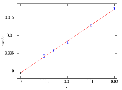
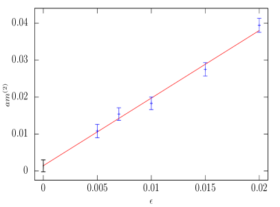
Figure 1: (Color online) An example of the extrapolation to $\epsilon\rightarrow 0$ of the unimproved bare PCAC quark mass in lattice units at the first (left) and second loop (right) in powers of $\beta^{-1/2}$ with $N_{S}=24$. In both panels the black, leftmost point represents the extrapolated result, the points in blue the results at finite $\epsilon$ obtained with the NSPT simulations while the red, continuous line corresponds to the fit function.

$N_{S}$		$\epsilon$
		0.005		0.007		0.010		0.015		0.020
11		21.2		19.8		19.7		19.7		19.7
12		20.4		18.0		25.2		19.7		18.9
13		19.8		21.8		19.8		24.8		19.3
14		19.0		29.9		27.9		28.1		28.2
15		18.5		18.0		18.0		19.5		18.0
16		17.9		18.1		18.0		17.9		18.8
17		18.8		18.6		18.9		18.3		17.9
18		17.3		15.8		17.6		13.3		17.0
20		13.5		13.1		15.4		13.3		12.8
24		12.6		13.3		12.8		13.3		13.4
32		3.3		3.3		3.0		2.8		2.6

Table 1: Number of measurements (in tens of thousands) of $f_{A}$ and $f_{P}$ for the different combinations of simulation parameters ($N_{S}$,$\ \!\epsilon$).

$N_{S}$		$am^{(1)}$		$am^{(2)}$		$a\delta m^{(0)}$​		$a\delta m^{(1)}$   ​
11		0.0031(2)		0.0048(04)		0.0711		-0.0460(65)
12		0.0029(3)		0.0021(16)		0.0598		-0.0494(64)
13		0.0025(5)		0.0018(28)		0.0510		-0.0408(51)
14		0.0018(3)		0.0032(18)		0.0440		-0.0307(67)
15		0.0013(2)		0.0062(21)		0.0383		-0.0192(55)
16		0.0011(5)		0.0006(10)		0.0337		-0.0134(25)
17		0.0017(6)		0.0043(32)		0.0298		-0.0148(60)
18		0.0012(3)		0.0003(14)		0.0266		-0.0083(17)
20		0.0002(5)		0.0039(17)		0.0216		-0.0013(37)
24		-0.0005(3)		0.0014(16)		0.0150		-0.0006(31)
32		0.0017(7)		-0.0003(38)		0.0084		0.0060(46)

Table 2: $\epsilon\rightarrow 0$ results for the one- and two-loop contribution $m^{(1)}$ and $m^{(2)}$ to the unimproved PCAC quark mass and for the improvement mass term at tree level ($\delta m^{(0)}$) and first-loop order ($\delta m^{(1)}$) for the values of $N_{S}$ used in this study: all these quantities are here expressed in lattice units. The values in brackets correspond to the statistical error affecting all observables but those at tree level as explained in footnote 8. The perturbative expansion all these observables are associated to is in powers of $\beta^{-1/2}$.

Data analysis and results - Simulations were performed with the following values of the parameters: $\theta=1.2$, $\epsilon\in\{0.005,0.007,0.010,0.015,0.020\}$ and $N_{S}\in\{11,12,13,14,15,16,17,18,20,24,32\}$. Note that, since the Euler scheme is employed in the integration of the Langevin equation, only three values of $\epsilon$ would be actually needed to extrapolate to $\epsilon\rightarrow 0$. However, we used $5$ time steps in order to increase the precision of the extrapolation. In our analysis we did not make use of the data obtained from the simulations featuring $N_{S}$ lower than $11$ since such data turned out to be rather noisy — this phenomenon is actually puzzling and, unfortunately, we have to admit that we could not find any convincing explanation for it.
Tab.(1) details the number of measurements of observables $f_{A}$ and $f_{P}$ in Eqs.(23) — and, hence, of the unrenormalized PCAC quark mass — for the different combinations of simulation parameters $(N_{s},\epsilon)$. For each setup two subsequent measurements were separated by 100 Langevin updates of the lattice configuration in order to reduce the autocorrelation. It is worth stressing that these 100 updating steps usually took approximately half of the time needed to perform a single measurement of the bare PCAC quark mass.
Fig.(1) shows a plot of the unimproved bare PCAC quark mass in lattice units — see Eq.(24) for its definition in physical units — at the first ($am^{(1)}$) and second loop ($am^{(2)}$) in powers of $\beta^{-1/2}$ vs. $\epsilon$ together with the extrapolated result. Statistical errors on the data in blue in Fig.(1) have been obtained through a jackknife procedure.
Before computing $c_{A}^{(2)}$, we check to which extent our approach is reliable: it is understood that all bare PCAC quark masses referred to in the rest of this section are obtained from an extrapolation to $\epsilon\rightarrow 0$ as that shown in Fig.(1).
As a first test, we compared the analytical result for the tree-level bare PCAC quark mass in lattice units Luscher et al. (1996) with our estimate. The two values agree apart from round-off errors that are usually lower than $0.03\%$ — the smallest tree-level bare PCAC quark mass we measure is equal to $2.97\cdot 10^{-6}$ for $N_{S}=32$, which is also the extent where round-off errors turn out to be the largest.
As a second check, we now work out the one-loop coefficient $c_{A}^{(1)}$ and compare it to the value determined in Luscher et al. (1996). To better explain the fit strategy, we rewrite the product of the lattice extent $L_{S}$ times the improved bare PCAC quark mass $m_{imp}$ in Eq.(25) as

$$m_{imp}L_{S}=(m+c_{A}\delta m)L_{S}\ ,\vspace*{0.3cm}$$ (44)

where $m$ is defined in Eq.(24) and $a$ has been set to $1$ — let us recall once more that any dependence in the lattice spacing is purely formal. Plugging Eq.(19) into the previous formula, at one-loop level we have

$$m_{imp}^{(1)}L_{S}=(m^{(1)}+c_{A}^{(1)}\delta m^{(0)})L_{S}\ .\vspace*{0.3cm}$$ (45)

$\delta m^{(0)}$ corresponds to the tree-level contribution to the term (including the denominator) multiplied times $c_{A}$ on the r.h.s. of Eq.(25): being a quantity at tree level, it bears no error.

In order to determine $c_{A}^{(1)}$, we proceed as follows: tentative values $\tilde{c}_{A}^{\ \!\!(1)}$’s are assigned to $c_{A}^{(1)}$, $m_{imp}^{(1)}L_{S}$ is fitted vs. $f(1/N_{S})=d\frac{1}{N_{S}}$ and any $\tilde{c}_{A}^{\ \!\!(1)}$ is eventually retained as valid if the coefficient $d$ is compatible with $0$ within errorbars. In this way, we obtain a range $[\tilde{c}_{A,min}^{\ \!\!(1)},\tilde{c}_{A,max}^{\ \!\!(1)}]$ of valid values for $c_{A}^{(1)}$ and we quote as mean value $\overline{c}_{A}^{(1)}$ and statistical error $\sigma_{c_{A}^{(1)}}$ on this one-loop improvement coefficient the expressions

$$\overline{c}_{A}^{(1)}=\frac{\tilde{c}_{A,min}^{\ \!\!(1)}+\tilde{c}_{A,max}^{\ \!\!(1)}}{2}\ ,\ \ \ \sigma_{c_{A}^{(1)}}=\frac{\tilde{c}_{A,max}^{\ \!\!(1)}-\tilde{c}_{A,min}^{\ \!\!(1)}}{2}\ .\vspace*{0.4cm}$$ (46)

As for the systematic error, its main source is given by the truncation of function $f(1/N_{S})$ at the first order in $1/N_{S}$. Therefore, the best way to assess the systematics would be to repeat the procedure above with a function of higher order in $1/N_{S}$ and to compare the outcome with that obtained with a linear function. In fact, as pointed out in Luscher et al. (1996), for relatively large values of $\theta$ as that used in this study, corrections going like $1/N_{S}^{2}$ can be comparable to the leading contribution $1/N_{S}$. Unfortunately, our data are not precise enough to support higher-order terms in $f(1/N_{S})$: any attempt of fit in this sense winds up with an extremely poor determination of $c_{A}^{(1)}$. In order to assess the systematic error in a somehow coarser way, we carried out the fit of $m_{imp}^{(1)}L_{S}$ vs. $f(1/N_{S})=d\frac{1}{N_{S}}$ as before but within a range of $N_{S}$ limited to the three smallest extents (i.e., $N_{S}\in[11,13]$). Since the latter is the regime where higher-order corrections in $N_{S}$ should have more impact, the mean value of $c_{A}^{(1)}$ obtained in this way should feature the largest deviation with respect to the mean value of $c_{A}^{(1)}$ computed with the fit employing all available sizes. Such a deviation could then be considered as a rough estimate of the systematic error.

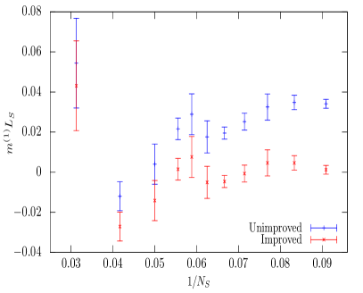
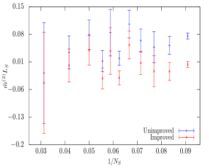
Figure 2: (Color online) Plots of $m^{(1)}L_{S}$ (left, in blue) and $\tilde{m}^{(2)}L_{S}$ (right, in blue) – as referred to on the r.h.s. of Eqs.(45) and (48) respectively — vs. $1/N_{S}$. The points in red denoted with stars correspond to their improved counterparts — referred to on the l.h.s. of the same equations — where $c_{A}^{(1)}$ on the left and $c_{A}^{(2)}$ on the right have been set to the mean values reported in Eqs.(47) and (49) respectively (with a conversion from powers of $g_{0}$ to powers of $\beta^{-1/2}$ properly taken into account). Observables in both panels refer to a perturbative expansion in $\beta^{-1/2}$ and can be computed starting from the values in Tab.(2).

Following this strategy and converting our expansion in $\beta^{-1/2}$ into a series in $g_{0}$, the result we obtain for $c_{A}^{(1)}$ reads

$$c_{A}^{(1)}=-0.00701(53)(50)\ ,\vspace*{0.2cm}$$ (47)

where the first and second error are the statistical and systematic uncertainty respectively. Within errorbars, this values is in reasonable agreement with $c_{A}^{(1)}=-0.00756(1)$ quoted in Luscher et al. (1996), though the precision of the latter estimate is much higher than that obtained with NSPT.

If we now move to the evaluation of $c_{A}^{(2)}$, we can first write the counterpart of Eq.(45), i.e.,

$$\begin{split}m_{imp}^{(2)}L_{S}&=(m^{(2)}+c_{A}^{(1)}\delta m^{(1)}+c_{A}^{(2)}\delta m^{(0)})L_{S}=\ \\ &=(\tilde{m}^{(2)}+c_{A}^{(2)}\delta m^{(0)})L_{S}\ ,\\ &\end{split}$$ (48)

where $c_{A}^{(1)}$ has been set to its known value $c_{A}^{(1)}=-0.00756$. Starting from the last expression, the same procedure adopted at one-loop level can be applied to the fit of $m_{imp}^{(2)}L_{S}$ with respect to $1/N_{S}$, only $m^{(1)}$ in Eq.(45) has to be replaced with $\tilde{m}^{(2)}=m^{(2)}+c_{A}^{(1)}\delta m^{(1)}$. Similarly to what remarked before for $\delta m^{(0)}$, $\delta m^{(1)}$ corresponds to the one-loop contribution to the term (including the denominator) multiplied times $c_{A}$ on the r.h.s. of Eq.(25).

After converting again the expansion in $\beta^{-1/2}$ into a series in $g_{0}$, the result we get for $c_{A}^{(2)}$ is

$$c_{A}^{(2)}=-0.00256(22)(6)\ .\vspace*{0.2cm}$$ (49)

While at one loop the systematic error is essentially equal to the statistical one, at two-loop level systematic effects seem to be apparently less important. This is most likely a consequence of a worse signal-to-noise ratio at the second loop, as shown in Fig.(2) where $m^{(1)}L_{S}$ and $\tilde{m}^{(2)}L_{S}$ are plotted – together with their $\emph{O}(a)-$improved counterparts — on the left and right panel respectively. At one loop, statistical errors are smaller and, consequently, the trend of the data is altogether better defined, thus allowing for the rough assessment of subleading corrections in $1/N_{S}$ outlined above. On the contrary, at two-loop level the trend of the data is harder to be determined due to the larger errorbars: this eventually leads to a more difficult estimate of the impact of subleading contributions in $1/N_{S}$ and, in practice, to an apparently small systematics.
In order to be somehow more conservative, we assume the systematic error at two-loop level to be roughly comparable to the statistical uncertainty, as it is the case for the first-loop result in Eq.(47). In this spirit, the estimate for $c_{A}^{(2)}$ would read

$$c_{A}^{(2)}=-0.00256(22)(20)\ .\vspace*{0.2cm}$$ (50)

For completeness, in Tab.(2) we provide — for the different values of $N_{S}$ — the $\epsilon\rightarrow 0$ results for $m^{(1)}$, $m^{(2)}$, $\delta m^{(0)}$ and $\delta m^{(1)}$ (in lattice units), i.e., all the mass contributions entering the computation of $c_{A}^{(1)}$ and $c_{A}^{(2)}$ explained in this section.

Conclusions - By studying the cutoff dependence of the unrenormalized PCAC quark mass, we carried out an exploratory, perturbative determination of the improvement coefficient $c_{A}$ to two loops by using NSPT in the quenched approximation. The crosschecks at zero- and one-loop in PT reproduce — with fair precision — results previously obtained in other independent studies, thus indicating that NSPT can in principle be used in this kind of computations, even at orders where non-numerical approaches are usually too cumbersome from an algebraic point of view. Let us recall that the loop $N_{L}$ at which the Taylor series in Eqs.(40) are truncated is in fact just a parameter and increasing it does not entail any extra work from the point of view of computer coding.

However, though viable in theory, at a practical level NSPT seems to be very demanding in terms of computer resources when it comes to producing an accurate estimate of the improvement coefficients, even in a relatively simple setup as that examined in this study, featuring the quenched approximation and the Wilson action at two loops. Indeed, in spite of having employed some millions of CPU hours, data are still rather noisy, as shown in Fig.(2): though not optimal at the first loop already (and, in fact, our estimate for $c_{A}^{(1)}$ is much less precise than that contained in Luscher et al. (1996)), the deterioration of the signal at higher order in PT is manifest and gets particularly reflected in a difficult assessment of the systematic uncertainty. It might be that observables other than that examined in this study — i.e., the unrenormalized PCAC quark mass — display an intrinsically better signal-to-noise ratio but, at present, we would have no suggestion to make with respect to this issue.
Our understanding is that reducing errorbars to a level at which NSPT data can be accurately fitted (and improvement coefficients precisely determined) would most likely require considerable computer resources irrespective of the quantity being monitored, especially if higher order in PT are envisaged and/or more interesting — but also more demanding — setups are considered, as that of unquenched simulations.
More or less recently, some works have actually been published Luscher et al. (2017); Dalla Brida et al. (2017, 2017) proposing some technical changes to the standard NSPT approach followed in this study. Such changes yield new setups — called Instantaneous Stochastic Perturbation Theory (ISPT), Hybrid Stochastic Perturbation Theory (HSPT) and Kramers Stochastic Perturbation Theory (KSPT) — that seem to be highly beneficial in remeding the shortcomings of the standard version of NSPT we employed: this looks particularly true for the formulation described in Dalla Brida et al. (2017). It would be extremely interesting to carry out a computation of $c_{A}^{(2)}$ with the latter setup in order to (hopefully) get a more precise estimate of this improvement coefficient at much lower computer costs.

Nevertheless, we believe that the original result of this project, i.e., the evaluation of the coefficient $c_{A}^{(2)}$ for $N_{f}=0$, can serve as a benchmark to some extent: indeed, we are confident that at least its negative sign and its order of magnitude (that is, $10^{-3}$) are reliable.

Acknowledgements - We would like to thank G.S. Bali for useful discussions at different stages of this project. Simulations were carried out on the Athene cluster of the University of Regensburg and on the cluster of the Leibniz-Rechenzentrum in Munich.

This work is dedicated to my wife, Milena, and to our sons, Edoardo and Martino.

References

- Ukawa (2002) A. Ukawa, Nucl. Phys. Proc. Suppl. 106, 195 (2002).
- Borsanyi et al. (2015) S. Borsanyi, S. Durr et al., Science 347, 1452 (2015), arXiv:1406.4088 [hep-lat] .
- Duane et al. (1987) S. Duane, A. D. Kennedy, B. J. Pendleton, and D. Roweth, Phys. Lett. B195, 216 (1987) .
- DeGrand et al. (1987) T. A. DeGrand and P. Rossi, Comput. Phys. Commun. 60, 211 (1990) .
- Hasenbusch (2001) M. Hasenbusch, Phys. Lett. B519, 177 (2001), arXiv:hep-lat/0107019 [hep-lat] .
- Sexton et al. (1992) J. C. Sexton and D. H. Weingarten, Nucl. Phys. B380, 665 (1992) .
- Albanese et al. (1987) M. Albanese et al., Phys. Lett. B192, 163 (1987) .
- Hasenfratz et al. (2001) A. Hasenfratz and F. Knechtli, Phys. Rev. D64, 034504 (2001), arXiv:hep-lat/0103029 [hep-lat] .
- Morningstar et al. (2004) C. Morningstar and M. J. Peardon, Phys. Rev. D69, 054501 (2004), arXiv:hep-lat/0311018 [hep-lat] .
- Capitani et al. (2006) S. Capitani, S. Durr, and C. Hoelbling, JHEP 11, 028 (2006), arXiv:hep-lat/0607006 [hep-lat] .
- Symanzik (1983) K. Symanzik, Nucl. Phys. B226, 187 (1983) .
- Sheikholeslami et al. (1985) B. Sheikholeslami and R. Wohlert, Nucl. Phys. B259, 572 (1985) .
- Di Renzo et al. (1994) F. Di Renzo, E. Onofri, G. Marchesini, and P. Marenzoni, Nucl. Phys. B426, 675 (1994), arXiv:hep-lat/9405019 [hep-lat] .
- Di Renzo et al. (2004) F. Di Renzo and L. Scorzato, JHEP 10, 073 (2004), arXiv:hep-lat/0410010 [hep-lat] .
- Sint (1994) S. Sint, Nucl. Phys. B421, 135-158 (1994), arXiv:hep-lat/9312079 [hep-lat] .
- Luscher et al. (1992) M. Luscher, R. Narayanan, P. Weisz, and U. Wolff, Nucl. Phys. B384, 168 (1992), arXiv:hep-lat/9207009 [hep-lat] .
- Luscher et al. (1996) M. Luscher, S. Sint, R. Sommer, and P. Weisz, Nucl. Phys. B478, 365 (1996), arXiv:hep-lat/9605038 [hep-lat] .
- Luscher et al. (1985) M. Luscher and P. Weisz, Phys. Lett. B158, 250 (1985) .
- Wohlert (1987) R. Wohlert, unpublished (1987) .
- Luscher et al. (1996) M. Luscher and P. Weisz, Nucl. Phys. B479, 429 (1996), arXiv:hep-lat/9606016 [hep-lat] .
- Aoki et al. (2003) S. Aoki and Y. Kuramashi, Phys. Rev. D68, 094019 (2003), arXiv:hep-lat/0306015 [hep-lat] .
- Horsley et al. (2008) R. Horsley, H. Perlt, P. E. L. Rakow, G. Schierholz, and A. Schiller, Phys. Rev. D78, 054504 (2008), arXiv:0807.0345 [hep-lat] .
- Panagopoulos et al. (2003) H. Panagopoulos and Y. Proestos, Phys. Rev. D65, 014511 (2002), arXiv:hep-lat/0108021 [hep-lat] .
- Heatlie et al. (1991) G. Heatlie, G. Martinelli, C. Pittori, G. C. Rossi, and C. T. Sachrajda, Nucl. Phys. B352, 266 (1991) .
- Parisi et al. (1980) G. Parisi and Y.-s Wu, Sci. Sin. 24, 483 (1981) .
- Aarts et al. (2017) G. Aarts, E. Seiler, D. Sexty, and I.-O. Stamatescu, JHEP 05, 044 (2017), arXiv:1701.02322 [hep-lat] .
- Di Renzo et al. (2015) F. Di Renzo and G. Eruzzi, Phys. Rev. D92, 085030 (2015), arXiv:1507.03858 [hep-lat] .
- Floratos et al. (1983) E. Floratos and J. Iliopoulos, Nucl. Phys. B214, 392 (1983), arXiv:1507.03858 [hep-lat] .
- Drummond et al. (1983) I. T. Drummond, S. Duane, and R. R. Horgan, Nucl. Phys. B220, 119 (1983) .
- Di Renzo et al. (2004) F. Di Renzo, A. Mantovi, V. Miccio, and Y. Schroder, JHEP 05, 006 (2004), arXiv:hep-lat/0404003 .
- Di Renzo et al. (2006) F. Di Renzo, M. Laine, V. Miccio, Y. Schroder, and C. Torrero, JHEP 07, 026 (2006), arXiv:hep-ph/0605042 .
- Di Renzo et al. (2008) F. Di Renzo, M. Laine, Y. Schroder, and C. Torrero, JHEP 09, 061 (2008), arXiv:0808.0557 [hep-lat] .
- Di Renzo et al. (2006) F. Di Renzo, V. Miccio, L. Scorzato, and C. Torrero, Eur. Phys. J. C51, 645-657 (2007), arXiv:hep-lat/0611013 .
- Di Renzo et al. (2010) F. Di Renzo, E.-M. Ilgenfritz, H. Perlt, A. Schiller, and C. Torrero, Nucl. Phys. B831, 262-284 (2010), arXiv:0912.4152 [hep-lat] .
- Di Renzo et al. (2011) F. Di Renzo, E.-M. Ilgenfritz, H. Perlt, A. Schiller, and C. Torrero, Nucl. Phys. B842, 122-139 (2011), arXiv:1008.2617 [hep-lat] .
- Brambilla et al. (2013) M. Brambilla and F. Di Renzo, Eur. Phys. J. C73, 2666 (2013) no. 12, arXiv:1310.4981 [hep-lat] .
- Brambilla et al. (2013) M. Brambilla, F. Di Renzo and M. Hasegawa, Eur. Phys. J. C74, 2944 (2014) no. 7, arXiv:1402.6581 [hep-lat] .
- Di Renzo et al. (1995) F. Di Renzo, E. Onofri, and G. Marchesini, Nucl. Phys. B457, 202-216 (1995), arXiv:hep-th/9502095 .
- Di Renzo et al. (2001) F. Di Renzo and L. Scorzato, JHEP 10, 038 (2001), arXiv:hep-lat/0011067 .
- Bali et al. (2013) G. S. Bali, C. Bauer, A. Pineda, and C. Torrero, Phys. Rev. D87, 094517 (2013), arXiv:1303.3279 [hep-lat] .
- Bali et al. (2014) G. S. Bali, C. Bauer, and A. Pineda, Phys. Rev. D89, 054505 (2014), arXiv:1401.7999 [hep-ph] .
- Bali et al. (2014) G. S. Bali, C. Bauer, and A. Pineda, Phys. Rev. Lett. 113, 092001 (2014), arXiv:1403.6477 [hep-ph] .
- Del Debbio et al. (2018) L. Del Debbio, F. Di Renzo, and G. Filaci, arXiv:1807.09518 [hep-lat] .
- Zwanziger (1981) D. Zwanziger, Nucl. Phys. B192, 259 (1981) .
- Brambilla et al. (2013) M. Brambilla, M. Dalla Brida, F. Di Renzo, D. Hesse, and S. Sint, PoS Lattice2013, 325 (2014), arXiv:hep-lat/1310.8536 .
- Rossi et al. (1988) P. Rossi, C. T. H. Davies, and G. P. Lepage, Nucl. Phys. B297, 287 (1988) .
- Luscher et al. (2017) M. Luscher, JHEP 04, 142 (2015), arXiv:1412.5311 [hep-lat] .
- Dalla Brida et al. (2017) M. Dalla Brida, M. Garofalo, and A. D. Kennedy, Phys. Rev. D96, 054502 (2017) no. 5, arXiv:1703.04406 [hep-ph] .
- Dalla Brida et al. (2017) M. Dalla Brida and M. Luscher, Eur. Phys. J. C77, 308 (2017) no. 5, arXiv:1703.04396 [hep-lat] .