Semantic DMN: Formalizing and Reasoning About Decisions in the Presence of Background Knowledge

Abstract

The Decision Model and Notation (DMN) is a recent OMG standard for the elicitation and representation of decision models, and for managing their interconnection with business processes. DMN builds on the notion of decision tables, and their combination into more complex decision requirements graphs (DRGs), which bridge between business process models and decision logic models. DRGs may rely on additional, external business knowledge models, whose functioning is not part of the standard. In this work, we consider one of the most important types of business knowledge, namely background knowledge that conceptually accounts for the structural aspects of the domain of interest, and propose decision knowledge bases (DKBs), which semantically combine DRGs modeled in DMN, and domain knowledge captured by means of first-order logic with datatypes. We provide a logic-based semantics for such an integration, and formalize different DMN reasoning tasks for DKBs. We then consider background knowledge formulated as a description logic ontology with datatypes, and show how the main verification tasks for DMN in this enriched setting can be formalized as standard DL reasoning services, and actually carried out in ExpTime. We discuss the effectiveness of our framework on a case study in maritime security.

1 Introduction

The Decision Model and Notation (DMN) is a recent OMG standard for the representation and enactment of decision models [OMG (2016)]. The standard proposes a model and notation for capturing single decision tables as well as the interconnection of multiple decision tables and their relationship with other forms of business knowledge. In addition, it proposes a clean integration with business process models, with particular reference to BPMN, so as to achieve a suitable separation of concerns between the process logic and the decision logic [Batoulis et al. (2015)].

For all these reasons, the standard has attracted the attention of both academia and industry, giving a new momentum to the field of decision and rule management and its interplay with business process management. The standard is already receiving widespread adoption in the industry, and an increasing number of tools and techniques are being developed to assist users in modeling, verifying, and applying DMN models. This is, e.g., witnessed by the incorporation of DMN inside the Signavio toolchain for business process management, and inside the open-source OpenRules business rules and decision management system.

DMN builds on the notion of decision table, defined as “the act of determining an output value (the chosen option), from a number of input values, using logic defining how the output is determined from the inputs” [OMG (2016)]. This is diagrammatically related to the long-standing notion of decision table [Pooch (1974), Vanthienen and Dries (1993)], which consists of columns representing the inputs and outputs of a decision, and rows denoting rules. Concretely, DMN comes with two languages for capturing the decision logic. The most sophisticated language, called FEEL (Friendly Enough Expression Language), is a complex, textual specification language not apt to be used and understood by domain experts, and that does not come with a graphical notation. It is Turing-powerful since it relies on various mechanisms to specify rules using complex arithmetic expressions and generic functions, in turn expressed in FEEL itself or in external languages such as Java. The second decision logic specification language supported by DMN, the one we are actually considering in this paper, is called S-FEEL (Simplified-FEEL). S-FEEL is equipped with a graphical notation that is also defined in the standard. It is a simple rule-based language that employs comparison operators between attributes and constants as atomic expressions, which are then combined into more general conditions using boolean operators (with a restricted usage of negation). Interestingly, S-FEEL emerged as a suitable trade-off between expressiveness and simplicity, and its main principles come from previous, long-standing research in decision and rule management (e.g., a very similar language is adopted in the well-established Prologa tool).

While DMN decision tables are rooted in mainstream approaches to decision management, a distinctive feature of the DMN standard itself is the combination of multiple decision tables into more complex so-called decision requirements graphs (DRGs), graphically depicted using decision requirements diagrams (DRDs). DRGs provide “a bridge between business process models and decision logic models” [OMG (2016)]: for every task in the process model of interest where decision-making is required, a dedicated DRG provides a separate definition of which decisions must be made within such a task, together with the interrelationships of such decisions, and their requirements for decision logic. In particular DRGs may rely on additional so-called business knowledge models for their functioning. Business knowledge models are external to the DRG, and consequently the standard does not dictate how they should be specified, nor how they semantically interact with the internal decision logic expressed by the DRG.

In this work, we consider one of the most important types of business knowledge, namely background knowledge that conceptually accounts for the relevant, structural aspects of the domain of interest (such as entities and their main relationships). As customary, we assume that this background knowledge is explicitly encapsulated inside an ontology. The main issue that arises when a DRG is integrated with an ontology is that the DRG should not any longer be interpreted under the assumption of complete information. Interestingly, this does not only affect the way the DRG is applied on specific input data to compute corresponding outputs, but also impacts on the intrinsic properties of the DRG, such as completeness (defined as the ability of “providing a decision result for any possible set of values of the input data” [OMG (2016)]). To tackle this fundamental challenge, we introduce a combined framework, called semantic DMN, based on the notion of decision knowledge base (DKB). A DKB semantically combines a decision logic, modeled as a DMN DRG whose decision tables are expressed in S-FEEL, with a general ontology formalized using multi-sorted first-order logic. The different sorts are used to seamlessly integrate abstract domain objects with data values belonging to the concrete domains used in the DMN rules (such as strings, integers, and reals).

We provide a logic-based semantics for DKBs, thus proposing, to the best of our knowledge, the first formalization of DRGs and of their integration with background knowledge. Due to the specific challenges posed by such an integration, the formalization of the DMN decision tables contained in the DRG is of independent interest, and represents a conceptual refinement of the logic-based formalization proposed by CDL16. We then approach the problem of actually reasoning on DKBs, on the one hand providing a formalization of the most fundamental reasoning tasks, and on the other hand giving insights on how they can be actually carried out, and with which complexity. To this end, we need to restrict the expressive power of the ontology language. In fact, we target the significant case where the ontology consists of a description logic (DL) [Baader et al. (2007)] knowledge base equipped with datatypes [Lutz (2002b), Savkovic and Calvanese (2012), Artale et al. (2012), Bao et al. (2012)]. In such a DL, besides the domain of abstract objects, one can refer to concrete domains of data values (such as strings, integers, and reals) accessed through functional relations. Complex conditions on such values can be formulated by making use of unary predicates over the concrete domains. The restriction to unary predicates only, is what distinguishes DLs with datatypes from the richer setting of DLs with concrete domains, where in general arbitrary predicates over the datatype/concrete domain can be specified. We demonstrate that these constructs are expressive enough to encode DRGs.

Then, we exploit this encoding to show that all the introduced reasoning tasks can be decided in ExpTime in the case where background knowledge is represented using the DL $\mathsf{ALCH}(\mathfrak{D})$. This DL is a strict sub-language of the ontology language OWL 2, which has been standardized by the W3C [Bao et al. (2012)], hence one can rely on standard OWL 2 reasoners [Tsarkov and Horrocks (2006), Sirin and Parsia (2006), Shearer et al. (2008)] for all reasoning tasks in $\mathsf{ALCH}(\mathfrak{D})$ and on DKBs. However, this does not provide us with computationally optimal complexity bounds. On the one hand, while OWL 2 and $\mathsf{ALCH}(\mathfrak{D})$ are equipped with multiple datatypes (which is also indicated by the letter $\mathfrak{D}$ in the name of the latter logic), reasoning in the very expressive DL $\mathit{SROIQ}(D)$, which is the formal counterpart of OWL 2, was initially studied for a single datatype only (which is indicated by the letter $D$ in the name) [Horrocks et al. (2006)]. As pointed out already by HoKS06, the proposed reasoning technique can be extended to multiple datatypes by following the proposal by PaHo03. Still, the adopted algorithms are tableaux-based, and while typically effective in practical scenarios, they do not provide worst-case optimal computational complexity bounds [Baader and Sattler (2000)]. To show that reasoning in $\mathsf{ALCH}(\mathfrak{D})$ can indeed be carried out in worst-case single exponential time, we develop a novel algorithm that is based on the knot technique proposed by OrSE08 for query answering in expressive DLs.

To introduce the main motivations behind our proposal and show its effectiveness, we consider a complex case study in maritime security extracted from one of the challenges of the decision management community, arguing that our approach facilitates modularity, separation of concerns, and understanding of how a decision logic can be contextualized in a specific setting.

This article is an extended version of an article by CDMM17. Differently from that work, we consider here the new version of the standard (i.e., DMN 1.1), and we deal not only with single decision tables, but also with their interconnection in a DRG. By considering DRGs, we extend the logic-based formalization proposed by CDMM17, expand our case study accordingly, and introduce new interesting properties that refer to the overall decision logic encapsulated in a DRG.

The article is organized as follows. In Section 2 we present the case study in maritime security. In Section 3 we introduce the two formalism we use in our formalization of DMN DRGs, namely multi-sorted first-order logic, and DLs extended with datatypes, and we define DMN decision tables according to DMN 1.1. In Section 4 we introduce and formalize DKBs, and discuss the reasoning tasks over them. In Section 5 we address the problem of reasoning over DKBs by resorting to a translation in DLs. In Section 6 we discuss related work, and in Section 7 we draw final conclusions.

2 Case Study

Our case study is inspired by the international Ship and Port Facility Security Code, used by port authorities to determine whether a (cargo) ship can enter a Dutch port. On the one hand, this requires to decide ship clearance, that is, whether a ship approaching the port can enter or not. On the other hand, we also consider the communication of where the refueling station is located for the approaching ship. Both such interrelated decisions depend on a combination of ship-related data, some focusing on the physical characteristics of the ship, and others on contingent information such as the transported cargo and certificates exhibited by the owner of the ship.

2.1 Domain Description

To describe how ship clearance is handled by a port authority, three main knowledge models, reported in Figure 1, have to be suitably integrated:

• background domain knowledge, describing the different types of cargo ships and their physical characteristics (see Figure 1(c));

• the clearance process, describing when clearance has to be assessed, how the different clearance-related tasks can unfold over time, which data must be collected, and which possible ending states exist (see Figure 1(a));

• the clearance decision, capturing the decision logic that relates all the important ship data with the determination of whether the ship can enter or not, and where its refuel station is located (see Figure 1(b)).

It is important to notice that the different knowledge models are not necessarily developed and maintained by the same responsible authority, nor co-evolve in a synchronous way. For example, the background knowledge may be obtained by combining the catalogues produced by the different ship vendors, and updated when vendors change the physical characteristics of the types of ship they produce. The process may vary from port to port, still ensuring that its functioning behaves in accordance with national regulations. Finally, the clearance decision may contain decisions with different authorities: the decision of whether a ship can enter into a port or not may be in fact handled at the national level, keeping it aligned with the evolution of laws and norms, whereas the determination of the refuel area may vary from port to port, so as to reflect its physical characteristics and internal operational rules.

In the following, we detail each of the three knowledge models mentioned above.

Business process.  The process adopted by the port authority is shown in Figure 1(a) using the BPMN notation. An instance of this process is created whenever an entrance request is received by the port authority from an approaching ship. The process management system immediately extracts the main data associated to the ship, namely its identification code, as well as its type. Then, two branches are executed in parallel. The first branch is about performing a physical inspection of the ship, in particular to determine the amount of cargo residuals carried by the ship. The second branch deals instead with the acquisition of the ship certificate of registry, in particular to extract its expiration date (for simplicity, we do not handle here the case where the ship does not own a valid certificate).

Once all these data are obtained, a business rule task is used to decide about whether the ship can enter into the port or not and, if so, where the refuel area for that ship is located. If the resulting decision concludes that the ship cannot enter, the process terminates by communicating the refusal to the ship. If instead the ship is allowed to enter, the dock is opened and the process terminates by informing the ship about the refuel area.

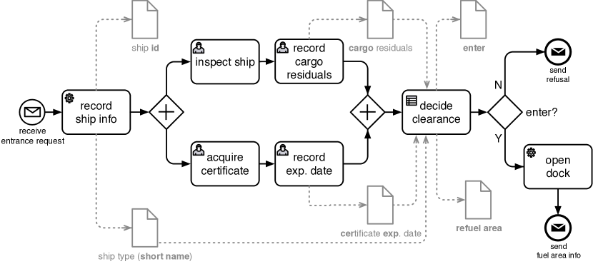
(a) BPMN process

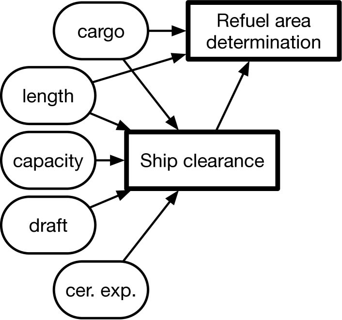
(b) DRD for decide clearance

Ship Type	Short Name	Length (m)	Draft (m)	Capacity (TEU)
Converted Cargo Vessel	CCV	135	0 – 9	500
Converted Tanker	CT	200	0 – 9	800
Cellular Containership	CC	215	10	1000 – 2500
Small Panamax Class	SPC	250	11 – 12	3000
Large Panamax Class	LPC	290	11 – 12	4000
Post Panamax	PP	275 – 305	11 – 13	4000 – 5000
Post Panamax Plus	PPP	335	13 – 14	5000 – 8000
New Panamax	NP	397	15.5	11000 – 14500

(c) Ontology of cargo ships and their physical characteristics

Figure 1: Three knowledge models used by a port authority to determine clearance and location of the refuel area for a ship: (a) captures the business process using BPMN; (b) shows a DMN DRD encapsulating the decision logic underlying the decide clearance business rule task used in the process; the decision logic has to be understood in the context of the ship ontology depicted in (c), which provides the background knowledge to understand the relationship between ship types and their corresponding characteristics. The ship ontology is hence depicted as a business knowledge model in the DRD.

Background domain knowledge.  In our setting, we consider background knowledge describing the different types of ships that may enter the port, together with their physical characteristics:

• length of the ship (in $m$);

• draft size (in $m$);

• capacity of the ship (in $\mathit{TEU}$, which stands for Twenty-foot Equivalent Units).

The taxonomy of ship types, together with the relationship between types and physical characteristics, is captured in a ship ontology, depicted in Table 1(c) using an informal tabular format.

Decision logic.  The decision logic consists of two decision tables: a ship clearance decision table used to determine whether a ship can enter a port or not, and a refuel area determination decision table used to compute which refuel area should be used by a ship. As pointed out before, we assume that the first table is fixed nationally, while the second is defined on a per-port basis.

Let us first focus on ship clearance. A ship can enter the port only if the ship complies with the requirements of the inspection. This is the case if the ship is equipped with a valid certificate of registry, and the ship meets the safety requirements. The certificate of registry owned by the ship is considered valid if the certificate expiration date is after the current date. The rules for establishing whether a ship meets the safety requirements depend on the characteristics of the ship, and the amount of residual cargo present in the ship. The limitation concerning residuals is specified in terms of concentration per space unit, fixing thresholds that depend on the capacity of the ship. This is because residual cargo has to be manually inspected by the port authority. Thresholds are then put to limit the amount of resources and time for the inspection. In addition, the concentration limits vary depending on the ship capacity so as to level the maximum amount of overall residuals to be inspected, irrespectively of the ship type.

In particular, small ships (with maximum length 260 m and maximum draft 10 m) may enter provided that their capacity does not exceed 1000 TEU. Ships with a small length (maximum 260 m), medium draft comprised between 10 m and 12 m, and capacity not exceeding 4000 TEU, may enter only if the carried cargo residuals do not exceed 0.75 mg dry weight per cm². Ships of medium size (with length comprised between 260 m and 320 m excluded, and draft strictly bigger than 10 m and not exceeding 13 m), and with a cargo capacity below 6000 TEU, may enter only if their cargo residuals do not exceed 0.5 mg dry weight per cm². Finally, big ships with length comprised between 320 m and 400 m excluded, draft larger than 13 m, and capacity exceeding 4000 TEU, may enter only if their carried residuals are at most 0.25 mg dry weight per cm². Larger ships are not explicitly mentioned in the rules, and are therefore implicitly considered as not eligible for entering.

Let us now focus on the determination of the refuel area. This decision table depends on ship clearance, and on some of the physical characteristics of the ship, in particular length and draft size. On the one hand, if clearance is rejected, then no area is assigned (this is represented using string $\mathtt{none}$). On the other hand, the $\mathtt{indoor}$ refuel area is preferred over the $\mathtt{outdoor}$ area, but it is not possible for too big ships to refuel indoor, due to physical constraints. In particular, ships that are longer than 350 m can only refuel indoor if their cargo does not carry more than 3 mg dry weight per cm².

2.2 Challenges

The first challenge posed by this case study concerns modeling, representation, management, and actual application of the clearance and refuel decision logic, as well as its integration with business processes. All these issues are tackled by the DMN standard. In particular, the standard defines clear guidelines on how to encode and graphically represent the input/output attributes and the rules of interest in the form of decision tables, as well as to aggregate them into a DRG that highlights how they interact with each other, and with other business knowledge models.

Specifically, the DRG of our case study is graphically rendered using the DRD of Figure 1(b). In this DRD:

• Rounded rectangles represent input data, to be assigned externally when the decision logic has to be applied in a specific context.

• Rectangles represent decision tables, which may require as input either input data provided externally, or the output produced by other decision tables; decision tables producing output results that must be returned to the external world are represented with bold contour (in our case study, both decision tables are of this form).

• Solid arrows represent information requirements, indicating which input data or decision tables are used as input to other decision tables.

• Rectangles with two clipped corners represent business knowledge models, which may be used by decision tables to properly compute their input-output relation (see Figure 4).

Additional constructs are available to interconnect different DRGs and describe authorities, i.e., sources of knowledge, but they are orthogonal to the core aspects introduced above, so we do not consider such additional constructs here.

Each DMN decision table can be decorated with meta-information capturing its hit policy, i.e., declare whether its contained rules are non-overlapping or, if they do, how to reconcile the output values produced by multiple rules that simultaneously trigger. In addition, both single decision tables and complete DRGs shall be understood in terms of their completeness, i.e., whether they are able to produce a final output for each possible configuration of the input data, or whether there are inputs for which the decision table is undefined. This is particularly critical in the case of DRGs, since incompleteness may be caused by internal mismatches between decision tables interconnected via information requirements. The main issue when it comes to such properties is that there is no guarantee that they are actually reflected by the actual decision logic [Calvanese et al. (2016)]. In addition, while these are the main properties mentioned by the DMN standard, there are many more properties that should be checked so as to ascertain the correctness of a DRG. For example, one could check whether all rules may potentially trigger. In the case of a single decision table this problem boils down to check whether certain rules are masked by others [Calvanese et al. (2016)]. However, in the more general case of a DRG, the fact that a rule never triggers may be related again to the complex interconnection among multiple decision tables.

The main point of this work, though, is that the investigation of such properties and, more in general, the meaning of a decision logic, cannot be understood in isolation from background knowledge, but has instead to be analyzed in the light of such knowledge. Conceptually, this requires to lift from an approach working under complete information to one that works under incomplete information, and where the background knowledge is used to constrain, complement, and contextualize the decision logic. This interplay is far from trivial, and impacts on the properties of a DRG and its contained decision tables, their input-output semantics as well as, ultimately, their correctness.

Here we discuss, using our case study, two of the most critical challenges when it comes to understand DMN in the presence of background knowledge. First and foremost, let us consider in more detail the interplay between the BPMN process in Figure 1(a), and the DRG in Figure 1(b). According to the standard, the integration between a process and a DRG is realized by introducing a business rule task in the process, then linking such a task to the DRG. This implicitly assumes a clear information exchange between these two knowledge models. On the one hand, when an instance of the business rule task is created in the context of a specific process instance, the input data of the DRG are bound to actual values obtained from the state process instance. On the other hand, the output values produced by the DRG are made visible to the process instance, which may rely on them to decide how to consequently route the instance.

In our case study, it is clear that, syntactically, the process and the DRG do not properly integrate with each other, in particular for what concerns the input data of the DRG. On the one hand, the DRG applies a comprehensive strategy, where all physical parameters of the ship are requested as input. On the other hand, the process adopts a pragmatic approach, in which only the ship type and the cargo residuals are recorded, without requiring the port personnel to measure each single physical parameter of the ship. While it is clear that a syntactic interconnection between the two knowledge models would not work, what about a semantic interconnection that considers the ship ontology as background knowledge? It turns out, interestingly, that once the ship ontology is inserted into the picture, the process and the DRG can properly interoperate. In fact, once the type of a ship is acquired, the ontology allows one to infer partial, but sufficient information about the physical characteristics of the ship, so as to properly apply the DRG once also the expiration date of the certificate, and the amount of cargo residuals, are obtained. It is worth noting that the ship ontology could not be reduced to an additional decision table component of the DRG: Table 1(c) is not a decision table, since it is not always possible to univocally compute the ship characteristics from the type (see, e.g., the case of Post Panamax ship type). In fact, the domain knowledge captured by Table 1(c) is a set of constraints, implicitly discriminating combinations of ship types and characteristics that are allowed from those that are impossible.

A second, open challenge relates to how the formal properties of single tables change when they are interconnected in a DRG, and/or interpreted in the presence of background knowledge. Consider the ship clearance decision table and its associated rules described above. By elaborating on such rules, one would conclude that such rules are non-overlapping, and that they are incomplete, since, e.g., they do not handle clearance of a long ship ($\geq$ 320 m) with small draft ($\leq$ 10 m). While the non-overlapping property clearly holds also when the ship ontology is considered, this is not the case for incompleteness. In fact, under the assumption that all possible ship types are those listed in Table 1(c), one would infer that all the allowed combinations of physical parameters as captured by the ontology are actually covered by the ship clearance decision table, which is in fact complete with respect to the ship ontology. E.g., the table clearly shows that the aforementioned combination of parameters is impossible: long ships cannot have such a small draft.

Finally, consider the decision table for refuel area determination. It is easy to see that the rules encapsulated in such a decision table are complete and non-overlapping. However, once this decision table is interconnected to ship clearance, it turns out that the $\mathtt{outdoor}$ station is never selected. In fact, such a station is selected for ships whose physical characteristics lead to reject the entrance request and, in turn, to be assigned to $\mathtt{none}$ refuel area independently of the actual physical characteristics.

Identifying all such issues is extremely challenging, and this is why we propose a framework that on the one hand formally defines the interplay between the different knowledge models, and on the other hand provides automated reasoning capabilities to actually check the overall properties of a DRG in the presence of background knowledge, as well as compute the consequences of a decision table when input data are only partially specified, if possible.

3 Sources of Decision Knowledge

We now generalize the case study presented in Section 2, and introduce the two main knowledge models of semantic DMN: background knowledge expressed using a logical theory enriched with datatypes, and decision logic captured as a DMN DRG.

3.1 Logics with Datatypes

To capture background knowledge, we resort to a variant of multi-sorted first-order logic (see, e.g., Ende01), which we call $\mathsf{FOL}(\mathfrak{D})$, where one sort $\Delta$ denotes a domain of abstract objects, while the remaining sorts represent a finite collection $\mathfrak{D}$ of datatypes. We consider a countably infinite set $\Sigma$ of predicates, where each $p\in\Sigma$ comes with an arity $n$, and a signature $\mathsf{Sig}_{p}:\{1,\ldots,n\}\rightarrow\mathfrak{D}\uplus\{\Delta\}$, mapping each position of $p$ to one of the sorts. $\mathsf{FOL}(\mathfrak{D})$ contains unary and binary predicates only. A unary predicate $N$ with $\mathsf{Sig}_{N}(1)=\Delta$ is called a concept, a binary predicates $P$ with $\mathsf{Sig}_{P}(1)=\mathsf{Sig}_{P}(2)=\Delta$ a role, and a binary predicate $F$ with $\mathsf{Sig}_{F}(1)=\Delta$ and $\mathsf{Sig}_{F}(2)\in\mathfrak{D}$ a feature.

Example 1.

The cargo ship ontology in Table 1(c) should be interpreted as follows: each entry applies to a ship, and expresses how the specific ship type constrains the other features of the ship, namely length, draft, and capacity. Thus the first table entry is encoded in $\mathsf{FOL}(\mathfrak{D})$ as

$$\forall s.\textsl{stype}(s,``CCV")\rightarrow\begin{array}[t]{@{}l}\textsl{Ship}(s)\land\forall\ell.(\textsl{length}(s,\ell)\rightarrow\ell=135)\land{}\\ \forall d.(\textsl{draft}(s,d)\rightarrow d\geq 0\land d\leq 9)\land\forall c.(\textsl{capacity}(s,c)\rightarrow c=500)\end{array}$$

where Ship is a concept, stype is a feature of sort string, while length, draft, and capacity are all features of sort real.  

We consider also well-behaved fragments of $\mathsf{FOL}(\mathfrak{D})$ that are captured by description logics (DLs) extended with datatypes. For details on DLs, we refer to BCMNP07, and for a survey of DLs equipped with datatypes (also called, in fact, concrete domain), to Lutz02d. Here we adopt the DL $\mathsf{ALCH}(\mathfrak{D})$, which is an extension of the well-known DL $\mathsf{ALC}(\mathit{D})$ [Lutz (2002b)] in two orthogonal directions: on the one hand $\mathsf{ALCH}(\mathfrak{D})$ allows one to express inclusions between two roles and between two features, which is denoted by the presence in the name of the logic of the letter $\mathsf{H}$, for role/features hierarchies; on the other hand, $\mathsf{ALCH}(\mathfrak{D})$ is equipped with multiple datatypes, instead of a single one. As for datatypes, we follow the proposal by MoHo08, on which the OWL 2 datatype maps are based [Motik et al. (2012), Section 4], but we adopt some simplifications that suffice for our purposes.

Datatypes.  A (primitive) datatype $D$ is a pair $\langle\Delta_{D},\Gamma_{D}\rangle$, where $\Delta_{D}$ is the domain of values of $D$, and $\Gamma_{D}$ is a (possibly infinite) set of facets, denoting unary predicate symbols. Each facet $S\in\Gamma_{D}$ comes with a set $S^{D}\subseteq\Delta_{D}$ that rigidly defines the semantics of $S$ as a subset of $\Delta_{D}$. Given a primitive datatype $D$, datatypes $E$ derived from $D$ are defined according to the following syntax

$$E~{}\longrightarrow~{}D~{}\mid~{}E_{1}\cup E_{2}~{}\mid~{}E_{1}\cap E_{2}~{}\mid~{}E_{1}\setminus E_{2}~{}\mid~{}\{\mathtt{v}_{1},\ldots,\mathtt{v}_{m}\}~{}\mid~{}D[S]$$

where $S$ is a facet for $D$, and $\mathtt{v}_{1},\ldots,\mathtt{v}_{m}$ are datatype values in $\Delta_{D}$. The domain of a derived datatype is obtained for $\cup$, $\cap$, and $\setminus$, by applying the corresponding set operator to the domains of the component datatypes, for $\{\mathtt{v}_{1},\ldots,\mathtt{v}_{m}\}$ as the set $\{\mathtt{v}_{1},\ldots,\mathtt{v}_{m}\}$, and for $D[S]$ as $S^{D}$. In the remainder of the paper, we consider the (primitive) datatypes present in the S-FEEL language of the DMN standard: strings equipped with equality, and numerical datatypes, i.e., naturals, integers, rationals, and reals equipped with their usual comparison operators (which, for simplicity, we all illustrate using the same set of standard symbols $=$, $<$, $\leq$, $>$, $\geq$). We denote this core set of datatypes as $\mathfrak{D}$. Other S-FEEL datatypes, such as that of datetime, are syntactic sugar on top of $\mathfrak{D}$.

A facet for one of these datatypes $D\in\mathfrak{D}$ is specified using a binary comparison predicate $\odot$, together with a constraining value $v$, and is denoted as $\odot_{v}$. E.g., using the facet $\leq_{9}$ of the primitive datatype real, we can define the derived datatype $\textsl{real}[\leq_{9}]$, whose value domain are the real numbers that are $\leq 9$. In the following, we abbreviate $D[S_{1}]\cap D[S_{2}]$ as $D[S_{1}{\land}S_{2}]$, $D[S_{1}]\cup D[S_{2}]$ as $D[S_{1}{\lor}S_{2}]$, and $D[S_{1}]\setminus D[S_{2}]$ as $D[S_{1}{\land}\lnot S_{2}]$, where $S_{1}$ and $S_{2}$ are either facets or their combinations with Boolean operators.

Let $\Delta$ be a countably infinite universe of objects. A (DL) knowledge base with datatypes (KB hereafter) is a tuple $\langle\Sigma,T,A\rangle$, where $\Sigma$ is the KB signature, $T$ is the TBox (capturing the intensional knowledge of the domain of interest), and $A$ is the ABox (capturing extensional knowledge). When the focus is on the intensional knowledge only, we omit the ABox, and call the pair $\langle\Sigma,T\rangle$ intensional KB (IKB). The form of $T$ and $A$ depends on the specific DL of interest. Next, we introduce each component for the DL $\mathsf{ALCH}(\mathfrak{D})$, which is equipped with multiple datatypes.

Signature.  In a DL with datatypes, the signature $\Sigma=\Sigma_{c}\uplus\Sigma_{r}\uplus\Sigma_{f}$ of a KB is partitioned into three disjoint sets: (i) a finite set $\Sigma_{c}$ of concept names, which are unary predicates interpreted over $\Delta$, each denoting a set of objects, called the instances of the concept; (ii) a finite set $\Sigma_{r}$ of role names, which are binary predicates connecting pairs of objects in $\Delta$; and (iii) a finite set $\Sigma_{f}$ of features, which are binary functional predicates, connecting an object to at most one typed value. In particular, each feature $F$ comes with its datatype $D_{F}\in\mathfrak{D}$, which constrains the values to which the feature can connect an object. When a feature $F$ connects an object $o$ to a value $\mathtt{v}$ (of type $D_{F}$), we say that $F$ is defined for $o$ and that $\mathtt{v}$ is the $F$-value of $o$.

Concepts and roles. Each DL is characterized by a set of constructs that allow one to obtain complex concept and role expressions, by starting from concept and role names, and inductively applying such constructs. The DL $\mathsf{ALCH}(\mathfrak{D})$ provides only concept constructs, and no constructs for roles or features. Hence, the only roles and features that might be used are atomic ones, given simply by a role name $R\in\Sigma_{r}$ or a feature name $F\in\Sigma_{f}$, respectively. Instead, concepts $C$ are defined according to the following grammar, where $N\in\Sigma_{c}$ denotes a concept name:

$$C~{}\longrightarrow~{}\top~{}\mid~{}\bot~{}\mid~{}N~{}\mid~{}\neg C~{}\mid~{}C_{1}\and C_{2}~{}\mid~{}C_{1}\sqcup C_{2}~{}\mid~{}\exists R\ldotp C~{}\mid~{}\forall R\ldotp C~{}\mid~{}\exists F\ldotp E~{}\mid~{}F\!\!\uparrow.$$

The intuitive meaning of the concept constructs is as follows.

• $N$ denotes an atomic concept, given simply by a concept name in $\Sigma_{c}$.

• $\top$ is called the top concept, denoting the set of all objects in $\Delta$.

• $\bot$ is called the empty concept, denoting the empty set.

• $\neg C$ is called the complement of concept $C$, and it denotes the set of all objects in $\Delta$ that are not instances of $C$.

• $C_{1}\and C_{2}$ is the conjunction and $C_{1}\sqcup C_{2}$ the disjunction of concepts $C_{1}$ and $C_{2}$, respectively denoting intersection and union of the corresponding sets of instances;

• $\exists R\ldotp C$ is called a qualified existential restriction. Intuitively, it allows the modeler to single out those objects that are connected via (an instance of) role $R$ to some object that is an instance of concept $C$;

• $\forall R\ldotp C$ is called a value restriction. Intuitively, it denotes the set of all those objects that are connected via role $R$ only to objects that are instances of concept $C$;

• $\exists F\ldotp E$, where $F\in\Sigma_{f}$ is a feature, and $E$ a datatype that is either $D_{F}$ or a datatype derived from $D_{F}$, is called a feature restriction. Intuitively, it denotes the set of those objects for which the $F$-value satisfies condition $E$, interpreted in accordance with the underlying datatype;

• $F\!\!\uparrow$ denotes the set of those objects for which feature $F$ is not defined.

Notice that the above constructs are not all independent from each other. Indeed:

• $\top$ is equivalent to $\neg\bot$;

• by De Morgan’s laws, we have that $C_{1}\sqcup C_{2}$ is equivalent to $\neg(\neg C_{1}\and\neg C_{2})$;

• qualified existential restriction and value restriction are dual constructs, since $\forall R\ldotp C$ is equivalent to $\neg\exists R\ldotp\neg C$;

• $F\!\!\uparrow$ is equivalent to $\neg\exists F\ldotp D_{F}$.

We also observe that, since features are functional relations, we do not need a counterpart of value restriction for features. Indeed, we have that $\neg\exists F\ldotp E$ is equivalent to $F\!\!\uparrow\sqcup\exists F\ldotp(D_{F}\setminus E)$.

TBox.  $T$ is a finite set of universal FO axioms based on predicates in $\Sigma$, and on predicates and values of datatypes in $\mathfrak{D}$. Specifically, an $\mathsf{ALCH}(\mathfrak{D})$ TBox is a finite set of assertions of the following forms:

$$\begin{array}[b]{r@{~}c@{~}l@{\qquad}l}C_{1}~{}&\sqsubseteq\hfil~{}&C_{2}&\textit{(concept inclusion)},\\ R_{1}~{}&\sqsubseteq\hfil~{}&R_{2}&\textit{(role inclusion)},\\ F_{1}~{}&\sqsubseteq\hfil~{}&F_{2}&\textit{(feature inclusion)},\end{array}\qquad\qquad\begin{array}[b]{r@{~}c@{~}l@{\qquad}l}R_{1}~{}&\sqsubseteq\hfil~{}&\neg R_{2}&\textit{(role disjointness)},\\ F_{1}~{}&\sqsubseteq\hfil~{}&\neg F_{2}&\textit{(feature disjointness)},\end{array}$$

where $C_{1}$ and $C_{2}$ are two $\mathsf{ALCH}(\mathfrak{D})$ concepts, $R_{1}$ and $R_{2}$ two roles, and $F_{1}$ and $F_{2}$ two features. Intuitively, the first type of inclusion assertion models that whenever an object is an instance of $C_{1}$, then it is also an instance of $C_{2}$, and similarly for the other two types of inclusion assertions, considering respectively pairs of objects, and pairs consisting of an object and a value. Instead, disjointness assertions are used to model that no pair that is an instance of a role/feature can also be an instance of another role/feature. Notice that there is no need for a separate concept disjointness assertion, since it can be mimicked by using negation in the concept appearing in the right-hand side of a concept inclusion.

Example 2.

The $\mathsf{ALCH}(\mathfrak{D})$ encoding of the first entry in Table 1(c) is:

$$\exists\textsl{stype}\ldotp\textsl{string}[=_{\mathtt{``CCV"}}]~{}\sqsubseteq~{}\textsl{Ship}\begin{array}[t]{@{}l}{}~{}\and~{}\forall\textsl{length}\ldotp\textsl{real}[=_{135}]\\ {}~{}\and~{}\forall\textsl{draft}\ldotp\textsl{real}[\geq_{0}\land\leq_{9}]~{}\and~{}\forall\textsl{capacity}\ldotp\textsl{real}[=_{500}]\end{array}$$

All other table entries can be formalized in a similar way. The entire table is then captured by the union of all so-obtained inclusion assertions, plus an assertion expressing that the types mentioned in Table 1(c) exhaustively cover all possible ship types:

$$\textsl{Ship}~{}\sqsubseteq~{}\begin{array}[]{@{}l}\exists\textsl{stype}\ldotp\textsl{string}[=_{\mathtt{``CCV"}}]~{}\sqcup~{}\exists\textsl{stype}\ldotp\textsl{string}[=_{\mathtt{``CT"}}]~{}\sqcup~{}\cdots~{}\sqcup~{}\exists\textsl{stype}\ldotp\textsl{string}[=_{\mathtt{``NP"}}]\end{array}$$

 

ABox.  The ABox $A$ is a finite set of assertions, or facts, of the form $N(o)$, $P(o,o^{\prime})$, or $F(o,\mathtt{v})$, where $N$ is a concept name, $P$ a role name, $F$ a feature, $o,o^{\prime}\in\Delta$, and $\mathtt{v}\in\Delta_{D_{F}}$.

$$\begin{array}[]{r@{~~}c@{~~}l}\top^{I}~{}~{}&=\hfil~{}~{}&\Delta\\ \bot^{I}~{}~{}&=\hfil~{}~{}&\emptyset\\ (\neg C)^{I}~{}~{}&=\hfil~{}~{}&\Delta\setminus C^{I}\\ (C_{1}\and C_{2})^{I}~{}~{}&=\hfil~{}~{}&C_{1}^{I}\cap C_{2}^{I}\\ (C_{1}\sqcup C_{2})^{I}~{}~{}&=\hfil~{}~{}&C_{1}^{I}\cup C_{2}^{I}\\ (\exists R\ldotp C)^{I}~{}~{}&=\hfil~{}~{}&\{x\in\Delta\mid\exists y\in\Delta\text{ such that }\langle x,y\rangle\in R^{I}\text{ and }y\in C^{I}\}\\ (\forall R\ldotp C)^{I}~{}~{}&=\hfil~{}~{}&\{x\in\Delta\mid\forall y\in\Delta,\text{ if }\langle x,y\rangle\in R^{I}\text{ then }y\in C^{I}\}\\ (\exists F\ldotp E)^{I}~{}~{}&=\hfil~{}~{}&\{x\in\Delta\mid\exists\mathtt{v}\in\Delta_{D_{F}}\text{ such that }\langle x,\mathtt{v}\rangle\in F^{I}\text{ and }\mathtt{v}\in E\}\\ (F\!\!\uparrow)^{I}~{}~{}&=\hfil~{}~{}&\{x\in\Delta\mid\lnot\exists\mathtt{v}\in\Delta_{D_{F}}\text{ such that }\langle x,\mathtt{v}\rangle\in F^{I}\}\end{array}$$

Figure 2: Semantics of the $\mathsf{ALCH}(\mathfrak{D})$ concept constructs

$$\begin{array}[]{c}\begin{array}[b]{r@{\quad\text{if}\quad}l}C_{1}\sqsubseteq C_{2}&C_{1}^{I}\subseteq C_{2}^{I};\\ R_{1}\sqsubseteq R_{2}&R_{1}^{I}\subseteq R_{2}^{I};\\ F_{1}\sqsubseteq F_{2}&F_{1}^{I}\subseteq F_{2}^{I};\end{array}\qquad\qquad\qquad\begin{array}[b]{r@{\quad\text{if}\quad}l}R_{1}\sqsubseteq\neg R_{2}&R_{1}^{I}\cap R_{2}^{I}=\emptyset;\\ F_{1}\sqsubseteq\neg F_{2}&F_{1}^{I}\cap F_{2}^{I}=\emptyset;\\[5.69054pt] \end{array}\\ \begin{array}[]{r@{\quad\text{if}\quad}l}N(o)&o\in N^{I};\\ R(o,o^{\prime})&\langle o,o^{\prime}\rangle\in R^{I};\\ F(o,\mathtt{v})&\langle o,\mathtt{v}\rangle\in F^{I}.\end{array}\end{array}$$

Figure 3: Satisfaction of $\mathsf{ALCH}(\mathfrak{D})$ TBox and ABox assertions

Semantics.  The semantics of an $\mathsf{ALCH}(\mathfrak{D})$ KB $K=\langle\Sigma,T,A\rangle$ relies, as usual, on the notion of first-order interpretation $I=\langle\Delta^{I},\cdot^{I}\rangle$ over the domain $\Delta^{I}\subseteq\Delta$, where $\cdot^{I}$ is an interpretation function mapping each atomic concept $N$ in $T$ to a set $N^{I}\subseteq\Delta^{I}$, each role $R$ to a binary relation $R^{I}\subseteq\Delta^{I}\times\Delta^{I}$, and each feature $F$ to a relation $F^{I}\subseteq\Delta^{I}\times\Delta_{D_{F}}$ that is functional, i.e., such that, if $\{\langle d,\mathtt{v}_{1}\rangle,\langle d,\mathtt{v}_{2}\rangle\}\subseteq F^{I}$, then $\mathtt{v}_{1}=\mathtt{v}_{2}$. Complex concepts are interpreted as shown in Figure 2, and when an interpretation $I$ satisfies a TBox assertion or an ABox assertion is shown in Figure 3. Finally, we say that $I$ is a model of $T$ if it satisfies all inclusion assertions of $T$, and a model of $K$ if it satisfies all assertions of $T$ and $A$.

Reasoning in $\mathsf{ALCH}(\mathfrak{D})$.  We first recall the definition of the main reasoning tasks over DL KBs, which we will use later to formalize reasoning over DMN DRGs:

• TBox satisfiability: given a TBox $T$, determine whether $T$ admits a model.

• Concept satisfiability with respect to a TBox: given a TBox $T$ and a concept $C$, determine whether $T$ admits a model $I$ such that $C^{I}\neq\emptyset$.

• KB satisfiability: given a KB $K$, determine whether $K$ admits a model.

• Instance checking:

  • for concepts: given a KB $K$, a concept $C$, and an object $o$, determine whether $o\in C^{I}$, for every model $I$ of $K$;

  • for roles: given a KB $K$, a role $R$, and a pair of objects $o$, $o^{\prime}$, determine whether $\langle o,o^{\prime}\rangle\in R^{I}$, for every model $I$ of $K$;

  • for features: given a KB $K$, a feature $F$, an object $o$, and a value $\mathtt{v}$, determine whether $\langle o,\mathtt{v}\rangle\in F^{I}$, for every model $I$ of $K$.

TBox reasoning in $\mathsf{ALC}$ with a single concrete domain $D$ is decidable in ExpTime (and hence is ExpTime-complete) under the assumption that (i) the logic allows for unary concrete domain predicates only, (ii) the concrete domain $D$ is admissible [Haarslev et al. (2001), Horrocks and Sattler (2001)], and (iii) checking $D$-satisfiability, i.e., the satisfiability of conjunctions of predicates of $D$, is decidable in ExpTime. This follows from a slightly more general result shown by [Section 2.4.1]Lutz02c. Admissibility requires that the set of predicate names is closed under negation and that it contains a predicate name denoting the entire domain. Hence, TBox reasoning in $\mathsf{ALC}$ extended with one of the concrete domains used in DMN (e.g., integers or reals, with facets based on comparison predicates together with a constraining value), is ExpTime-complete. The variant of DL with concrete domains that we consider here, $\mathsf{ALCH}(\mathfrak{D})$, makes only use of unary concrete domain (i.e., datatype) predicates, but allows for multiple datatypes, and also for role and feature inclusions. Moreover, we are also interested in reasoning in the presence of an ABox. Hence, the above decidability and complexity results do not directly apply. However, we can adapt to our needs a technique proposed by OrSE08 and refined by ELOS09b and Orti10 for reasoning over a KB (actually, to answer queries over a KB), to show the following result.

Theorem 1.

Let $\mathfrak{D}$ be a set of datatypes such that for all datatypes $D\in\mathfrak{D}$ checking $D$-satisfiability is decidable in ExpTime. Then, for $\mathsf{ALCH}(\mathfrak{D})$ KBs, the problems of concept satisfiability with respect to a TBox, KB satisfiability, and instance checking are decidable in ExpTime, and actually ExpTime-complete.

Proof.

It is well known that a concept $C$ is satisfiable with respect to a TBox $T$ iff the KB $\langle\Sigma\cup\{N_{n}\},T\cup\{N_{n}\sqsubseteq C\},\{N_{n}(o_{n})\}\rangle$ is satisfiable, where $N_{n}$ is a fresh concept not appearing in $T$, and $o_{n}$ is a fresh object (see, e.g., BCMNP07). Also, an object $o$ is an instance of a concept $C$ with respect to a KB $K=\langle\Sigma,T,A\rangle$ iff the KB $\langle\Sigma\cup\{N_{n}\},T\cup\{N_{n}\sqsubseteq\neg C\},A\cup\{N_{n}(o)\}\rangle$ is unsatisfiable, where $N_{n}$ is a fresh concept name. (Similarly for role and feature instance checking, exploiting the fact that in the TBox we can express role and feature disjointness.) Hence, both concept satisfiability and instance checking can be polynomially reduced to KB satisfiability, and we need to consider only the latter problem.

In the rest of the proof we show how to check the satisfiability of an $\mathsf{ALCH}(\mathfrak{D})$ KB $K=\langle\Sigma,T,A\rangle$. We make use of a variation of the mosaic technique commonly adopted in modal logics [Németi (1986)], and which is based on the search for small components of an interpretation that can be composed to construct a model of a given KB. Specifically, we borrow and adapt to our needs the technique based on knots introduced for query answering in expressive DLs by OrSE08, and later refined by ELOS09b and Orti10.

As a first step, for each object $o$ such that $F(o,\mathtt{v})\in A$, for some $F\in\Sigma_{f}$ and value $\mathtt{v}$, we modify $K$ as follows: (i) we add to $\Sigma$ a fresh concept name $N_{o}$; (ii) we remove from $A$ the assertion $F(o,\mathtt{v})$, and replace it with the assertion $N_{o}(o)$; (iii) we add to the TBox the concept inclusion $N_{o}\sqsubseteq\exists F\ldotp\{\mathtt{v}\}$. Hence, in the following, we assume that the ABox contains only membership assertions for concepts and roles (and not for features). We also assume w.l.o.g. that all concepts appearing in $T$ are in negation-normal form (NNF), i.e., negation has been pushed inside so as to appear only in front of concept names and as difference inside datatypes. Indeed, as is well known, one can convert every concept of $\mathsf{ALC}$ into an equivalent one in NNF by exploiting De Morgan’s laws and the duality between qualified existential restriction and value restriction. Moreover, as we have observed above, $\neg\exists F\ldotp E$ is equivalent to $F\!\!\uparrow\sqcup\exists F\ldotp(D_{F}\setminus E)$, and $\neg F\!\!\uparrow$ is equivalent to $\exists F\ldotp D_{F}$. Finally, we consider $\bot$ as an abbreviation for $A\and\neg A$, and $\top$ as an abbreviation for $A\sqcup\neg A$, for some concept name $A\in\Sigma_{c}$.

We use $\mathsf{cl}(K)$ to denote the smallest set of concepts and objects that contains every concept and every object in $K$ and that is closed under sub-expressions and negation in NNF (denoted ${\sim}$) applied to concepts. Moreover, for each concrete domain $D\in\mathfrak{D}$, we define the set $\Gamma_{D}$ of $D$-expressions used in $K$ as

$$\Gamma_{D}=\{E\mid\exists F\ldotp E\text{ occurs in }T\text{ for some }F\in\Sigma_{f}\text{ s.t.\ }D_{F}=D\}.$$

Adapting a definition by ELOS09b, we define now suitable forms of types:

• A concept-type for $K$ is a set $\tau\subseteq\mathsf{cl}(K)$ that contains at most one object and such that, for all concepts $C_{1},C_{2}\in\mathsf{cl}(K)$:

  • if $C_{1}\in\tau$, then ${\sim}C_{1}\notin\tau$;

  • if $C_{1}\and C_{2}\in\tau$, then $\{C_{1},C_{2}\}\subseteq\tau$;

  • if $C_{1}\sqcup C_{2}\in\tau$, then $C_{1}\in\tau$ or $C_{2}\in\tau$;

  • if $C_{1}\sqsubseteq C_{2}\in T$, then ${\sim}C_{1}\in\tau$ or $C_{2}\in\tau$;

  • if $N(o)\in A$, then $o\notin\tau$ or $N\in\tau$.

• For each $D\in\mathfrak{D}$, a $D$-type is a set $\tau\subseteq\Gamma_{D}$ such that $\bigwedge_{E\in\tau}E(x)$ is satisfiable in $D$.

• A role-type for $K$ is a set $\rho\subseteq\Sigma_{r}$ such that, for all $R_{1},R_{2}\in\Sigma_{r}$:

  • if $R_{1}\sqsubseteq R_{2}\in T$, then $R_{1}\notin\rho$ or $R_{2}\in\rho$;

  • if $R_{1}\sqsubseteq\neg R_{2}\in T$, then $R_{1}\notin\rho$ or $R_{2}\notin\rho$.

• A feature-type for $K$ is a set $\rho\subseteq\Sigma_{f}$ such that, for all $F_{1},F_{2}\in\Sigma_{f}$:

  • if $F_{1}\sqsubseteq F_{2}\in T$, then $F_{1}\notin\rho$ or $F_{2}\in\rho$;

  • if $F_{1}\sqsubseteq\neg F_{2}\in T$, then $F_{1}\notin\rho$ or $F_{2}\notin\rho$.

We use the different forms of types to define knots for $K$, each of which can be viewed as a tree of depth $\leq 1$: the root represents an object labeled with a subset of $\mathsf{cl}(K)$; each leaf represents either an object labeled with a subset of $\mathsf{cl}(K)$, or a value of a datatype $D$, labeled with a satisfiable conjunction of datatype expression for $D$; and each edge is labeled either with a role-type or with a feature-type. Formally, a knot is a pair $\kappa=\langle\tau,S\rangle$ that consists of a concept-type $\tau$ for $K$ (called root-type), and a set $S$ with $|{S}|\leq|{\mathsf{cl}(K)}|$. The set $S$ consists of pairs $\langle\rho,\tau^{\prime}\rangle$, where either $\rho$ is a role-type and $\tau^{\prime}$ a concept-type for $K$, or $\rho$ is a feature-type and $\tau^{\prime}$ a $D$-type (for some $D\in\mathfrak{D}$) for $K$.

We first define local consistency conditions for knots, ensuring that the knot does not contain internal contradictions. A knot $\kappa=\langle\tau,S\rangle$ is $K$-consistent if the following conditions hold:

• if $\exists R\ldotp C\in\tau$, then there is some $\langle\rho,\tau^{\prime}\rangle\in S$ such that $R\in\rho$ and $C\in\tau^{\prime}$;

• if $\forall R\ldotp C\in\tau$, then for all $\langle\rho,\tau^{\prime}\rangle\in S$ with $R\in\rho$, we have that $C\in\tau^{\prime}$;

• if $\exists F\ldotp E\in\tau$, then there is a unique $\langle\rho,\tau^{\prime}\rangle\in S$ such that $F\in\rho$, and moreover $E\in\tau^{\prime}$;

• if ${F\!\!\uparrow}\in\tau$, then there is no $\langle\rho,\tau^{\prime}\rangle\in S$ such that $F\in\rho$;

• if $o\in\tau$ and $R(o,o^{\prime})\in A$, then there is a unique $\langle\rho,\tau^{\prime}\rangle\in S$ such that $o^{\prime}\in\tau^{\prime}$, and moreover $R\in\rho$.

A knot that is $K$-consistent respects the constraints that $T$ and $A$ impose locally, but this does not ensure that the knot can be part of a model of $K$, as there could be non-local constraints that cannot be satisfied in a model in which the knot is present. Therefore, we introduce a global condition that ensures that a set of knots can be combined in a model of $K$. Given a set $\Psi$ of knots, a knot $\langle\tau,S\rangle\in\Psi$ is $\Psi$-consistent if for each $\langle\rho,\tau^{\prime}\rangle\in S$ there is a knot $\langle\tau^{\prime},S^{\prime}\rangle\in\Psi$, for some $S^{\prime}$. The set $\Psi$ is $K$-coherent if (i) each knot in $\Psi$ is both $K$-consistent and $\Psi$-consistent, and (ii) for each object $o$ appearing in $A$, there is exactly one knot $\langle\tau,S\rangle\in\Psi$ such that $o\in\tau$.

We show that $K$ is satisfiable iff there exists a $K$-coherent set of knots. For the “if” direction, we construct a model $I$ of $K$ from a $K$-coherent set $\Psi$ of knots. By item (ii) in the definition of $K$-coherence, for each object $o$ appearing in $A$, $\Psi$ contains exactly one knot $\kappa_{o}$ whose root-type satisfies the local conditions imposed by $K$ on $o$. We start by introducing such knots, and we repeatedly connect suitable successor knots $\langle\tau^{\prime},S^{\prime}\rangle$ to the leaves of the trees that have concept-type or $D$-type (for a suitable $D\in\mathfrak{D}$) equal to $\tau^{\prime}$. The existence of such successors is guaranteed by the fact that all knots in $\Psi$ are $\Psi$-consistent. Notice also that, since for an object $o^{\prime}$ the knot that has $o^{\prime}$ in its concept-type is unique, in this way we will introduce in the model exactly one knot (i.e., object) representing $o^{\prime}$. It is easy to verify that the resulting interpretation is indeed a model of $K$. For the “only-if” direction, consider a model $I=\langle\Delta^{I},\cdot^{I}\rangle$ of $K$, and define the following mapping $\mu$ that assigns to each object $o\in\Delta^{I}$ a knot $\mu(o)=\langle\tau_{o},S_{o}\rangle$, where:

• $\tau_{o}=\{C\in\mathsf{cl}(K)\mid o\in C^{I}\}$, and

• $S_{o}$ is obtained as follows:

  • for each object $o^{\prime}\in\Delta^{I}$ such that $\langle o,o^{\prime}\rangle\in R^{I}$, for some role $R\in\Sigma_{r}$, the set $S_{o}$ contains $\langle\rho_{o^{\prime}},\tau_{o^{\prime}}\rangle$, where $\rho_{o^{\prime}}=\{R\in\Sigma_{r}\mid\langle o,o^{\prime}\rangle\in R^{I}\}$, and $\tau_{o^{\prime}}=\{C\in\mathsf{cl}(K)\mid o^{\prime}\in C^{I}\}$;

  • for each value $\mathtt{v}\in\Delta^{I}_{D}$, for some $D\in\mathfrak{D}$, such that $\langle o,\mathtt{v}\rangle\in F^{I}$, for some feature $F\in\Sigma_{f}$, the set $S_{o}$ contains $\langle\rho_{\mathtt{v}},\tau_{\mathtt{v}}\rangle$, where $\rho_{\mathtt{v}}=\{F\mid\langle o,\mathtt{v}\rangle\in F^{I}\}$, and $\tau_{\mathtt{v}}=\{E\in\Gamma_{D}\mid\mathtt{v}\in E\}$.

It is straightforward to check that $\Psi=\{\mu(o)\mid o\in\Delta^{I}\}$ is a $K$-coherent set of knots.

It remains to show that the existence of a $K$-coherent set of knots can be verified in time exponential in the size of $K$. Let $c=|{\mathsf{cl}(K)}|$, $r=|{\Sigma_{r}}|$, and $f=|{\Sigma_{f}}|$. Notice that $\mathsf{cl}(K)$ contains a number of concepts that is linear in the size of $K$. Then the number of knots for $K$ is bounded by $2^{c}\cdot(2^{r}+2^{f})\cdot 2^{c}$, i.e., by an exponential in the size of $K$. Moreover, each knot $\kappa$ is of size polynomial in the size of $K$, and one can check in time polynomial in the combined sizes of $\kappa$ and $K$ whether $\kappa$ is $K$-consistent. The number of $K$-coherent sets of knots is doubly exponential in the size of $K$. However, the existence of a $K$-coherent set of knots can be checked in time single exponential in the size of $K$ as follows. First, we say that a knot $\langle\tau,S^{\prime}\rangle$ is a reduct of a knot $\langle\tau,S\rangle$ if there are enumerations $S=\{\langle\rho_{1},\tau_{1}\rangle,\ldots,\langle\rho_{\ell},\tau_{\ell}\rangle\}$ and $S^{\prime}=\{\langle\rho^{\prime}_{1},\tau^{\prime}_{1}\rangle,\ldots,\langle\rho^{\prime}_{h},\tau^{\prime}_{h}\rangle\}$ such that (i) $h\leq\ell$, (ii) $\rho^{\prime}_{i}\cup\tau^{\prime}_{i}\subseteq\rho_{i}\cup\tau_{i}$for all $i\in\{1,\ldots,h\}$, and (iii) $h<\ell$, or $\rho^{\prime}_{i}\cup\tau^{\prime}_{i}\subset\rho_{i}\cup\tau_{i}$ for some $i\in\{1,\ldots,h\}$. A knot $\kappa$ is $K$-min-consistent if it is $K$-consistent and no reduct of $\kappa$ is $K$-consistent. Intuitively, each $K$-min-consistent knot is a self-contained model building block for minimal models of $K$. With this notion in place, we construct a $K$-coherent set $\Psi$, all of whose knots are $K$-min-consistent. To do so, we enumerate, for each object $o$ appearing in $K$, over the knots $\langle\tau,S\rangle$ that are $K$-min-consistent and such that $o\in\tau$. Specifically, for each $o$, we exhaustively consider for $\tau$ all subsets of $\mathsf{cl}(K)$ containing $o$, and extend both $\tau$ and $S$ so as to satisfy the conditions of $K$-consistency. $K$-min-consistency of the obtained $\langle\tau,S\rangle$ is then checked by considering all reducts of $\langle\tau,S\rangle$ and verifying that none is $K$-consistent. If $K$ contains $n$ objects, there are at most $c^{n}$ sets consisting of $n$ knots that we have to consider in the above enumeration. From each such set $\Psi_{\mathit{obj}}$, we then try to construct a $K$-coherent set of knots as follows: we first construct a set $\Psi_{\mathit{obj}}^{K}$ of knots by adding to $\Psi_{\mathit{obj}}$ all those knots $\langle\tau,S\rangle$ for which $\tau$ does not contain any object and that are $K$-min-consistent. (Such knots are generated similarly to the ones in the above enumeration, except that we exhaustively consider all subsets of $\mathsf{cl}(K)$ not containing any object.) We then repeatedly remove from $\Psi_{\mathit{obj}}^{K}$ those knots that are not $\Psi_{\mathit{obj}}^{K}$-consistent. If we are not forced to remove from $\Psi_{\mathit{obj}}^{K}$ any of the knots initially in $\Psi_{\mathit{obj}}$ (i.e., whose $\tau$ contains an object), then the resulting set of knots is $K$-coherent. Instead, if we are forced to do so for each set $\Psi_{\mathit{obj}}$ in the enumeration, then there is no $K$-coherent set of knots. Given that there are $c^{n}$ sets in the enumeration, and that for each such set the check for the existence of a $K$-coherent set of knots requires to iterate over exponentially many knots, the overall algorithm runs in time single exponential in the size of $K$. Together with the well-known ExpTime lower-bound for reasoning in $\mathsf{ALC}$, this shows the claim.

Rich KBs.  We also consider rich KBs where axioms are specified in full $\mathsf{FOL}(\mathfrak{D})$ (and the signature is that of a $\mathsf{FOL}(\mathfrak{D})$ theory). We call such KBs $\mathsf{FOL}(\mathfrak{D})$ KBs.

3.2 DMN Decision Table

To capture the business logic of a simple decision table, we rely on the DMN 1.1 standard, and in particular DMN 1.1 decision tables expressed in the S-FEEL language.

As for single decision tables, we resort to the formal definitions introduced by CDL16 to capture the standard, but we update them so as to target DMN 1.1. We concentrate here on single-hit policies only, that is, policies that define an interpretation of decision tables for which at most one rule triggers and produces an output for an arbitrary configuration of the input attributes. This is because in the case of multiple-hit policies, multiple output values may be collected at once in a list. However, S-FEEL does not provide list-handling constructs (which are instead covered by the full FEEL), and hence only single-hit policies combine well with S-FEEL within a DRG. As for single-hit policies, we consider:

• unique hit policy ($\mathtt{u}$) – indicating that rules do not overlap;

• any hit policy ($\mathtt{a}$) – indicating that whenever multiple overlapping rules simultaneously trigger, they compute exactly the same output values;

• priority hit policy ($\mathtt{p}$) – indicating that whenever multiple overlapping rules simultaneously trigger, the matching rule with highest output priority is considered (details are given next).

We do not consider the first policy, as it is considered bad practice in the standard, and from the technical point of view it can be simulated using the priority hit policy.

An S-FEEL DMN decision table $\mathit{M}$ (called simply decision table in the following) is a tuple $\langle\mathit{Name},I,O,\mathsf{AType},\mathsf{InFacet},\mathsf{ORange},\mathsf{ODef},{R},H\rangle$, where:

• $\mathit{Name}$ is the table name.

• $I$ and $O$ are disjoint, finite ordered sets of input and output attributes, respectively.

• $\mathsf{AType}:I\uplus O\rightarrow\mathfrak{D}$ is a typing function that associates each input/output attribute to its corresponding datatype.

• $\mathsf{InFacet}$ is a facet function that associates each input attribute $\mathbf{a}\in I$ to an S-FEEL condition over $\mathsf{AType}(\mathbf{a})$ (see below), which identifies the allowed input values for $\mathbf{s}$.

• $\mathsf{ORange}$ is an output range function that associates each output attribute $\mathbf{b}\in O$ to an $n$-tuple over $\mathsf{AType}(\mathbf{b})^{n}$ of possible output values (equipped with an ordering).

• $\mathsf{ODef}:O\rightarrow\mathfrak{D}$ is a default assignment (partial) function mapping some output attributes to corresponding default values.

• ${R}$ is a finite set $\{r_{1},\ldots,r_{p}\}$ of rules. Each rule $r_{k}$ is a pair $\langle\mathsf{If}_{k},\mathsf{Then}_{k}\rangle$, where $\mathsf{If}_{k}$ is an input entry function that associates each input attribute $\mathbf{a}\in I$ to an S-FEEL condition over $\mathsf{AType}(\mathbf{a})$, and $\mathsf{Then}_{k}$ is an output entry function that associates each output attribute $\mathbf{b}\in O$ to an object in $\mathsf{AType}(\mathbf{b})$.

• $H\in\{\mathtt{u},\mathtt{a},\mathtt{p}\}$ is the (single) hit policy indicator for the decision table.

Notice that the ordering induced by the attributes in $O$, followed, attribute by attribute, by the ordering of values in $\mathsf{ORange}$, is the one upon which the priority hit indicator is defined, where the ordering is interpreted by decreasing priority. Notice that rules with exactly the same output values have the same priority, but this is harmless since they produce the same result. To simplify the treatment, we introduce a total ordering $\prec$ over rules that respects the partial ordering induced by the output priority, and that fixes an (arbitrary) ordering over equal-priority rules.

In the following, we use a dot notation to single out an element of a decision table. For example, $\mathit{M}.I$ denotes the set of input attributes for decision table $\mathit{M}$.

An (S-FEEL) condition $\varphi$ over type $D$ is inductively defined as follows:

• “$\mathtt{-}$” is the any value condition (i.e., it matches every object in $\Delta_{D}$);

• given a constant $\mathtt{v}$, expressions “$\mathtt{v}$” and “$\mathtt{not(}\mathtt{v}\mathtt{)}$” are S-FEEL conditions respectively denoting that the value shall and shall not match with $\mathtt{v}$;

• if $D$ is numerical, given two numbers $\mathtt{v}_{1},\mathtt{v}_{2}\in\Delta_{D}$, the interval expressions “$[\mathtt{v}_{1},\mathtt{v}_{2}]$”, “$[\mathtt{v}_{1},\mathtt{v}_{2})$”, “$(\mathtt{v}_{1},\mathtt{v}_{2}]$”, and “$(\mathtt{v}_{1},\mathtt{v}_{2})$” are S-FEEL conditions (interpreted in the standard way as closed, open, and half-open intervals);

• given two S-FEEL conditions $\varphi_{1}$ and $\varphi_{2}$, “$\varphi_{1},\varphi_{2}$” is a disjunctive S-FEEL condition that evaluates to true for a value $\mathtt{v}\in\Delta_{D}$ if either $\varphi_{1}$ or $\varphi_{2}$ evaluates to true for $\mathtt{v}$.

Example 3.

Table 1: DMN representation of the ship clearance decision of Figure 1(b)

Table 2: DMN representation of the refuel area determination decision of Figure 1(b)

Tables 1 and 2 respectively show the DMN encoding of the ship clearance and refuel area determination decision tables of our case study (cf. Section 2). The tabular representation of decision tables obeys to the following standard conventions. The first two rows (below the table title) indicate the table meta-information. In particular, the leftmost cell reports the hit indicator, which, in both tables, corresponds to unique hit. Blue-colored cells (i.e., all other cells but the rightmost one), together with the cells below, respectively model the input attributes of the decision table, and which values they may assume. This latter aspect is captured by facets over their corresponding datatypes. In Table 1, the input attributes are: (i) the certificate expiration date, (ii) the length, (iii) the size, (iv) the capacity, and (v) the amount of cargo residuals of a ship. Such attributes are nonnegative real numbers; this is captured by typing them as reals, adding restriction “$\geq 0$” as facet. The rightmost, red cell represents the output attribute. In both cases, there is only one output attribute, of type string. The cell below enumerates the possible output values produced by the decision table, in descending priority order. If a default output is defined, it is underlined. This is the case for the $\mathtt{none}$ string in Table 2.

Every other row models a rule. The intuitive interpretation of such rules relies on the usual “if …then …” pattern. For example, the first rule of Table 1 states that, if the certificate of the ship is expired, then the ship cannot enter the port, that is, the enter output attribute is set to $\mathtt{n}$ (regardless of the other input attributes). The second rule, instead, states that, if the ship has a valid certificate, a length shorter than 260 m, a draft smaller than 10 m, and a capacity smaller than 1000 TEU, then the ship is allowed to enter the port (regardless of the cargo residuals it carries). Other rules are interpreted similarly.  

3.3 Decision Requirements Graphs

We now formally define the notion of DRG in accordance with DMN 1.1. As pointed out before, we do not consider the contribution of authorities, but we accommodate business knowledge models. Since they are considered external elements to DRGs, in this phase they are simply introduced without a further definition. We will come back to this in Section 4.

A DRG is a tuple $\langle I,\mathsf{InFacet},\mathfrak{M},\mathfrak{M}_{out},\mathfrak{K},{\Rightarrow},{\rightarrow}\rangle$, where:

• $I$ is a set of input data, and $\mathsf{InFacet}$ is a facet function defined over $I$.

• $\mathfrak{M}$ is a set of decision tables, as defined in Section 3.2, and $\mathfrak{M}_{out}\subseteq\mathfrak{M}$ are the output decision tables. We assume that each decision table in $\mathfrak{M}$ has a distinct name that can be used to unambiguously refer to it within the DRG.

• $\mathfrak{K}$ is a set of business knowledge models.

• $\Rightarrow:(I\cup\bigcup_{\mathit{M}\in\mathfrak{M}}\mathit{M}.O)\times\bigcup_{\mathit{M}\in\mathfrak{M}}\mathit{M}.I$ is an information flow, that is, an output-unambiguous relation connecting input data and output attributes of the decision tables in $\mathfrak{M}$ to input attributes of decision tables in $\mathfrak{M}$, where output-unambiguity is defined as follows:

  • for every input attribute $\mathbf{a}\in\bigcup_{\mathit{M}\in\mathfrak{M}}\mathit{M}.I$, there is at most one element $e$ such that $e\Rightarrow\mathbf{a}$.

• $\rightarrow\subseteq I\times\mathfrak{M}\cup\mathfrak{M}\times\mathfrak{M}\cup\mathfrak{K}\times\mathfrak{K}\cup\mathfrak{K}\times\mathfrak{M}$ is a set of information requirements, relating knowledge models to decision tables, knowledge models to other knowledge models, input attributes of the DRG to decision tables, and decision tables to other decision tables. Information requirements must guarantee compatibility with $\Rightarrow$, defined as follows:

  • for every $\mathbf{i}\in I$ and every $\mathit{M}\in\mathfrak{M}$, we have $\mathbf{i}\rightarrow\mathit{M}$ if and only if there exists an attribute $\mathbf{b}\in\mathit{M}.I$ such that $\mathbf{i}\Rightarrow\mathbf{b}$;

  • for every $\mathit{M}_{o},\mathit{M}_{i}\in\mathfrak{M}$, we have $\mathit{M}_{o}\rightarrow\mathit{M}_{i}$ if and only if there exist attribute $\mathbf{b}\in\mathit{M}_{o}.O$ and attribute $\mathbf{a}\in\mathit{M}_{i}.I$ such that $\mathbf{b}\Rightarrow\mathbf{a}$.

In accordance with the standard, the directed graph induced by $\rightarrow$ over the decision tables in $\mathfrak{M}$ must be acyclic. This ensures that there are well-defined dependencies among decision tables. While the standard introduces information requirement variables to capture the data flow across decision tables, here we opt for the simpler mathematical formalization based on the information flow relation.

Also for DRGs, we employ a dot notation to single out their constitutive elements (when clear from the context, though, we simply use $\Rightarrow$ and $\rightarrow$ directly). Given a DRG $\mathfrak{G}$, we identify the set of free inputs of $\mathfrak{G}$, written $\mathsf{FreeInputs}(\mathfrak{G})$, as the set of input data of $\mathfrak{G}$ together with the input attributes of tables in $\mathfrak{G}$ that are not pointed by the information flow of $\mathfrak{G}$:

$$\mathsf{FreeInputs}(\mathfrak{G})=\mathfrak{G}.I\cup\{\mathbf{a}\mid\mathbf{a}\in\mathit{M}.I\text{ for some }\mathit{M}\in\mathfrak{G}.\mathfrak{M},\text{ and there is no }x\text{ s.t.~{}}x\Rightarrow\mathbf{a}\}$$

where $\Rightarrow$ is the information flow of $\mathfrak{G}$. Complementarily, we call bound attributes of $\mathfrak{G}$, written $\mathsf{BoundAttr}(\mathfrak{G})$, all the attributes appearing in $\mathfrak{G}$ that do not belong to $\mathsf{FreeInputs}(\mathfrak{G})$. Such attributes are all the output attributes used inside the decision tables of $\mathfrak{G}$, but also the input attributes that are bound to an incoming information flow.

Finally, we say that $e_{1}\overset{*}{\Rightarrow}e_{n}$ if there exists a sequence $\langle e_{2},\ldots,e_{n-1}\rangle$ such that for each $i\in\{1,\ldots,n-1\}$, we have $e_{i}\Rightarrow e_{i+1}$.

Example 4.

The DRG of our case study, shown in Figure 1(b), interconnects the input data and the two decision tables of ship clearance and refuel area determination, by setting as information flow the one that simply maps input data and output attributes to input attributes sharing the same name. For example, the $\mathbf{Enter}$ output attribute of ship clearance is mapped to the $\mathbf{Enter}$ input attribute of refuel area determination.  

4 Semantic Decision Models

We now substantiate the integration between decision logic and background knowledge, by introducing the notion of decision knowledge base (DKB), which combines DMN DRGs with $\mathsf{FOL}(\mathfrak{D})$ knowledge bases, so as to empower DMN with semantics.

4.1 Decision Knowledge Bases

The intuition behind our proposal for integration is to consider the decision logic as a sort of enrichment of a KB describing the structural aspects of a domain of interest. In this respect, the DRG is linked to a specific concept of the KB. The idea is that given an object $o$ that is member of that concept, $\mathit{M}$ inspects the feature of $o$ that matches the input data of the DRG, triggering the corresponding decision logic. Depending on which rule(s) match, $\mathit{M}$ then dictates which are the values to which $o$ must be connected via those features that correspond to the output attributes $\mathit{M}.O$. Hence, the KB and the DRG interact on (some of) the free inputs of the overall, complex decision, while the output attributes and the bound inputs are exclusively present in the DRG, and are in fact used to infer new knowledge about the domain. Since we work under incomplete information, we also accept DRGs in which not all input attributes are fed by input data or by the output of other decisions.

Formally, a decision knowledge base over datatypes $\mathfrak{D}$ ($\mathfrak{D}$-DKB, or DKB for short) is a tuple $\langle\Sigma,T,\mathfrak{G},C,A\rangle$, where:

• $T$ is a $\mathsf{FOL}(\mathfrak{D})$ IKB with signature $\Sigma$.

• $\mathfrak{G}$ is a decision table that satisfies the following two typing conditions:

  (free input type compatibility)

  for every binary predicate $P\in\Sigma$ whose name appears in $\mathsf{FreeInputs}(\mathfrak{G})$, their datatypes coincide.

  (uniqueness of bound attributes)

  For every bound attribute $\mathbf{a}$ in $\mathsf{BoundAttr}(\mathfrak{G})$, we have that no predicate $P\in\Sigma$ corresponds to $\mathbf{a}$.

• $C\in\Sigma_{c}$ is a bridge concept, that is, a concept from $\Sigma$ that links $T$ with $\mathfrak{G}$.

• $A$ is an ABox over the extended signature $\Sigma\cup\mathsf{BoundAttr}(\mathfrak{G})$.

When the focus is on the intensional decision knowledge only, we omit the ABox, and call the tuple $\langle\Sigma,T,\mathfrak{G},C\rangle$ intensional DKB (IDKB).

From the notational point of view, we can depict an IDKB $\overline{\mathfrak{X}}=\langle\Sigma,T,\mathfrak{G},C\rangle$ by slightly extending the DMN notation for DRDs as follows:

1. The knowledge base $T$ is represented as a special business knowledge model.

2. Pictorially, this business knowledge model adopts the standard notation, using a small distinctive icon on the top right, and containing an indication about the bridge concept $C$.

3. There is an information requirement connecting the knowledge base to:

   • all input data of $\mathfrak{G}$ that are also used by the knowledge base (thus highlighting the possible interaction between the input data and the background knowledge);

   • all decisions of $\mathfrak{G}$ that have at least one (free) input attribute different from all input data, and in common with the knowledge base (thus highlighting possible additional interactions with decision inputs that are not bound within the DRG).

Notice that connecting a business knowledge model to input data of a DRG is forbidden by the standard. However, it is essential in our setting, so as to graphically highlight that the knowledge base may interact with certain input data.

Example 5.

By considering our running example, the DKB for the ship clearance domain can be obtained by combining the knowledge base of Table 1(c) with the DRG of Figure 1(b) (whose constitutive decisions are shown in Tables 1 and 2), using Ship as bridge concept. On the one hand, Table 1(c) introduces different types of ships, which can be modeled as subtype concepts of the generic concept of ship, together with a set of axioms constraining the length, draft, and capacity features depending on the specific subtype (cf. Example 1). On the other hand, Tables 1 and 2 extend the signature of Table 1(c) with four additional features for ships, namely certificate expiration and cargo, as well as the indication of whether a ship can enter a port or not, and what its refuel area is. These two last features are produced as output of the DRG in Figure 1(b), and are in fact inferred by applying the DRG on a specific ship.

This DKB is graphically shown in Figure 4 using the extended DRD notation. Notice how the diagram marks the possible interaction points of the knowledge base and the DRG.  

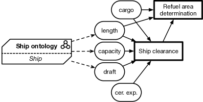
Figure 4: Graphical representation of an IDKB by extending the DMN notation for DRGs

4.2 Formalizing DKBs

From the formal point of view, the integration between a KB and a DRG is obtained by encoding the latter into $\mathsf{FOL}(\mathfrak{D})$, consequently enriching the KB with additional axioms that formally capture the decision logic. We provide the encoding in this section. Obviously, to encode a DRG we first need to encode the decisions contained therein. To this purpose, we build on the logic-based formalization of DMN introduced in [Calvanese et al. (2016)]. However, we cannot simply apply it as it is defined in [Calvanese et al. (2016)], since it does not follow the “object-oriented” approach required to interpret the application of a DRG in the presence of background knowledge. Specifically, that encoding formalizes decisions as formulae relating tuples of input values to tuples of output values, assuming no additional structure. In this work, we need to “objectify” the approach in [Calvanese et al. (2016)], considering decisions as axioms that predicate on the features of a certain object, and that in particular postulate that whenever certain (input) features satisfy given conditions, then the object must be connected to certain other values through corresponding (output) features. This approach is useful to handle the integration with background knowledge, but also to simply interpret the interconnection of multiple decisions into a DRG, making our object-oriented formalization of DMN decisions and DRGs is of independent interest.

Technically, we introduce an encoding $\tau$ that translates an IDKB $\overline{\mathfrak{X}}=\langle\Sigma,T,\mathfrak{G},C\rangle$ into a corresponding $\mathsf{FOL}(\mathfrak{D})$ IKB $\tau(\overline{\mathfrak{X}})$. The encoding can also be applied to a DKB, translating its intensional part as before while leaving its extensional part unaltered, i.e., given a DKB $\mathfrak{X}=\langle\Sigma,T,\mathfrak{G},C,A\rangle$ such that $\tau(\langle\Sigma,T,\mathfrak{G},C\rangle)=\langle\Sigma^{\prime},T^{\prime}\rangle$, we have $\tau(\mathfrak{X})=\langle\Sigma^{\prime},T^{\prime},A\rangle$. We next describe how $\Sigma^{\prime}$ and $T^{\prime}$ are actually constructed.

4.2.1 Encoding of the Signature

The signature corresponds to the original signature of $T$, augmented with a set of features that are obtained from the input data and the table attributes mentioned in $\mathfrak{G}$. To avoid potential name clashes coming from repeated attribute names in different decisions, each attribute corresponds to a feature whose name is obtained by concatenating the name of such an attribute with the name of its decision. Given a decision $\mathit{M}$ and an attribute $\mathbf{a}$ of $\mathit{M}$, we use notation $\mathit{M}\!\cdot\!\mathbf{a}$ to denote such a concatenated name. Formally, we get:

$$\Sigma^{\prime}=\Sigma\cup\{{P}/2\mid{P}\in\mathfrak{G}.I\}\cup\bigcup_{\mathit{M}\in\mathfrak{G}.\mathfrak{M}}\{\mathit{M}\!\cdot\!\mathbf{a}/2\mid\mathbf{a}\in\mathit{M}.I\cup\mathit{M}.I\}$$

Each so-generated feature has its first component typed with $\Delta$, and its second component typed with the datatype that is assigned by $\mathfrak{G}$ to its corresponding input data/attribute.

4.2.2 Encoding of the TBox

The TBox extends the original axioms in $T$ with additional axioms obtained by modularly encoding each decision and information flow of $\mathfrak{G}$:

$$T^{\prime}=T\cup\bigcup_{\mathit{M}\in\mathfrak{G}.\mathfrak{M}}\big{(}\tau_{C}(\mathit{M})\big{)}\cup\bigcup_{f\in\mathfrak{G}.\Rightarrow}\big{(}\tau(f)\big{)}$$

where the encoding $\tau_{C}(\mathit{M})$ of a decision table $\mathit{M}$ (parameterized by the bridge concept of $\mathfrak{X}$), and the encoding $\tau(f)$ of an information flow $f$, are detailed next.

Encoding of decisions. Let us consider the encoding $\tau_{C}(\mathit{M})$ of decision $\mathit{M}$, parameterized by bridge concept $C$. The encoding consists of the union of axioms obtained by translating: (i) the input/output attributes of $\mathit{M}$; (ii) the facet conditions or output ranges attached to such attributes; (iii) the rules in $\mathit{M}$ (considering also priorities and default outputs).

Encoding of attributes.  For each attribute $\mathbf{a}\in\mathit{M}.I\cup\mathit{M}.O$, the encoding $\tau_{C}$ produces two axioms: (i) a typing formula $\forall x,y.\mathit{M}\!\cdot\!\mathbf{a}(x,y)\rightarrow C(x)$, binding the domain of the attribute to the bridge concept; (ii) a functionality formula $\forall x,y,z.\mathit{M}\!\cdot\!\mathbf{a}(x,y)\land\mathit{M}\!\cdot\!\mathbf{a}(x,z)\rightarrow y=z$, declaring that every object of the bridge concept cannot be connected to more than one value through $\mathit{M}\!\cdot\!\mathbf{a}$. If $\mathbf{a}$ is an input attribute, functionality guarantees that the application of the decision table is unambiguous. If $\mathbf{a}$ is an output attribute, functionality simply captures that there is a single value present in an output cell of the decision. In general, multiple outputs for the same column may in fact be obtained when applying a decision but, if so, they would be still generated by different rules.

The exact same formalization does not only apply to the input attributes of a decision table, but also to the input data $\mathfrak{G}.I$ of the overall DRG $\mathfrak{G}$.

Example 6.

Consider the DKB in Example 5. The typing and functionality for the $\mathbf{Enter}$ input attribute for the refuel area determination decision (shown in Table 2, and for which we use compact name $\mathbf{Rad}$) are:

$$\forall x,y.\mathbf{Rad}\!\cdot\!\mathbf{Enter}(x,y)\rightarrow\textsl{Ship}(x)\qquad\forall x,y,z.\mathbf{Rad}\!\cdot\!\mathbf{Enter}(x,y)\land\mathbf{Rad}\!\cdot\!\mathbf{Enter}(x,z)\rightarrow y=z$$

 

Encoding of facet conditions and output ranges.  For each input attribute $\mathbf{a}\in\mathit{M}.I$, function $\tau_{C}$ produces a facet axiom imposing that the range of the feature must satisfy the restrictions imposed by the S-FEEL condition $\mathit{M}.\mathsf{InFacet}(\mathbf{a})$. In formulae:

$$\forall x,y.\mathit{M}\!\cdot\!\mathbf{a}(x,y)\rightarrow\tau^{y}(\mathit{M}.\mathsf{InFacet}(\mathbf{a})),$$

where, given an S-FEEL condition $\varphi$ and a variable $x$, function $\tau^{x}(\varphi)$ builds a unary $\mathsf{FOL}(\mathfrak{D})$ formula that encodes the application of $\varphi$ to $x$. This is defined as follows:

$$\tau^{x}(\varphi)\begin{cases}\mathit{true}&\text{if }\varphi=``\mathtt{-}"\\ x\neq\mathtt{v}&\text{if }\varphi=``\mathtt{not(}\mathtt{v}\mathtt{)}"\\ x=\mathtt{v}&\text{if }\varphi=``\mathtt{v}"\\ x\odot\mathtt{v}&\text{if }\varphi=``{\odot}\,\mathtt{v}"\text{ and }{\odot}\in\{{<},{>},{\leq},{\geq}\}\\ x>\mathtt{v}_{1}\land x<\mathtt{v}_{2}&\text{if }\varphi=``(\mathtt{v}_{1}..\mathtt{v}_{2})"\\ \ldots&\text{(similarly for the other types of intervals)}\\ \tau^{x}(\varphi_{1})\lor\tau^{x}(\varphi_{2})&\text{if }\varphi=``\varphi_{1}\mathtt{,}\varphi_{2}"\\ \end{cases}$$

The same mechanism is applied to the feature generated from each output attribute $\mathbf{b}\in\mathit{M}.O$, reinterpreting its output range $\mathsf{ORange}(\mathbf{b})=\langle\mathtt{v}_{1},\ldots,\mathtt{v}_{n}\rangle$ as the S-FEEL facet $``(\mathtt{v}_{1}\mathtt{,}\ldots\mathtt{,}\mathtt{v}_{n})"$. Also in this case, the exact same formalization does not only apply to the attributes of a decision table, but also to the input data $\mathfrak{G}.I$ of the overall DRG $\mathfrak{G}$.

Example 7.

Consider again the DKB in Example 5, and in particular the $\mathbf{length}$ attribute in Table 1 (for which we use the compact name $\mathbf{Sc}$). The facet $\mathsf{FOL}(\mathfrak{D})$ axioms for $\mathbf{length}$ is:

$$\forall x,y.\mathbf{Sc}\!\cdot\!\mathbf{length}(x,y)\rightarrow y\geq 0.$$

 

Encoding of rules.  Each rule is translated into an axiom expressing that, given an object:

if

the object has features for the input attributes of the rule whose values satisfy, attribute-wise, the S-FEEL conditions associated by the rule to such input attributes,

then

that object is also related, via output features, to the values associated by the rule to the output attributes.

Consider now a rule $r=\langle\mathsf{If},\mathsf{Then}\rangle$ in $\mathit{M}$. We first encode separately the input entry function $\mathsf{If}$ and the output entry function $\mathsf{Then}$. similarly to the case of single S-FEEL conditions, the encoding of $\mathsf{If}$ and $\mathsf{Then}$ is parameterized by a variable $x$, representing an object to which the input/output entries are applied. Formally, we thus get:

$$\tau^{x}(\mathsf{If})=\bigwedge_{\mathbf{a}\in\mathit{M}.I}\exists y.\Big{(}\mathit{M}\!\cdot\!\mathbf{a}(x,y)\land\tau^{y}(\mathsf{If}(\mathbf{a}))\Big{)}\qquad\tau^{x}(\mathsf{Then})=\bigwedge_{\mathbf{b}\in\mathit{M}.O}\exists y.\Big{(}\mathit{M}\!\cdot\!\mathbf{b}(x,y)\land\tau^{y}(\mathsf{Then}(\mathbf{b}))\Big{)}$$

where $\tau^{y}(\mathsf{If}(\mathbf{a}))$ applies the encoding for S-FEEL conditions defined before, on top of condition $\mathsf{If}(\mathbf{a})$ and using variable $y$, obtained from $x$ by navigating the feature corresponding to $\mathbf{a}$. The selection of $y$ obtained via existential quantification is unambiguous, as features are functional. A similar observation holds for $\tau^{y}(\mathsf{Then}(\mathbf{b}))$, noting that it simply produces a formula of the form $y=\mathtt{v}$, where $\mathtt{v}$ is the value assigned by rule $r$ to output attribute $\mathbf{b}$.

We now bind together the encoding of the rule premise and the rule conclusion into the overall encoding of rule $r$, which combines them into an implication formula. The body of this implication formula indicates when the rule trigger, which is partly based on the encoding of $r.\mathsf{If}$, and partly on the priority $\prec$ (cf. Section 3.2). Such a priority is in fact used to determine whether $r$ should really trigger on a given input object, or should instead stay quiescent because there is a higher-priority rule that triggers on the same object. With this notion at hand, we get:

$$\tau(r)=\forall x.\tau^{x}(r.\mathsf{If})\land\bigwedge_{r_{2}\in\mathit{M}.{R}\text{ and }r_{2}\prec r}\neg(\tau^{x}(r_{2}.\mathsf{If}))\rightarrow\tau^{x}(r.\mathsf{Then})$$

Due to the “prioritization formula” used in the last part of the body, the overall encoding of all rules in the DRG is at most quadratic in the number of rules. This priority-preserving encoding correctly captures the semantics of rules irrespectively of which single hit indicator is used in $\mathit{M}$, possibly introducing some unnecessary conjuncts:

• If $\mathit{M}$ semantically obeys to the unique hit strategy, then the input conditions of its rules are all mutually exclusive, and hence the prioritization formula is always trivially satisfied.

• If $\mathit{M}$ semantically obeys to the any hit strategy, then in case of multiple possible matches, all matching rules would actually return the same output values, and so the highest-priority matching rule can be safely selected.

• If $\mathit{M}$ adopts the priority hit policy, then the prioritization formula is actually needed to guarantee that the overall decision behaves according to what priority dictates.

Example 8.

Let us consider rule 2 in Table 1. Priority is, in this decision, irrelevant, as rules are indeed all non-overlapping. We can therefore ignore the prioritization formula, and simply get:

$$\begin{array}[]{@{}r@{}l@{}}\forall x.&\phantom{{}\land{}}(\exists e.\mathbf{Sc}\!\cdot\!\mathbf{cerExp}(x,e)\land e>\mathtt{today})\land(\exists l.\mathbf{Sc}\!\cdot\!\mathbf{length}(x,l)\land l<\mathtt{260})\\ &{}\land(\exists d.\mathbf{Sc}\!\cdot\!\mathbf{draft}(x,d)\land d<\mathtt{10})\land(\exists c.\mathbf{Sc}\!\cdot\!\mathbf{capacity}(x,c)\land c<\mathtt{1000})\rightarrow\exists o.\mathbf{Sc}\!\cdot\!\mathbf{enter}(x,o)\land o=\mathtt{y}.\end{array}$$

where $\textsl{enter}_{2}$ is obtained from output attribute $\mathbf{enter}$ in the context of Rule $2$.  

Since rules capture the intended input-output behavior of the decision, we have also to consider the case of default values for output attributes. Since default values are assigned when no rule triggers, we capture the “default output behavior” of decision $\mathit{M}$ as follows:

$$\forall x.\bigwedge_{r\in\mathit{M}.{R}}\neg(\tau^{x}(r.\mathsf{If}))\rightarrow\bigwedge_{\mathbf{b}\in\mathit{M}.O\text{ s.t.~{}}\mathit{M}.\mathsf{ODef}(\mathbf{b})\text{ is defined}}\Big{(}\exists y.\mathit{M}\!\cdot\!\mathbf{\mathbf{b}}(x,y)\land y=\mathit{M}.\mathsf{ODef}(\mathbf{b})\Big{)}$$

Note that it is not guaranteed that all attributes have a default value. If this is not the case, the formula above only binds those output facets whose corresponding attribute has a default value, leaving the other unspecified. This is perfectly compatible with the setting of DKBs, which indeed work under incomplete information.

Encoding of information flows. The encoding of information flows amounts to indicate that the source of an information flow feeds the target of the same information flow. This means that whenever a value is produced by the source, then this value is transferred into the target. Let $\langle P,\mathbf{a}\rangle$ be an information flow from input datum $P\in\mathfrak{G}.I$ to decision input attribute $\mathbf{a}\in\mathit{M}.I$ for some decision table $\mathit{M}\in\mathfrak{G}.\mathfrak{M}$, and let $\langle\mathbf{b},\mathbf{a}\rangle$ be an information flow from decision output attribute $\mathbf{b}\in\mathit{M}_{1}.O$ to decision input attribute $\mathbf{a}\in\mathit{M}_{2}.I$ for some $\mathit{M}_{1},\mathit{M}_{2}\in\mathfrak{G}.\mathfrak{M}$. Then, we get:

$$\tau(\langle P,\mathbf{a}\rangle)=\forall x,y.P(x,y)\rightarrow\mathit{M}\!\cdot\!\mathbf{\mathbf{a}}(x,y)\qquad\tau(\langle\mathbf{b},\mathbf{a}\rangle)=\forall x,y.\mathit{M}_{1}\!\cdot\!\mathbf{\mathbf{b}}(x,y)\rightarrow\mathit{M}_{2}\!\cdot\!\mathbf{\mathbf{a}}(x,y)$$

Example 9.

Consider the DRG of Figure 1(b), observing that the information requirement connecting the input datum length and the clearance decision is due to the underlying information flow between such an input datum and the $\mathbf{length}$ attribute of the ship clearance decision in Table 1. Such an information flow is captured by the formula:

$$\forall x,y.\textsl{length(x,y)}\rightarrow\mathbf{Sc}\!\cdot\!\mathbf{\mathbf{length}}(x,y)$$

 

4.3 Reasoning Tasks

We now formally revisit and extend the main reasoning tasks introduced by CDL16 DMN, considering here DKBs equipped with complex decisions captured in a DRG. In the following, we generically refer to all such reasoning tasks as DKB reasoning tasks.

By considering a single decision table inside the DRG, we focus on the compatibility of the decision with its policy hit, considering the semantics of its rules in the context of the overall DKB. At the level of the whole DRG, we instead focus on the input-output relationship induced by the DRG, arising from its internal decisions, information flows, and background knowledge. A related property is that of output coverage, which checks whether all mentioned output values of the DRG can possibly be produced. We also consider the two key properties of completeness and output determinability. Completeness of a DKB captures its ability of producing an overall output for the DRG for every configuration of values for its input data. Given a so-called template describing a set of objects, output determinability checks whether the template is informative enough to allow the DKB determining an overall output for the DRG given an object that instantiates the template. Recall that a DRG has some decision tables marked as outputs of the DRG. In this light, an output of the DRG consists of the combination of an output for each one of its output tables.

Compatibility with “unique hit”.  Unique hit is declared in a decision table $\mathit{M}$ by setting $\mathit{M}.H=\mathtt{u}$, and dictates that for every input object, at most one rule of $\mathit{M}$ triggers. To check whether this is indeed the case, we introduce the problem of compatibility with unique hit as:

Input:

IDKB $\overline{\mathfrak{X}}$, decision table $\mathit{M}\in\overline{\mathfrak{X}}.\mathfrak{G}.\mathfrak{M}$.

Question:

Is it the case that rules in $\mathit{M}.{R}$ do not overlap, i.e., never trigger on the same input? Formally:

$$\tau(\overline{\mathfrak{X}})\mathrel{\mathop{\models}\limits^{\vbox to0.0pt{\kern-2.0pt\hbox{$\scriptstyle?$}\vss}}}\bigwedge_{r_{1},r_{2}\in\mathit{M}.{R}\text{ s.t. }r_{1}\neq r_{2}}\neg\exists x.\Big{(}\tau^{x}(r_{1}.\mathsf{If})\land\tau^{x}(r_{2}.\mathsf{If})\Big{)}$$

Compatibility with “any hit”.  Any hit is declared in a decision table $\mathit{M}$ by setting $\mathit{M}.H=\mathtt{a}$, and postulates that whenever multiple rules may simultaneously trigger, they need to agree on the produced output. In this light, checking whether $\mathit{M}$ is compatible with this policy can be directly reduced to the case of unique hit, but considering only those pairs of rules in $\mathit{M}$ that differ in at least one output value.

Compatibility with “priority hit”.  Priority hit is declared in a decision table $\mathit{M}$ by setting $\mathit{M}.H=\mathtt{p}$, and postulates that whenever multiple rules may simultaneously trigger, the one with the highest priority is selected. This is directly incorporated in the formalization of rules, so rules are by design compatible with priority hit. However, selecting this policy may lead to the situation where a rule is masked by an higher-priority rule, and hence would never trigger [Calvanese et al. (2016)]. We thus consider that $\mathit{M}$ is compatible with the priority hit policy if none of its rules is masked. In this light, we introduce the problem of compatibility with priority hit as:

Input:

IDKB $\overline{\mathfrak{X}}$, decision table $\mathit{M}\in\overline{\mathfrak{X}}.\mathfrak{G}.\mathfrak{M}$.

Question:

Is it the case that no rule in $\mathit{M}.{R}$ is masked, i.e., there is at least one input object for which the rule triggers and no higher priority rule does? Formally:

$$\tau(\overline{\mathfrak{X}})\mathrel{\mathop{\models}\limits^{\vbox to0.0pt{\kern-2.0pt\hbox{$\scriptstyle?$}\vss}}}\bigwedge_{r_{1},r_{2}\in\mathit{M}.{R}\text{ s.t. }r_{1}\prec r_{2}}\exists x.\Big{(}\tau^{x}(r_{2}.\mathsf{If})\land\neg\tau^{x}(r_{1}.\mathsf{If})\Big{)}$$

I/O relationship.  A fundamental decision problem is to check whether the decision logic of a DKB induces a certain input/output relationship for a given object, in the presence of an ABox that captures additional extensional data about the domain of interest (such as values assigned to that object for the input attributes of the DKB). Specifically, the I/O relationship problem for a decision is defined as:

Input:

(i) DKB $\mathfrak{X}$, (ii) object $\mathtt{o}\in\Delta$, (iii) decision table $\mathit{M}\in\mathfrak{X}.\mathfrak{G}.\mathfrak{M}_{out}$, (iv) output attribute $\mathbf{b}\in\mathit{M}.O$, (v) value $\mathtt{v}\in\mathit{M}.\mathsf{AType}(\mathbf{b})$.

Question:

Is it the case that $\mathfrak{X}$ relates object $\mathtt{c}$ to value $\mathtt{v}$ via feature $\mathit{M}\!\cdot\!\mathbf{\mathbf{b}}$ ? Formally:

$$\tau(\mathfrak{X})\mathrel{\mathop{\models}\limits^{\vbox to0.0pt{\kern-2.0pt\hbox{$\scriptstyle?$}\vss}}}\mathit{M}\!\cdot\!\mathbf{\mathbf{b}}(\mathtt{o},\mathtt{v})$$

Output coverage.  Output coverage refers to the I/O relationship induced by an IDKB, in this case focusing on the possibility of actually deriving a specific value for one of the output attributes of the DRG contained in the IDKB. If this is not possible, then it means that, due to the interplay between different decision tables and their information flows, as well as the contribution of the background knowledge, some output configurations are never obtained. Specifically, we defined the output coverage problem as:

Input:

(i) IDKB $\overline{\mathfrak{X}}$, (ii) decision table $\mathit{M}\in\mathfrak{X}.\mathfrak{G}.\mathfrak{M}_{out}$, (iii) output attribute $\mathbf{b}\in\mathit{M}.O$, (iv) value $\mathtt{v}\in\mathit{M}.\mathsf{AType}(\mathbf{b})$.

Question:

Does $\overline{\mathfrak{X}}$ cover the possibility of outputting $\mathtt{v}$ for output attribute $\mathbf{b}$ of decision table $\mathit{M}$? Formally:

$$\tau(\overline{\mathfrak{X}})\mathrel{\mathop{\models}\limits^{\vbox to0.0pt{\kern-2.0pt\hbox{$\scriptstyle?$}\vss}}}\exists x,y.\mathit{M}\!\cdot\!\mathbf{b}(x,y)\land y=\mathtt{v}$$

Example 10.

Consider the IDKB $\overline{\mathfrak{X}}_{ship}$ of our running example, in particular as defined in Example 5. By focusing on the $\mathbf{RefuelArea}$ attribute of the output decision table refuel area determination (cf. 2), we can see that value $\mathtt{outdoor}$ is not covered by $\overline{\mathfrak{X}}_{ship}$. In fact, to produce such an output, rule $4$ should trigger, which in turn requires $\mathbf{length}$ and $\mathbf{cargo}$ to respectively be $>350$ and $>0.3$, and as well as $\mathbf{enter}$ to be $\mathtt{y}$. While the first two attributes are set by input data, the last is produced by the ship clearance table, which is defined on the same input data, plus further ones (cf. 1). However, the only rule of ship clearance that matches with the aforementioned conditions for $\mathbf{length}$ and $\mathbf{cargo}$, is in fact rule $9$, which however computes $\mathtt{n}$ for $\mathbf{enter}$, in turn falsifying the first condition of rule $4$ in refuel area determination. This formally confirms the informal discussion of Section 2.2. Notice that this issue does not depend on the background knowledge, but on the (partial) incompatibility between the two decision tables.  

Completeness.  Completeness asserts that the application of an IDKB to an arbitrary input object assigning values for the inputs of the DRG contained in the IDKB, is guaranteed to properly derive corresponding outputs. The DRG completeness problem is then defined as follows:

Input:

IDKB $\overline{\mathfrak{X}}$.

Question:

Is it the case that, for every object that assigns a value to each input of $\overline{\mathfrak{X}}.\mathfrak{G}.I$, $\overline{\mathfrak{X}}$ derives an output for each one of the output decision tables $\overline{\mathfrak{X}}.\mathfrak{G}.\mathfrak{M}_{out}$? Formally:

$$\tau(\overline{\mathfrak{X}})\mathrel{\mathop{\models}\limits^{\vbox to0.0pt{\kern-2.0pt\hbox{$\scriptstyle?$}\vss}}}\forall x.\Big{(}\bigwedge_{P\in\overline{\mathfrak{X}}.\mathfrak{G}.I}\exists y.P(x,y)\Big{)}\rightarrow\bigwedge_{\mathit{M}\in\overline{\mathfrak{X}}.\mathfrak{G}.\mathfrak{M}_{out}}\bigwedge_{\mathbf{b}\in\mathit{M}.O}\exists y.\mathit{M}\!\cdot\!\mathbf{b}(x,y)$$

Output determinability.  Output determinability is a refinement of completeness. It amounts at checking whether, given a template describing a set of objects (encoded as a unary $\mathsf{FOL}(\mathfrak{D})$ formula), that template description is detailed enough to ensure that the IDKB properly derives the outputs of its DRG for every object that belongs to the template. This is in fact the only decision problem that only makes sense in the presence of background knowledge. Specifically, the output determinability problem is defined as follows:

Input:

IDKB $\overline{\mathfrak{X}}$, unary $\mathsf{FOL}(\mathfrak{D})$ formula $\varphi(x)$ over signature $\overline{\mathfrak{X}}.\Sigma$ (called template).

Question:

Is it the case that, for every object that satisfies template $\varphi(x)$, $\overline{\mathfrak{X}}$ derives an output for each one of the output decision tables $\overline{\mathfrak{X}}.\mathfrak{G}.\mathfrak{M}_{out}$? Formally:

$$\tau(\overline{\mathfrak{X}})\mathrel{\mathop{\models}\limits^{\vbox to0.0pt{\kern-2.0pt\hbox{$\scriptstyle?$}\vss}}}\forall x.\varphi(x)\rightarrow\bigwedge_{\mathit{M}\in\overline{\mathfrak{X}}.\mathfrak{G}.\mathfrak{M}_{out}}\bigwedge_{\mathbf{b}\in\mathit{M}.O}\exists y.\mathit{M}\!\cdot\!\mathbf{b}(x,y)$$

It is easy to see that completeness is a special case of output determinability, where the template simply describes objects that have all input data attached to them: $\varphi(x)=\bigwedge_{P\in\overline{\mathfrak{X}}.\mathfrak{G}.I}\exists y.P(x,y)$.

Example 11.

Consider again the IDKB $\overline{\mathfrak{X}}_{ship}$ of Example 5. We have already discussed in Section 2.2 that to properly apply the decision logic formalized in $\overline{\mathfrak{X}}_{ship}$, it is sufficient to know its type, cargo residuals, and certificate expiration date. This can be formalized as an output determinability problem, using as template the unary formula:

$$\varphi_{ship}(x)=\exists e,c,t.\textsl{cerExp}(x,e)\land\textsl{capacity}(x,c)\land\textsl{stype}(x,t)$$

 

DMN reasoning tasks.  We stress that, with the exception of output determinacy, all the decision problems identified here are relevant also when background knowledge is not present, and consequently a given DRG is interpreted under the assumption of complete information. In this case, compatibility with the different hit indicators, output coverage, and completeness, can all be captured as explained above, by simply setting $T=\emptyset$. To account for I/O relationship, we have to put $T=\emptyset$, and fix $A$ to contain exactly the following facts: (i) a fact $C(\mathtt{o})$ for the selected object $\mathtt{o}$; (ii) a set of facts of the form $\{P(\mathtt{o},\mathtt{v}_{j})\mid P\in\mathfrak{X}.\mathfrak{G}.I\}$, denoting the assignment of input attributes for $\mathtt{o}$ to the corresponding values of interest, one per input data of the DRG. In addition, all the identified decision problems can also be studied in the case of a single decision table $\mathit{M}$, not immersed inside a DRG. This requires to construct the trivial DRG $\mathfrak{G}_{\mathit{M}}$ that contains $\mathit{M}$ as the only decision table, marks it also as output table, and contains input data that exactly match (and feed via information flows) the input attributes of $\mathit{M}$. Properties of $\mathit{M}$ in the presence of background knowledge can then be assessed by studying a DKB or IDKB that uses $\mathfrak{G}_{\mathit{M}}$ as DRG.

5 Reasoning on Decision Knowledge Bases

While the translation from DKBs to $\mathsf{FOL}(\mathfrak{D})$ presented in Section 4.2 provides a logic-based semantics for DKBs, it does not give any insight on how to actually approach the different decision problems of Section 4.3. In fact, none of such problems can be solved in the general case of full $\mathsf{FOL}(\mathfrak{D})$. Specifically, decidability and complexity of such reasoning tasks depend on the background knowledge and on the decision component. Since the decision component comes with the fixed S-FEEL language and DRG structure, we approach this problem as follows. First, we show that DMN decision tables written in S-FEEL, and interconnected in a DRG, can be encoded in $\mathsf{ALCH}(\mathfrak{D})$. Then, we show that all reasoning tasks defined in Section 4.3 can be reduced to (un)satisfiability of an $\mathsf{ALCH}(\mathfrak{D})$ concept w.r.t. a KB consisting of the union of the background knowledge with the $\mathsf{ALCH}(\mathfrak{D})$ formalization of the DRG. This implies that all such reasoning tasks can be carried out in ExpTime, if the background knowledge is expressed in $\mathsf{ALCH}(\mathfrak{D})$.

5.1 Encoding DRGs in $\mathsf{ALCH}(\mathfrak{D})$

We revisit the translation from DKBs to $\mathsf{FOL}(\mathfrak{D})$ introduced in 4.2, showing that the translation of DRGs can be reconstructed so as to obtain an $\mathsf{ALCH}(\mathfrak{D})$ IKB.

Given a bridge concept $C$ and a DRG $\mathfrak{G}$, we introduce a translation function $\rho_{C}$ that encodes $\mathit{M}$ into the corresponding $\mathsf{ALCH}(\mathfrak{D})$ IKB $\rho_{C}(\mathfrak{G})=\langle\Sigma_{\mathfrak{G}},T_{\mathfrak{G}}\rangle$, using $C$ to provide a context for the encoding. The signature is obtained as in Section 4.2.1. The encoding of $T_{\mathfrak{G}}$ reconstructs that of Section 4.2, and in fact deals with input data and information flows of the $\mathfrak{G}$, as well as input/output attributes, facets, and rules of decision tables $\mathfrak{G}.\mathfrak{M}$.

Encoding of attributes and input data.  For each decision table $\mathit{M}\in\mathfrak{G}.\mathfrak{M}$, and each attribute $\mathbf{a}\in\mathit{M}.I\cup\mathit{M}.O$, encoding $\rho_{C}$ produces the typing axiom $\exists\mathit{M}\!\cdot\!\mathbf{a}\sqsubseteq C$. The same holds for all input data $\mathfrak{G}.I$. Functionality is not explicitly asserted, since $\mathsf{ALCH}(\mathfrak{D})$ features are functional by default.

Encoding of facet conditions.  For each decision table $\mathit{M}\in\mathfrak{G}.\mathfrak{M}$, and each input attribute $\mathbf{a}\in\mathit{M}.I$, encoding $\rho_{C}$ produces a derived datatype declaration of the form

$$\exists\mathit{M}\!\cdot\!\mathbf{a}\sqsubseteq\rho^{\mathit{M}\!\cdot\!\mathbf{a},\mathsf{AType}(\mathbf{a})}(\mathit{M}.\mathsf{InFacet}(\mathbf{a}))$$

where, given an S-FEEL condition $\varphi$, a facet $P$, and a datatype $type$, function $\rho^{P,type}$ produces an $\mathsf{ALCH}(\mathfrak{D})$ concept capturing objects that have an outgoing facet of type $P$, whose range satisfies $\varphi$. This is defined as follows:

$$\rho^{P,type}(\varphi)=\begin{cases}\top&\text{if }\varphi=``\mathtt{-}"\\ \neg\exists P.type[=_{\mathtt{v}}]&\text{if }\varphi=``\mathtt{not(}\mathtt{v}\mathtt{)}"\\ \exists P.type[=_{\mathtt{v}}]&\text{if }\varphi=``\mathtt{v}"\\ \exists P.type[\odot_{\mathtt{v}}]&\text{if }\varphi=``\odot\mathtt{v}"\text{ and }\odot\in\{<,>,\leq,\geq\}\\ \exists P.type[>_{\mathtt{v}_{1}}\land<_{\mathtt{v}_{2}}]&\text{if }\varphi=``(\mathtt{v}_{1}..\mathtt{v}_{2})"\\ \ldots&\text{(similarly for the other types of intervals)}\\ \rho^{P,type}(\varphi_{1})\sqcup\rho^{P,type}(\varphi_{2})&\text{if }\varphi=``\varphi_{1}\mathtt{,}\varphi_{2}"\\ \end{cases}$$

The same encoding is applied by $\rho_{C}$ to each input data $P\in\mathfrak{G}.I$ with its facet $\mathfrak{G}.\mathsf{InFacet}(P)$, and, for every decision table $\mathit{M}\in\mathfrak{G}.\mathfrak{M}$, to each output attribute $\mathbf{b}\in\mathit{M}.O$ with its range $\mathit{M}.\mathsf{ORange}(\mathbf{b})$.

Example 12.

Consider the $\mathbf{length}$ attribute of the ship clearance decision table (cf. Table 1). With Ship as bridge concept, the typing and facet $\mathsf{ALCH}(\mathfrak{D})$ formulae for $\mathbf{length}$ are:

$$\exists\textsl{length}\sqsubseteq\textsl{Ship}\qquad\exists\textsl{length}\sqsubseteq\exists\textsl{length.real}[>_{0}]$$

 

Encoding of rules. Consider a decision table $\mathit{M}$, and one of its rules $r=\langle\mathsf{If},\mathsf{Then}\rangle$. The encoding of $\mathsf{If}$ (resp., $\mathsf{Then}$) constructs an $\mathsf{ALCH}(\mathfrak{D})$ concept that has all features mentioned by the input (resp., output) attributes, restricted so as to satisfy the corresponding input condition (resp., output value) imposed by $\mathsf{If}$ (resp., $\mathsf{Then}$):

$$\rho_{C}(\mathsf{If})=\bigsqcap_{\mathbf{a}\in\mathit{M}.I}\rho^{\mathit{M}\!\cdot\!\mathbf{a},\mathit{M}.\mathsf{AType}(\mathbf{a})}(\mathsf{If}(\mathbf{a}))\qquad\rho_{C}(\mathsf{Then})=\bigsqcap_{\mathbf{b}\in\mathit{M}.O}\rho^{\mathit{M}\!\cdot\!\mathbf{b},\mathit{M}.\mathsf{AType}(\mathbf{b})}(\mathsf{If}(\mathbf{b}))$$

We combine these two encodings into a global encoding of rule $r$, imposing that the rule indeed triggers only if no higher-priority rule triggers:

$$\rho_{C}(r)=\rho_{C}(r.\mathsf{If})\sqcap\bigsqcap_{r_{2}\in\mathit{M}.{R}\text{ and }r_{2}\prec r}\neg\rho_{C}(r_{2}.\mathsf{If})\sqsubseteq\rho_{C}(r.\mathsf{Then})$$

Example 13.

Consider the ship clearance decision table, referred by name $\mathbf{Sc}$. In particular, consider rule 2 of this decision table, as shown Table 1. By assuming that this is the top-priority rule, it is encoded in $\mathsf{ALCH}(\mathfrak{D})$ as:

$$\begin{array}[]{@{}l}\exists\mathbf{Sc}\!\cdot\!\mathbf{cerExp}.\textsl{real}[>_{\mathtt{today}}]\and\exists\mathbf{Sc}\!\cdot\!\mathbf{length}.\textsl{real}[<_{\mathtt{260}}]\\ {}\and\exists\mathbf{Sc}\!\cdot\!\mathbf{draft}.\textsl{real}[<_{\mathtt{10}}]\and\exists\mathbf{Sc}\!\cdot\!\mathbf{cap}.\textsl{real}[<_{\mathtt{1000}}]~{}\sqsubseteq~{}\exists\mathbf{Sc}\!\cdot\!\mathbf{enter}.\textsl{string}[=_{\mathtt{Y}}]\end{array}$$

 

We also have to handle the generation of default values, when no rule in $\mathit{M}$ triggers. This is captured by the following, additional axiom:

$$\bigsqcap_{r\in\mathit{M}.{R}}\neg\rho_{C}(r.\mathsf{If})~{}\sqsubseteq~{}\bigsqcap_{\mathbf{b}\in\mathit{M}.O\text{ s.t.~{}}\mathit{M}.\mathsf{ODef}(\mathbf{b})\text{ is defined}}\Big{(}\exists\mathit{M}\!\cdot\!\mathbf{\mathbf{b}}[=_{\mathit{M}.\mathsf{ODef}(\mathbf{b})}]\Big{)}$$

Encoding of information flows. Let $\langle P,\mathbf{a}\rangle$ be an information flow from input datum $P\in\mathfrak{G}.I$ to decision input attribute $\mathbf{a}\in\mathit{M}.I$ for some decision table $\mathit{M}\in\mathfrak{G}.\mathfrak{M}$, and let $\langle\mathbf{b},\mathbf{a}\rangle$ be an information flow from decision output attribute $\mathbf{b}\in\mathit{M}_{1}.O$ to decision input attribute $\mathbf{a}\in\mathit{M}_{2}.I$ for some $\mathit{M}_{1},\mathit{M}_{2}\in\mathfrak{G}.\mathfrak{M}$. Their $\mathsf{ALCH}(\mathfrak{D})$ encoding consists of the following facet inclusion assertions:

$$\rho_{C}(\langle P,\mathbf{a}\rangle)=P~{}\sqsubseteq\mathit{M}\!\cdot\!\mathbf{\mathbf{a}}\qquad\rho_{C}(\langle\mathbf{b},\mathbf{a}\rangle)=\mathit{M}_{1}\!\cdot\!\mathbf{\mathbf{b}}~{}\sqsubseteq\mathit{M}_{2}\!\cdot\!\mathbf{\mathbf{a}}$$

Correctness of the encoding. Thanks to the fact that $\mathsf{ALCH}(\mathfrak{D})$ can be seen as a well-behaved fragment of $\mathsf{FOL}(\mathfrak{D})$, we can directly establish that the $\mathsf{ALCH}(\mathfrak{D})$ encoding of DRGs properly reconstructs the original $\mathsf{FOL}(\mathfrak{D})$ encoding.

Theorem 2.

For every DRG $\mathfrak{G}$, and every (bridge) concept $C$, we have that the $\mathsf{FOL}(\mathfrak{D})$ IKB $\tau_{C}(\mathfrak{G})$ is logically equivalent to the $\mathsf{ALCH}(\mathfrak{D})$ IKB $\rho_{C}(\mathfrak{G})$.

Proof.

Direct by definition of the encodings $\tau_{C}$ and $\rho_{C}$, noting that, once $\mathsf{ALCH}(\mathfrak{D})$ IKB $\rho_{C}(\mathit{M})$ is represented in $\mathsf{FOL}(\mathfrak{D})$ using the standard $\mathsf{FOL}(\mathfrak{D})$ encoding of $\mathsf{ALCH}(\mathfrak{D})$, it becomes identical to the $\mathsf{FOL}(\mathfrak{D})$ IKB $\tau_{C}(\mathit{M})$.

5.2 Reasoning over $\mathsf{ALCH}(\mathfrak{D})$ Decision Knowledge Bases

By exploiting the $\mathsf{ALCH}(\mathfrak{D})$ encoding of a DRG, we have now the possibility of studying if and how the different reasoning tasks introduced in Section 4.3 can be effectively carried out in the case where the background knowledge is also represented as an $\mathsf{ALCH}(\mathfrak{D})$ (I)KB.

We say that an IDKB $\overline{\mathfrak{X}}$ is an $\mathsf{ALCH}(\mathfrak{D})$ IDKB if its TBox $\mathfrak{X}.T$ is an $\mathsf{ALCH}(\mathfrak{D})$ TBox. As for a $DKB$ $\mathfrak{X}$, we require the same, and also that and its ABox $\mathfrak{X}.A$ is an $\mathsf{ALCH}(\mathfrak{D})$ ABox. Given an $\mathsf{ALCH}(\mathfrak{D})$ DKB $\mathfrak{X}$, we extend the encoding function $\rho_{\mathfrak{X}.C}$ introduced in Section 5.1 so as to make it applicable over the entire DKB, as follows: $\rho_{C}(\mathfrak{X})=\langle\mathfrak{X}.\Sigma\cup\Sigma^{\prime},\mathfrak{X}.T\cup T^{\prime},\mathfrak{X}.A\rangle$, where $\langle\Sigma^{\prime},T^{\prime}\rangle=\rho_{C}(\mathfrak{X}.\mathfrak{G})$ (similarly for an $\mathsf{ALCH}(\mathfrak{D})$ IKB). With these notions at hand, we show the following.

Theorem 3.

In the case of $\mathsf{ALCH}(\mathfrak{D})$ DKBs, all DKB reasoning tasks can be reduced to standard $\mathsf{ALCH}(\mathfrak{D})$ reasoning tasks.

Proof.

We show, for each DKB reasoning task, how it can be reduced to a polynomial number of $\mathsf{ALCH}(\mathfrak{D})$ concept (un)satisfiability or instance checking tests w.r.t. an $\mathsf{ALCH}(\mathfrak{D})$ KB.

Compatibility with “unique hit”.  We use the following algorithm, relying on $\mathsf{ALCH}(\mathfrak{D})$ satisfiability checking. In the following algorithm, the usage of $\prec$ is not needed for correctness, but actually matters to reduce the number of checks (being the notion of overlap symmetric).

⬇

1boolean compatibleWithU(IDKB $\overline{\mathfrak{X}}$, Table $\mathit{M}\in\overline{\mathfrak{X}}.\mathfrak{M}$) {

2 for each $r_{1},r_{2}\in\mathit{M}.{R}$ such that $r_{1}\prec r_{2}$ {

3 if $\rho_{\overline{\mathfrak{X}}.C}(r_{1}.\mathsf{If})\sqcap\rho_{\overline{\mathfrak{X}}.C}(r_{2}.\mathsf{If})$ is satisfiable w.r.t. $\rho_{\overline{\mathfrak{X}}.C}(\overline{\mathfrak{X}})$

4 return false;

5 }

6 return true;

7}

Compatibility with “any hit”.  We use exactly the same algorithm used for compatibility with “unique hit”, with the only difference that in line 2 we add $r_{1}.\mathsf{Then}=r_{2}.\mathsf{Then}$ as a further condition, to ensure that the output values produced by $r_{1}$ and $r_{2}$ coincide.

Compatibility with “priority hit”.  We use the following algorithm, relying on $\mathsf{ALCH}(\mathfrak{D})$ unsatisfiability checking.

⬇

1boolean compatibleWithP(IDKB $\overline{\mathfrak{X}}$, Table $\mathit{M}\in\overline{\mathfrak{X}}.\mathfrak{M}$) {

2 for each $r_{1},r_{2}\in\mathit{M}.{R}$ such that $r_{1}\prec r_{2}$ {

3 if $\neg\rho_{\overline{\mathfrak{X}}.C}(r_{1}.\mathsf{If})\sqcap\rho_{\overline{\mathfrak{X}}.C}(r_{2}.\mathsf{If})$ is unsatisfiable w.r.t. $\rho_{\overline{\mathfrak{X}}.C}(\overline{\mathfrak{X}})$

4 return false;

5 }

6 return true;

7}

I/O relationship.  We use the following algorithm, relying on $\mathsf{ALCH}(\mathfrak{D})$ instance checking.

⬇

1boolean IORelationship(DKB $\mathfrak{X}$, Table $\mathit{M}\in\overline{\mathfrak{X}}.\mathfrak{M}_{out}$, Object $\mathtt{o}\in\Delta$,

2 Attribute $\mathbf{b}\in\mathit{M}.O$, Value $\mathtt{v}\in\mathit{M}.\mathsf{AType}(\mathbf{b})$) {

3 return $\langle\mathtt{o},\mathtt{v}\rangle$ instance of $\mathit{M}\!\cdot\!\mathbf{\mathbf{b}}$ w.r.t. $\rho_{\mathfrak{X}.C}(\mathfrak{X})$;

4}

Output coverage.  We use the following algorithm, relying on $\mathsf{ALCH}(\mathfrak{D})$ satisfiability checking.

⬇

1boolean CoversOutput(IDKB $\overline{\mathfrak{X}}$, Table $\mathit{M}\in\overline{\mathfrak{X}}.\mathfrak{M}_{out}$,

2 Attribute $\mathbf{b}\in\mathit{M}.O$, Value $\mathtt{v}\in\mathit{M}.\mathsf{AType}(\mathbf{b})$) {

3 return $\exists\mathit{M}\!\cdot\!\mathbf{\mathbf{b}}[=_{\mathtt{v}}]$ is satisfiable w.r.t. $\rho_{\overline{\mathfrak{X}}.C}(\overline{\mathfrak{X}})$;

4}

Completeness. We use the following algorithm, relying on $\mathsf{ALCH}(\mathfrak{D})$ satisfiability checking.

⬇

1boolean Complete(IDKB $\overline{\mathfrak{X}}$) {

2 for each $\mathit{M}\in\overline{\mathfrak{X}}.\mathfrak{G}.\mathfrak{M}_{out}$ {

3 for each $\mathbf{b}\in\mathit{M}.O$ {

4 if $\bigsqcap_{P\in\overline{\mathfrak{X}}.\mathfrak{G}.I}\exists P\sqcap\neg\exists\mathit{M}\!\cdot\!\mathbf{b}$ is satisfiable w.r.t. $\rho_{\overline{\mathfrak{X}}.C}(\overline{\mathfrak{X}})$

5 return false;

6 }

7 }

8 return true;

9}

Output determinability. We use the following algorithm, relying on $\mathsf{ALCH}(\mathfrak{D})$ satisfiability checking. Obviously, we consider templates described by $\mathsf{ALCH}(\mathfrak{D})$ concepts.

⬇

1boolean DeterminesOutput(IDKB $\overline{\mathfrak{X}}$, $\mathsf{ALCH}(\mathfrak{D})$ Concept $\Phi$) {

2 for each $\mathit{M}\in\overline{\mathfrak{X}}.\mathfrak{G}.\mathfrak{M}_{out}$ {

3 for each $\mathbf{b}\in\mathit{M}.O$ {

4 if $\Phi\sqcap\neg\exists\mathit{M}\!\cdot\!\mathbf{b}$ is satisfiable w.r.t. $\rho_{\overline{\mathfrak{X}}.C}(\overline{\mathfrak{X}})$

5 return false;

6 }

7 }

8 return true;

9}

It is straightforward to check that all the presented algorithms correctly reconstruct the corresponding $\mathsf{FOL}(\mathfrak{D})$ decision problems.

Example 14.

As discussed in Example 2, the ship ontology in Table 1(c) can be formalized in $\mathsf{ALCH}(\mathfrak{D})$. Hence, the maritime security DKB of Example 5 is actually an $\mathsf{ALCH}(\mathfrak{D})$ DKB. Thanks to Theorem 3, standard $\mathsf{ALCH}(\mathfrak{D})$ reasoning tasks can then be used to carry out all the introduced reasoning tasks over such a DKB.  

Thanks to Theorems 1 and 3, we obtain two additional key results. The first result characterizes the complexity of $DKB$ reasoning in the case of $\mathsf{ALCH}(\mathfrak{D})$ DKBs.

Corollary 1.

All DKB reasoning tasks over $\mathsf{ALCH}(\mathfrak{D})$ DKBs can be decided in ExpTime.

Notice that the complexity of reasoning in DKBs that employ different ontology languages to capture the background knowledge, depends on the actual ontology language of choice, considering that the encoding of DRGs brings an $\mathsf{ALCH}(\mathfrak{D})$ component. In general, since $\mathsf{ALCH}(\mathfrak{D})$ datatypes come with unary predicates, our approach naturally lends itself to be combined with OWL 2 ontologies, and the $\mathsf{ALCH}(\mathfrak{D})$ encoding of DRGs can in fact be directly represented in OWL 2.

Corollary 2.

All DKB reasoning tasks over $\mathsf{ALCH}(\mathfrak{D})$ DKBs can be tackled by standard OWL 2 reasoners.

This is an important observation, since one can then resort to state-of-the-art reasoners for OWL 2 that have been developed and optimized over the years [Tsarkov and Horrocks (2006), Sirin and Parsia (2006), Shearer et al. (2008)]. When considering reasoning tasks that only focus on intensional knowledge, that is, all reasoning tasks introduced in Section 4.3 with the exception of I/O relationship, it is also possible to rely on reasoners for OWL 2 TBoxes that do not support datatypes. In fact, we can reconstruct the technique introduced by [Theorem 2.14]Lutz02c to encode away unary concrete domains, so as to compile away datatypes from IDKBs, finally obtaining a pure $\mathsf{ALCH}$ TBox. However, this requires to exhaustively apply datatype reasoning during the compilation process, Hence, it remains open whether this introduces an effective improvement over full OWL 2 reasoners, which typically apply datatype reasoning lazily, only when needed.

A second open problem is to show whether DRGs can be encoded in weaker ontology languages, so as to obtain more refined complexity bounds for the different DKB reasoning tasks. The main difficulty here stems from the fact that extensions of lightweight DLs with datatypes have been so far much less investigated than their corresponding expressive counterparts. In particular, currently known lightweight DLs with datatypes are equipped with an ontology language that is too weak to encode DRGs [Artale et al. (2012), Savkovic and Calvanese (2012)].

6 Related Work

To the best of our knowledge, this work is the first approach that combines DMN DRGs with background knowledge, building on the preliminary results obtained in [Calvanese et al. (2017)] for the case of single decision tables. In addition, it is also the first approach that considers reasoning tasks over DMN DRGs, even without considering the contribution of background knowledge. In this light, it can be considered as a natural extension of the formalization effort carried out in [Calvanese et al. (2016)].

Reasoning on single decision tables has instead attracted a lot of interest in the literature, an interest recently revived by the introduction of the DMN standard. In particular, reasoning tasks that aim at assessing completeness, consistency and redundancy of decision tables, are widely recognized [CODASYL Decision Table Task Group (1982)]. The literature flourishes of ad-hoc, algorithmic techniques to account for such decision problems, considering specific datatypes. In particular, one long-standing line of research comprises techniques to reason about decision tables whose attributes are either boolean or enumerative (i.e., categorical) [Pawlak (1987), Hoover and Chen (1995), Zaidi and Levis (1997)]. Some of these techniques have been actually implemented inside well-known tools like Prologa [Vanthienen and Dries (1994), Vanthienen et al. (1998)].

The main drawback of these approaches is that they do not directly account for numerical datatypes: in the presence of conditions expressing numerical intervals, they require to restructure their corresponding rules so as to ensure that all intervals are disjoint. [Calvanese et al. (2016)] introduces ad-hoc algorithmic techniques based on a geometric interpretation of rules, and shows that such techniques outperform previous approaches, while being able to naturally handle numerical domains. The DMN component of Signavio detects overlapping and missing rules by natively dealing with numerical data types. However, the actual algorithms used to conduct such checks have not been disclosed. OpenRules builds instead on constraint satisfaction techniques to analyze rules containing numerical attributes.

Differently from all these approaches, we consider here full DMN DRGs in the presence of background knowledge. This richer setting also demands a wider and more sophisticated set of reasoning tasks, going beyond completeness and consistency of single decision tables. For such advanced reasoning tasks, we do not develop ad-hoc algorithmic techniques, but instead rely on a fully automated encoding of the input specification, and of the tasks of interest, into standard reasoning tasks for the DL $\mathsf{ALCH}(\mathfrak{D})$. Efficient, state-of-the-art reasoners have been devised for expressive DLs, such as OWL 2 [Horrocks et al. (2006), Bao et al. (2012)], that fully capture $\mathsf{ALCH}(\mathfrak{D})$ [Tsarkov and Horrocks (2006), Sirin and Parsia (2006), Shearer et al. (2008)], setting the baseline for a future experimental evaluation of the techniques presented in this paper, considering real and synthetic data. In addition, by inspecting the proof of Theorem 3, it is easy to see that all the presented algorithms can be easily modified so as to return the actual, involved rules whenever a property is not satisfied.

From the knowledge representation point of view, this work touches the widely studied, and still debated, problem of integrating rules and ontologies. This problem has been approached in different ways, depending on the expressiveness of the rule and of the ontology languages [Drabent et al. (2009), Krisnadhi et al. (2011)]. On the one hand, several proposals have been devised to integrate rules and ontologies by defining suitable “hybrid” semantics [Motik and Rosati (2010)], or by considering rules accessing ontologies as an external knowledge component [Eiter et al. (2017)]. On the other hand, “controlled” forms of rules have been integrated with ontologies by reformulating them as additional ontological axioms [Krisnadhi et al. (2011)]. Our contribution belongs to the latter family, thanks to the interesting trade-off between expressiveness and simplicity offered by the DMN S-FEEL language.

7 Conclusions

In this work, we have provided a threefold contribution to the area of decision management, recently revived by the introduction of the DMN OMG standard. First, we have introduced decision knowledge bases (DKBs) as a conceptual framework to integrate DMN complex decisions with background knowledge, expressed as a description logic (DL) knowledge base. On top of this conceptual framework, we have then introduced key reasoning tasks to ascertain the correctness of a DKB. Second, we have provided a logic-based formalization of DKBs and their corresponding reasoning tasks, using multi-sorted FOL equipped with datatypes. Third, we have focused our attention on the interesting case where the background knowledge is expressed using $\mathsf{ALCH}(\mathfrak{D})$, an extension of the well-known description logic $\mathsf{ALC}$ with multiple datatypes, and a sublanguage of the standard ontology language OWL 2. In this setting, we have shown that all the aforementioned reasoning tasks are decidable in ExpTime, and lend themselves to be carried out using standard reasoners for expressive description logics. On the way of proving this result, we have shown that TBox and ABox reasoning for $\mathsf{ALCH}$ extended with multiple datatypes stays within ExpTime, which is of independent interest.

These three contributions pave the ways towards a concrete implementation of the presented framework and techniques. We plan to realize this implementation and to consequently carry out an experimental evaluation by considering not only full DKBs, but also DKBs consisting of a single decision table, as well as complex decisions without background knowledge, so as to better identify the sources of complexity, and to see how well a general approach of this form compares with the ad-hoc algorithms developed in the literature. In spite of the ExpTime upper bound for reasoning on DKBs, we believe that an effective, scalable implementation is actually at reach, thanks to the availability of solid, optimized reasoners for OWL 2.

In addition to the implementation effort, we are interested in refining our complexity analysis, in particular aiming at tighter bounds on the complexity caused by the decision component. Specifically, we plan to systematically study how lightweight DLs equipped with datatypes [Savkovic and Calvanese (2012), Artale et al. (2012)], for which currently the ontology language is too weak to capture complex DMN decision tables, can be extended, focusing on their ability of dealing with datatypes and features. We would like to single out more precisely the complexity brought in by a DMN complex decision table, with the aim of capturing more complex forms of tables, without compromising the low computational complexity of reasoning in lightweight DLs (AC⁰ in the size of the data). As a consequence, this would pave the way towards lightweight DKBs.

Acknowledgements. 

This research is partly supported by the Estonian Research Council Grant IUT20-55, by the project “Reasoning and Enactment for Knowledge-Aware Processes” (REKAP), which is funded through the 2017 call issued by the Research Committee of the Free University of Bozen-Bolzano, and by the Euregio Interregional Project Network IPN12 “Knowledge-Aware Operational Support” (KAOS), which is funded by the “European Region Tyrol-South Tyrol-Trentino” (EGTC) under the first call for basic research projects and by the Free University of Bozen-Bolzano.

References

- Artale et al. (2012) Artale, A., Kontchakov, R., and Ryzhikov, V. 2012. DL-Lite with attributes and datatypes. In Proc. of the 20th Eur. Conf. on Artificial Intelligence (ECAI). Frontiers in Artificial Intelligence and Applications, vol. 242. IOS Press, 61–66.
- Baader et al. (2007) Baader, F., Calvanese, D., McGuinness, D., Nardi, D., and Patel-Schneider, P. F., Eds. 2007. The Description Logic Handbook: Theory, Implementation and Applications, 2nd ed. Cambridge University Press.
- Baader and Sattler (2000) Baader, F. and Sattler, U. 2000. Tableau algorithms for description logics. In Proc. of the 9th Int. Conf. on Automated Reasoning with Analytic Tableaux and Related Methods (TABLEAUX). Lecture Notes in Artificial Intelligence, vol. 1847. Springer, 1–18.
- Bao et al. (2012) Bao, J. et al. 2012. OWL 2 Web Ontology Language document overview (second edition). W3C Recommendation, World Wide Web Consortium. Dec. Available at http://www.w3.org/TR/owl2-overview/.
- Batoulis et al. (2015) Batoulis, K., Meyer, A., Bazhenova, E., Decker, G., and Weske, M. 2015. Extracting decision logic from process models. In Proc. of the 27th Int. Conf. on Advanced Information Systems Engineering (CAiSE). Springer.
- Calvanese et al. (2016) Calvanese, D., Dumas, M., Laurson, Ü., Maggi, F. M., Montali, M., and Teinemaa, I. 2016. Semantics and analysis of DMN decision tables. In Proc. of the 14th Int. Conf. on Business Process Management (BPM). Lecture Notes in Computer Science, vol. 9850. Springer, 217–233.
- Calvanese et al. (2017) Calvanese, D., Dumas, M., Maggi, F. M., and Montali, M. 2017. Semantic DMN: Formalizing decision models with domain knowledge. In Proc. of the 1st Int. Joint Conf. on Rules and Reasoning (RuleML+RR). Lecture Notes in Computer Science, vol. 10364. Springer, 70–86.
- CODASYL Decision Table Task Group (1982) CODASYL Decision Table Task Group. 1982. A Modern Appraisal of Decision Tables: a CODASYL Report. ACM.
- Drabent et al. (2009) Drabent, W., Eiter, T., Ianni, G., Krennwallner, T., Lukasiewicz, T., and Maluszynski, J. 2009. Hybrid reasoning with rules and ontologies. In Semantic Techniques for the Web, The REWERSE Perspective, F. Bry and J. Maluszynski, Eds. Lecture Notes in Computer Science, vol. 5500. Springer, 1–49.
- Eiter et al. (2017) Eiter, T., Kaminski, T., Redl, C., Schüller, P., and Weinzierl, A. 2017. Answer set programming with external source access. In Reasoning Web: Semantic Interoperability on the Web – 13th Int. Summer School Tutorial Lectures (RW). Lecture Notes in Computer Science, vol. 10370. Springer, 204–275.
- Eiter et al. (2009) Eiter, T., Lutz, C., Ortiz, M., and Simkus, M. 2009. Query answering in description logics: The Knots approach. In Proc. of the 16th Int. Workshop on Logic, Language, Information and Computation (WoLLIC). Lecture Notes in Computer Science, vol. 5514. Springer, 26–36.
- Enderton (2001) Enderton, H. B. 2001. A Mathematical Introduction to Logic, 2nd ed. Academic Press.
- Haarslev et al. (2001) Haarslev, V., Möller, R., and Wessel, M. 2001. The description logic extended with concrete domains: A practically motivated approach. In Proc. of the 1st Int. Joint Conf. on Automated Reasoning (IJCAR). 29–44.
- Hoover and Chen (1995) Hoover, D. N. and Chen, Z. 1995. Tablewise, a decision table tool. In Proc. of the 10th Annual Conf. on Computer Assurance Systems Integrity, Software Safety and Process Security (COMPASS). IEEE Computer Society Press, 97–108.
- Horrocks et al. (2006) Horrocks, I., Kutz, O., and Sattler, U. 2006. The even more irresistible . In Proc. of the 10th Int. Conf. on the Principles of Knowledge Representation and Reasoning (KR). 57–67.
- Horrocks and Sattler (2001) Horrocks, I. and Sattler, U. 2001. Ontology reasoning in the (D) description logic. In Proc. of the 17th Int. Joint Conf. on Artificial Intelligence (IJCAI). 199–204.
- Krisnadhi et al. (2011) Krisnadhi, A., Maier, F., and Hitzler, P. 2011. OWL and rules. In Reasoning Web: Semantic Technologies for the Web of Data – 7th Int. Summer School Tutorial Lectures (RW). Lecture Notes in Computer Science, vol. 6848. Springer, 382–415.
- Lutz (2002a) Lutz, C. 2002a. The complexity of reasoning with concrete domains. Ph.D. thesis, Teaching and Research Area for Theoretical Computer Science, RWTH Aachen.
- Lutz (2002b) Lutz, C. 2002b. Description logics with concrete domains – a survey. In Proc. of the 4th Conf. on Advances in Modal Logic (AiML 2012). 265–296.
- Motik and Horrocks (2008) Motik, B. and Horrocks, I. 2008. OWL datatypes: Design and implementation. In Proc. of the 7th Int. Semantic Web Conf. (ISWC). Lecture Notes in Computer Science, vol. 5318. Springer, 307–322.
- Motik et al. (2012) Motik, B., Parsia, B., and Patel-Schneider, P. F. 2012. OWL 2 Web Ontology Language structural specification and functional-style syntax (second edition). W3C Recommendation, World Wide Web Consortium. Dec. Available at http://www.w3.org/TR/owl2-syntax/.
- Motik and Rosati (2010) Motik, B. and Rosati, R. 2010. Reconciling description logics and rules. J. of the ACM 57, 5, 30:1–30:62.
- Németi (1986) Németi, I. 1986. Free algebras and decidability in algebraic logic. Ph.D. thesis, Mathematical Institute of The Hungarian Academy of Sciences, Budapest.
- OMG (2016) OMG. 2016. Decision Model and Notation (DMN) 1.1. Available at http://www.omg.org/spec/DMN/1.1/.
- Ortiz (2010) Ortiz, M. 2010. Query answering in expressive description logics: Techniques and complexity results. Ph.D. thesis, Vienna University of Technology.
- Ortiz et al. (2008) Ortiz, M., Simkus, M., and Eiter, T. 2008. Worst-case optimal conjunctive query answering for an expressive description logic without inverses. In Proc. of the 23rd AAAI Conf. on Artificial Intelligence (AAAI). AAAI Press, 504–510.
- Pan and Horrocks (2003) Pan, J. Z. and Horrocks, I. 2003. Web ontology reasoning with datatype groups. In Proc. of the 2nd Int. Semantic Web Conf. (ISWC). Lecture Notes in Computer Science, vol. 2870. Springer, 47–63.
- Pawlak (1987) Pawlak, Z. 1987. Decision tables – A rough set approach. Bull. of the EATCS 33, 85–95.
- Pooch (1974) Pooch, U. W. 1974. Translation of decision tables. ACM Computing Surveys 6, 2, 125–151.
- Savkovic and Calvanese (2012) Savkovic, O. and Calvanese, D. 2012. Introducing datatypes in DL-Lite. In Proc. of the 20th Eur. Conf. on Artificial Intelligence (ECAI). Frontiers in Artificial Intelligence and Applications, vol. 242. IOS Press, 720–725.
- Shearer et al. (2008) Shearer, R., Motik, B., and Horrocks, I. 2008. HermiT: A highly-efficient OWL reasoner. In Proc. of the 5th Int. Workshop on OWL: Experiences and Directions (OWLED). CEUR Workshop Proceedings, http://ceur-ws.org/, vol. 432.
- Sirin and Parsia (2006) Sirin, E. and Parsia, B. 2006. Pellet system description. In Proc. of the 19th Int. Workshop on Description Logics (DL). CEUR Workshop Proceedings, http://ceur-ws.org/, vol. 189.
- Tsarkov and Horrocks (2006) Tsarkov, D. and Horrocks, I. 2006. FaCT++ description logic reasoner: System description. In Proc. of the 3rd Int. Joint Conf. on Automated Reasoning (IJCAR). 292–297.
- Vanthienen and Dries (1993) Vanthienen, J. and Dries, E. 1993. Illustration of a decision table tool for specifying and implementing knowledge based systems. In Proc. of the 5th IEEE Int. Conf. on Tools with Artificial Intelligence (ICTAI). IEEE Computer Society Press, 198–205.
- Vanthienen and Dries (1994) Vanthienen, J. and Dries, E. 1994. Illustration of a decision table tool for specifying and implementing knowledge based systems. Int. J. on Artificial Intelligence Tools 3, 2, 267–288.
- Vanthienen et al. (1998) Vanthienen, J., Mues, C., and Aerts, A. 1998. An illustration of verification and validation in the modelling phase of KBS development. Data and Knowledge Engineering 27, 3, 337–352.
- Zaidi and Levis (1997) Zaidi, A. K. and Levis, A. H. 1997. Validation and verification of decision making rules. Automatica 33, 2, 155–169.