On estimating the atomic hydrogen column density from the H i $21$ cm emission spectra

Abstract

The $21$ cm hyperfine transition of the atomic hydrogen (H i) in ground state is a powerful probe of the neutral gas content of the universe. This radio frequency transition has been used routinely for decades to observe, both in emission and absorption, H i in the Galactic interstellar medium as well as in extragalactic sources. In general, however, it is not trivial to derive the physically relevant parameters like temperature, density or column density from these observations. Here, we have considered the issue of column density estimation from the H i $21$ cm emission spectrum for sightlines with a non-negligible optical depth and a mix of gas at different temperatures. The complicated radiative transfer and a lack of knowledge about the relative position of gas clouds along the sightline often make it impossible to uniquely separate the components, and hinders reliable estimation of column densities in such cases. Based on the observed correlation between the $21$ cm brightness temperature and optical depth, we propose a method to get an unbiased estimate of the H i column density using only the $21$ cm emission spectrum. This formalism is further used for a large sample to study the spin temperature of the neutral interstellar medium.

1 Introduction

Atomic hydrogen (H i) is the main constituent of the diffuse neutral interstellar medium (ISM). The H i $21$ cm radio frequency transition between the two hyperfine levels of the ground state (at $1420.4057517$ MHz) is used extensively to study the ISM of the Milky Way, the ISM of other nearby galaxies as well as redshifted cosmological signal from neutral gas in the distant universe (e.g. Clark et al., 1962; Field, 1965; Field et al., 1969; Crovisier & Dickey, 1983; Walter et al., 2008).

The $21$ cm spectral line may be observed either in emission or in absorption (against suitable background continuum sources). The populations of the two hyperfine levels are related by the spin temperature ${\it T}_{\rm s}$, and decide the relative strength of emission and absorption. The emission spectrum gives us the specific intensity $I_{\nu}$. In the Rayleigh-Jeans regime (i.e. $h\nu<<kT$), this is conveniently expressed as brightness temperature ${\it T}_{\rm B}=I_{\nu}c{{}^{2}}/2k\nu^{2}$ where $k$ is Boltzmann’s constant, $\nu$ is frequency and $c$ is the speed of light. The absorption spectrum, on the other hand, provides the H i $21$ cm optical depth $\tau$ that depends on the linear absorption coefficient $\kappa_{\nu}$ which, in turn, depends on ${\it T}_{\rm s}$ and the density of the H i.

The direct observables in H i $21$ cm absorption and emission studies are the Doppler shift velocity of the spectral line $V_{c}$, width of the line due to thermal and non-thermal broadening $\Delta V$, ${\it T}_{\rm B}(V)$ and $\tau(V)$ (from emission and absorption studies respectively) over the velocity range of the line profile. While the central velocity $V_{c}$ is useful in studying the dynamics of the ISM; the other quantities, in combination, can be used to estimate physical properties like the temperature, the density or the column density of the gas in certain conditions and under certain assumptions.

In this paper, we carefully reconsider the issue of column density measurements using H i $21$ cm studies. In the general case, when the sightline under consideration passes either through a mix of different phases of gas or, equivalently, through multiple “clouds” at different temperatures, it is not straightforward to infer the column density from the observed absorption or emission spectrum. Moreover, for lines of sight with higher value of $\tau$, the emission spectrum can be used to get the optically thin limit of the column density. This measurement is significantly biased as the optically thin limit underestimates the column density. Alternatively, one may use both emission and absorption spectra to get an unbiased estimate of the column density. However, absorption studies need suitable background continuum sources for the same or a nearby sightline, and may not always be feasible to carry out. We suggest here to utilize a physically motivated, as well as observationally established correlation between ${\it T}_{\rm B}$ and $\tau$, to derive an unbiased H i column density from only the observed emission spectrum. In this paper, we describe the formalism in Section 2, and outline the method in Section 3. In Section 4 we show the application of this method. Some possible limitations of this method are discussed in Section 5 along with conclusions.

2 H i column density measurement

Considering an isothermal cloud, the atomic hydrogen column density $N_{\rm HI}$ may be written as

$$N_{\rm HI}=(1.823\times 10^{18}\>{\rm cm}^{-2})\int{\it T}_{\rm s}\>\tau\>{dV},$$ (1)

where ${\it T}_{\rm s}$ is in K, velocity interval ${dV}$ is in km s^-1, and the integral is over the velocity range of the cloud (Kulkarni & Heiles, 1988; Dickey & Lockman, 1990). Please note that velocity dependence of ${\it T}_{\rm s}$ and $\tau$ are not shown explicitly. One can measure $\tau$ from absorption studies towards suitable continuum sources. ${\it T}_{\rm s}$ can also be derived by combining ${\it T}_{\rm B}$ and $\tau$ using the relation

$${\it T}_{\rm B}={\it T}_{\rm s}\left[1-\exp(-\tau)\right],$$ (2)

where ${\it T}_{\rm B}$ is measured from the H i $21$ cm emission studies. Thus, from equations (1) and (2), $N_{\rm HI}$ for a cloud under the isothermal assumption (Dickey & Benson, 1982) is

$$N_{\rm HI}=(1.823\times 10^{18}\>{\rm cm}^{-2})\int\frac{\tau\>{\it T}_{\rm B}}{\left[1-\exp(-\tau)\right]}\>{dV}$$ (3)

in terms of direct observables ${\it T}_{\rm B}$ and $\tau$. For the optically thin limit ($\tau<<1$), one may further simplify this to

$$N_{\rm HI}=(1.823\times 10^{18}\>{\rm cm}^{-2})\int{\it T}_{\rm B}\>{dV}$$ (4)

to estimate $N_{\rm HI}$ only from the emission studies.

In reality, however, a given sightline will pass through a number of clouds (or a mix of gases) at different temperatures, and the optical depth, most often, is also not negligible. Even for $\tau\approx 0.2$ ($0.5$), $N_{\rm HI}$ differs by $10\%$ ($30\%$) from the optically thin approximation. Thus, both equations (3) and (4) will not be readily applicable to estimate $N_{\rm HI}$. Then, one can only measure ${\it T}_{\rm B,tot}$ and $\tau_{\rm tot}$, i.e. the combined total contribution of ${\it T}_{\rm B}$ and $\tau$ at a given velocity “channel” by all the clouds along the sightline. Further, the complicated radiative transfer makes it impossible to uniquely separate the contributions to ${\it T}_{\rm B}$ from different components. In this case, we can either derive a lower limit of $N_{\rm HI}$ using the optically thin approximation

$$N_{\rm HI,OT}=(1.823\times 10^{18}\>{\rm cm}^{-2})\int{\it T}_{\rm B,tot}\>{dV},$$ (5)

or use the isothermal approximation to derive

$$N_{\rm HI,ISO}=(1.823\times 10^{18}\>{\rm cm}^{-2})\int\frac{\tau_{\rm tot}\>{\it T}_{\rm B,tot}}{\left[1-\exp(-\tau_{\rm tot})\right]}\>{dV}.$$ (6)

Extensive numerical simulations by Chengalur et al. (2013) have shown that $N_{\rm HI,OT}$ grossly underestimates the true column density, whereas $N_{\rm HI,ISO}$ is an unbiased estimator independent of gas temperature distribution or positions of clouds along the sightline. These results hold for $N_{\rm HI}$ as high as $\leq 5\times 10^{23}$  cm^-2 per $1$ km s^-1 channel and $\tau$ $\leq 1000$. Unfortunately, this still requires independent estimation of both ${\it T}_{\rm B}$ and $\tau$ from emission and absorption studies respectively. As it may not always be possible to find a suitable background continuum source to get the $21$ cm absorption spectrum, emission studies often can only provide the optically thin limit of $N_{\rm HI}$. Any other indirect estimation of $N_{\rm HI}$ from emission study is only possible under more assumptions, e.g. extrapolating optical depth from nearby lines of sight, that may often be unreliable (e.g. Heiles & Troland 2003, reported variation of $\tau$ by a factor as high as $2.5$ for few arcmin separation).

3 Method using ${\it T}_{\rm B}-\tau$ correlation

Here, we present a method for estimating $N_{\rm HI}$ from only the 21 cm emission spectrum using an empirical ${\it T}_{\rm B}-\tau$ correlation. The $21$ cm optical depth is proportional to the H i volume density $\rho$ and ${\it T}_{\rm s}^{-1}$ (Kulkarni & Heiles, 1988)

$$\tau\propto\rho/{\it T}_{\rm s}\>,$$ (7)

where ${\it T}_{\rm s}$ is related to the population of the two hyperfine levels and is considered to be a good proxy of the kinetic temperature ${\it T}_{\rm k}$ for the cold gas (Liszt, 2001). At high enough densities in the cold phase, ${\it T}_{\rm s}$ is tightly coupled to ${\it T}_{\rm k}$ via collisions. At lower densities, collisions are less, and ${\it T}_{\rm s}$ is in general lower than ${\it T}_{\rm k}$. Here we assume a simple parametric relation between ${\it T}_{\rm k}$ and ${\it T}_{\rm s}$ of the form ${\it T}_{\rm s}\propto({\it T}_{\rm k})^{\alpha}$, where $\alpha\leq 1$. We also assume an equation of state relating $\rho$ and ${\it T}_{\rm k}$ of the form

$$\rho\propto({\it T}_{\rm k})^{n}$$ (8)

where $n=1/(1-\gamma)$ is the polytropic index and $\gamma$ is the adiabatic index. One can also consider $\alpha$ to be a function of $n$, but for simplicity, $\alpha$ is kept constant in this analysis. If the different phases of the ISM along a sightline are in rough thermal pressure equilibrium (Field, 1965; Field et al., 1969), then $n=-1$ (so that pressure $P\propto\rho{\it T}_{\rm k}$ is constant). In this case, the optical depth

$$\tau\propto{\it T}_{\rm s}^{-(1+\alpha)/\alpha}.$$ (9)

Combining equation (2) and (9), we can write

$${\it T}_{\rm B}\propto\tau^{-\alpha/(1+\alpha)}\>\left[1-\exp(-\tau)\right].$$ (10)

Figure 1: Observed ${\it T}_{\rm B}-\tau$ correlation based on data from Roy et al. (2013). The open squares are from individual velocity channels and the filled squares with error bars are binned data. The thick and the thin lines are for $\alpha=3/4$ and $1$ respectively.

Next, we validate this physically motivated, simple model using observational data. For this we have taken $\tau$ from the high spectral resolution and high sensitivity H i absorption survey by Roy et al. (2013). This is an ongoing survey of the Galactic H i 21 cm absorption using the Giant Metrewave Radio Telescope (GMRT) and the Westerbork Synthesis Radio Telescope (WSRT), with an optical depth RMS sensitivity of $\lesssim 10^{-3}$ per $1$ km s^-1 channel. Roy et al. (2013) have reported the initial results based on data for 32 lines of sight. The corresponding ${\it T}_{\rm B}$ values are taken from the LAB survey (Kalberla et al., 2005), and the observed $\tau$ is smoothed to a matching resolution of $\sim 1$ km s^-1. The ${\it T}_{\rm B}-\tau$ data covering more than three orders of magnitude in $\tau$ is shown in Figure 1. The open square symbols are showing all ${\it T}_{\rm B}$ and $\tau$ from the individual velocity channels measured with $>3\sigma$ significance for both. The filled squares with the error bars are the binned data with $1\sigma$ uncertainty. Here we have shown the mean values, but the mean and the median values are very close to each other in all the bins. The thin line is the model for $\alpha=1$ (i.e.  ${\it T}_{\rm s}={\it T}_{\rm k}$), while the thick line is for $\alpha=3/4$. Both the models are normalized at the same value of $\tau=1.27$ (the second highest bin in $\tau$). The data clearly show a fairly good agreement with the model where ${\it T}_{\rm s}\propto({\it T}_{\rm k})^{3/4}$, hence indicating the expected deviation of ${\it T}_{\rm s}$ from ${\it T}_{\rm k}$ at lower optical depths. Also note that the turn around $\tau=1$ indicates a plausible peak ${\it T}_{\rm B}$ due to self-absorption.

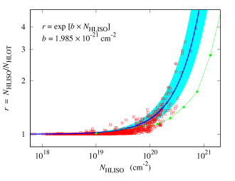
Figure 2: The ratio of “true” to apparent $N_{\rm HI}$ as a function of the true $N_{\rm HI}$. As $N_{\rm HI,ISO}$ is an unbiased estimate, we use that as a proxy for the true $N_{\rm HI}$. The observed data from individual velocity channels are shown as open squares. The thick line and the shaded region are the best fit exponential function with a factor of two uncertainty in the exponent. The filled squares joined by thin line is taken from simulations by Chengalur et al. (2013).

Based on this ${\it T}_{\rm B}-\tau$ correlation, we can define an estimator of $N_{\rm HI}$ using only ${\it T}_{\rm B,tot}$ for a velocity channel as

$$N_{\rm HI,E}=(1.823\times 10^{18}\>{\rm cm}^{-2})\>r({\it T}_{\rm B,tot})\>{\it T}_{\rm B,tot}dV\>,$$ (11)

where $dV$ is in ${\rm km~{}s}^{-1}$ and $r$ is a function of ${\it T}_{\rm B,tot}$ or $\tau_{\rm tot}$

$$r=N_{\rm HI,ISO}/N_{\rm HI,OT}=\frac{\tau_{\rm tot}}{\left[1-\exp(-\tau_{\rm tot})\right]}\>.$$ (12)

Figure 2 shows the observed ratio $r$ as a function of $N_{\rm HI,ISO}$ per $\sim 1\>{\rm km\>s^{-1}}$ velocity channel. We have used a fiducial functional form

$$r=r(N_{\rm HI,ISO})=1.00\>\exp(b\>N_{\rm HI,ISO})\>.$$ (13)

The best fit function and its variation for a factor of two change in the exponent $b$ are also shown in Figure 2. This functional form can now be used to iteratively solve equations (11) and (12) to get $N_{\rm HI,E}$ for the unit width velocity channel. To get the total $N_{\rm HI}$, $N_{\rm HI,E}$ should be summed over the full velocity range of the emission spectra. We have implemented this in a standard C code to estimate $N_{\rm HI}$ from emission line, and the results are shown in the next section.

4 Results and applications

This formalism to estimate $N_{\rm HI}$ from the $21$ cm emission spectra is applied to archival data from the LAB survey. In Figure 3, an example spectrum is shown to demonstrate the change in the estimated column density $N_{\rm HI,E}$ from the optically thin column density $N_{\rm HI,OT}$. The observed ${\it T}_{\rm B}=N_{\rm HI,OT}/1.823\times 10^{18}\>{\rm cm}^{-2}$ per $1\>{\rm km\>s^{-1}}$ velocity channel is shown as filled points joined by a line. The corrected estimate of $N_{\rm HI,E}$ per $1\>{\rm km\>s^{-1}}$ channel is shown as a thick line, and a pair of thin lines denote a factor of two uncertainty of the exponent $b$ in equation (13). For the example sightline ($l=20^{\circ}$, $b=6^{\circ}$), the $N_{\rm HI,OT}$ value is $2.87\times 10^{21}\>{\rm cm}^{-2}$, whereas the corrected $N_{\rm HI}$ value is $N_{\rm HI,E}=3.40\times 10^{21}\>{\rm cm}^{-2}$. The error in $N_{\rm HI}$ due to uncertainty in ${\it T}_{\rm B}$ is very small ($\sim 0.07\>{\rm K}=1.3\times 10^{17}\>{\rm cm}^{-2}$ per unit velocity interval). For an uncertainty in $b$ as large as a factor of two, the estimated $N_{\rm HI,E}$ changes by $\lesssim 20\%$ only.

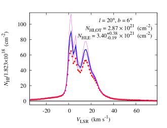
Figure 3: Example H i $21$ cm emission spectra from the LAB survey showing $N_{\rm HI}$ per $1$ km s^-1channel. The filled circles joined by line (the thick line) are $N_{\rm HI}$ before (after) correction for absorption (i.e. $N_{\rm HI,OT}$ and $N_{\rm HI,E}$ respectively). The uncertainty in $N_{\rm HI,E}$ (shown by the pair of thin lines) are for changing the exponent $b$ in equation (13) by a factor of two.

Next, we use the sample of Roy et al. (2013) to compare $N_{\rm HI,E}$ and $N_{\rm HI,ISO}$, and to check if $N_{\rm HI,E}$ is indeed an unbiased estimator as well. Please note that the ${\it T}_{\rm B}-\tau$ correlation used for this formalism is also from the same sample. However, $\tau$ varies for the sample by more than three orders of magnitude, and the observed correlation is between the averaged quantities. So, there is no a priori reason to expect the two column densities to match closely for the individual lines of sight. Figure 4 shows the fractional deviation of $N_{\rm HI,E}$ from $N_{\rm HI,ISO}$, $(N_{\rm HI,E}-N_{\rm HI,ISO})/N_{\rm HI,ISO}$, for this sample (filled circles with error bars). A similar fractional deviation between $N_{\rm HI,OT}$ and $N_{\rm HI,ISO}$ is also shown (open circles with error bars) for comparison. At lower $N_{\rm HI}$, all the estimates agree with each other. However, at higher $N_{\rm HI}$, $N_{\rm HI,E}$ matches better with $N_{\rm HI,ISO}$. This ascertains that $N_{\rm HI,E}$ is an useful and unbiased estimator of $N_{\rm HI}$ even when no absorption measurement is available.

We further extend this analysis to a larger sample for which both emission and absorption measurements are reported in the literature. However, in many cases, the velocity resolution of the data is coarse, and thus $N_{\rm HI,ISO}$ can not be computed reliably. One can, however, still estimate $N_{\rm HI,E}$, and combine it with the integrated optical depth from the literature to get the average ${\it T}_{\rm s}$ for the sightline. This is effectively the column density weighted harmonic mean of ${\it T}_{\rm s}$ ($\langle{\it T}_{\rm s}\rangle$) of different components along the sightline (Kulkarni & Heiles, 1988). The estimator is then applied to a sample of 318 sightlines, compiled from various H i absorption surveys after excluding non-detections and common sources: Dickey et al. (1983, 87 sources, spectral resolution $\Delta V=1.55$ km s^-1), Heiles & Troland (2003, 78 sources, $\Delta V=0.16$ km s^-1), Mohan et al. (2004, 102 sources, $\Delta V=3.3$ km s^-1), Liszt et al. (2010, 104 sources, $\Delta V=0.1$ km s^-1), and Roy et al. (2013, see above for details). These sightlines have the observed and interpolated $N_{\rm HI}$ in the range $\sim 8\times 10^{19}$ ${\rm cm}^{-2}$ to $2\times 10^{22}$ ${\rm cm}^{-2}$.

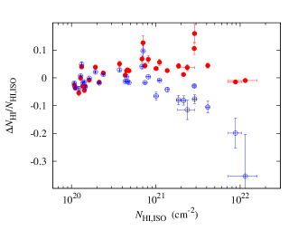
Figure 4: A comparison of different $N_{\rm HI}$ for Roy et al. (2013) sample. The filled circles show the fractional difference between $N_{\rm HI,E}$ and $N_{\rm HI,ISO}$, and the open circles show the fractional difference between $N_{\rm HI,E}$ and $N_{\rm HI,OT}$. The error bars include an assumed $20\%$ uncertainty in $N_{\rm HI,E}$.

As shown in the left panel of Figure 5, the estimated $N_{\rm HI}$ is $\sim 50\%$ higher than $N_{\rm HI,OT}$ when $N_{\rm HI,E}\gtrsim 10^{22}\>{\rm cm}^{-2}$. Comparing $N_{\rm HI,E}$ with $\int\tau\>dV$, the average ${\it T}_{\rm s}$ for most of these sightlines is between $100$ K and $1000$ K, with a trend of a lower ${\it T}_{\rm s}$ for higher $N_{\rm HI}$, as expected. This is shown in the right panel of Figure 5. We also see an indication of very low integrated optical depth at low $N_{\rm HI}$ (i.e. very high ${\it T}_{\rm s}$ and negligible cold gas fraction), suggesting a threshold column density of a few times $10^{20}\>{\rm cm}^{-2}$ for cold gas formation. Note that these trends are similar to what have been reported earlier by Kanekar et al. (2011) for a smaller sample.

Finally, the corrected column density $N_{\rm HI,E}$ can be well represented by a functional form

$$N_{\rm HI,E}=-A\ln\left(1-\frac{N_{\rm HI,OT}}{A}\right)\>\>,$$ (14)

suggested by Strasser & Taylor (2004). The best fit value of $A=(2.64\pm 0.06)\times 10^{22}$ cm^-2 for our sample is marginally different from the value $2.1\times 10^{22}$ cm^-2 reported for the Galactic plane by Strasser & Taylor (2004). We leave a more detailed analysis of a larger sample to model the observations in terms of the temperature of halo and disk gas of the Milky Way for future work.

5 Discussions and Conclusions

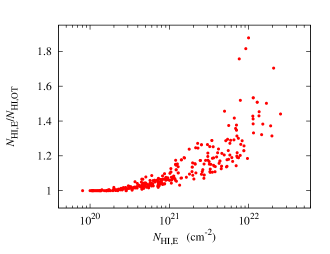
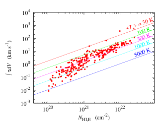
Figure 5: Left: A comparison of $N_{\rm HI,E}$ and $N_{\rm HI,OT}$ for a sample of Galactic sightlines. The difference is about $50\%$ for $N_{\rm HI,E}\gtrsim 10^{22}\>\>\>{\rm cm}^{-2}$. Right: The integrated optical depth as a function of $N_{\rm HI,E}$ for the same sample. Note that the average ${\it T}_{\rm s}$ is higher for low $N_{\rm HI}$ sightlines.

In this work, we have revisited the issue of estimating $N_{\rm HI}$ from H i $21$ cm absorption and emission spectra. Reliable estimation of $N_{\rm HI}$ from the emission spectra is challenging as the sightlines often pass through mix of gases at different temperature. Our knowledge of the relative position of these gas clouds is also limited. The issue is even more prominent at higher $\tau$; the derived $N_{\rm HI}$ is significantly biased because the optically thin limit underestimates the true $N_{\rm HI}$. Moreover, suitable continuum background source may not be present along the same or nearby sightlines for absorption studies.

We have developed a formalism to get an unbiased estimate of $N_{\rm HI}$ from only the emission spectrum, based on an observed correlation between ${\it T}_{\rm B}$ and $\tau$. The equivalent ${\it T}_{\rm s}-\tau$ correlation (${\it T}_{\rm s}\propto\tau^{-0.43}$) from the Roy et al. (2013) sample turns out to be in close agreement with that of previous studies (Lazareff, 1975; Heiles & Troland, 2003). However, to get the ${\it T}_{\rm s}-\tau$ correlation, these studies obtain the peak optical depth $\tau_{0}$ and the brightness temperature ${T_{{\rm B,peak}}}$ by modeling the spectrum with multiple Gaussians, and the parameters are thus model-dependent. Also, the low spectral resolution may lead to ambiguity in determining ${T_{{\rm B,peak}}}$ for Lazareff (1975). In contrast, our analysis and derived correlation is based on directly measured ${\it T}_{\rm B}(V)$ and $\tau(V)$ from all velocity channels. It should be noted that the observed ${\it T}_{\rm B}-\tau$ correlation only constrain a combination of $n$ and $\alpha$, namely $\alpha/(n-\alpha)$. In general, if $n\neq 1$, i.e. the assumption of thermal pressure equilibrium is not valid (Kulkarni & Heiles, 1988), the value of $\alpha$ will depend on $n$. This will, however, not affect any of the conclusions as we do not use $\alpha$ or $n$ separately in our analysis.

One caveat of the current study is that the ${\it T}_{\rm B}-\tau$ correlation is derived using measurements with very different spatial resolution. A good agreement of the observed ${\it T}_{\rm B}-\tau$ distribution with numerical simulations (Kim et al., 2014) indicates the broad consistency of our analysis. However, one would ideally like the resolution to be the same (which is practically hard to achieve), or systematically study the effect of a larger beam size for the emission spectra compared to the absorption spectra. For the complete sample of the absorption survey data, we plan to address this in the near future by deriving the ${\it T}_{\rm B}-\tau$ correlation, at least for a sub-sample, using emission spectra at different resolution (e.g. LAB survey, Effelsberg and Arecibo telescope data), and check how it affects the column density estimation.

The phase fraction distribution also affects the $N_{\rm HI}$ estimate obtained from the emission spectrum. Chengalur et al. (2013) carried out simulations with many different column density and gas temperature distributions to show that $N_{\rm HI,OT}$ is biased and underestimates $N_{\rm HI}$, while $N_{\rm HI,ISO}$ is an unbiased estimator. Even though their conclusion is qualitatively true, irrespective of what $N_{\rm HI}$ distribution is chosen, the ratio $r=N_{\rm HI,ISO}/N_{\rm HI,OT}$ quantitatively depends on the phase fraction and column density distributions. Hence, their simulation result on the variation of $r$ as a function of $N_{\rm HI,ISO}$ does not agree very well with our best fit function from observations, $r={\rm exp}[1.985\times 10^{-21}\ {\rm cm^{-2}}N_{\rm HI,ISO}]$, particularly for large $N_{\rm HI,ISO}$ values (see Figure 2). This is most likely due to the assumption that the sightlines pass through a random distribution of gas phases for their fiducial case. In reality, the actual phase fraction distribution may be very different from a random distribution, and can in principle be derived from the observed ${\it T}_{\rm B}-\tau$ correlation. Finally, once the effect of resolution is well-understood, this formalism may be extended for 21 cm observation of other galaxies to obtain an unbiased estimate of $N_{\rm HI}$, as well as to study $N_{\rm HI}$ distribution, power spectra etc. by using only the emission spectrum.

References

- Chengalur et al. (2013) Chengalur J. N., Kanekar N., Roy N., 2013, MNRAS, 432, 3074
- Clark et al. (1962) Clark B. G., Radhakrishnan V., Wilson R. W., 1962, ApJ, 135, 151
- Crovisier & Dickey (1983) Crovisier J. & Dickey J. M., 1983, A&A, 122, 282
- Dickey & Benson (1982) Dickey J. M. & Benson J. M., 1982, AJ, 87, 278
- Dickey et al. (1983) Dickey J. M., Kulkarni S. R., van Gorkom J. H., Heiles C. E., 1983, ApJS, 53, 591
- Dickey & Lockman (1990) Dickey J. M. & Lockman F. J., 1990, ARA&A, 28, 215
- Field (1965) Field G. B., 1965, ApJ, 142, 531
- Field et al. (1969) Field G. B., Goldsmith D. W., Habing H. J., 1969, ApJ, 155, L149
- Heiles & Troland (2003) Heiles C. & Troland T. H., 2003, ApJ, 586, 1067
- Kalberla et al. (2005) Kalberla P. M. W., Burton W. B., Hartmann D., Arnal E. M., Bajaja E., Morras R., Pöppel W. G. L., 2005, A&A, 440, 775
- Kanekar et al. (2011) Kanekar N., Braun R., Roy N., 2011, ApJ, 737, L33
- Kim et al. (2014) Kim C.-G., Ostriker E. C., Kim W.-T., 2014, ApJ, 786, 64
- Kulkarni & Heiles (1988) Kulkarni S. R., Heiles C., 1988, in Verschuur G. L., Kellermann K. I., eds, Galactic and Extra-Galactic Radio Astronomy Springer-Verlag New York, p. 95
- Lazareff (1975) Lazareff B., 1975, A&A, 42, 25
- Liszt (2001) Liszt H. S., 2001, A&A, 371, 698
- Liszt et al. (2010) Liszt H. S., Pety J., Lucas R., 2010, A&A, 518, A45
- Mohan et al. (2004) Mohan R., Dwarakanath K. S., Srinivasan G., 2004, JApA, 25, 143
- Roy et al. (2013) Roy N., Kanekar N., Braun R., Chengalur J. N., 2013, MNRAS, 436, 2352
- Strasser & Taylor (2004) Strasser S. & Taylor A. R., 2004, ApJ, 603, 560
- Walter et al. (2008) Walter F., Brinks E., de Blok W. J. G., Bigiel F., Kennicutt Jr. R. C., Thornley M. D., Leroy A., 2008, AJ, 136, 2563