The Sudakov radiator for jet observables and the soft physical coupling

Abstract

We present a procedure to calculate the Sudakov radiator for a generic recursive infrared and collinear (rIRC) safe observable in two-scale problems. We give closed formulae for the radiator at next-to-next-to-leading-logarithmic (NNLL) accuracy, which completes the general NNLL resummation for this class of observables in the ARES method for processes with two emitters at the Born level. As a byproduct, we define a physical coupling in the soft limit, and we provide an explicit expression for its relation to the $\overline{\rm MS}$ coupling up to ${\cal O}(\alpha_{s}^{3})$. This physical coupling constitutes one of the ingredients for a NNLL accurate parton shower algorithm. As an application we obtain analytic NNLL results, of which several are new, for all angularities $\tau_{x}$ defined with respect to both the thrust axis and the winner-take-all axis, and for the moments of energy-energy correlation $FC_{x}$ in $e^{+}e^{-}$ annihilation. For the latter observables we find that, for some values of $x$, an accurate prediction of the peak of the differential distribution requires a simultaneous resummation of the logarithmic terms originating from the two-jet limit and at the Sudakov shoulder.

1 Introduction

Distributions in event shapes and jet resolution parameters, collectively jet observables, are among the most studied QCD observables. Since they are continuous measures of the hadronic energy-momentum flow in jet events at colliders, they constitute a powerful probe of the dynamics of strong interactions, from high scales where fixed-order perturbative calculations can be applied, down to low scales where the yet unexplained phenomenon of hadronisation plays a decisive role.

Jet observables play a major role in measurements of the QCD coupling $\alpha_{s}$, and in testing non-perturbative hadronisation models (see e.g. Ref. Patrignani:2016xqp and references therein). The study of jet observables also led to important advances in the understanding of all-order properties of QCD radiation, which lead to the discovery of the so-called non-global logarithms NG1 ; NG2 ; Banfi:2002hw . Distributions in jet observables can be computed at fixed order in QCD perturbation theory. Such calculations have reached next-to-next-leading order (NNLO) accuracy for a number of relevant QCD processes. In particular, for $e^{+}e^{-}$ annihilation, NNLO corrections to three-jet production have been computed in refs. GehrmannDeRidder:2007hr ; GehrmannDeRidder:2008ug ; Weinzierl:2008iv ; Weinzierl:2009ms ; DelDuca:2016ily .

While fixed-order calculations provide a reliable tool to describe jet observables in the region where their values are large, the bulk of data lies in a region where multiple soft-collinear emissions give rise to large logarithms of the jet observable at all orders in perturbation theory. To be precise, given a generic jet observable, let us consider its cumulative distribution $\Sigma(v)$, the fraction of events such that the observable’s value is less than $v$. This quantity exhibits logarithmic terms as large as $\alpha_{s}^{n}L^{2n}$, where $L=-\ln v$ and $n$ is the order in QCD perturbation theory. Resumming those large logarithms means reorganising $\ln\Sigma$ in such a way that it can be written as $\alpha_{s}g_{1}(\alpha_{s}L)+g_{2}(\alpha_{s}L)+\alpha_{s}g_{3}(\alpha_{s}L)+\dots$, where $g_{1}(\alpha_{s}L)$ resums the so-called leading logarithmic (LL) contributions, $\alpha_{s}^{n}L^{n+1}$, $g_{2}(\alpha_{s}L)$ the NLL ones, $\alpha_{s}^{n}L^{n}$, $g_{3}(\alpha_{s}L)$ the NNLL ones, $\alpha_{s}^{n}L^{n-1}$, and so on.

Next-to-leading logarithmic (NLL) resummations, that include all terms ${\cal O}(\alpha_{s}^{n}L^{n})$ in the logarithm of cumulative distributions, have been available for many years for specific observables CSS ; CTTW ; Bonciani:2003nt ; thr_res ; mh_ee ; cpar_res ; DLMSBroadPT . Nowadays, NLL resummation for jet observables that have the properties of recursive infrared and collinear (rIRC) safety and continuous globalness Banfi:2004yd ; Banfi:2003je is a solved problem. The general solution is based on a semi-numerical approach developed for $e^{+}e^{-}$ event-shapes and jet rates in Ref. Banfi:2001bz , and later extended to any suitable jet observable in any QCD hard process Banfi:2004yd ; Banfi:2003je . The method is implemented in the computer program CAESAR Banfi:2004yd , that also verifies whether a given observable is rIRC safe and continuously global. This led to a first systematic study of event shapes in hadronic dijet production at NLL accuracy matched to next-to-leading order (NLO) results at hadron colliders Banfi:2004nk ; Banfi:2010xy .

NLL predictions have a sizeable theoretical uncertainty. Given the precision of current experiments, theoretical accuracy for resummations should aim at NNLL, and in some cases beyond. Most NNLL resummations are observable specific, and rely on the properties of the observable to achieve resummation through factorisation theorems that separate different kinematical configurations (e.g. hard, soft, collinear), and appropriate renormalisation group equations based on the fact that physical distributions do not depend on the unphysical scales that need to be introduced to achieve such separation. Such approaches made it possible to obtain full next-to-next-to-leading logarithmic (NNLL) predictions for a number of global $e^{+}e^{-}$ event shapes such as thrust $1-T$ Becher:2008cf ; Abbate:2010xh ; Monni:2011gb , heavy jet mass $\rho_{H}$ Chien:2010kc , jet broadenings $B_{T}$, $B_{W}$ Becher:2012qc , $C$-parameter Hoang:2014wka , energy-energy correlation (EEC) deFlorian:2004mp ; Tulipant:2017ybb ; Moult:2018jzp , heavy hemisphere groomed mass Frye:2016okc , and angularities Procura:2018zpn . Among the above examples, for $1-T$, $\rho_{H}$, $C$-parameter, and EEC, all N³LL corrections are also known, except for the four-loop cusp anomalous dimension, that has been computed numerically more recently Moch:2018wjh . Jet observables have been resummed at NNLL accuracy also in deep inelastic scattering Kang:2013nha ; Kang:2013wca ; Kang:2013lga . For hadronic collisions, full NNLL resummations are available for processes where a colour singlet is produced at Born level, specifically for a boson’s transverse momentum Bozzi:2005wk ; Becher:2010tm and $\phi^{*}$ Banfi:2011dx , the beam thrust Stewart:2010pd ; Berger:2010xi , transverse thrust Becher:2015lmy , and the leading jet’s transverse momentum Becher:2012qa ; Becher:2013xia ; Banfi:2012jm ; Stewart:2013faa , and for heavy quark pair’s transverse momentum Zhu:2012ts ; Catani:2014qha . For an arbitrary number of legs, a NNLL accurate resummation is available for the $N$-jettiness variable Jouttenus:2011wh . Very recently, resummations for the boson’s transverse momenta and $\phi^{*}$ have been pushed to N³LL accuracy Bizon:2017rah ; Bizon:2018foh ; Chen:2018pzu .

Despite these remarkable results, most jet observables are beyond the scope of factorisation theorems. This is especially true for those observables which cannot be expressed in terms of simple analytic functions of momenta, e.g. event shapes like the thrust major, or the two-jet rate in the Durham algorithm. For rIRC safe observables, it is possible to achieve NNLL accuracy by means of the semi-numerical method ARES (Automated Resummer for Event Shapes), developed for $e^{+}e^{-}$ event shapes in Ref. Banfi:2014sua , and later extended to jet rates Banfi:2016zlc . These publications focused on NNLL corrections induced by resolved real radiation. There, the cancellation of infrared singularities between unresolved real and virtual corrections to the Born process was parametrised in an observable dependent Sudakov form factor called “radiator”, that was extracted from existing calculations. This made it possible to study only observables that scale like powers of the transverse momentum or the invariant mass of the jet, which constitute a vast set of the phenomenologically relevant observables. This led to the first resummations for complicated observables such as the thrust major and the two-jet rate with various jet algorithms in $e^{+}e^{-}$ Banfi:2014sua ; Banfi:2016zlc .

In this paper we complete the last analytic ingredient necessary to have a fully general formula for the resummation of rIRC safe jet observables at NNLL in processes with two hard legs at the Born level. This makes it possible to handle all known observables of this type in a single framework, and hence paves the way to systematic phenomenological applications. We formulate the Sudakov radiator at all orders for a generic rIRC jet observable in QCD, and we explicitly compute it at NNLL accuracy. Our calculation of the Sudakov radiator must be then supplemented with the finite contributions coming from real radiation that are computed as in refs. Banfi:2014sua ; Banfi:2016zlc .

The paper is organised as follows. In section 2 we give the formulation of a general procedure for the resummation of jet observables with the ARES formalism. There we define the main object of our paper, the Sudakov radiator, which we compute at NNLL accuracy in section 3. The computation of the radiator leads to a definition of the physical coupling for soft radiation at higher orders. This generalises the scheme of Ref. Catani:1990rr , and constitutes an ingredient for future NNLL accurate parton shower algorithms. In that same section, we present a new formulation of the NNLL correction $\delta\mathcal{F}_{\rm correl}$ introduced in Ref. Banfi:2014sua , that we redefined in order to make sure that the Sudakov radiator can be computed analytically for an arbitrary rIRC safe jet observable. In section 4, we apply our method to angularities and moments of energy-energy correlation in $e^{+}e^{-}$ annihilation, and outline briefly the main features of their phenomenology at present and future colliders. Section 5 contains our conclusions.

2 Resummation in the ARES formalism

In this section we summarise the structure of the NNLL resummed cross section for a generic rIRC observable in $e^{+}e^{-}$ annihilation. We first set up the relevant notation and kinematics, and then we move on to derive the resummed cross section up to NNLL accuracy.

2.1 Kinematics and notation

Let $V(\{\tilde{p}\},k_{1},\dots,k_{n})$ be a generic continuously global, rIRC safe final-state observable, a function of all final-state momenta. Here $\{\tilde{p}\}$ denotes $\{\tilde{p}_{1},\tilde{p}_{2}\}$, which are the quark-antiquark pair initiating the process after all radiation has been emitted, and $k_{1},\dots,k_{n}$ are the momenta of the additional radiation. At Born level $V(\{\tilde{p}\})=0$. In order to parametrise the radiation momenta $k_{i}$, we introduce the following Sudakov decomposition

$$k_{i}^{\mu}=z_{i}^{(1)}p^{\mu}_{1}+z_{i}^{(2)}p^{\mu}_{2}+\kappa_{i}^{\mu},$$ (1)

where $p^{\mu}_{1},p^{\mu}_{2}$ are two light-like reference vectors, and $\kappa_{i}^{\mu}$ is a space-like four-vector and its magnitude is denoted by $k_{ti}\equiv\sqrt{-\kappa_{i}^{2}}$. The on-shell condition $k_{i}^{2}=0$ implies that $z_{i}^{(1)}z_{i}^{(2)}2(p_{1}p_{2})=k_{ti}^{2}$. The choice of the reference momenta $p_{1}$ and $p_{2}$ is arbitrary, and determines the mapping between the Sudakov variables $\{z_{i}^{(1)},z_{i}^{(2)},\kappa_{i}\}$ and the actual final-state momenta $\{\tilde{p}_{1},\tilde{p}_{2},k_{1},\dots,k_{n}\}$. A particular choice is therefore motivated by computational convenience. In our case, we observe that the product of the squared amplitude and phase space for an emission $k$ collinear to either $\tilde{p}_{1}$ or $\tilde{p}_{2}$ is proportional to

$$[dk]M^{2}(k)\propto\frac{d\tilde{k}_{t}^{2}}{\tilde{k}_{t}^{2}},\qquad{\rm where}\qquad{\tilde{k}}_{t}^{2}=\frac{2(\tilde{p}_{1}k)2(\tilde{p}_{2}k)}{2(\tilde{p}_{1}\tilde{p}_{2})}.$$ (2)

We choose the reference vectors $p_{1}$ and $p_{2}$ such that

$$\frac{dk_{t}^{2}}{k_{t}^{2}}=\frac{d\tilde{k}_{t}^{2}}{\tilde{k}_{t}^{2}}$$ (3)

up to corrections that vanish as a power of $k_{t}$ in the limit $k_{t}\to 0$. One possible solution, adopted in Ref. Banfi:2004yd , is to choose the two reference vectors $p_{1}$ and $p_{2}$ in Eq. (1) to be the momenta of the emitter of parton $k_{i}$ and the corresponding spectator. The precise definition of emitter and spectator requires specifying an ordering of insertion of the emissions in the event. A natural way of reconstructing the kinematics is to insert the emissions as follows:

• Start with the two-parton event consisting of the initial $q\bar{q}$ pair, without any additional emissions. These momenta define the initial $p_{1}$ and $p_{2}$ vectors.

• Consider a set of emissions parametrised by the triplet $\{z_{i}^{(1)},z_{i}^{(2)},\kappa_{i}\}$. At this stage the kinematics is not uniquely determined, as we did not specify the reference vectors of Eq. (1).

• Associate emissions for which $z_{i}^{(1)}>z_{i}^{(2)}$ to leg $\tilde{p}_{1}$, and emissions for which $z_{i}^{(2)}>z_{i}^{(1)}$ to leg $\tilde{p}_{2}$. For each emission $k_{i}$, define its rapidity $\eta_{i}$ with respect to the emitting leg as

  $$\eta_{i}^{(1)} =\frac{1}{2}\ln\frac{z_{i}^{(1)}}{z_{i}^{(2)}}\,,\quad{\rm if}\quad z_{i}^{(1)}>z_{i}^{(2)}\,,$$ (4)

  $$\eta_{i}^{(2)} =\frac{1}{2}\ln\frac{z_{i}^{(2)}}{z_{i}^{(1)}}\,,\quad{\rm if}\quad z_{i}^{(1)}<z_{i}^{(2)}\,.$$ (5)

• For each leg $\ell$, insert the emissions into the initial event starting from the one at smaller $\eta^{(\ell)}$. The reference momentum $p_{\ell}$ in Eq. (1) represents the emitter and takes the transverse recoil. The longitudinal recoil is shared between the emitter and a spectator momentum (i.e. the remaining reference vector in Eq. (1)). However, for the purpose of the analytical method presented in this paper, one can safely neglect the longitudinal recoil of the spectator (which is proportional to $k_{ti}^{2}$) that would otherwise give rise to regular terms in the cross section. For instance, for an emission $k$ emitted off leg $1$, and parametrised by Eq. (1), we have

  $$p_{1}^{\mu}\to(1-z^{(1)})p_{1}^{\mu}-\kappa^{\mu}\,,\qquad p_{2}^{\mu}\to p_{2}^{\mu}.$$ (6)

  The resulting momenta $p_{1}$ and $p_{2}$, after the emission, will be massless up to ${\cal O}(k_{ti}^{2})$ corrections.

• Update the reference momenta, and proceed with the insertion of emissions at progressively larger $\eta_{i}^{(\ell)}$.

This procedure guarantees the validity of Eq. (3), and implies that the reference vectors $p_{1}$ and $p_{2}$ are different for each emission Banfi:2014sua .

Before proceeding, we stress that the ordering chosen for the insertion of the emissions in the event has nothing to with the way the triplets $\{z_{i}^{(1)},z_{i}^{(2)},\kappa_{i}\}$ are produced. For instance, when computing the resummation via a Monte Carlo algorithm, it is convenient to generate this triplet according to an ordering in the observable’s value (see, e.g. Banfi:2004yd ; Banfi:2014sua ). This ordering is however unrelated to the ordering with which the emissions are inserted, which follows the angular ordering arguments outlined above. This is essential to specify a correct recoil scheme that preserves the simple factorised form of QCD matrix elements.

2.2 General structure of NNLL resummation

Any rIRC safe observable $V(\{\tilde{p}\},k_{1},\dots,k_{n})$, can be parametrised in the following way for a single soft and collinear emission $k$ collinear to each leg $\ell$

$$V(\{\tilde{p}\},k)\simeq V_{\text{sc}}(k)\equiv\sum_{\ell=1}^{2}d_{\ell}\left(\frac{k_{t}^{(\ell)}}{Q}\right)^{a}e^{-b_{\ell}\eta^{(\ell)}}g_{\ell}(\phi^{(\ell)})\Theta(\eta^{(\ell)})\,.$$ (7)

Here $k_{t}^{(\ell)},\eta^{(\ell)},\phi^{(\ell)}$ are the transverse momentum, rapidity and azimuth of $k$ with respect to the emitter $p_{\ell}$ as defined in the previous section, whereas $a,b_{\ell},d_{\ell}$ are constants. The scale $Q$ represents a typical hard scale of the process, in our case the centre-of-mass energy of the $e^{+}e^{-}$ collision.

Our aim is to resum large logarithms in the cumulative distribution $\Sigma(v)$, the fraction of events for which $V(\{\tilde{p}\},k_{1},\dots,k_{n})<v$, in the region $v\ll 1$. This is given by

$$\Sigma(v)\equiv\frac{1}{\sigma}\int_{0}^{v}dv^{\prime}\frac{d\sigma(v^{\prime})}{dv^{\prime}}=\mathcal{H}(Q)\sum_{n=0}^{\infty}\frac{1}{n!}\int\prod_{i=1}^{n}[dk_{i}]\mathcal{M}^{2}(k_{1},...,k_{n})\Theta(v-V(\{\tilde{p}\},k_{1},\dots,k_{n}))\,,$$ (8)

where $\mathcal{H}(Q)$ includes all virtual corrections to the Born process (normalised to the total cross section $\sigma$) and $\mathcal{M}^{2}(k_{1},...,k_{n})$ is the amplitude squared for $n$ real emissions. The Lorentz-invariant phase-space in $d=4-2\epsilon$ dimensions is denoted by $[dk]$ and defined as

$$[dk]\equiv\frac{d^{d}k}{(2\pi)^{d-1}}\delta(k^{2})\Theta(k^{0}).$$ (9)

Given the Sudakov decomposition of any four-momentum $k$ of (squared) invariant mass $k^{2}=m^{2}$ as in Eq. (1), the measure $d^{d}k$ can be expressed as

$$d^{d}k=(p_{1}p_{2})dz^{(1)}dz^{(2)}d^{2-2\epsilon}k_{t}=\frac{dy}{2}dm^{2}d^{2-2\epsilon}k_{t},\qquad y\equiv\frac{1}{2}\ln\left(\frac{z^{(1)}}{z^{(2)}}\right)\,.$$ (10)

The variable $y$ is the rapidity of $k$ (with respect to some reference light-like directions $p_{1}$ and $p_{2}$), and for real emissions, i.e. $k^{2}=0$, it is bounded by

$$|y|<\ln\left(\frac{Q}{k_{t}}\right)\,.$$ (11)

It is immediate to link $y$ to the rapidity of a massless emission $k$ with respect to a given leg $\ell$. In fact, $\eta^{(1)}=y$ for $y>0$, and $\eta^{(2)}=-y$ for $y<0$. This implies that the phase space $[dk]$ in Eq. (9) can be written as follows

$$[dk]=\sum_{\ell=1}^{2}\frac{d\eta^{(\ell)}}{2}\Theta(\eta^{(\ell)})\frac{d^{2-2\epsilon}k_{t}}{(2\pi)^{3-2\epsilon}}\,.$$ (12)

So far, all momenta have to be considered in $d$-dimensions, because dimensional regularisation is needed to regulate the IRC divergences present both in $\mathcal{H}(Q)$ and in the real radiation.

The virtual corrections $\mathcal{H}(Q)$ can be expressed as Laenen:2000ij ; Dixon:2008gr

$$\mathcal{H}(Q)=C(\alpha_{s}(Q)) \exp\left\{-\int\frac{d^{d}k}{(2\pi)^{d}}\,w(m^{2},k_{t}^{2}+m^{2};\epsilon)\,\Theta\left(\frac{1}{2}\ln\left(\frac{Q^{2}}{k_{t}^{2}+m^{2}}\right)-|y|\right)\Theta(Q-k_{t})\right\}\times$$

$$\times\exp\left\{-\sum_{\ell=1}^{2}\int^{Q^{2}}\frac{dk^{2}}{k^{2}}\gamma_{\ell}(\alpha_{s}(k,\epsilon))\right\}\ \ .$$ (13)

The virtual corrections are parametrised in three objects. First, $w(m^{2},k_{t}^{2}+m^{2};\epsilon)$ denotes the soft web FT ; NAET of total momentum $k$ and squared invariant mass $m^{2}$, in $d=4-2\epsilon$ dimensions. The web is obtained by considering the Feynman graphs with two eikonal lines that cannot be further decomposed into subgraphs by cutting each eikonal line once. For example, at lowest order in perturbation theory we find

$$w^{(1)}(m^{2},m^{2}+k_{t}^{2};\epsilon)=(4\pi)^{2}\frac{2C_{\ell}}{k_{t}^{2}}\mu_{R}^{2\epsilon}\alpha_{s}(\mu_{R})\delta(m^{2})\,,$$ (14)

where $C_{\ell}=C_{F}$ in the case of quarks, and $C_{\ell}=C_{A}$ in the case of emitting gluons. Note that the web does not depend on the rapidity $y$, due to the properties of eikonal Feynman rules. Remarkably, at each order in perturbation theory, the web has a finite limit for $\epsilon\to 0$, which we will simply denote by $w(m^{2},m^{2}+k_{t}^{2})$. Second, the function $\gamma_{\ell}(\alpha_{s}(k,\epsilon))$ coincides, up to an overall sign change, with the coefficient of the $\delta(1-x)$ term of the regularised splitting functions $P_{qq}(x)$ and $P_{gg}(x)$, according to whether leg $\ell$ is a quark or a gluon, respectively. The strong coupling $\alpha_{s}(k,\epsilon)$ is defined as the solution of the $d$-dimensional renormalisation group equation:

$$\mu_{R}^{2}\frac{d\alpha_{s}}{d\mu_{R}^{2}}=-\epsilon\,\alpha_{s}+\beta^{\rm(d=4)}(\alpha_{s}),$$ (15)

where $\beta^{\rm(d=4)}$ is the beta function in four dimensions, given by the following expansion

$$\beta^{\rm(d=4)}(\alpha_{s})=-\alpha_{s}^{2}\sum_{n=0}^{\infty}\beta_{n}\alpha_{s}^{n}\,.$$ (16)

In our representation of $\mathcal{H}(Q)$, the upper integration bound for the $k_{t}$-integral of the web is set by the centre-of-mass energy $Q$, and the upper bound for the rapidity integral to $|y|<\ln(Q/\sqrt{k_{t}^{2}+m^{2}})$. Finally, the overall quantity $C(\alpha_{s}(Q))$ is a multiplicative constant that is obtained by matching Eq. (2.2) at each order in perturbation theory to the quark or gluon form factor computed in the $\overline{\rm MS}$ scheme.

In order to proceed, we need to define a procedure to cancel the IRC singularities in Eq. (2.2) against those in the real emissions. This can be done by introducing a resolution parameter that is engineered in such a way to divide the real radiation into a resolved set and an unresolved one. The idea behind this procedure is to handle the unresolved part of the radiation analytically, and hence cancel the divergences against the virtual corrections. The cancellation is performed in a manner that the resolved contributions could subsequently be computed numerically in $d=4$ dimensions. The resolution parameter is defined through its action on the soft and/or hard-collinear contributions to the squared amplitudes, as outlined below.

We start by considering soft radiation. The soft squared amplitudes for $n$ emissions, denoted hereafter as $M_{\rm s}^{2}(k_{1},\dots,k_{n})$, can be iteratively reorganised as follows

$$M_{\rm s}^{2}(k_{1}) \equiv\tilde{M}_{\rm s}^{2}(k_{1})$$

$$M_{\rm s}^{2}(k_{1},k_{2}) =\tilde{M}_{\rm s}^{2}(k_{1})\tilde{M}_{\rm s}^{2}(k_{2})+\tilde{M}_{\rm s}^{2}(k_{1},k_{2})$$

$$M_{\rm s}^{2}(k_{1},k_{2},k_{3}) =\tilde{M}_{\rm s}^{2}(k_{1})\tilde{M}_{\rm s}^{2}(k_{2})\tilde{M}_{\rm s}^{2}(k_{3})+\left(\tilde{M}_{\rm s}^{2}(k_{1})\tilde{M}_{\rm s}^{2}(k_{2},k_{3})+\text{perm.}\right)+\tilde{M}_{\rm s}^{2}(k_{1},k_{2},k_{3})\,$$

$$\vdots$$ (17)

The quantities $\tilde{M}_{\rm s}^{2}(k_{1},\dots,k_{n})$ represent the correlated portion of the $n$-emission soft amplitude squared, together with its virtual corrections. This is strongly suppressed unless all emissions $k_{1},\dots,k_{n}$ are close in angle. We refer to the latter as soft correlated blocks and they play a dominant role in constructing the webs, which are the building objects of the Sudakov radiator to be defined below. Each correlated block admits a perturbative expansion in $\alpha_{s}$ due to virtual corrections, hence

$$\tilde{M}_{\rm s}^{2}(k_{1},\dots,k_{n})=\tilde{M}_{\rm s,0}^{2}(k_{1},\dots,k_{n})+\frac{\alpha_{s}(\mu_{R})}{2\pi}\tilde{M}_{\rm s,1}^{2}(k_{1},\dots,k_{n})+\dots$$ (18)

For instance, at tree level, the squared matrix element for the emission of a single soft gluon is given by

$$\tilde{M}_{\rm s}^{2}(k)\simeq\tilde{M}_{\rm s,0}^{2}(k)=16\pi\,C_{\ell}\,\mu_{R}^{2\epsilon}\frac{\alpha_{s}(\mu_{R})}{k_{t}^{2}},$$ (19)

while at one-loop order one has Catani:2000pi

$$\tilde{M}_{\rm s,1}^{2}(k)=-\tilde{M}_{\rm s,0}^{2}(k)C_{A}\frac{1}{\epsilon^{2}}\frac{\Gamma^{4}(1-\epsilon)\Gamma^{3}(1+\epsilon)}{\Gamma^{2}(1-2\epsilon)\Gamma(1+2\epsilon)}\left(\frac{4\pi\mu_{R}^{2}}{k_{t}^{2}}\right)^{\epsilon}.$$ (20)

In the following the coupling will be always renormalised in the $\overline{\rm MS}$ scheme, i.e. we replace

$$\mu_{R}^{2\epsilon}\alpha_{s}(\mu_{R})\to\mu_{R}^{2\epsilon}\alpha_{s}(\mu_{R})\frac{e^{\epsilon\gamma_{E}}}{(4\pi)^{\epsilon}}\left(1-\frac{\beta_{0}}{\epsilon}\alpha_{s}(\mu_{R})+\dots\right)\,,$$ (21)

where $\beta_{0}$ is the first coefficient of the beta function in four dimensions of Eq. (16), given by

$$\beta_{0}=\frac{11C_{A}-2n_{f}}{12\pi}\,.$$ (22)

The tree-level correlated block with two emissions $\tilde{M}_{\rm s,0}^{2}(k_{1},k_{2})$ is reported in Appendix A, and will be useful later. This decomposition is particularly convenient to define a logarithmic counting. Each correlated block $\tilde{M}_{\rm s}^{2}(k_{1},\dots,k_{n})$ will contribute to $\ln\Sigma(v)$ at most with a factor $\alpha_{s}^{n}\ln^{n+1}(v)$, with $n$ powers of $\ln(v)$ coming from the soft singularities and an extra power from the only collinear singularity.

The definition of the resolution parameter proceeds as follows. First, we define a clustering algorithm that combines together the momenta of all particles emitted according to each correlated block $\tilde{M}_{\rm s}^{2}(k_{1},\dots,k_{n})$. For example consider the simple case of two emissions, the clustering is assigned as follows

$$M_{\rm s}^{2}(k_{1},k_{2})=\underbrace{\tilde{M}_{\rm s}^{2}(k_{1})\tilde{M}_{\rm s}^{2}(k_{2})}_{\text{ two clusters }(k_{1},k_{2})}\qquad+\underbrace{\tilde{M}_{\rm s}^{2}(k_{1},k_{2})}_{\text{a single cluster }k_{\text{clust.}}=k_{1}+k_{2}}\ \ .$$ (23)

The property of rIRC safety Banfi:2004yd implies that all particles in a cluster are both close in angle and have commensurate transverse momenta. This allows one to evaluate the QCD running couplings of each cluster at the transverse momenta of the corresponding emissions. This procedure allows us to absorb all logarithms of $\mu_{R}/k_{ti}$ into the running of the coupling. As a consequence of this procedure, for rIRC safe observables, using the decomposition (17), every correlated block $\tilde{M}_{\rm s}^{2}(k_{1},\dots,k_{n})$ (when combined with the corresponding virtual corrections) will contribute to $\ln\Sigma(v)$ with terms of order $\alpha_{s}^{m}\ln^{m+2-n}(v)$ for $m\geq n$. This allows us to build a logarithmic counting at the level of the squared amplitude, which defines which contributions must be considered at a given logarithmic order.

In order to proceed with the calculation of $\Sigma(v)$, we then choose a resolution parameter $\delta\ll 1$ such that all clusters of total momentum $k_{\text{clust.}}$ satisfying

$$V_{\text{sc}}(k_{\text{clust.}})<\delta v\,,\$$ (24)

are labelled as unresolved. This choice guarantees that one is able to compute analytically the contribution of unresolved emissions for an arbitrary rIRC safe observable. For this class of observables, the unresolved clusters can be neglected from the $\Theta$ function in Eq. (8) since they do not contribute to the observable $V$ up to corrections suppressed by powers of $\delta^{p}v$, with $p$ being a positive parameter.

The above definition of the resolution parameter allows us to exponentiate the contribution of unresolved soft blocks. From the decomposition of Eq. (17), it is straightforward to connect the correlated blocks $\tilde{M}_{\rm s}^{2}(k_{1},\dots,k_{n})$ to the webs introduced in Eq. (2.2). In fact

$$w(m^{2},k_{t}^{2}+m^{2};\epsilon)=\sum_{n=1}^{\infty}S(n)\int\left(\prod_{i=1}^{n}[dk_{i}]\right)\tilde{M}_{\rm s}^{2}(k_{1},...,k_{n})(2\pi)^{d}\delta^{(d)}(k-\sum_{i}k_{i})\,,$$ (25)

where the factor $S(n)$ represents the multiplicity coefficient for each soft final state (quarks or gluons). For instance, for $n$ identical gluons, $S(n)=1/n!$. Therefore, the contribution of an arbitrary number of soft clusters (and no hard-collinear clusters) gives rise to the following exponential factor

$$\exp\left\{\int^{Q}\frac{d^{d}k}{(2\pi)^{d}}w(m^{2},k_{t}^{2}+m^{2};\epsilon)\Theta(\delta v-V_{\rm sc}(k))\right\}\,.$$ (26)

Eq. (26) can be promptly combined with the virtual corrections in (2.2) to give

$$\mathcal{H}(Q)\exp\left\{\int^{Q}\frac{d^{d}k}{(2\pi)^{d}}w(m^{2},k_{t}^{2}+m^{2};\epsilon)\Theta(\delta v-V_{\rm sc}(k))\right\}$$

$$=C(\alpha_{s}(Q))e^{-R_{\rm s}(\delta v)}\exp\left\{-\sum_{\ell=1}^{2}\int^{Q^{2}}\frac{dk^{2}}{k^{2}}\gamma_{\ell}(\alpha_{s}(k,\epsilon))\right\}\,,$$ (27)

where we defined the soft radiator $R_{\rm s}$ as

$$R_{\rm s}(v)=\int^{Q}\frac{d^{4}k}{(2\pi)^{4}}w(m^{2},k_{t}^{2}+m^{2})\Theta(V_{\rm sc}(k)-v)\,,$$ (28)

and we took the four-dimensional limit of the web (and the relative integration measure) since the integral is now finite.

The next step is to handle the remaining hard-collinear divergences present in the integral over $\gamma$ in Eq. (27). Unlike the case of soft radiation, the exponentiation of the unresolved hard-collinear emissions is more delicate in that every hard-collinear emission could potentially change the colour charge felt by subsequent radiation. However, the treatment of hard-collinear radiation is much simplified by observing that, owing to rIRC safety, only a fixed number of hard-collinear emissions is to be considered at a given logarithmic order. Therefore, instead of proceeding as in the soft case, it is convenient to start from the integral over the anomalous dimension $\gamma$ in the virtual corrections (27) and split it into two pieces at the collinear scale of the resolution variable, that is found by setting the rapidity $\eta^{(\ell)}$ to its maximum (i.e. $\ln(Q/k_{t}))$ in Eq. (7), which yields $V_{\rm sc}(k)\sim k_{t}^{a+b_{\ell}}$. Inspired by this, the integral over $\gamma$ then can be split at $k=v^{1/(a+b_{\ell})}Q$ and becomes

$$\int^{Q^{2}}\frac{dk^{2}}{k^{2}}\gamma_{\ell}(\alpha_{s}(k,\epsilon))=\int^{Q^{2}}_{Q^{2}v^{\frac{2}{a+b_{\ell}}}}\frac{dk^{2}}{k^{2}}\gamma_{\ell}(\alpha_{s}(k))+\int^{Q^{2}v^{\frac{2}{a+b_{\ell}}}}_{0}\frac{dk^{2}}{k^{2}}\gamma_{\ell}(\alpha_{s}(k,\epsilon))\,.$$ (29)

Next, we expand the exponential of the second integral in the r.h.s. of the above equation considering only a fixed number of terms in its expansion as

$$\exp\left\{-\int^{Q^{2}v^{\frac{2}{a+b_{\ell}}}}_{0}\frac{dk^{2}}{k^{2}}\gamma_{\ell}(\alpha_{s}(k,\epsilon))\right\}=1-\int^{Q^{2}v^{\frac{2}{a+b_{\ell}}}}_{0}\frac{dk^{2}}{k^{2}}\frac{\alpha_{s}(k,\epsilon)}{2\pi}\gamma^{(0)}_{\ell}+{\cal O}(\alpha_{s}^{2}(Qv^{\frac{1}{a+b_{\ell}}})),$$ (30)

where, in our case of emitting quarks, the leading-order anomalous dimension is given by

$$\gamma^{(0)}_{\ell}=-\frac{3}{2}\,C_{F}.$$ (31)

The first non-trivial order in the expansion must be included at NNLL, the second at N³LL (together with the squared of the first), and so forth. The divergences of these terms will cancel order-by-order in perturbation theory against those of the hard-collinear emissions in the real radiation.

The last step to obtain a NNLL expression for $\Sigma(v)$ is to handle the squared matrix element for real emissions ${\cal M}^{2}$ in Eq. (8). At NLL accuracy, rIRC safety ensures that resolved radiation contains no hard-collinear emissions, and the real matrix element squared is approximated by its soft approximation $M_{\rm s}^{2}$. Moreover, the squared amplitude at this order reduces to the product of $n$ independent, soft-collinear emission probabilities. In fact, $[dk]M_{\rm s,0}^{2}(k)\simeq[dk]M^{2}_{\rm sc}(k)$, where Banfi:2014sua

$$[dk]M^{2}_{\rm sc}(k)\equiv\sum_{\ell=1,2}2C_{\ell}\frac{\alpha_{s}(k^{(\ell)}_{t})}{\pi}\frac{dk^{(\ell)}_{t}}{k^{(\ell)}_{t}}d\eta^{(\ell)}\,\Theta\left(\ln\left(\frac{Q}{k^{(\ell)}_{t}}\right)-\eta^{(\ell)}\right)\Theta(\eta^{(\ell)})\frac{d\phi^{(\ell)}}{2\pi}\,,$$ (32)

and $C_{\ell}$ the colour factor of leg $\ell$, $C_{F}$ for a quark and $C_{A}$ for a gluon. In order to achieve NNLL accuracy, it is sufficient to correct the products of independently emitted single-particle clusters with the insertion of a single tree-level correlated cluster of two soft and collinear emissions $\tilde{M}_{\rm s,0}^{2}(k_{a},k_{b})$, and of the one-loop correction to the single-emission cluster $\tilde{M}_{\rm s,1}^{2}(k)$.

Moreover, beyond NLL, a finite number of hard-collinear emissions must be considered. In particular, at NNLL, it is sufficient to allow one single emission to be hard and collinear. When combined with Eq. (30), this leads to a finite, logarithmically enhanced, left over, as it will be shown shortly. In such configurations, at NNLL, the remaining soft radiation consists of an arbitrary number of single-emission clusters.

With the above decomposition, the NNLL resummed cross section $\Sigma(v)$ of Eq. (8) takes the form

$$\Sigma_{\rm NNLL}(v)=C(\alpha_{s}(Q))e^{-R_{\rm s}(\delta v)}\exp\left\{-\sum_{\ell=1}^{2}\int^{Q^{2}}_{Q^{2}v^{\frac{2}{a+b_{\ell}}}}\frac{dk^{2}}{k^{2}}\gamma_{\ell}(\alpha_{s}(k))\right\}$$

$$\times\bigg{\{}\sum_{n=0}^{\infty}\frac{1}{n!}\int\prod_{i=1}^{n}[dk_{i}]M_{\rm s}^{2}(k_{1},...,k_{n})\Theta(v-V(\{\tilde{p}\},k_{1},\dots,k_{n}))\prod_{\rm clust.}\Theta\left(V_{\rm sc}(k_{\rm clust.})-\delta v\right)$$

$$+\sum_{n=0}^{\infty}\frac{1}{n!}\int\prod_{i=1}^{n}[dk_{i}]M_{\rm sc}^{2}(k_{i})\Theta\left(V_{\rm sc}(k_{i})-\delta v\right)\times\sum_{\ell=1}^{2}\bigg{[}\int[dk_{\rm hc}]M_{\rm hc,\ell}^{2}(k_{\rm hc})\Theta(v-V(\{\tilde{p}\},k_{1},\dots,k_{n},k_{\rm hc}))$$

$$-\int^{Q^{2}v^{\frac{2}{a+b_{\ell}}}}_{0}\frac{dk^{2}}{k^{2}}\frac{\alpha_{s}(k,\epsilon)}{2\pi}\gamma^{(0)}_{\ell}\Theta(v-V(\{\tilde{p}\},k_{1},\dots,k_{n}))\bigg{]}\bigg{\}},$$ (33)

where the squared amplitude $M_{\rm s}^{2}(k_{1},...,k_{n})$ is approximated by

$$\begin{split}M_{\rm s}^{2}(k_{1},...,k_{n})&\prod_{\rm clust.}\Theta\left(V_{\rm sc}(k_{\rm clust.})-\delta v\right)\simeq\prod_{i=1}^{n}M_{\rm sc}^{2}(k_{i})\Theta\left(V_{\rm sc}(k_{i})-\delta v\right)\\ &+\sum_{a>b}\prod_{\begin{subarray}{c}i=1\\ i\neq a,b\end{subarray}}^{n}M_{\rm sc}^{2}(k_{i})\Theta\left(V_{\rm sc}(k_{i})-\delta v\right)\tilde{M}_{\rm s,0}^{2}(k_{a},k_{b})\Theta\left(V_{\rm sc}(k_{a}+k_{b})-\delta v\right)\\ &+\frac{\alpha_{s}(\mu_{R})}{2\pi}\sum_{a}\prod_{\begin{subarray}{c}i=1\\ i\neq a\end{subarray}}^{n}M_{\rm sc}^{2}(k_{i})\Theta\left(V_{\rm sc}(k_{i})-\delta v\right)\tilde{M}_{\rm s,1}^{2}(k_{a})\Theta\left(V_{\rm sc}(k_{a})-\delta v\right)\,,\end{split}$$ (34)

where $V_{\rm sc}(k_{a}+k_{b})$ is defined as in Eq. (7), and $k_{t}^{(\ell)},\eta^{(\ell)},\phi^{(\ell)}$ are the transverse momentum, rapidity and azimuth of the four-vector $k_{a}+k_{b}$ with respect to leg $\ell$. The cancellation of infrared and collinear divergences in the first term of Eq. (2.2) can be easily handled with a simple subtraction scheme as outlined in Ref. Banfi:2014sua , which allows for a numerical evaluation in $d=4$ dimensions. The cancellation of collinear singularities in the second term still requires the use of dimensional regularisation. In order to make the second term suitable for a numerical evaluation, we add and subtract the following counter-term

$$C(\alpha_{s}(Q)) e^{-R_{\rm s}(\delta v)}\exp\left\{-\sum_{\ell=1}^{2}\int^{Q^{2}}_{Q^{2}v^{\frac{2}{a+b_{\ell}}}}\frac{dk^{2}}{k^{2}}\gamma_{\ell}(\alpha_{s}(k,\epsilon))\right\}$$

$$\times\sum_{n=0}^{\infty}\frac{1}{n!}\int\prod_{i=1}^{n}[dk_{i}]M_{\rm sc}^{2}(k_{i})\Theta\left(V_{\rm sc}(k_{i})-\delta v\right)$$

$$\times\sum_{\ell=1}^{2}\int[dk_{\rm hc}]M_{\rm hc,\ell}^{2}(k_{\rm hc})\Theta(v-V(\{\tilde{p}\},k_{1},\dots,k_{n}))\Theta(v-V_{\rm sc}(k_{\rm hc})),$$ (35)

and recast Eq. (2.2) as follows

$$\Sigma(v)=C(\alpha_{s}(Q))e^{-R_{\rm s}(\delta v)}\exp\left\{-\sum_{\ell=1}^{2}\int^{Q^{2}}_{Q^{2}v^{\frac{2}{a+b_{\ell}}}}\frac{dk^{2}}{k^{2}}\gamma_{\ell}(\alpha_{s}(k,\epsilon))\right\}$$

$$\times\bigg{\{}\sum_{n=0}^{\infty}\frac{1}{n!}\int\prod_{i=1}^{n}[dk_{i}]M_{\rm s}^{2}(k_{1},...,k_{n})\Theta(v-V(\{\tilde{p}\},k_{1},\dots,k_{n}))\prod_{\rm clust.}\Theta\left(V_{\rm sc}(k_{\rm clust.})-\delta v\right)$$

$$+\sum_{n=0}^{\infty}\frac{1}{n!}\int\prod_{i=1}^{n}[dk_{i}]M_{\rm sc}^{2}(k_{i})\Theta\left(V_{\rm sc}(k_{i})-\delta v\right)$$

$$\times\sum_{\ell=1}^{2}\bigg{[}\int[dk_{\rm hc}]M_{\rm hc,\ell}^{2}(k_{\rm hc})\bigg{(}\Theta(v-V(\{\tilde{p}\},k_{1},\dots,k_{n},k_{\rm hc}))-\Theta(v-V(\{\tilde{p}\},k_{1},\dots,k_{n}))\Theta(v-V_{\rm sc}(k_{\rm hc}))\bigg{)}$$

$$+\bigg{(}\int[dk_{\rm hc}]M_{\rm hc,\ell}^{2}(k_{\rm hc})\Theta(v-V_{\rm sc}(k_{\rm hc}))-\int^{Q^{2}v^{\frac{2}{a+b_{\ell}}}}_{0}\frac{dk^{2}}{k^{2}}\frac{\alpha_{s}(k,\epsilon)}{2\pi}\gamma^{(0)}_{\ell}\bigg{)}\Theta(v-V(\{\tilde{p}\},k_{1},\dots,k_{n}))\bigg{]}\bigg{\}}.$$ (36)

The integral in round brackets of the last line of the above equation can be evaluated analytically as follows. For each leg $\ell=1,2$, we expand the $\Theta(v-V_{\rm sc}(k_{\rm hc}))$ function in the last line of Eq. (2.2) as

$$\Theta(v-V_{\rm sc}(k_{\rm hc})) =\Theta\left(v-d_{\ell}\left(\frac{k_{t}^{(\ell)}}{Q}\right)^{a}e^{-b_{\ell}\eta^{(\ell)}}g_{\ell}(\phi^{(\ell)})\right)=\Theta\left(v-\left(\frac{k_{t}^{(\ell)}}{Q}\right)^{a+b_{\ell}}\frac{d_{\ell}g_{\ell}(\phi^{(\ell)})}{(z^{(\ell)})^{b_{\ell}}}\right)$$

$$=\Theta\left(v-\left(\frac{k_{t}^{(\ell)}}{Q}\right)^{a+b_{\ell}}\right)-v\,\delta\left(v-\left(\frac{k_{t}^{(\ell)}}{Q}\right)^{a+b_{\ell}}\right)\ln\frac{d_{\ell}g_{\ell}(\phi^{(\ell)})}{(z^{(\ell)})^{b_{\ell}}}+\dots$$ (37)

where we neglect N³LL corrections in the expansion.

With the above expansion it is sufficient to use the azimuthally averaged splitting function in $d=4-2\epsilon$ dimensions to construct the hard-collinear squared matrix element, since in Eq. (2.2) the only term that involves a non-trivial $\phi^{(\ell)}$ dependence is finite in $d=4$ dimensions. In this approximation, the hard-collinear emission probability relative to each leg $\ell$ is given by

$$[dk]M_{\rm hc,\ell}^{2}(k)=2\frac{e^{\gamma_{E}\epsilon}}{\Gamma(1-\epsilon)}\frac{dk_{t}^{(\ell)}}{k_{t}^{(\ell)}}\left(\frac{\mu_{R}}{k_{t}^{(\ell)}}\right)^{2\epsilon}dz^{(\ell)}\frac{d\phi^{(\ell)}}{2\pi}\frac{\alpha_{s}(k_{t}^{(\ell)})}{2\pi}C_{F}\left(\frac{1+(1-z^{(\ell)})^{2}}{z^{(\ell)}}-\epsilon z^{(\ell)}-\frac{2}{z^{(\ell)}}\right),$$ (38)

where the running coupling has been renormalised in the $\overline{\rm MS}$ scheme. The factor $-2/z^{(\ell)}$ eliminates the double counting of the soft singularity which is accounted for in the first line of Eq. (2.2). After performing the integral in the last line analytically, Eq. (2.2) becomes

$$\Sigma_{\rm NNLL}(v)=C(\alpha_{s}(Q))e^{-R_{\rm s}(v)-R_{\rm hc}(v)}$$

$$\times\frac{e^{-R_{\rm s}(\delta v)}}{e^{-R_{\rm s}(v)}}\bigg{\{}\sum_{n=0}^{\infty}\frac{1}{n!}\int\prod_{i=1}^{n}[dk_{i}]M_{\rm s}^{2}(k_{1},...,k_{n})\Theta(v-V(\{\tilde{p}\},k_{1},\dots,k_{n}))\prod_{\rm clust.}\Theta\left(V_{\rm sc}(k_{\rm clust.})-\delta v\right)$$

$$+\sum_{n=0}^{\infty}\frac{1}{n!}\int\prod_{i=1}^{n}[dk_{i}]M_{\rm sc}^{2}(k_{i})\Theta\left(V_{\rm sc}(k_{i})-\delta v\right)$$

$$\times\sum_{\ell=1}^{2}\int[dk_{\rm hc}]M_{\rm hc,\ell}^{2}(k_{\rm hc})\bigg{(}\Theta(v-V(\{\tilde{p}\},k_{1},\dots,k_{n},k_{\rm hc}))-\Theta(v-V(\{\tilde{p}\},k_{1},\dots,k_{n}))\Theta(v-V_{\rm sc}(k_{\rm hc}))\bigg{)}$$

$$+\sum_{\ell=1}^{2}\frac{\alpha_{s}(Qv^{\frac{1}{a+b_{\ell}}})}{2\pi}C^{(1)}_{\rm hc,\ell}\sum_{n=0}^{\infty}\frac{1}{n!}\int\prod_{i=1}^{n}[dk_{i}]M_{\rm sc}^{2}(k_{i})\Theta\left(V_{\rm sc}(k_{i})-\delta v\right)\Theta(v-V(\{\tilde{p}\},k_{1},\dots,k_{n}))\bigg{\}},$$ (39)

where we introduced the hard-collinear radiator defined as

$$R_{\rm hc}(v)=\sum_{\ell=1}^{2}\int^{Q^{2}}_{Q^{2}v^{\frac{2}{a+b_{\ell}}}}\frac{dk^{2}}{k^{2}}\gamma_{\ell}(\alpha_{s}(k)).$$ (40)

The hard-collinear constant $C^{(1)}_{\rm hc,\ell}$ is given by

$$C^{(1)}_{\rm hc,\ell}=C_{F}\left(\frac{1}{2}+\frac{b_{\ell}}{a+b_{\ell}}\frac{7}{2}+3\ln\bar{d}_{\ell}\right)\,$$ (41)

with

$$\ln\bar{d}_{\ell}=\int_{0}^{2\pi}\frac{d\phi^{(\ell)}}{2\pi}\ln d_{\ell}g_{\ell}(\phi^{(\ell)})\,.$$ (42)

Finally, the constant part of virtual corrections at NNLL is given by

$$C(\alpha_{s}(Q))=1+\frac{\alpha_{s}(Q)}{2\pi}H^{(1)}+{\cal O}(\alpha_{s}^{2}),$$ (43)

where

$$H^{(1)}=C_{F}\left(\pi^{2}-\frac{19}{2}\right)\,.$$ (44)

Each of the terms in the resolved contribution to Eq. (2.2) can be further decomposed into a finite set of corrections so that the NNLL cross section $\Sigma_{\rm NNLL}(v)$ can be parametrised with the following master formula (we define $\lambda=\alpha_{s}(Q)\beta_{0}\ln(1/v)$)

$$\Sigma_{\rm NNLL}(v)=e^{-R_{\rm s}(v)-R_{\rm hc}(v)}\Bigg{[}\mathcal{F}_{\rm NLL}(\lambda)\bigg{(}1+\frac{\alpha_{s}(Q)}{2\pi}H^{(1)} +\sum_{\ell=1}^{2}\frac{\alpha_{s}(Qv^{\frac{1}{a+b_{\ell}}})}{2\pi}C^{(1)}_{\rm hc,\ell}\bigg{)}$$

$$+\frac{\alpha_{s}(Q)}{\pi}\delta\mathcal{F}_{\rm NNLL}(\lambda)\Bigg{]}\,,$$ (45)

where the functions $\mathcal{F}_{\rm NLL}$ and $\delta\mathcal{F}_{\rm NNLL}$ have a general expression for any rIRC safe observable Banfi:2004yd ; Banfi:2014sua ; Banfi:2016zlc and can be efficiently evaluated numerically in $d=4$ dimensions. The NNLL function is decomposed as follows

$$\delta\mathcal{F}_{\rm NNLL}=\delta\mathcal{F}_{\rm sc}+\delta\mathcal{F}_{\rm hc}+\delta\mathcal{F}_{\rm rec}+\delta\mathcal{F}_{\rm wa}+\delta\mathcal{F}_{\rm correl}+\delta\mathcal{F}_{\rm clust}\,,$$ (46)

where each term has a well-defined physical origin.

• The corrections $\delta\mathcal{F}_{\rm sc}$, $\delta\mathcal{F}_{\rm wa}$, $\delta\mathcal{F}_{\rm correl}$ and $\delta\mathcal{F}_{\rm clust}$ have soft origin and they all originate from the first term in the curly brackets of Eq. (2.2).

  The function $\delta\mathcal{F}_{\rm sc}$ accounts for running coupling corrections to the real emissions in the CMW scheme Catani:1990rr as well as for the correct rapidity boundary for a single soft-collinear emission. For event shapes variables this correction is particularly simple Banfi:2014sua owing to the fact that the rapidity dependence of the observable can be always handled analytically. For observables with a more complicated rapidity dependence, such as jet rates Banfi:2016zlc , the running coupling correction and the correction due to the rapidity boundary must be treated separately.

  The function $\delta\mathcal{F}_{\rm wa}$ accounts for the difference between the observable and its soft-collinear parametrisation for a single soft-non-collinear (wide-angle) emission accompanied by many soft-collinear gluons.

  At NLL all resolved emissions are strongly ordered in angle, and thus emitted independently. The matrix element used to compute the function $\mathcal{F}_{\rm NLL}$ is simply given by a product of an arbitrary number of single-gluon emission squared amplitudes $\tilde{M}_{\rm sc}^{2}(k_{i})$, in the decomposition of Eq. (17). However, starting from NNLL two or more resolved emissions can become close in angle. In this type of configurations, the squared amplitude is given by an abelian term (defined by the product of $n$ single emission probabilities) and by non-abelian, correlated clusters of two or more particles (see Eq. (17)). At NNLL it is sufficient to account for the effect of only two emissions getting close in angle, while the others can be considered far apart. This induces two types of corrections: $\delta\mathcal{F}_{\rm correl}$ and $\mathcal{F}_{\rm clust}$.

  The correlated correction $\delta\mathcal{F}_{\rm correl}$ accounts for the insertion in the resolved ensemble of soft-collinear, independently emitted gluons of a single double-soft cluster $\tilde{M}_{\rm s,0}^{2}(k_{1},k_{2})$ that is defined as the non-abelian part of the square of the double-soft current Banfi:2014sua . More details on this correction will be given in Sec. 3.4.

  The clustering correction $\delta\mathcal{F}_{\rm clust}$ (defined in Ref. Banfi:2016zlc ), on the other hand, accounts for the contribution of two independently emitted gluons that become close in angle. Due to the nature of most event shapes, this correction normally vanishes and it becomes different from zero only when the observable has a non-trivial dependence on the rapidity of the emissions, as for instance in the case of jet rates Banfi:2016zlc .

• The corrections $\delta\mathcal{F}_{\rm hc}$ and $\delta\mathcal{F}_{\rm rec}$ originate from the second term in the curly brackets of Eq. (2.2), and have a hard-collinear nature. The emission of a hard collinear parton induces two types of corrections: at the level of the squared amplitude (encoded in $\delta\mathcal{F}_{\rm hc}$), and at the level of the kinematics, due to the recoil of the whole event against the hard-collinear emission (encoded in $\delta\mathcal{F}_{\rm rec}$).

• Finally, the term

  $$\mathcal{F}_{\rm NLL}(\lambda)\left(1+\frac{\alpha_{s}(Q)}{2\pi}H^{(1)}+\sum_{\ell=1}^{2}\frac{\alpha_{s}(Qv^{\frac{1}{a+b_{\ell}}})}{2\pi}C^{(1)}_{\rm hc,\ell}\right)\,,$$ (47)

  arises from the first and third term in the curly brackets of Eq. (2.2), where N³LL corrections were neglected. The function $\mathcal{F}_{\rm NLL}$ is purely NLL Banfi:2004yd , while the multiplying constants $H^{(1)}$ and $C^{(1)}_{\rm hc,\ell}$ induce NNLL corrections.

Since the detailed formulation of the functions $\mathcal{F}_{\rm NLL}$ and $\delta\mathcal{F}_{\rm NNLL}$ is given in refs. Banfi:2004yd ; Banfi:2014sua ; Banfi:2016zlc , we do not report their expressions here, and refer to the original publications.

In the next section we perform the calculation of the Sudakov radiator at NNLL accuracy. Before we proceed, it is important to stress that in the definition of the unresolved soft radiation given in Eq. (24) one clearly has some freedom in deciding precisely how the resolution variable is defined. In particular, instead of $V_{\rm sc}$, one could use any observable $V_{\rm res}$ that shares the same leading logarithms as the full observable $V$ that is being resummed. This is in fact the only requisite for this method to be applied. The choice of $V_{\rm sc}$ is mainly due to computational convenience, as all ingredients in the Sudakov radiator can be computed analytically for any rIRC safe observable. Choosing another resolution variable would change the expression in the Sudakov radiator, and consequently the expression of the functions $\mathcal{F}_{\rm NLL}$ and $\delta\mathcal{F}_{\rm NNLL}$.

A particularly important aspect of the definition of the resolution variable concerns the way $V_{\rm sc}$ in Eq. (24) is evaluated on the total momentum $k_{\rm clust.}$ of a cluster of more than one particle. Although the cluster has a non-zero invariant mass, $V_{\rm sc}$ (7) does not depend on the mass, and hence, in the definition resolution scale, the cluster is treated as if it were massless. This will lead to great simplifications in evaluating the Sudakov radiator, where the integral over the invariant mass can be evaluated analytically as it will be shown in Sec. 3. The prescription of treating the cluster as massless also impacts the definition of the correlated correction $\delta\mathcal{F}_{\rm correl}$, that will be the subject of Sec. 3.4.

3 The Sudakov radiator at NNLL accuracy

In this section we explicitly compute the Sudakov radiator defined in Eqs. (28) and (40) to NNLL.

3.1 The soft radiator

With the choice of resolution variable as in Eq. (7), the soft radiator reads

$$R_{\text{s}}(v)=\sum_{\ell=1}^{2}\int\frac{d^{4}k}{(2\pi)^{4}}w(m^{2},k_{t}^{2}+m^{2})\Theta\left(d_{\ell}\left(\frac{k_{t}}{Q}\right)^{a}e^{-b_{\ell}\eta^{(\ell)}}g_{\ell}(\phi^{(\ell)})-v\right)\Theta(\eta^{(\ell)})\ \ .$$ (48)

where the phase space is given in Eq. (10). Notice here that the phase-space measure contains the massive rapidity $y$ of the web as defined in Eq. (10), while the observable is expressed in terms of the rapidity of a massless parton $\eta^{(\ell)}$. Now we wish to write Eq. (48) in a way in which LL, NLL and NNLL contributions are separated. The first step to achieve this is to isolate the dependence on $d_{\ell}g_{\ell}(\phi)$ by expanding the observable constraint in Eq. (48) as follows

$$\Theta\left(d_{\ell}\,g_{\ell}(\phi^{(\ell)})\left(\frac{k_{t}}{Q}\right)^{a}e^{-b_{\ell}\eta^{(\ell)}}-v\right)\simeq\,\Theta\left(\ln\left[\left(\frac{k_{t}}{Q}\right)^{a}e^{-b_{\ell}\eta^{(\ell)}}\right]-\ln v\right)$$

$$+\delta\left(\ln\left[\left(\frac{k_{t}}{Q}\right)^{a}e^{-b_{\ell}\eta^{(\ell)}}\right]-\ln v\right)\ln\left(d_{\ell}\,g_{\ell}(\phi^{(\ell)})\right)$$

$$+\frac{1}{2}\delta^{\prime}\left(\ln\bigg{[}\left(\frac{k_{t}}{Q}\right)^{a}e^{-b_{\ell}\eta^{(\ell)}}\bigg{]}-\ln v\right)\ln^{2}\left(d_{\ell}\,g_{\ell}(\phi^{(\ell)})\right)\,,$$ (49)

The first term in the above equation starts at LL accuracy, the second at NLL accuracy, and so on. This gives

$$R_{\text{s}}(v)\simeq\sum_{\ell}\left(R_{\ell}(v)+R^{\prime}_{\ell}(v)\int_{0}^{2\pi}\frac{d\phi^{(\ell)}}{2\pi}\ln(d_{\ell}g_{\ell}(\phi^{(\ell)}))+R^{\prime\prime}_{\ell}(v)\int_{0}^{2\pi}\frac{d\phi^{(\ell)}}{2\pi}\frac{1}{2}\ln^{2}(d_{\ell}g_{\ell}(\phi^{(\ell)}))\right)\,,$$ (50)

with

$$\begin{split}R_{\ell}(v)&=\int\frac{d^{4}k}{(2\pi)^{4}}w(m^{2},k_{t}^{2}+m^{2})\Theta\left(\left(\frac{k_{t}}{Q}\right)^{a}e^{-b_{\ell}\eta^{(\ell)}}-v\right)\Theta(\eta^{(\ell)})\,,\\ \qquad R^{\prime}_{\ell}&=-v\frac{dR_{\ell}(v)}{dv}\,,\qquad R^{\prime\prime}_{\ell}=-v\frac{dR^{\prime}_{\ell}(v)}{dv}\,.\end{split}$$ (51)

We now concentrate on $R_{\ell}(v)$. The kinematic boundary for the rapidity integral is $\ln(Q/\sqrt{k_{t}^{2}+m^{2}})$. Instead of computing directly the integral in Eq. (51), we split it into the sum of two terms as

$$R_{\ell}(v)\simeq R^{0}_{\ell}(v)+\delta R_{\ell}(v)\,,$$ (52)

where $R^{0}_{\ell}(v)$ is defined as in Eq. (51) but with a massless rapidity boundary, i.e. $\ln(Q/k_{t})$. This defines a massless radiator, in which $\eta^{(\ell)}$ coincides with $y$, i.e.

$$R^{0}_{\ell}(v)=\int\frac{d^{4}k}{(2\pi)^{4}}w(m^{2},k_{t}^{2}+m^{2})\Theta\left(\ln\frac{Q}{k_{t}}-\eta^{(\ell)}\right)\Theta\left(\left(\frac{k_{t}}{Q}\right)^{a}e^{-b_{\ell}\eta^{(\ell)}}-v\right)\Theta(\eta^{(\ell)})\,,$$ (53)

that starts at LL accuracy. The function $\delta R_{\ell}(v)$ defines a mass correction, which accounts for the correct rapidity bound. By inspecting the phase space constraints due to the physical rapidity bound and the observable, one finds that the rapidity integral is bounded by $\ln(Q/\sqrt{k_{t}^{2}+m^{2}})$ only when $k_{t}>v^{\frac{1}{a+b_{\ell}}}Q$. This leads to the following expression for the mass correction to the soft radiator

$$\delta R_{\ell}(v)=\int\frac{d^{4}k}{(2\pi)^{4}}w(m^{2},k_{t}^{2}+m^{2})\Theta(k_{t}-v^{\frac{1}{a+b_{\ell}}}Q)\bigg{[} \Theta\left(\ln\sqrt{\frac{Q^{2}}{k_{t}^{2}+m^{2}}}-\eta^{(\ell)}\right)$$

$$-\Theta\left(\ln\sqrt{\frac{Q^{2}}{k_{t}^{2}}}-\eta^{(\ell)}\right)\bigg{]}\Theta(\eta^{(\ell)})\ \ .$$ (54)

The separation of the radiator as in Eq. (52) has a physical justification. If one ignores the running of the coupling constant, then the massless radiator $R^{0}_{\ell}(v)$ only contains double logarithmic terms, while the mass correction $\delta R_{\ell}(v)$ is purely single logarithmic.

Let us now focus of the massless radiator at NNLL. Eq. (53) can be easily evaluated by observing that the resolution variable does not depend on the mass of the web. Therefore, in Eq. (53) we can freely integrate over this variable. The integral of the web $w(m^{2},k_{t}^{2}+m^{2})$ over its invariant mass defines a generalisation of the physical CMW coupling Catani:1990rr :

$$\int_{0}^{\infty}\!\!dm^{2}\,w(m^{2},k_{t}^{2}+m^{2})\equiv(4\pi)^{2}\frac{2C_{\ell}}{k_{t}^{2}}\alpha_{s}^{\rm phys}(k_{t})\,.$$ (55)

The physical coupling $\alpha_{s}^{\rm phys}$ is related to the $\overline{\rm MS}$ coupling $\alpha_{s}$ as follows

$$\alpha_{s}^{\rm phys}=\alpha_{s}\left(1+\sum_{n=1}^{\infty}\left(\frac{\alpha_{s}}{2\pi}\right)^{n}K^{(n)}\right)\ \ .$$ (56)

The set of constants $K^{(n)}$ is perturbatively calculable and, once identified, the massless radiator $R_{\ell}^{0}(v)$ is fully determined for any observable, and given by

$$R^{0}_{\ell}(v)=2C_{\ell}\int\frac{dk_{t}}{k_{t}}\frac{\alpha^{\rm phys}(k_{t})}{\pi}\int_{0}^{\ln(Q/k_{t})}\!\!\!\!\!\!\!d\eta\,\Theta\left(\left(\frac{k_{t}}{Q}\right)^{a}e^{-b_{\ell}\eta}-v\right)\,.$$ (57)

At NNLL accuracy, in the expression of $\alpha_{s}^{\rm phys}$ one needs to include only $K^{(1)}$ and $K^{(2)}$, whose expressions are obtained by integrating the web up to order $\alpha_{s}^{3}$. This requires contributions up to the triple-soft current at tree level Berends:1988zn , the single-soft two loop current Li:2013lsa , and the double-soft current at one loop. One obtains

$$K^{(1)} =C_{A}\left(\frac{67}{18}-\frac{\pi^{2}}{6}\right)-\frac{5}{9}n_{f}\,,$$ (58a)

$$K^{(2)} =C_{A}^{2}\left(\frac{245}{24}-\frac{67}{9}\zeta_{2}+\frac{11}{6}\zeta_{3}+\frac{11}{5}\zeta_{2}^{2}\right)+C_{F}n_{f}\left(-\frac{55}{24}+2\zeta_{3}\right)$$

$$+C_{A}n_{f}\left(-\frac{209}{108}+\frac{10}{9}\zeta_{2}-\frac{7}{3}\zeta_{3}\right)-\frac{1}{27}n_{f}^{2}+\frac{\pi\beta_{0}}{2}\left(C_{A}\left(\frac{808}{27}-28\zeta_{3}\right)-\frac{224}{54}n_{f}\right)\,.$$ (58b)

Note that $K^{(1)}$ is proportional to the two-loop cusp anomalous dimension, but this is not true any more starting from $K^{(2)}$. We stress that this is not the case for rIRC unsafe cases, such as threshold resummation. In this case, one needs to perform the integration over the web transverse momentum in $d$ dimensions and subtract the residual collinear singularity in a given factorisation scheme. The divergent integral over $k_{t}$ then gives an extra contribution that enters at same order as $K^{(2)}$ so that the coefficient of the $\alpha_{s}^{3}L^{2}$ term in the Sudakov coincides with the cusp anomalous dimension.

For the computation of the mass correction at NNLL, we only need to consider the web up to $\alpha_{s}^{2}$. In fact, the only non-vanishing contribution arises from the double-emission soft block, $\tilde{M}_{s,0}^{2}(k_{a},k_{b})$, that can be found in Appendix A. Using the rescaled variable $\mu^{2}=m^{2}/k_{t}^{2}$, one finally gets

$$\delta R_{\ell}(v) =C_{\ell}\int_{Qv^{\frac{1}{a+b_{\ell}}}}^{Q}\frac{dk_{t}}{k_{t}}\left(\frac{\alpha_{s}(k_{t})}{\pi}\right)^{2}\int_{0}^{\infty}\frac{d\mu^{2}}{\mu^{2}(1+\mu)}\left(C_{A}\ln\frac{1+\mu^{2}}{\mu^{4}}-2\pi\beta_{0}\right)\ln\left(\sqrt{\frac{1}{1+\mu^{2}}}\right)$$

$$=\pi\beta_{0}\zeta_{2}C_{\ell}\int_{Qv^{\frac{1}{a+b_{\ell}}}}^{Q}\frac{dk_{t}}{k_{t}}\left(\frac{\alpha_{s}(k_{t})}{\pi}\right)^{2}\,.$$ (59)

From the above derivation we observe that the ${\cal O}(\alpha_{s}^{3})$ correction to the physical coupling (56) is the only place where the $\alpha_{s}^{3}$ web enters in a NNLL resummation of any rIRC safe observable. Indeed the resolved real corrections only involve correlated blocks with up to two soft partons. Therefore, the physical coupling defined in Eq. (56) constitutes a universal ingredient to account for the triple-correlated soft contribution (and relative virtual corrections due to the double-correlated soft at one loop as well as single-correlated soft at two loops) at NNLL accuracy. In particular, it defines a building block of a parton shower algorithm at this order, that will be relevant in the context of the current efforts that aim at improving the accuracy of these algorithms Nagy:2012bt ; Martinez:2018ffw ; Jadach:2010aa ; Hoche:2017hno ; Hoche:2017iem ; Dulat:2018vuy ; Li:2016yez ; Dasgupta:2018nvj .

3.2 The hard-collinear radiator

The hard-collinear part of the radiator, defined in Eq. (40), starts at NLL accuracy. Up to NNLL accuracy, its expression is

$$R_{\rm hc}=\sum_{\ell=1}^{2}\int_{Q^{2}v^{\frac{2}{a+b_{\ell}}}}^{Q^{2}}\frac{dk^{2}}{k^{2}}\frac{\alpha_{s}(k)}{2\pi}\left[\gamma^{(0)}_{\ell}+\left(\frac{\alpha_{s}}{2\pi}\right)\gamma^{(1)}_{\ell}\right]\,.$$ (60)

In our case, the coefficients $\gamma^{(0)}_{\ell}$ and $\gamma^{(1)}_{\ell}$ are the coefficients of the $\delta(1-x)$ piece of the $P_{\text{qq}}(x)$ splitting functions with an overall minus sign. In particular, $\gamma^{(0)}_{\ell}$ is given in Eq. (31), and

$$\gamma^{(1)}_{\ell} =-\frac{C_{F}}{2}\left(C_{F}\left(\frac{3}{4}-\pi^{2}+12\zeta_{3}\right)+C_{A}\left(\frac{17}{12}+\frac{11\pi^{2}}{9}-6\zeta_{3}\right)-n_{f}\left(\frac{1}{6}+\frac{2\pi^{2}}{9}\right)\right)\,.$$ (61)

3.3 The radiator up to NNLL accuracy

The computation of the radiator proceeds by integrating the equations of the above sections with a running coupling. In particular, at NNLL accuracy, this is given by the renormalisation group equation

$$\mu_{R}^{2}\frac{d\alpha_{s}}{d\mu_{R}^{2}}=-\beta_{0}\alpha_{s}^{2}-\beta_{1}\alpha_{s}^{3}-\beta_{2}\alpha_{s}^{4},$$ (62)

where $\beta_{0}$ is given in Eq. (22), and the other coefficients of the beta function, in the $\overline{\text{MS}}$ scheme, are given by

$$\beta_{1} =\frac{17C_{A}^{2}-5C_{A}n_{f}-3C_{F}n_{f}}{24\pi^{2}}\,,$$

$$\beta_{2} =\frac{2857C_{A}^{3}+(54C_{F}^{2}-615C_{F}C_{A}-1415C_{A}^{2})n_{f}+(66C_{F}+79C_{A})n_{f}^{2}}{3456\pi^{3}}\ \ .$$ (63)

For resummation purposes, it suffices to solve Eq. (62) using the following ansatz

$$\alpha(\mu_{R})=\sum_{n=1}^{\infty}\left(\frac{\alpha_{s}(Q)}{1+t}\right)^{n}f_{n}(t)\,,\qquad t\equiv\alpha_{s}\beta_{0}\ln(\mu_{R}^{2}/Q^{2})\ \ .$$ (64)

Plugging the above in Eq. (62), one finds

$$f_{1}(t)=1\,,\quad f_{2}(t)=-\frac{\beta_{1}}{\beta_{0}}\ln(1+t)\,,$$ (65)

$$f_{3}(t)=-\frac{\beta_{2}}{\beta_{0}}t+\left(\frac{\beta_{1}}{\beta_{0}}\right)^{2}[t+(\ln(1+t)-1)]\ln(1+t)\,,$$ (66)

and we can neglect the contributions of $f_{4}(t)$ and beyond, since they start to matter from N³LL accuracy.

It is customary to express the radiator in terms of $\lambda=\alpha_{s}\beta_{0}\ln(1/v)$, with $\alpha_{s}=\alpha_{s}(Q)$. We further parametrize the radiator in terms of functions of $\lambda$, in such a way as to separate LL, NLL and NNLL contributions:

$$R_{\text{s}}(v) =\sum_{\ell}\left(R_{\ell}(v)+R^{\prime}_{\ell}(v)\int_{0}^{2\pi}\frac{d\phi^{(\ell)}}{2\pi}\ln(d_{\ell}g_{\ell}(\phi^{(\ell)}))+R^{\prime\prime}_{\ell}(v)\int_{0}^{2\pi}\frac{d\phi^{(\ell)}}{2\pi}\frac{1}{2}\ln^{2}(d_{\ell}g_{\ell}(\phi^{(\ell)}))\right)\,,$$ (67)

$$R_{\ell}(v) \simeq R^{0}_{\ell}(v)+\delta R_{\ell}(v)\,,$$ (68)

$$R^{0}_{\ell}(v) =-\frac{\lambda}{\alpha_{s}\beta_{0}}g_{1}^{(\ell)}(\lambda)-g_{2}^{(\ell)}(\lambda)-\frac{\alpha_{s}}{\pi}g_{3}^{(\ell)}(\lambda)\,,$$ (69)

$$\delta R_{\ell}(v) =-\frac{\alpha_{s}}{\pi}\delta g_{3}^{(\ell)}(\lambda)\,,$$ (70)

$$R_{\text{hc},\ell}(v) =-h_{2}^{(\ell)}(\lambda)-\frac{\alpha_{s}}{\pi}h_{3}^{(\ell)}(\lambda)\,,$$ (71)

where

$$g_{1}^{(\ell)}(\lambda) =\frac{C_{\ell}}{2}\frac{(a+b_{\ell}-2\lambda)\ln\left(1-\frac{2\lambda}{a+b_{\ell}}\right)-(a-2\lambda)\ln\left(1-\frac{2\lambda}{a}\right)}{\pi b_{\ell}\beta_{0}\lambda}\,,$$ (72)

$$g_{2}^{(\ell)}(\lambda) =\frac{C_{\ell}}{2}\bigg{[}\frac{K^{(1)}\left(a\ln\left(1-\frac{2\lambda}{a}\right)-(a+b_{\ell})\ln\left(1-\frac{2\lambda}{a+b_{\ell}}\right)\right)}{2\pi^{2}b_{\ell}\beta_{0}^{2}}$$

$$+\frac{\beta_{1}(a+b_{\ell})\ln^{2}\left(1-\frac{2\lambda}{a+b_{\ell}}\right)}{2\pi b_{\ell}\beta_{0}^{3}}+\frac{\beta_{1}(a+b_{\ell})\ln\left(1-\frac{2\lambda}{a+b_{\ell}}\right)}{\pi b_{\ell}\beta_{0}^{3}}$$

$$-\beta_{1}\frac{a\ln\left(1-\frac{2\lambda}{a}\right)\left(\ln\left(1-\frac{2\lambda}{a}\right)+2\right)}{2\pi b_{\ell}\beta_{0}^{3}}\bigg{]}\,,$$ (73)

$$g_{3}^{(\ell)}(\lambda) =\frac{C_{\ell}}{2}\bigg{[}K^{(1)}\frac{\beta_{1}\left(a^{2}(a+b_{\ell}+2\lambda)\ln\left(1-\frac{2\lambda}{a}\right)-(a+b_{\ell})^{2}(a-2\lambda)\ln\left(1-\frac{2\lambda}{a+b_{\ell}}\right)+6b_{\ell}\lambda^{2}\right)}{2\pi b_{\ell}\beta_{0}^{3}(a-2\lambda)(a+b_{\ell}-2\lambda)}$$

$$+\frac{\left(\text{$\beta_{1}$}^{2}(a+b_{\ell})^{2}(a-2\lambda)\ln^{2}\left(1-\frac{2\lambda}{a+b_{\ell}}\right)-4b_{\ell}\lambda^{2}\left(\text{$\beta_{0}$}\text{$\beta_{2}$}+\text{$\beta_{1}$}^{2}\right)\right)}{2b_{\ell}\text{$\beta_{0}$}^{4}(a-2\lambda)(a+b_{\ell}-2\lambda)}$$

$$-\frac{a\ln\left(1-\frac{2\lambda}{a}\right)\left(2\text{$\beta_{0}$}\text{$\beta_{2}$}(a-2\lambda)+a\text{$\beta_{1}$}^{2}\ln\left(1-\frac{2\lambda}{a}\right)+4\text{$\beta_{1}$}^{2}\lambda\right)}{2b_{\ell}\text{$\beta_{0}$}^{4}(a-2\lambda)}$$

$$+\frac{(a+b_{\ell})\ln\left(1-\frac{2\lambda}{a+b_{\ell}}\right)\left(\text{$\beta_{0}$}\text{$\beta_{2}$}(a+b_{\ell}-2\lambda)+2\text{$\beta_{1}$}^{2}\lambda\right)}{b_{\ell}\text{$\beta_{0}$}^{4}(a+b_{\ell}-2\lambda)}$$

$$-K^{(2)}\frac{2\lambda^{2}}{4\pi^{2}(a-2\lambda)(a+b_{\ell}-2\lambda)\beta_{0}^{2}}\bigg{]}\,,$$ (74)

$$\delta g_{3}^{(\ell)}(\lambda) =-C_{\ell}\zeta_{2}\frac{\lambda}{(a+b_{\ell}-2\lambda)}\,,$$ (75)

$$h_{2}^{(\ell)}(\lambda) =\frac{\gamma^{(0)}_{\ell}}{2\pi\beta_{0}}\ln\left(1-\frac{2\lambda}{a+b_{\ell}}\right)\,,$$ (76)

$$h_{3}^{(\ell)}(\lambda) =\gamma^{(0)}_{\ell}\frac{\beta_{1}\left((a+b_{\ell})\left(\ln\left(1-\frac{2\lambda}{a+b_{\ell}}\right)\right)+2\lambda\right)}{2\beta^{2}_{0}\left(a+b_{\ell}-2\lambda\right)}-\gamma^{(1)}_{\ell}\frac{\lambda}{2\pi\beta_{0}(a+b_{\ell}-2\lambda)}\ \ .$$ (77)

The corresponding results for $b_{\ell}=0$ can be obtained by taking the limit of the above expressions for $b_{\ell}\to 0$. We also include here various derivatives of the massless radiator that appear in the evaluation of the correction functions:

$$R^{\prime}_{\text{NLL},\ell} =\frac{C_{\ell}}{b_{\ell}\pi\beta_{0}}\left(\ln\left(1-\frac{2\lambda}{a+b_{\ell}}\right)-\ln\left(1-\frac{2\lambda}{a}\right)\right)\,,$$ (78)

$$R^{\prime}_{\text{NNLL},\ell} =\frac{C_{\ell}\alpha_{s}(Q)}{b_{\ell}\pi^{2}\beta_{0}^{2}(a-2\lambda)(a+b_{\ell}-2\lambda)}\bigg{[}b_{\ell}\beta_{0}\lambda K^{(1)}-2\pi b_{\ell}\beta_{1}\lambda$$

$$-\pi a(a+b_{\ell}-2\lambda)\beta_{1}\ln\left(1-\frac{2\lambda}{a}\right)+\pi(a+b_{\ell})(a-2\lambda)\beta_{1}\ln\left(1-\frac{2\lambda}{a+b_{\ell}}\right)\bigg{]}\,,$$ (79)

$$R^{\prime\prime}_{\ell} \equiv\alpha_{s}(Q)\beta_{0}\frac{dR^{\prime}_{\text{NLL},\ell}}{d\lambda}=2C_{\ell}\frac{\alpha_{s}(Q)}{\pi}\frac{1}{(a-2\lambda)(a+b_{\ell}-2\lambda)}\,.$$ (80)

3.4 The correlated correction $\mathbf{\delta\mathcal{F}_{\rm correl}}$

The definition of the correlated correction $\delta\mathcal{F}_{\rm correl}$ is given by Banfi:2014sua

$$\begin{split}&\frac{\alpha_{s}(Q)}{\pi}\delta\mathcal{F}_{\rm correl}(\lambda)=e^{-\int_{\delta v}^{v}[dk]M^{2}_{\rm sc}(k)}\sum_{n=0}^{\infty}\frac{1}{n!}\int_{\delta v}\prod_{i=1}^{n}[dk_{i}]M^{2}_{\rm sc}(k_{i})\frac{1}{2!}\int[dk_{a}][dk_{b}]\tilde{M}_{s,0}^{2}(k_{a},k_{b})\times\\ \times&\left[\Theta\left(v-V_{\rm sc}(\{\tilde{p}\},k_{a},k_{b},k_{1},\dots,k_{n})\right)-\Theta\left(v-\lim_{m^{2}\to 0}V_{\rm sc}(\{\tilde{p}\},k_{a}+k_{b},k_{1},\dots,k_{n})\right)\right]\,,\end{split}$$ (81)

where $k_{a}$ and $k_{b}$ are the two soft emissions close in angle and collinear to the same leg, while the remaining soft-collinear emissions $k_{i}$ have very disparate angles, and hence are emitted independently. The invariant mass of the web is denoted by $m^{2}=(k_{a}+k_{b})^{2}$. The configuration in which $k_{a}$ and $k_{b}$ are collinear to different Born legs requires the parent gluon to be emitted with a large angle, and hence gives at most a N³LL contribution. The observable

$$V_{\rm sc}(\{\tilde{p}\},k_{1},\dots,k_{n})$$ (82)

simply denotes the soft-collinear approximation of the full observable, as this is the only limit relevant here.

In order to make sense of the difference between the two $\Theta$ functions, we should first discuss how the cluster of two soft partons is treated in the ARES algorithm.

The two-particle correlated soft block $\tilde{M}_{\rm s,0}^{2}(k_{a},k_{b})$ diverges when $k_{a}$ and $k_{b}$ are collinear, i.e. when the invariant mass of the cluster tends to zero. Such a divergence is entirely cancelled by the one-loop correction to the single-emission cluster $\tilde{M}_{\rm s,1}^{2}(k)$, that should be included at NNLL. In the evaluation of the Sudakov radiator, as shown in Sec. 3, the cancellation of the above collinear singularity is performed analytically. This is because we chose to define a resolution variable that does not depend on the invariant mass of the cluster, and hence the corresponding integral becomes straightforward. This inclusive integration of $\tilde{M}_{\rm s,0}^{2}(k_{a},k_{b})$ and $\tilde{M}_{\rm s,1}^{2}(k)$ is responsible for the presence of the physical coupling in the radiator, see Eq. (56).

In the resolved radiation, however, the situation is more complicated, as in the full observable we are not allowed to integrate over the invariant mass of the cluster inclusively. We can, however, define the following subtraction scheme to cancel the collinear singularity arising from $\tilde{M}_{\rm s,0}^{2}(k_{a},k_{b})$ in four dimensions. We first treat the $\{k_{a},k_{b}\}$ cluster inclusively, as done in the definition of the radiator. This can be done by considering only the total momentum $k_{a}+k_{b}$ when evaluating the contribution of the cluster to the observable, and treat it as if it were a massless (lightlike) momentum in the computation of the observable. This once again allows us to combine it with the one loop correction to the single-emission cluster $\tilde{M}_{\rm s,1}^{2}(k)$ analytically. This contribution is encoded in $\delta\mathcal{F}_{\rm sc}$ which features the coefficient $K^{(1)}$ of Eq. (58a), as explained in refs. Banfi:2014sua ; Banfi:2016zlc . As a second step, we consider the difference between the full observable, where the $\{k_{a},k_{b}\}$ cluster is treated exclusively, and its inclusive approximation that we considered above to cancel the singularity against the virtual correction. This is represented by the difference in the two $\Theta$ functions in Eq. (81). It is important to bear in mind that in the second $\Theta$ function the observable $V_{\rm sc}$ treats the momentum $k_{a}+k_{b}$ as if it were massless, in order to exactly match our convention for the cancellation of real and virtual corrections in $\delta\mathcal{F}_{\rm sc}$. This is implemented by the limit in the second $\Theta$ function in Eq. (81).

There are many ways to parametrise the phase space for $k_{a}$ and $k_{b}$ to keep, in $\delta\mathcal{F}_{\rm correl}$, only NNLL contributions that correspond to configurations in which $k_{a}$ and $k_{b}$ are collinear to the same Born leg. One possible parametrisation was presented in Ref. Banfi:2014sua . Instead, here we adopt the notation of appendix A, that is the same we used to compute the NNLL radiator. We define the rescaled invariant mass of the $\{k_{a},k_{b}\}$ cluster $\mu^{2}=m^{2}/k_{t}^{2}$, and we introduce the pseudo-parent parton $k$ of $k_{a}$ and $k_{b}$ with transverse momentum $k_{t}$ and observable fraction $\zeta$ defined as

$$\vec{k}_{t}=\vec{k}_{t,a}+\vec{k}_{t,b}\,,\qquad\zeta\equiv\frac{V_{\rm sc}(k_{a}+k_{b})}{v}\,.$$ (83)

Using Eqs. (126) and (128), the squared amplitude for a double-soft correlated emission reads

$$\frac{1}{2!}[dk_{a}][dk_{b}]\tilde{M}_{s,0}^{2}(k_{a},k_{b})=[dk]M^{2}_{\rm sc}(k)\frac{\alpha_{s}(k_{t})}{2\pi}\frac{d\mu^{2}}{\mu^{2}(1+\mu^{2})}dz\frac{d\phi}{2\pi}\frac{1}{2!}C_{ab}(\mu,z,\phi)\,,$$ (84)

with $C_{ab}(\mu,z,\phi)=C(k_{a},k_{b})$ given by Eq. (129), and $\mu^{2}\in[0,\infty)$, $z\in[0,1]$, $\phi\in[0,2\pi)$. The matrix element squared and phase space for the pseudo-parent $k$ is given in Eq. (32). Actually, due to the fact that the pseudo-parent has a non-zero invariant-mass, the integral over its rapidity $\eta^{(\ell)}$ should have the boundary $|\eta^{(\ell)}|<\ln(Q/\sqrt{k_{t}^{2}+m^{2}})$. However, following what is done in the computation of the NLL function $\mathcal{F}_{\rm NLL}$ Banfi:2004yd , we observe that the exact position of the rapidity integration bound in the resolved radiation enters at one logarithmic order higher. Therefore, in order to neglect all N³LL corrections and obtain a result that is purely NNLL, we replace the actual rapidity integration limit with the massless one, as done in Eq. (32). The integral over $\eta^{(\ell)}$ can be evaluated analytically Banfi:2014sua and the correlated correction takes the following simple form

$$\delta\mathcal{F}_{\rm correl}(\lambda)=\int_{0}^{\infty}\frac{d\zeta}{\zeta}\sum_{\ell=1,2}\int_{0}^{2\pi}\frac{d\phi^{(\ell)}}{2\pi}\left(\frac{\lambda}{2a\beta_{0}}\frac{R^{\prime\prime}_{\ell}(v)}{\alpha_{s}(Q)}\right)\int_{0}^{\infty}\frac{d\mu^{2}}{\mu^{2}(1+\mu^{2})}\int_{0}^{1}dz\int_{0}^{2\pi}\frac{d\phi}{2\pi}\frac{1}{2!}C_{ab}(\mu,z,\phi)\times$$

$$\times\epsilon^{R^{\prime}_{\mathrm{NLL}}}\sum_{n=0}^{\infty}\frac{1}{n!}\prod_{i=1}^{n}\int_{\epsilon}^{\infty}\frac{d\zeta_{i}}{\zeta_{i}}\sum_{\ell_{i}=1,2}\int_{0}^{2\pi}\frac{d\phi_{i}^{(\ell)}}{2\pi}R^{\prime}_{\mathrm{NLL},\ell_{i}}\times$$

$$\times\,\left[\Theta\left(1-\lim_{v\to 0}\frac{V_{\rm sc}(\{\tilde{p}\},k_{a},k_{b},k_{1},\dots,k_{n})}{v}\right)-\Theta\left(1-\lim_{\mu^{2}\to 0}\lim_{v\to 0}\frac{V_{\rm sc}(\{\tilde{p}\},k_{a}+k_{b},k_{1},\dots,k_{n})}{v}\right)\right]\,.$$ (85)

Naturally, for analytic calculations the parametrisation for the phase space and matrix element should be chosen in order to simplify the integrals for any given observable. The present choice will make the integrations in the next section simpler, while an alternative parametrisation was reported in Ref. Banfi:2014sua .

3.4.1 Additive observables

A particularly interesting case is that of additive observable, for which all NNLL corrections admit a simple analytic form, reported in the appendix of Ref. Banfi:2014sua . The correlated correction for such observables can be simplified considerably. The additivity of the observable implies that

$$\begin{split}V_{\rm sc}(\{\tilde{p}\},k_{a},k_{b},k_{1},\dots,k_{n})&=V_{\rm sc}(k_{a})+V_{\rm sc}(k_{b})+V_{\rm sc}(\{\tilde{p}\},k_{1},\dots,k_{n})\,,\\ V_{\rm sc}(\{\tilde{p}\},k_{a}+k_{b},k_{1},\dots,k_{n})&=V_{\rm sc}(k_{a}+k_{b})+V_{\rm sc}(\{\tilde{p}\},k_{1},\dots,k_{n})\,.\end{split}$$ (86)

We now introduce $f_{\rm correl}^{(\ell)}(\mu,z,\phi)$ as:

$$V_{\rm sc}(k_{a})+V_{\rm sc}(k_{b})=\zeta v\,f^{(\ell)}_{\rm correl}(\mu,z,\phi)\,.$$ (87)

This gives

$$\begin{split}\lim_{v\to 0}\frac{V_{\rm sc}(\{\tilde{p}\},k_{a},k_{b},k_{1},\dots,k_{n})}{v}&=\zeta\,f^{(\ell)}_{\rm correl}(\mu,z,\phi)+\lim_{v\to 0}\frac{V_{\rm sc}(\{\tilde{p}\},k_{1},\dots,k_{n})}{v}\,,\\ \lim_{\mu^{2}\to 0}\lim_{v\to 0}\frac{V_{\rm sc}(\{\tilde{p}\},k_{a}+k_{b},k_{1},\dots,k_{n})}{v}&=\zeta+\lim_{v\to 0}\frac{V_{\rm sc}(\{\tilde{p}\},k_{1},\dots,k_{n})}{v}\,.\end{split}$$ (88)

Following the derivation in the appendix of Ref. Banfi:2014sua , we can now rescale the momenta $k_{1},\dots,k_{n}$ in two ways. In Eq. (85), in the term involving the step function of $V_{\rm sc}(\{\tilde{p}\},k_{a},k_{b},k_{1},\dots,k_{n})$, we construct rescaled momenta $\tilde{k}_{1},\dots,\tilde{k}_{n}$ such that

$$V_{\rm sc}(\{\tilde{p}\},\tilde{k}_{1},\dots,\tilde{k}_{n})=\frac{V_{\rm sc}(\{\tilde{p}\},k_{1},\dots,k_{n})}{1-\zeta f^{(\ell)}_{\rm correl}}\,.$$ (89)

In the term with the step function of $V_{\rm sc}(\{\tilde{p}\},k_{a}+k_{b},k_{1},\dots,k_{n})$ we construct another set of rescaled momenta $\tilde{k}^{\prime}_{1},\dots,\tilde{k}^{\prime}_{n}$ such that

$$V_{\rm sc}(\{\tilde{p}\},\tilde{k}_{1}^{\prime},\dots,\tilde{k}_{n}^{\prime})=\frac{V_{\rm sc}(\{\tilde{p}\},k_{1},\dots,k_{n})}{1-\zeta}\,.$$ (90)

Performing similar formal manipulations as in Ref. Banfi:2014sua , we obtain

$$\begin{split}\delta\mathcal{F}_{\rm correl}(\lambda)&=\int_{0}^{\infty}\frac{d\zeta}{\zeta}\sum_{\ell=1,2}\int_{0}^{2\pi}\frac{d\phi^{(\ell)}}{2\pi}\left(\frac{\lambda}{2a\beta_{0}}\frac{R^{\prime\prime}_{\ell}(v)}{\alpha_{s}(Q)}\right)\int_{0}^{\infty}\frac{d\mu^{2}}{\mu^{2}(1+\mu^{2})}\int_{0}^{1}dz\int_{0}^{2\pi}\frac{d\phi}{2\pi}\frac{1}{2!}C_{ab}(\mu,z,\phi)\times\\ \times&\left\{\left(1-\zeta f^{(\ell)}_{\rm correl}(\mu,z,\phi)\right)^{R^{\prime}}\Theta\left(1-\zeta f^{(\ell)}_{\rm correl}(\mu,z,\phi)\right)\right.\\ &\left.\times\int d{\cal Z}[\{R^{\prime}_{\mathrm{NLL},\ell_{i}},\tilde{k}_{i}\}]\,\Theta\left(1-\lim_{v\to 0}\frac{V_{\rm sc}(\{\tilde{p}\},\tilde{k}_{1},\dots,\tilde{k}_{n})}{v}\right)\right.\\ &\left.-\left(1-\zeta\right)^{R^{\prime}}\Theta\left(1-\zeta\right)\int d{\cal Z}[\{R^{\prime}_{\mathrm{NLL},\ell_{i}},\tilde{k}^{\prime}_{i}\}]\Theta\left(1-\lim_{v\to 0}\frac{V_{\rm sc}(\{\tilde{p}\},\tilde{k}^{\prime}_{1},\dots,\tilde{k}^{\prime}_{n})}{v}\right)\right\}\,.\end{split}$$

After performing the $\zeta$ and $\phi^{(\ell)}$ integrations analytically, we obtain the factorised form

$$\begin{split}\delta\mathcal{F}_{\rm correl}(\lambda)&=-\mathcal{F}_{\rm NLL}(\lambda)\sum_{\ell=1,2}\left(\frac{\lambda}{2a\beta_{0}}\frac{R^{\prime\prime}_{\ell}(v)}{\alpha_{s}(Q)}\right)\times\\ &\times\int_{0}^{\infty}\frac{d\mu^{2}}{\mu^{2}(1+\mu^{2})}\int_{0}^{1}dz\int_{0}^{2\pi}\frac{d\phi}{2\pi}\frac{1}{2!}C_{ab}(\mu,z,\phi)\ln f^{(\ell)}_{\rm correl}(\mu,z,\phi)\,,\end{split}$$ (91)

in which the correlated correction reduces to a number that multiplies the NLL function $\mathcal{F}_{\rm NLL}$. This result will be used in Sec. 4 to obtain the NNLL resummation for angularities and moments of energy-energy correlation.

4 Fully worked out examples: angularities and moments of EEC

In this section we apply the resummation procedure described in the previous sections to interesting observables in $e^{+}e^{-}$ annihilation, namely angularities and moments of energy-energy correlation.

Angularities are defined with respect to some reference axis, usually the thrust Berger:2003iw or the winner-take-all (WTA) Larkoski:2013eya ; Larkoski:2014uqa axis. They depend on a parameter $x$, as follows

$$\tau_{x}\equiv\frac{\sum_{i}E_{i}|\sin\theta_{i}|^{x}(1-|\cos\theta_{i}|)^{1-x}}{\sum_{i}|\vec{q}_{i}|}\,,$$ (92)

where the sum runs over all hadrons in the event, $(E_{i},\vec{q}_{i})$ is the four-momentum of hadron $i$, and $\theta_{i}$ is the angle between hadron $i$ and the reference axis.

In Ref. Banfi:2004yd , another class of observables was introduced, the fractional moments of energy-energy correlation (EEC), defined by

$$FC_{x}=\sum_{i\neq j}\frac{E_{i}E_{j}|\sin\theta_{ij}|^{x}(1-|\cos\theta_{ij}|)^{1-x}}{\left(\sum_{i}E_{i}\right)^{2}}\Theta\left[(\vec{q}_{i}\cdot n_{T})(\vec{q}_{j}\cdot\vec{n}_{T})\right]\,,$$ (93)

where, as before, the sums run over all hadrons in the event, $\theta_{ij}$ denotes the angle between hadrons $i$ and $j$, and $\vec{n}_{T}$ is the thrust axis. Note that similar variables have attracted interest due to their discriminating power between quark- and gluon-initiated jets Larkoski:2013eya . For instance, in jet studies for $e^{+}e^{-}$ collisions, one considers

$$C_{1}^{(\beta)}\equiv\sum_{i\neq j}\frac{E_{i}E_{j}}{Q^{2}}\theta_{ij}^{\beta}\,,$$ (94)

where one considers the particles $i,j$ within a given jet. At hadron colliders the definition of $C_{1}^{(\beta)}$ Larkoski:2013eya involves the transverse momentum and the angular distance $R_{ij}^{2}=\Delta y_{ij}^{2}+\Delta\phi_{ij}^{2}$ between final state particles. The global component of the resummed cross section for these observables has analogous resummation properties as the observables $FC_{2-\beta}$ studied here. However, in this case, the cross section receives a non-global logarithmic correction starting at NLL. Both angularities with respect to the WTA axis and moments of EEC have the property that, in the presence of multiple soft and collinear emissions $k_{1},\dots,k_{n}$, they are always additive, i.e.

$$V_{\rm sc}(\{\tilde{p}\},k_{1},\dots,k_{n})=\sum_{i=1}^{n}V_{\rm sc}(k_{i})\,.$$ (95)

Angularities with respect to the thrust axis are additive as long as $x<1$ Banfi:2004yd . For these observables, $x<1$ is the range of values of $x$ that we will implicitly consider in the following.

The NNLL resummed distribution is given by Eq. (2.2). Our task is to compute each ingredient of that formula. First, we observe that both $\tau_{x}$ and $FC_{x}$ are infrared safe, and collinear safe for $x<2$. With a single soft and collinear emission, and in the range of values of $x$ appropriate for each observable, we have

$$V_{\rm sc}(k)=\frac{k_{t}}{Q}e^{-(1-x)\eta^{(\ell)}}\,,\qquad\ell=1,2\,.$$ (96)

Therefore, the soft-collinear radiator $R_{\rm s}(v)$, the hard-collinear radiator $R_{\rm hc}(v)$ and the hard-collinear constant $C^{(1)}_{{\rm hc},\ell}$ are obtained by computing Eqs. (50), (60) and (41) respectively, with $a=1$, $b_{\ell}=1\!-\!x$, and $d_{\ell}=g_{\ell}(\phi)=1$. In the following subsections, we compute the corrections due to real radiation.

The results we will present below for the WTA-axis angularities have been found to be in complete agreement with the findings of Ref. Procura:2018zpn , that have been obtained in a SCET framework.

4.1 Soft-collinear corrections

Since the observables we consider are additive, they fall into the category studied in appendix C of Ref. Banfi:2014sua . This gives

$${\cal F}_{\text{NLL}}(\lambda) =\frac{e^{-\gamma_{E}R^{\prime}_{\text{NLL}}}}{\Gamma(1+R^{\prime}_{\text{NLL}})}\,,$$ (97)

$$\delta\mathcal{F}_{\rm sc}(\lambda) =-\frac{\pi}{\alpha_{s}(Q)}{\cal F}_{\text{NLL}}(\lambda)\bigg{[}\delta R^{\prime}_{\text{NNLL}}\left(\psi^{(0)}(1+R^{\prime}_{\text{NLL}})+\gamma_{E}\right)$$

$$+\frac{R^{\prime\prime}}{2}\left(\left(\psi^{(0)}(1+R^{\prime}_{\text{NLL}})+\gamma_{E}\right)^{2}-\psi^{(1)}(1+R^{\prime}_{\text{NLL}})+\frac{\pi^{2}}{6}\right)\bigg{]}\,.$$ (98)

Here, for notational convenience, we introduced $R^{\prime}_{\text{NLL}}=R^{\prime}_{\text{NLL},1}+R^{\prime}_{\text{NLL},2}$, and similarly for $R^{\prime}_{\text{NNLL}}$ and $R^{\prime\prime}$. Note that both expressions in Eqs. (97) and (98) do not depend explicitly on the parameter $x$, but this dependence is implicit in the functions $R^{\prime}_{\text{NLL}}$, $R^{\prime}_{\text{NNLL}}$ and $R^{\prime\prime}$.

4.2 Hard-collinear and recoil corrections

If we add to an ensemble of soft and collinear emissions $k_{1},\dots,k_{n}$ a single hard emission $k$, collinear to either $p_{1}$ or $p_{2}$, our observables behave as follows

$$V_{\rm hc}(\{\tilde{p}\},k,k_{1},\dots,k_{n})-V(\{\tilde{p}\},k_{1},\dots,k_{n})=\left(\frac{k_{t}}{Q}\right)^{2-x}f_{\rm hc}^{(\ell)}(z,\phi^{(\ell)})\,.$$ (99)

For the angularities with respect to the thrust axis, we obtain

$$f_{\rm hc}^{(\ell)}(z,\phi^{(\ell)})=\frac{z^{1-x}+(1-z)^{1-x}}{[z(1-z)]^{1-x}}\,,\qquad x<1\,,$$ (100)

whereas if we compute angularities with respect to the WTA axis, we obtain

$$f_{\rm hc}^{(\ell)}(z,\phi^{(\ell)})=\frac{1}{[z(1-z)]^{1-x}}\frac{1}{\max[z,1-z]}\,,\qquad x<2\,.$$ (101)

Finally, for fractional moments of EEC, we get

$$f_{\rm hc}^{(\ell)}(z,\phi^{(\ell)})=\frac{1}{[z(1-z)]^{1-x}}\,,\qquad x<2\,.$$ (102)

If we extrapolate $f_{\rm hc}^{(\ell)}(z,\phi^{(\ell)})$ for $z\to 0$ we obtain the same result for all observables:

$$f_{\rm hc}^{(\ell)}(z,\phi^{(\ell)})\to\frac{1}{z^{1-x}}\equiv f_{\rm sc}^{(\ell)}(z,\phi^{(\ell)})\,.$$ (103)

The function $f_{\rm sc}^{(\ell)}$ is the only one needed to compute the correction $\delta\mathcal{F}_{\rm hc}$ according to the procedure described in appendix C of Ref. Banfi:2014sua , which leads to

$$\begin{split}\delta\mathcal{F}_{\rm hc}&=\left(\psi^{(0)}(1+R^{\prime}_{\text{NLL}})+\gamma_{E}\right){\cal F}_{\text{NLL}}(\lambda)\times\frac{3}{2}C_{F}\sum_{\ell=1}^{2}\frac{\alpha_{s}(v^{1/(a+b_{\ell})}Q)}{\alpha_{s}(Q)(a+b_{\ell})}\\ &=\frac{3C_{F}}{2-x}\frac{\alpha_{s}(v^{1/(2-x)}Q)}{\alpha_{s}(Q)}\left(\psi^{(0)}(1+R^{\prime}_{\text{NLL}})+\gamma_{E}\right){\cal F}_{\text{NLL}}(\lambda)\,.\end{split}$$ (104)

For the recoil correction $\delta\mathcal{F}_{\rm rec}$ we need both $f_{\rm hc}^{(\ell)}$ and $f_{\rm sc}^{(\ell)}$. Specialising the formulae of appendix C of Ref. Banfi:2014sua to the present case, for the angularities with respect to the thrust axis, we obtain

$$\begin{split}&\delta\mathcal{F}_{\rm rec}={\cal F}_{\text{NLL}}(\lambda)\sum_{\ell=1}^{2}\frac{\alpha_{s}(v^{1/(a+b_{\ell})}Q)}{\alpha_{s}(Q)(a+b_{\ell})}\int_{0}^{1}\!\!dz\,C_{F}\frac{1+(1-z)^{2}}{z}\int_{0}^{2\pi}\frac{d\phi^{(\ell)}}{2\pi}\ln\frac{f_{\rm sc}^{(\ell)}(z,\phi^{(\ell)})}{f_{\rm hc}^{(\ell)}(z,\phi^{(\ell)})}\\ &=\frac{2C_{F}}{2-x}\frac{\alpha_{s}(v^{1/(2-x)}Q)}{\alpha_{s}(Q)}{\cal F}_{\text{NLL}}(\lambda)\int_{0}^{1}\!\!dz\frac{1+(1-z)^{2}}{z}\left[\ln((1-z)^{1-x})-\ln\left(z^{1-x}+(1-z)^{1-x}\right)\right]\\ &=\frac{2C_{F}}{2-x}\frac{\alpha_{s}(v^{1/(2-x)}Q)}{\alpha_{s}(Q)}\left[(1-x)\left(\frac{5}{4}-\frac{\pi^{2}}{3}\right)-\int_{0}^{1}\!\!dz\frac{1+(1-z)^{2}}{z}\ln\left(z^{1-x}+(1-z)^{1-x}\right)\right]{\cal F}_{\text{NLL}}(\lambda)\,.\end{split}$$ (105)

If we consider $\tau_{x}$ with respect to the WTA axis, we obtain

$$\begin{split}\delta\mathcal{F}_{\rm rec}&=\frac{2C_{F}}{2-x}\frac{\alpha_{s}(v^{1/(2-x)}Q)}{\alpha_{s}(Q)}\left[(1-x)\left(\frac{5}{4}-\frac{\pi^{2}}{3}\right)+\int_{0}^{1}\!\!dz\frac{1+(1-z)^{2}}{z}\ln\max[1-z,z]\right]{\cal F}_{\text{NLL}}(\lambda)\\ &=\frac{2C_{F}}{2-x}\frac{\alpha_{s}(v^{1/(2-x)}Q)}{\alpha_{s}(Q)}\left[(1-x)\left(\frac{5}{4}-\frac{\pi^{2}}{3}\right)+\left(\frac{3}{2}-\frac{\pi^{2}}{6}-\frac{3}{2}\ln 2\right)\right]{\cal F}_{\text{NLL}}(\lambda)\,.\end{split}$$ (106)

Finally, for the moments of EEC we obtain

$$\begin{split}\delta\mathcal{F}_{\rm rec}&=\frac{2C_{F}}{2-x}\frac{\alpha_{s}(v^{1/(2-x)}Q)}{\alpha_{s}(Q)}{\cal F}_{\text{NLL}}(\lambda)\int_{0}^{1}\!\!dz\frac{1+(1-z)^{2}}{z}\ln\frac{[z(1-z)]^{1-x}}{z^{1-x}}\\ &=2C_{F}\frac{1-x}{2-x}\frac{\alpha_{s}(v^{1/(2-x)}Q)}{\alpha_{s}(Q)}\left(\frac{5}{4}-\frac{\pi^{2}}{3}\right){\cal F}_{\text{NLL}}(\lambda)\,.\end{split}$$ (107)

4.3 Soft wide-angle corrections

If we add to an ensemble of soft and collinear emissions, $k_{1},\dots,k_{n}$, a single soft emission $k$, at an angle $\theta$ with respect to the thrust axis that is much larger than that of all other emissions, we have

$$|\sin\theta_{k1}|\simeq|\sin\theta_{k2}|\simeq|\sin\theta|\,,$$ (108)

where $\theta_{k\ell}$ is the angle between $k$ and $\tilde{p}_{\ell}$, with $\ell=1,2$. Also, for any appropriate value of $x$, since $k$ is the emission at the largest angle, its transverse momentum with respect to its emitter is the same as that with respect to the thrust axis. Therefore, for all considered observables, we have

$$\begin{split}V_{\rm wa}(\{\tilde{p}\},k,k_{1},\dots,k_{n})-V_{\rm sc}(\{\tilde{p}\},k_{1},\dots,k_{n})&=\frac{k_{t}}{Q}\left(\frac{1+|\cos\theta|}{1-|\cos\theta|}\right)^{\frac{x-1}{2}}=\frac{k_{t}}{Q}e^{-(1-x)|\eta|}=V_{\rm sc}(k)\,.\end{split}$$ (109)

Therefore, $V_{\rm wa}(\{\tilde{p}\},k,k_{1},\dots,k_{n})=V_{\mathrm{sc}}(\{\tilde{p}\},k,k_{1},\dots,k_{n})$, and $\delta\mathcal{F}_{\rm wa}=0$.

4.4 Correlated corrections

Since all the observables we consider are the same in the soft and collinear limit, whenever we have any two soft emissions $k_{a},k_{b}$, collinear to the same leg $\ell$, together with an ensemble of soft-collinear emissions $k_{1},\dots,k_{n}$, we obtain

$$V_{\mathrm{sc}}(\{\tilde{p}\},k_{a},k_{b},k_{1},\dots,k_{n})-V_{\mathrm{sc}}(\{\tilde{p}\},k_{1},\dots,k_{n})=V_{\mathrm{sc}}(k_{a})+V_{\mathrm{sc}}(k_{b})\,.$$ (110)

In terms of the variables defined in appendix A, we have

$$V_{\mathrm{sc}}(k_{a})+V_{\mathrm{sc}}(k_{b})=\left(\frac{\sqrt{k_{t}^{2}+m^{2}}}{Q}\right)^{x-1}e^{-(1-x)\eta^{(\ell)}}\left[z\left(\frac{|\vec{q}_{a}|}{Q}\right)^{2-x}+(1-z)\left(\frac{|\vec{q}_{b}|}{Q}\right)^{2-x}\right]\,.$$ (111)

Using the rescaled variables $\mu^{2}\equiv m^{2}/k_{t}^{2}$ and $\vec{u}_{i}\equiv\vec{q}_{i}/k_{t}$, and using the notation of section 3.4.1, we obtain

$$f_{\rm correl}(z,\mu,\phi)\equiv(1+\mu^{2})^{\frac{x-1}{2}}\,\tilde{f}_{\rm correl}(z,\mu,\phi;x)\,,$$ (112)

with

$$\begin{split}&\tilde{f}_{\rm correl}(z,\mu,\phi;x)=z|\vec{u}_{a}|^{2-x}+(1-z)|\vec{u}_{b}|^{2-x}\\ &=z\left(1+2\sqrt{\frac{1-z}{z}}\mu\cos\phi+\frac{1-z}{z}\mu^{2}\right)^{1-\frac{x}{2}}\!\!\!+(1-z)\left(1-2\sqrt{\frac{z}{1-z}}\mu\cos\phi+\frac{z}{1-z}\mu^{2}\right)^{1-\frac{x}{2}}\,.\end{split}$$ (113)

Note that, for $x=0$, which is the same as $1-T$, we have

$$f_{\rm correl}(z,\mu,\phi)=\frac{1}{\sqrt{1+\mu^{2}}}\left[z+(1-z)\mu^{2}+(1-z)+z\mu^{2}\right]=\sqrt{1+\mu^{2}}\,.$$ (114)

This implies that, for $x=0$, one has

$$V_{\rm sc}(k_{a})+V_{\mathrm{sc}}(k_{b})=\frac{\sqrt{k_{t}^{2}+m^{2}}}{Q}e^{-\eta^{(\ell)}}=V(\{\tilde{p}\},k_{a}+k_{b})\,.$$ (115)

Therefore, only for $x=0$ are the considered observables fully inclusive with respect to multiple collinear splittings. This result generalises to an arbitrary number of soft and collinear emissions.

Now we can compute $\delta\mathcal{F}_{\rm correl}$ for any value of $x$ using the general formula in Eq. (91). We obtain

$$\begin{split}\delta\mathcal{F}_{\rm correl}(\lambda)&=-\mathcal{F}_{\rm NLL}(\lambda)\frac{\lambda R^{\prime\prime}}{2\beta_{0}\alpha_{s}(Q)}\int_{0}^{\infty}\frac{d\mu^{2}}{\mu^{2}(1+\mu^{2})}\int_{0}^{1}dz\int_{0}^{2\pi}\frac{d\phi}{2\pi}\frac{1}{2!}C_{ab}(\mu,z,\phi)\times\\ &\qquad\qquad\qquad\qquad\qquad\qquad\times\left[\frac{x-1}{2}\ln(1+\mu^{2})+\ln\tilde{f}_{\rm correl}(\mu,z,\phi;x)\right]\\ &=-\mathcal{F}_{\rm NLL}(\lambda)\frac{\lambda R^{\prime\prime}}{2\beta_{0}\alpha_{s}(Q)}\left((1-x)\,(\pi\beta_{0}\zeta_{2})+C_{A}\langle\ln\tilde{f}_{\rm correl}\rangle_{C_{A}}+n_{f}\langle\ln\tilde{f}_{\rm correl}\rangle_{n_{f}}\right)\,,\end{split}$$ (116)

where

$$\begin{split}\langle\ln\tilde{f}_{\rm correl}\rangle_{C_{A}}&=\int_{0}^{\infty}\frac{d\mu^{2}}{\mu^{2}(1+\mu^{2})}\int_{0}^{1}dz\int_{0}^{2\pi}\frac{d\phi}{2\pi}\frac{1}{2!}\left(2\mathcal{S}+\mathcal{H}_{g}\right)\ln\tilde{f}_{\rm correl}(\mu,z,\phi;x)\,,\\ \langle\ln\tilde{f}_{\rm correl}\rangle_{n_{f}}&=\int_{0}^{\infty}\frac{d\mu^{2}}{\mu^{2}(1+\mu^{2})}\int_{0}^{1}dz\int_{0}^{2\pi}\frac{d\phi}{2\pi}\frac{1}{2!}\mathcal{H}_{q}\ln\tilde{f}_{\rm correl}(\mu,z,\phi;x)\,.\end{split}$$ (117)

In the above equation, $2\mathcal{S}$ and $\mathcal{H}_{g}$ are defined in Eqs. (131a) and (131) respectively, and $\mathcal{H}_{g}$ is defined in Eq. (131c). We have computed $\langle\ln\tilde{f}_{\rm correl}\rangle_{C_{A}}$ and $\langle\ln\tilde{f}_{\rm correl}\rangle_{n_{f}}$ numerically as a function of $x$, and the result can be found in Fig. 1.

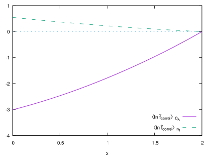
Figure 1: The corrections $\langle\ln\tilde{f}_{\rm correl}\rangle_{C_{A}}$ and $\langle\ln\tilde{f}_{\rm correl}\rangle_{n_{f}}$ as a function of $x$.

For $x=0$, $\langle\ln\tilde{f}_{\rm correl}\rangle_{C_{A}}$ and $\langle\ln\tilde{f}_{\rm correl}\rangle_{n_{f}}$ can be computed analytically, which gives

$$\langle\ln\tilde{f}_{\rm correl}\rangle_{C_{A}}=-\frac{11\zeta_{2}}{6}\,,\qquad\langle\ln\tilde{f}_{\rm correl}\rangle_{n_{f}}=\frac{\zeta_{2}}{3}\,.$$ (118)

4.5 Matching and issues with Sudakov shoulders for $FC_{x}$

It is interesting to study the matching to fixed order for the moments of energy energy correlation (93). Such observables feature a Sudakov shoulder Catani:1997xc , whose position can get dangerously close to the Sudakov peak for certain values of $x$. To examine this feature we now match the resummed NNLL distributions to NLO fixed-order differential cross sections obtained with EVENT2 Catani:1996vz . Although we only analyse $FC_{x}$ below, the procedure discussed in the following applies to all observables considered in this article. The matching is performed according to the log-R scheme (see for instance Catani:1992ua ; Monni:2011gb ). As it is customary in resummed calculations, to probe the size of subleading logarithmic terms we introduce a rescaling constant $x_{V}$ as

$$\ln\frac{1}{v}=\ln\frac{x_{V}}{v}-\ln x_{V}\,,$$ (119)

and expand the cross section around $\ln x_{V}/v$ neglecting subleading terms. Eventually we modify the resummed logarithm $\ln x_{V}/v$ in order to impose that the total cross section is reproduced at the kinematical endpoint $v_{\rm max}$

$$\ln\frac{x_{V}}{v}\rightarrow\frac{1}{p}\ln\left(1+\left(\frac{x_{V}}{v}\right)^{p}-\left(\frac{x_{V}}{v_{\rm max}}\right)^{p}\right)\,.$$ (120)

Here, $p$ denotes a positive number which controls how quickly the logarithms are switched off close to the endpoint. Since in the following we do not perform a phenomenological study, we simply set $p=1$ and $v_{\rm max}=1$ for the sake of simplicity.

To obtain our central predictions we set $\mu_{R}=Q$, with $Q$ being the centre-of-mass energy of the hard scattering, corresponding to $\alpha_{s}(M_{Z})=0.118$, and $x_{V}=1$. We then construct the uncertainty bands by varying $\mu_{R}$ and $x_{V}$ individually by a factor of two in either direction. The relevant formulae for the scale dependence are reported in the appendix of Ref. Banfi:2014sua .

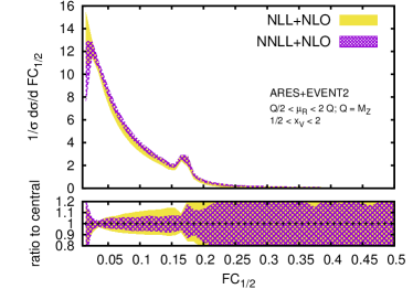
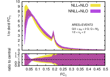
Figure 2: NNLL+NLO and NLL+NLO distributions for the two moments of EEC $FC_{1/2}$ and $FC_{1}$ at $Q=M_{Z}$. The lower inset shows the ratio to the relative central value for each of the two bands.

Figure 2 shows the NLO differential distribution matched to both NLL and NNLL for the cases $x=1/2$ and $x=1$. From the plots one can appreciate the following two interesting features.

The first is that the size of NNLL corrections increases with $x$. This can be explained by inspecting the parametrisation of the observable in the soft and collinear limit (96). The characteristic transverse momentum of the soft radiation is $k_{t}\sim Qv$, while the hard-collinear radiation occurs at scales $k_{t}\sim Qv^{\frac{1}{2-x}}$, with $x<2$. The soft scale is therefore lower than the collinear scales for $x<1$, the two coincide for $x=1$, and the situation is inverted for $2>x>1$. For a given value $v$ of the observable, the typical size of the soft logarithms (and hence of the soft corrections) does not depend on the moment parameter $x$. Conversely, the size of the hard-collinear logarithms increases with $x$, hence leading to larger subleading corrections. One also expects that corrections beyond NNLL become more sizeable as $x$ increases, as it is reflected by the scale uncertainty band in Figure 2. For $x>1$ the subleading corrections grow very large as the collinear scale becomes smaller than the soft one, which corresponds to a badly convergent logarithmic series. A consequence of this fact is that for $x>1$ the abscissa of the Landau pole moves towards larger values of $v$, and hence the differential distribution becomes non-perturbative at moderate values of $v$.

A second interesting observation is that the relative distance between the Sudakov peak and the shoulder decreases for increasing $x$. This implies that there is a value of $x$ for which the two overlap. Such a situation can be observed in the left plot of Figure 3 for $x=3/2$, where the curves are obtained at the $Z$ resonance and for central values of the scales.

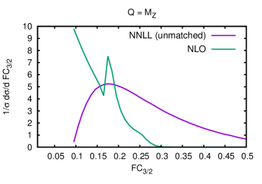
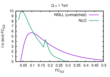
Figure 3: Comparison between the unmatched NNLL distribution with central scales and the NLO prediction for the moment of EEC $FC_{3/2}$ at $Q=M_{Z}$ (left) and $Q=1$ TeV (right).

In this case the solution provided by the resummation in the two-jet limit is obviously unphysical. The position of the Sudakov peak represents the bulk of the soft and collinear radiation probability in the two-jet configuration, and it coincides with the kinematic endpoint for the three-jet configuration, above which the distribution is again dominated by soft and collinear emissions.

This phenomenon is due to the violation of momentum conservation in the formulation of the resummed calculation, in which the exact kinematics in the presence of an extra hard parton is ignored. In such a situation one should perform a simultaneous resummation of the Sudakov logarithms treated here together with the logarithms that originate at the shoulder. This is currently out of reach at the logarithmic order analysed in this article.

While in this case a matching to fixed order results in an unphysical prediction, the right plot of Figure 3 shows that the situation improves at higher collider energies. As can be seen from this plot, for higher collider energies the position of the Sudakov peak moves towards smaller values of the observable, driven by the smaller coupling constant, while the position of the shoulder does note depend on $Q$. At these scales the resummed result is physical and can be matched to the fixed order. An example is reported in Figure 4, where the matched distribution for $Q=1$ TeV is shown.

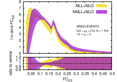
Figure 4: NNLL+NLO and NLL+NLO distributions for the moment of EEC $FC_{3/2}$ at $Q=1$ TeV. The lower inset shows the ratio to the relative central value.

5 Conclusions

In this paper we have completed the study of jet observables at NNLL accuracy in $e^{+}e^{-}$ annihilation, that started in refs. Banfi:2014sua ; Banfi:2016zlc . These results constitute the core of the ARES method for the semi-numerical resummation of jet observables at NNLL accuracy, which generalises the NLL procedure of refs. Banfi:2004yd ; Banfi:2003je ; Banfi:2001bz . This involves the calculation of an observable dependent Sudakov form factor, the radiator, which encodes the all-order cancellation of infrared singularities between real and virtual contributions, and that we have computed at NNLL accuracy for a generic rIRC safe observable.

As a byproduct, we have defined a generalisation of the well known CMW physical coupling in the soft limit, and given a closed expression for its relation to the $\overline{\rm MS}$ coupling up to ${\cal O}(\alpha_{s}^{3})$. This quantity is a universal ingredient for all resummations of rIRC safe observables, and as such it constitutes one of the main ingredients for a NNLL accurate parton shower algorithm.

As an application, we have computed NNLL resummed distributions for angularities and fractional moments of EEC, for all allowed values of the parameter $x$ they depend on. We have also presented a very basic phenomenology of moments of EEC, highlighting their main features. A particularly severe issue is that, for $x>1$, the Sudakov peak of the differential distribution, where the observable should be dominated by multiple soft-collinear emissions, becomes dangerously close to the edge of the phase space for real emissions, so that the core approximation underlying soft-collinear resummations breaks down. This situation is severe at LEP energies and prevents us to make any sense of resummed prediction matched to fixed order for certain values of $x>1$. This is not the case at a future $e^{+}e^{-}$ collider with centre-of-mass energy of $1\,\mathrm{TeV}$, where the Sudakov peak moves towards lower values of the observable, while the position of the kinematical boundary stays unchanged. This is a feature that should be considered when using these observables for phenomenology.

We stress that the procedure outlined in this paper is only an example on how to construct a Sudakov radiator. The same calculation could for instance be performed at all orders using the methods of Soft-Collinear Effective Theory (SCET), along the lines of what has been shown for thrust in Ref. Bauer:2018svx . To achieve a full resummation, the radiator should be supplemented by appropriate NLL and NNLL corrections due to the resolved real radiation. In this paper, we have defined the Sudakov radiator in such a way that all NLL, and most NNLL corrections are the same as in refs. Banfi:2014sua ; Banfi:2016zlc . The only exception is the NNLL correction $\delta\mathcal{F}_{\rm correl}$, which we had to redefine to ensure that the radiator could be computed analytically for a generic rIRC safe observable.

We also note that this very same radiator could in principle be used also for processes with incoming hadrons, for reactions with two hard emitting legs at the Born level. In that case, all corrections due to soft radiation, $\mathcal{F}_{\text{NLL}},\delta\mathcal{F}_{\rm sc},\delta\mathcal{F}_{\rm wa},\delta\mathcal{F}_{\rm correl}$ stay unchanged, and one has to evaluate parton distribution functions at the factorisation scales of order $v^{1/(a+b_{\ell})}Q$, and recompute only the hard-collinear contributions $C^{(1)}_{{\rm hc},\ell},\delta\mathcal{F}_{\rm hc},\delta\mathcal{F}_{\rm rec}$, as done for instance in Ref. Monni:2016ktx ; Bizon:2017rah for certain classes of observables. For processes with more than two legs, all terms in the master formula (2.2) must be redefined in order to account for the structure of the wide-angle soft radiation. This will be left for future work.

In summary, this work completes the formulation of a general method for to the calculation of any jet observable in processes with two legs, that can be systematically generalised to more complicated cases. We hope that the results presented here will define a solid starting point for future systematic studies of jet observables at all perturbative orders.

Appendix A Correlated two-parton emission

We start by decomposing the momenta of the two partons $k_{a}$ and $k_{b}$ as in Eq. (1). We then introduce relative variables to parameterise the two-parton phase space, as follows

$$\begin{split}&z^{(\ell)}_{a}=z\,z^{(\ell)}\,,\quad z_{b}^{(\ell)}=(1-z)\,z^{(\ell)}\,,\\ &\vec{q}_{a}=\frac{\vec{k}_{ta}}{z}\,,\quad\vec{q}_{b}=\frac{\vec{k}_{tb}}{1-z}\,,\end{split}$$ (121)

in terms of which the Lorentz invariant phase-space in $4-2\epsilon$ dimensions becomes

$$[dk_{a}][dk_{b}]=\frac{1}{(4\pi)^{2}}\frac{dz^{(\ell)}}{z^{(\ell)}}dz[z(1-z)]^{1-2\epsilon}\frac{d^{2-2\epsilon}q_{a}}{(2\pi)^{2-2\epsilon}}\frac{d^{2-2\epsilon}q_{b}}{(2\pi)^{2-2\epsilon}}\,.$$ (122)

Another useful change of variables is

$$\vec{k}_{t}=\vec{k}_{ta}+\vec{k}_{tb}\,,\qquad\vec{q}=\vec{q}_{a}-\vec{q}_{b}\,,$$ (123)

in terms of which the phase-space becomes

$$[dk_{a}][dk_{b}]=\frac{1}{(4\pi)^{2}}\frac{dz^{(\ell)}}{z^{(\ell)}}\frac{d^{2-2\epsilon}k_{t}}{(2\pi)^{2-2\epsilon}}dz[z(1-z)]^{1-2\epsilon}\frac{d^{2-2\epsilon}q}{(2\pi)^{2-2\epsilon}}=[dk]\frac{dz[z(1-z)]^{1-2\epsilon}}{4\pi}\frac{d^{2-2\epsilon}q}{(2\pi)^{2-2\epsilon}}\,,$$ (124)

where we have been able to factor out the phase space $[dk]$ defined in Eq. (12). Last, one can isolate the integration over $\phi$, the angle between $\vec{k}_{t}$ and $\vec{q}$, and introduce

$$m^{2}\equiv(k_{a}+k_{b})^{2}=z(1-z)q^{2}\,,$$ (125)

to obtain yet another expression for the two-body phase space

$$[dk_{a}][dk_{b}]=[dk]\frac{dz[z(1-z)]^{-\epsilon}}{(4\pi)^{2}}\frac{dm^{2}}{(m^{2})^{\epsilon}}\frac{d\Omega_{2-2\epsilon}}{(2\pi)^{1-2\epsilon}}\,.$$ (126)

The factor $d\Omega_{2-2\epsilon}$ is the azimuthal phase space for the vector $\vec{q}$ with respect to $\vec{k}_{t}$. Explicitly, this is given by

$$d\Omega_{2-2\epsilon}=\frac{(4\pi)^{\epsilon}}{\sqrt{\pi}\Gamma(\frac{1}{2}-\epsilon)}d\phi(\sin^{2}\phi)^{-\epsilon}\,.$$ (127)

where the relative angle $\phi$ in the range $0<\phi<\pi$.

In terms of these variables, the correlated matrix element $\tilde{M}_{s,0}^{2}(k_{a},k_{b})$ is given by

$$\tilde{M}_{s,0}^{2}(k_{a},k_{b})=(4\pi\alpha_{s}\mu_{R}^{2\epsilon})^{2}\frac{8C_{\ell}}{m^{2}(m^{2}+k_{t}^{2})}C_{ab}(k_{a},k_{b})\,,$$ (128)

where $\mu_{R}$ is the renormalisation scale, $C_{\ell}$ is the colour factor associated with the emitting leg, and

$$C_{ab}(k_{a},k_{b})=C_{A}(2\mathcal{S}+\mathcal{H}_{g})+n_{f}\mathcal{H}_{q}\,.$$ (129)

The contribution due to two final-state quarks in Eq. (129) has been multiplied by two, to compensate for the overall $1/2!$ factor in Eq. (85). The three functions $\mathcal{S}$, $\mathcal{H}_{g}$ and $\mathcal{H}_{q}$ are the $4-2\epsilon$-dimensional counterparts of the homonymous terms defined in Ref. Dokshitzer:1997iz . They depend only on the dimensionsless variables $z$, $\phi$ and $\mu^{2}\equiv m^{2}/k_{t}^{2}$. It is also useful to introduce the rescaled momenta $\vec{u}_{i}=\vec{q}_{i}/k_{t}$, such that

$$u_{a}^{2}=1+2\sqrt{\frac{1-z}{z}}\mu\cos\phi+\frac{1-z}{z}\mu^{2}\,,\qquad u_{b}^{2}=1-2\sqrt{\frac{z}{1-z}}\mu\cos\phi+\frac{z}{1-z}\mu^{2}\,.$$ (130)

In terms of these variables, we have

$$2\mathcal{S} =\frac{1}{z(1-z)}\left[\frac{1-(1-z)\mu^{2}/z}{u_{a}^{2}}+\frac{1-z\mu^{2}/(1-z)}{u_{b}^{2}}\right]$$ (131a)

$$\mathcal{H}_{g} =-4+(1-\epsilon)\frac{z(1-z)}{1+\mu^{2}}\left(2\cos\phi+\frac{(1-2z)\mu}{\sqrt{z(1-z)}}\right)^{2}$$

$$+\frac{1}{2(1-z)}\left[1-\frac{1-(1-z)\mu^{2}/z}{u_{a}^{2}}\right]+\frac{1}{2z}\left[1-\frac{1-z\mu^{2}/(1-z)}{u_{b}^{2}}\right]$$ (131b)

$$\mathcal{H}_{q} =1-\frac{z(1-z)}{1+\mu^{2}}\left(2\cos\phi+\frac{(1-2z)\mu}{\sqrt{z(1-z)}}\right)^{2}\,.$$ (131c)

Note that, in the limit $\mu^{2}\to 0$, one recovers the azimuthally unaveraged splitting functions, in particular

$$2\mathcal{S}+\mathcal{H}_{g}\to 2\left[\frac{1}{z(1-z)}-2+2(1-\epsilon)z(1-z)\cos^{2}\phi\right]\,,$$ (132a)

$$\mathcal{H}_{q}\to 1-4z(1-z)\cos^{2}\phi\,.$$ (132b)

References

- (1) C. Patrignani et al. [Particle Data Group], Chapter 9: Quantum Chromodynamics; Chin. Phys. C 40 (2016) no.10, 100001. doi:10.1088/1674-1137/40/10/100001
- (2) M. Dasgupta and G. P. Salam, Phys. Lett. B 512, 323 (2001) [hep-ph/0104277];
- (3) M. Dasgupta and G. P. Salam, JHEP 0203 (2002) 017 [hep-ph/0203009].
- (4) A. Banfi, G. Marchesini and G. Smye, JHEP 0208 (2002) 006 [hep-ph/0206076].
- (5) A. Gehrmann-De Ridder, T. Gehrmann, E. W. N. Glover and G. Heinrich, JHEP 0712 (2007) 094 [arXiv:0711.4711 [hep-ph]].
- (6) A. Gehrmann-De Ridder, T. Gehrmann, E. W. N. Glover and G. Heinrich, Phys. Rev. Lett. 100 (2008) 172001 [arXiv:0802.0813 [hep-ph]].
- (7) S. Weinzierl, Phys. Rev. Lett. 101 (2008) 162001 [arXiv:0807.3241 [hep-ph]].
- (8) S. Weinzierl, JHEP 0906 (2009) 041 [arXiv:0904.1077 [hep-ph]].
- (9) V. Del Duca, C. Duhr, A. Kardos, G. Somogyi, Z. Szor, Z. Trócsányi and Z. Tulipánt, Phys. Rev. D 94 (2016) no.7, 074019 doi:10.1103/PhysRevD.94.074019 [arXiv:1606.03453 [hep-ph]].
- (10) J. C. Collins, D. E. Soper and G. Sterman, Nucl. Phys. B 250 (1985) 199.
- (11) S. Catani, L. Trentadue, G. Turnock and B. R. Webber, Nucl. Phys. B 407, 3 (1993).
- (12) R. Bonciani, S. Catani, M. L. Mangano and P. Nason, Phys. Lett. B 575 (2003) 268 [hep-ph/0307035].
- (13) S. Catani, G. Turnock, B. R. Webber and L. Trentadue, Phys. Lett. B 263, 491 (1991).
- (14) S. Catani, G. Turnock and B. R. Webber, Phys. Lett. B 272, 368 (1991).
- (15) S. Catani and B. R. Webber, Phys. Lett. B 427, 377 (1998) [hep-ph/9801350].
- (16) Y. L. Dokshitzer, A. Lucenti, G. Marchesini and G. P. Salam, JHEP 9801 (1998) 011 [hep-ph/9801324].
- (17) A. J. Larkoski, D. Neill and J. Thaler, JHEP 1404 (2014) 017 doi:10.1007/JHEP04(2014)017 [arXiv:1401.2158 [hep-ph]].
- (18) A. Banfi, G. P. Salam and G. Zanderighi, JHEP 0503 (2005) 073 doi:10.1088/1126-6708/2005/03/073 [hep-ph/0407286].
- (19) A. Banfi, G. P. Salam and G. Zanderighi, Phys. Lett. B 584 (2004) 298 doi:10.1016/j.physletb.2004.01.048 [hep-ph/0304148].
- (20) A. Banfi, G. P. Salam and G. Zanderighi, JHEP 0201 (2002) 018 doi:10.1088/1126-6708/2002/01/018 [hep-ph/0112156].
- (21) A. Banfi, G. P. Salam and G. Zanderighi, JHEP 0408 (2004) 062 [hep-ph/0407287].
- (22) A. Banfi, G. P. Salam and G. Zanderighi, JHEP 1006 (2010) 038 doi:10.1007/JHEP06(2010)038 [arXiv:1001.4082 [hep-ph]].
- (23) T. Becher and M. D. Schwartz, JHEP 0807 (2008) 034 [arXiv:0803.0342 [hep-ph]].
- (24) R. Abbate, M. Fickinger, A. H. Hoang, V. Mateu and I. W. Stewart, Phys. Rev. D 83 (2011) 074021 doi:10.1103/PhysRevD.83.074021 [arXiv:1006.3080 [hep-ph]].
- (25) P. F. Monni, T. Gehrmann and G. Luisoni, JHEP 1108, 010 (2011) [arXiv:1105.4560 [hep-ph]].
- (26) Y. T. Chien and M. D. Schwartz, JHEP 1008 (2010) 058 [arXiv:1005.1644 [hep-ph]].
- (27) T. Becher and G. Bell, JHEP 1211 (2012) 126 [arXiv:1210.0580 [hep-ph]].
- (28) A. H. Hoang, D. W. Kolodrubetz, V. Mateu and I. W. Stewart, Phys. Rev. D 91 (2015) no.9, 094017 doi:10.1103/PhysRevD.91.094017 [arXiv:1411.6633 [hep-ph]].
- (29) D. de Florian and M. Grazzini, Nucl. Phys. B 704 (2005) 387 [hep-ph/0407241].
- (30) Z. Tulipánt, A. Kardos and G. Somogyi, Eur. Phys. J. C 77 (2017) no.11, 749 doi:10.1140/epjc/s10052-017-5320-9 [arXiv:1708.04093 [hep-ph]].
- (31) I. Moult and H. X. Zhu, arXiv:1801.02627 [hep-ph].
- (32) C. Frye, A. J. Larkoski, M. D. Schwartz and K. Yan, arXiv:1603.06375 [hep-ph].
- (33) M. Procura, W. J. Waalewijn and L. Zeune, arXiv:1806.10622 [hep-ph].
- (34) S. Moch, B. Ruijl, T. Ueda, J. A. M. Vermaseren and A. Vogt, Phys. Lett. B 782 (2018) 627 doi:10.1016/j.physletb.2018.06.017 [arXiv:1805.09638 [hep-ph]].
- (35) D. Kang, C. Lee and I. W. Stewart, Phys. Rev. D 88 (2013) 054004 [arXiv:1303.6952 [hep-ph]].
- (36) Z. B. Kang, X. Liu, S. Mantry and J. W. Qiu, Phys. Rev. D 88 (2013) 074020 [arXiv:1303.3063 [hep-ph]].
- (37) Z. B. Kang, X. Liu and S. Mantry, Phys. Rev. D 90 (2014) 1, 014041 [arXiv:1312.0301 [hep-ph]].
- (38) G. Bozzi, S. Catani, D. de Florian and M. Grazzini, Nucl. Phys. B 737 (2006) 73 [hep-ph/0508068].
- (39) T. Becher and M. Neubert, Eur. Phys. J. C 71 (2011) 1665 [arXiv:1007.4005 [hep-ph]].
- (40) A. Banfi, M. Dasgupta and S. Marzani, Phys. Lett. B 701 (2011) 75 [arXiv:1102.3594 [hep-ph]].
- (41) I. W. Stewart, F. J. Tackmann and W. J. Waalewijn, Phys. Rev. Lett. 106 (2011) 032001 [arXiv:1005.4060 [hep-ph]].
- (42) C. F. Berger, C. Marcantonini, I. W. Stewart, F. J. Tackmann and W. J. Waalewijn, JHEP 1104 (2011) 092 [arXiv:1012.4480 [hep-ph]].
- (43) T. Becher, X. Garcia i Tormo and J. Piclum, Phys. Rev. D 93 (2016) no.5, 054038 Erratum: [Phys. Rev. D 93 (2016) no.7, 079905] doi:10.1103/PhysRevD.93.054038, 10.1103/PhysRevD.93.079905 [arXiv:1512.00022 [hep-ph]].
- (44) T. Becher and M. Neubert, JHEP 1207 (2012) 108 [arXiv:1205.3806 [hep-ph]].
- (45) T. Becher, M. Neubert and L. Rothen, arXiv:1307.0025 [hep-ph].
- (46) A. Banfi, P. F. Monni, G. P. Salam and G. Zanderighi, Phys. Rev. Lett. 109 (2012) 202001 [arXiv:1206.4998 [hep-ph]].
- (47) I. W. Stewart, F. J. Tackmann, J. R. Walsh and S. Zuberi, arXiv:1307.1808 [hep-ph].
- (48) H. X. Zhu, C. S. Li, H. T. Li, D. Y. Shao and L. L. Yang, Phys. Rev. Lett. 110 (2013) 082001 [arXiv:1208.5774 [hep-ph]].
- (49) S. Catani, M. Grazzini and A. Torre, arXiv:1408.4564 [hep-ph].
- (50) T. T. Jouttenus, I. W. Stewart, F. J. Tackmann and W. J. Waalewijn, Phys. Rev. D 83 (2011) 114030 [arXiv:1102.4344 [hep-ph]].
- (51) W. Bizoń, P. F. Monni, E. Re, L. Rottoli and P. Torrielli, JHEP 1802 (2018) 108 doi:10.1007/JHEP02(2018)108 [arXiv:1705.09127 [hep-ph]].
- (52) X. Chen et al., arXiv:1805.00736 [hep-ph].
- (53) W. Bizoń et al., arXiv:1805.05916 [hep-ph].
- (54) A. Banfi, H. McAslan, P. F. Monni and G. Zanderighi, JHEP 1505 (2015) 102 [arXiv:1412.2126 [hep-ph]].
- (55) A. Banfi, H. McAslan, P. F. Monni and G. Zanderighi, Phys. Rev. Lett. 117 (2016) no.17, 172001 doi:10.1103/PhysRevLett.117.172001 [arXiv:1607.03111 [hep-ph]].
- (56) E. Laenen, G. F. Sterman and W. Vogelsang, Phys. Rev. D 63 (2001) 114018 doi:10.1103/PhysRevD.63.114018 [hep-ph/0010080].
- (57) L. J. Dixon, L. Magnea and G. F. Sterman, JHEP 0808 (2008) 022 doi:10.1088/1126-6708/2008/08/022 [arXiv:0805.3515 [hep-ph]].
- (58) J. Frenkel and J. C. Taylor, Nucl. Phys. B 246 (1984) 231.
- (59) J. G. M. Gatheral, Phys. Lett. B 133 (1983) 90.
- (60) S. Catani and M. Grazzini, Nucl. Phys. B 591 (2000) 435 doi:10.1016/S0550-3213(00)00572-1 [hep-ph/0007142].
- (61) S. Catani, B. R. Webber and G. Marchesini, Nucl. Phys. B 349 (1991) 635. doi:10.1016/0550-3213(91)90390-J
- (62) F. A. Berends and W. T. Giele, Nucl. Phys. B 313 (1989) 595. doi:10.1016/0550-3213(89)90398-2
- (63) Y. Li and H. X. Zhu, JHEP 1311 (2013) 080 doi:10.1007/JHEP11(2013)080 [arXiv:1309.4391 [hep-ph]].
- (64) Z. Nagy and D. E. Soper, JHEP 1206 (2012) 044 doi:10.1007/JHEP06(2012)044 [arXiv:1202.4496 [hep-ph]].
- (65) R. Á. Martínez, M. De Angelis, J. R. Forshaw, S. Plätzer and M. H. Seymour, arXiv:1802.08531 [hep-ph].
- (66) S. Jadach, A. Kusina, M. Skrzypek and M. Slawinska, Nucl. Phys. Proc. Suppl. 205-206 (2010) 295 doi:10.1016/j.nuclphysbps.2010.09.009 [arXiv:1007.2437 [hep-ph]].
- (67) H. T. Li and P. Skands, Phys. Lett. B 771 (2017) 59 doi:10.1016/j.physletb.2017.05.011 [arXiv:1611.00013 [hep-ph]].
- (68) S. Höche, F. Krauss and S. Prestel, JHEP 1710 (2017) 093 doi:10.1007/JHEP10(2017)093 [arXiv:1705.00982 [hep-ph]].
- (69) S. Höche and S. Prestel, Phys. Rev. D 96 (2017) no.7, 074017 doi:10.1103/PhysRevD.96.074017 [arXiv:1705.00742 [hep-ph]].
- (70) F. Dulat, S. Höche and S. Prestel, arXiv:1805.03757 [hep-ph].
- (71) M. Dasgupta, F. A. Dreyer, K. Hamilton, P. F. Monni and G. P. Salam, arXiv:1805.09327 [hep-ph].
- (72) C. F. Berger, T. Kucs and G. F. Sterman, Phys. Rev. D 68 (2003) 014012 doi:10.1103/PhysRevD.68.014012 [hep-ph/0303051].
- (73) A. J. Larkoski, G. P. Salam and J. Thaler, JHEP 1306 (2013) 108 doi:10.1007/JHEP06(2013)108 [arXiv:1305.0007 [hep-ph]].
- (74) S. Catani and B. R. Webber, JHEP 9710 (1997) 005 doi:10.1088/1126-6708/1997/10/005 [hep-ph/9710333].
- (75) S. Catani and M. H. Seymour, Nucl. Phys. B 485 (1997) 291 Erratum: [Nucl. Phys. B 510 (1998) 503] doi:10.1016/S0550-3213(96)00589-5, 10.1016/S0550-3213(98)81022-5 [hep-ph/9605323].
- (76) S. Catani, L. Trentadue, G. Turnock and B. R. Webber, Nucl. Phys. B 407 (1993) 3. doi:10.1016/0550-3213(93)90271-P
- (77) C. W. Bauer and P. F. Monni, arXiv:1803.07079 [hep-ph].
- (78) P. F. Monni, E. Re and P. Torrielli, Phys. Rev. Lett. 116, no. 24, 242001 (2016) doi:10.1103/PhysRevLett.116.242001 [arXiv:1604.02191 [hep-ph]].
- (79) Y. L. Dokshitzer, A. Lucenti, G. Marchesini and G. P. Salam, Nucl. Phys. B 511 (1998) 396 Erratum: [Nucl. Phys. B 593 (2001) 729] doi:10.1016/S0550-3213(97)00650-0, 10.1016/S0550-3213(00)00646-5 [hep-ph/9707532].