Scale-Invariant Continuous Entanglement Renormalization of a Chern Insulator

Abstract

The multi-scale entanglement renormalization ansatz (MERA) postulates the existence of quantum circuits that renormalize entanglement in real space at different length scales. Chern insulators, however, cannot have scale-invariant discrete MERA circuits with finite bond dimension. In this Letter, we show that the continuous MERA (cMERA), a modified version of MERA adapted for field theories, possesses a fixed point wavefunction with nonzero Chern number. Additionally, it is well known that reversed MERA circuits can be used to prepare quantum states efficiently in time that scales logarithmically with the size of the system. However, state preparation via MERA typically requires the advent of a full-fledged universal quantum computer. In this Letter, we demonstrate that our cMERA circuit can potentially be realized in existing analog quantum computers, i.e., an ultracold atomic Fermi gas in an optical lattice with light-induced spin-orbit coupling.

A quantum many-body system has a Hilbert space whose dimension grows exponentially with system size, making exact diagonalization of its Hamiltonian impractical. Fortunately, tensor networks Orús (2014); Bridgeman and Chubb (2017) are capable of efficiently representing the ground states of many systems with local interactions Vidal (2008); Verstraete and Cirac (2006); Verstraete et al. (2006); Hastings (2007); Vidal (2007); Wolf et al. (2008). Another powerful tool in many-body physics is the renormalization group (RG) Wilson (1974, 1975), which uses the fact that the description of a physical system can vary at different length scales, forming a hierarchical structure. The RG provides a systematic prescription to transform an exact microscopic description to an effective coarse-grained description. Applications of RG range from critical phenomena in condensed matter to the electroweak interaction in high-energy physics Zinn-Justin (2007).

One approach which combines tensor networks and renormalization group is called the multi-scale entanglement renormalization ansatz (MERA) Vidal (2008, 2007). MERA proposes a quantum circuit acting on a state which is initially entangled at many length scales. The two elementary building-block tensors of the MERA, isometries and disentanglers, are discrete unitary gates which physically implement RG in real space by successively removing entanglement at progressively larger length scales. Interestingly, since the circuit depth only increases logarithmically with the system size, a reversed MERA circuit can efficiently prepare a state with finer entanglement structure from a weakly-entangled initial state. In practice, MERAs are most convenient when the disentanglers and isometries are independent of the length scale Aguado and Vidal (2008); Pfeifer et al. (2009); König et al. (2009); König and Bilgin (2010); Singh and Vidal (2013); Evenbly and White (2016); Haegeman et al. (2018). The state that is left unchanged in the thermodynamic limit by these scale-invariant unitaries is termed a fixed-point wavefunction.

Experimentally, a reversed MERA circuit might be used to prepare exotic states, such as chiral topological states, which include integer quantum Hall states and certain fractional quantum Hall states Hansson et al. (2017); Wen (2017). Some fractional quantum Hall systems are believed to feature anyons useful for topological quantum computation Nayak et al. (2008). Due to their great theoretical interest, it would be useful to be able to study these systems under highly controlled settings, such as in ultracold atomic gases. However, to create a chiral topological state in the lab, we must not only engineer the parent Hamiltonian, but also cool the system down to the ground state. The latter is usually hard experimentally for topological states due to their long-range entanglement Bravyi et al. (2006). A reversed MERA circuit can possibly resolve this issue by directly generating the target chiral topological state from another state that is easier to obtain by cooling.

Here, as a first step towards finding a MERA for a fractional quantum Hall state, we instead search for a MERA whose fixed-point wavefunction describes an (integer) Chern insulator. A Chern insulator is an integer quantum Hall state on a lattice and is therefore a simpler system than the fractional quantum Hall state. However, there are no-go theorems stating that a MERA cannot have a Chern insulator ground state as its fixed-point wavefunction Barthel et al. (2010); Dubail and Read (2015); Wahl et al. (2013); Li and Mong (2017). Since conventional MERA only contains strictly local interactions, adding quasi-local interactions with quickly decaying tails could possibly circumvent the no-go theorems. A modified formalism of MERA adapted for field theories called continuous MERA (cMERA) Haegeman et al. (2013) can include such quasi-local interactions Hu and Vidal (2017). In contrast to the MERA paradigm, in which the renormalization circuit consists of discrete unitary gates, cMERA treats the circuit time, which corresponds to the length scale, as a continuous variable and generates continuous entanglement renormalization using a Hermitian Hamiltonian.

In this Letter, we show that a type of Chern insulator wavefunction can be generated by a scale-invariant cMERA circuit. The Chern insulator model we consider is the Bernevig-Hughes-Zhang model in the continuum limit Bernevig et al. (2006). In addition, we propose a possible experimental realization of the cMERA circuit with neutral ${}^{171}\mathrm{Yb}$ atoms in an optical lattice by introducing spin-orbit coupling.

Our work complements and can be contrasted with Refs. Wen et al. (2016); Swingle and McGreevy (2016). While Ref. Wen et al. (2016) previously developed a cMERA for the continuous Chern insulator model mentioned above, our work uses a scale-invariant disentangler. Other prior work in Ref. Swingle and McGreevy (2016) presented a scale-invariant entanglement renormalization for a two-band Chern insulator model. While Ref. Swingle and McGreevy (2016) makes use of the lattice structure and quasi-adiabatic paths between a series of gapped Hamiltonians, our cMERA approach allows smooth time evolution and emphasizes the continuum physics. Another difference is that the RG evolution in Ref. Swingle and McGreevy (2016) involves interactions decaying with distance faster than any power-law function but slower than an exponential, whereas our cMERA only needs an exponentially decaying interaction. Other known methods for representing chiral topological states include artificial neural network quantum states Huang and Moore (2017); Kaubruegger et al. (2018); Glasser et al. (2018), projected entangled pair states Wahl et al. (2013, 2014); Poilblanc et al. (2015, 2016), matrix product states Zaletel and Mong (2012), and polynomial-depth unitary circuits Schmoll and Orús (2017).

Review of cMERA.—Within the framework of conventional MERA Vidal (2008, 2007), disentanglers $V_{u}$ and isometries $W_{u}$ are strictly local discrete unitary operators employed to renormalize entanglement at layer $u\in\mathbb{Z}^{+}$. In cMERA Haegeman et al. (2013), we simply replace them by continuous unitary transformations, which are infinitesimally generated by self-adjoint operators $K(u)$ and $L$: $V_{u}\rightarrow e^{-iK(u)\text{d}u}$, $W_{u}\rightarrow e^{-iL\text{d}u}$. The notation $\text{d}u$ denotes an infinitesimal RG step, and $u\in(-\infty,0]$. When the continuous variable $u$ approaches zero, the system is said to be at the ultraviolet (UV) length scale, possessing both short-range and long-range entanglement. As $u\rightarrow-\infty$, the system flows to the infrared (IR) length scale, where short-range entanglement is removed and nearly all degrees of freedom are disentangled from each other. Note that the generator of disentangler $K(u)$ can in general depend on scale $u$. A cMERA is called scale-invariant if $K(u)$ is independent of $u$.

To emulate the coarse-graining behavior of isometries in conventional lattice MERA, $L$ is chosen to be the scaling transformation in field theory. For example, for a single fermion field $\psi(\mathbf{x})$ in $d$ spatial dimensions, we pick $L=-\frac{i}{2}\int\left(\psi^{\dagger}(\mathbf{x})\,\mathbf{x}\cdot\nabla\psi(\mathbf{x})-\mathbf{x}\cdot\nabla\psi^{\dagger}(\mathbf{x})\,\psi(\mathbf{x})\right)\mathrm{d}^{d}\mathbf{x}$ Haegeman et al. (2013); Wen et al. (2016); thereby, fermionic operators $\psi(\mathbf{x})$ in real space and $\psi(\mathbf{k})$ in momentum space satisfy the following scaling transformations: $e^{-iuL}\psi(\mathbf{x})e^{iuL}=e^{\frac{d}{2}u}\psi(e^{u}\mathbf{x})$, $e^{-iuL}\psi(\mathbf{k})e^{iuL}=e^{-\frac{d}{2}u}\psi(e^{-u}\mathbf{k})$. One can check that the anti-commutation relations $\{\psi(\mathbf{x}),\psi^{\dagger}(\mathbf{x}^{\prime})\}=\delta(\mathbf{x}-\mathbf{x}^{\prime})$ in real space and $\{\psi(\mathbf{k}),\psi^{\dagger}(\mathbf{k}^{\prime})\}=\delta(\mathbf{k}-\mathbf{k}^{\prime})$ in momentum space are preserved under the scaling transformation. We will sometimes abuse the terminology to call $K(u)$ and $L$ themselves the disentangler and the isometry rather than the verbose generator of disentangler and generator of isometry.

The renormalized wavefunction is governed by the Schrödinger equation,

$$i\frac{\partial}{\partial u}|{\Psi^{S}(u)}\rangle=[K(u)+L]|{\Psi^{S}(u)}\rangle,$$ (1)

where the superscript $S$ denotes the Schrödinger picture. In this Letter, we will focus on the interaction picture which provides a more convenient way to look at continuous entanglement renormalization. We treat $L$ as a “free” Hamiltonian and $K(u)$ as an “interaction” Hamiltonian, i.e., $|{\Psi^{I}(u)}\rangle=e^{iuL}|{\Psi^{S}(u)}\rangle$, where the superscript $I$ denotes the interaction picture. Substituting this equation into Eq. (1), we obtain

$$i\frac{\partial}{\partial u}|{\Psi^{I}(u)}\rangle=\hat{K}(u)|{\Psi^{I}(u)}\rangle,$$ (2)

where $\hat{K}(u)\overset{\mathrm{{def}}}{=}e^{iuL}K(u)e^{-iuL}$ is the disentangler in the interaction picture. The renormalized wavefunction $|{\Psi^{I}(u)}\rangle$ at scale $u$ can be formally written in terms of the IR state $|{\Omega_{\mathrm{IR}}^{I}}\rangle\equiv|{\Psi^{I}(u\rightarrow-\infty)}\rangle$ as

$$|{\Psi^{I}(u)}\rangle=\mathcal{P}\exp\left(-i\int_{-\infty}^{u}\hat{K}(u^{\prime})\mathrm{d}u^{\prime}\right)|{\Omega_{\mathrm{IR}}^{I}}\rangle,$$ (3)

where $\mathcal{P}$ is the path ordering operator. Unless otherwise stated, we will only consider the interaction picture; therefore, we will drop the superscript $I$ in the rest of this Letter.

A continuous Chern insulator model.—We begin with a two-band continuous Chern insulator model in two spatial dimensions Bernevig et al. (2006) with Hamiltonian $H=\int\mathrm{d}^{2}\mathbf{k}\,\psi^{\dagger}(\mathbb{\mathbf{k}})[\mathbf{R}(\mathbf{k})\cdot\boldsymbol{\sigma}]\psi(\mathbf{k}),$ where $\mathbf{k}=(k_{x},\>k_{y})\in\mathbb{R}^{2}$, $\mathbf{R}(\mathbf{k})=(k_{x},\>k_{y},\>m-k^{2}),\>m>0,\>k\equiv|\mathbf{k}|=\sqrt{k_{x}^{2}+k_{y}^{2}}$, and $\boldsymbol{\sigma}=(\sigma_{x},\>\sigma_{y},\>\sigma_{z})$ is a vector of Pauli matrices. The fermionic operator $\psi(\mathbf{k})$ is a two-component spinor $\psi(\mathbf{k})\equiv\left(\begin{array}[]{cc}\psi_{1}(\mathbf{k})&\psi_{2}(\mathbf{k})\end{array}\right)^{T}$ whose components satisfy $\{\psi_{i}^{\dagger}(\mathbf{k}),\psi_{j}(\mathbf{k}^{\prime})\}=\delta_{ij}\,\delta(\mathbf{k}-\mathbf{k}^{\prime})$ for $i,j\in\left\{1,2\right\}$.

The ground state, which has the lower band filled, is Wen et al. (2016)

$$|{\Psi}\rangle =\prod_{\mathbf{k}}\left(u_{\mathbf{k}}\psi_{2}^{\dagger}(\mathbf{k})-v_{\mathbf{k}}\psi_{1}^{\dagger}(\mathbf{k})\right)|{\mathrm{vac}}\rangle,$$ (4)

$$u_{\mathbf{k}} =\frac{1}{\sqrt{N_{k}}}\left(\left(m-k^{2}\right)+\sqrt{(m-k^{2})^{2}+k^{2}}\right),$$

$$v_{\mathbf{k}} =\frac{1}{\sqrt{N_{k}}}\left(ke^{-i\theta_{k}}\right),$$

where $N_{k}$ is a $k$-dependent normalization factor such that $|u_{\mathbf{k}}|^{2}+|v_{\mathbf{k}}|^{2}=1$, and the state $|{\mathrm{vac}}\rangle$ is the vacuum state annihilated by $\psi_{1,2}(\mathbf{k})$. The angle $\theta_{k}$ is defined via $k_{x}=k\cos\theta_{k}$ and $k_{y}=k\sin\theta_{k}$, i.e., it is the polar angle in momentum space. The Chern number of the bottom band of this two-band system is $C=\frac{1}{4\pi}\int_{\mathbb{R}^{2}}\mathrm{d}^{2}\mathbf{k}\>\mathbf{\mathbf{n}}(\mathbf{k})\cdot\left(\frac{\partial\mathbf{n}(\mathbf{k})}{\partial k_{x}}\times\frac{\partial\mathbf{n}(\mathbf{k})}{\partial k_{y}}\right)=1$, where $\mathbf{n}(\mathbb{\mathbf{k}})\equiv\frac{\mathbf{R}(\mathbf{k})}{|\mathbf{R}(\mathbf{k})|}$ and where the integrand divided by two is called the Berry curvature.

Now, we show how to obtain a scale-invariant cMERA for this model.

Entanglement renormalization of the Chern insulator.—Following the convention in Refs. Nozaki et al. (2012); Haegeman et al. (2013); Wen et al. (2016), we take the Gaussian ansatz for the disentangler in the Schrödinger picture, $K(u)=i\int\mathrm{d}^{2}\mathbf{k}\Big{[}g(\mathbf{k},u)\psi_{1}^{\dagger}(\mathbf{k})\psi_{2}(\mathbf{k})+g^{*}(\mathbf{k},u)\psi_{1}(\mathbf{k})\psi_{2}^{\dagger}(\mathbf{k})\Big{]}$ . If we require our disentangler to be scale-invariant, then $g(\mathbf{k},u)$ should not have explicit $u$ dependence, $g(\mathbf{k},u)=g(\mathbf{k})$. We also take the ansatz that $g(\mathbf{k})=\mathcal{H}(k)e^{-i\theta_{k}}$, where $\mathcal{H}(k)$ is a real-valued function to be determined. Through rewriting the disentangler as $K(u)=\int\mathrm{d}^{2}\mathbf{k}\,\psi^{\dagger}(\mathbf{k})[\mathbf{H}(\mathbf{k})\cdot\boldsymbol{\sigma}]\psi(\mathbf{k})$ with $\mathbf{H}(\mathbf{k})=(\mathcal{H}(k)\sin\theta_{k},-\mathcal{H}(k)\cos\theta_{k},0)$, we can intuitively understand its action by imagining an effective magnetic field of strength $\mathcal{H}(k)$ in a clockwise direction about the origin applied to the pseudo-spin at each momentum point. In the interaction picture, the disentangler becomes

$$\hat{K}(u)=i\int\mathrm{d}^{2}\mathbf{k} \biggl{[}\mathcal{H}(e^{-u}k)e^{-i\theta_{k}}\psi_{1}^{\dagger}(\mathbf{k})\psi_{2}(\mathbf{k})$$

$$+\mathcal{H}(e^{-u}k)e^{i\theta_{k}}\psi_{1}(\mathbf{k})\psi_{2}^{\dagger}(\mathbf{k})\biggr{]}.$$ (5)

Now, we start to renormalize the wavefunction and determine the form of the disentangler. We assume that the renormalized wavefunction at scale $u$ can be expressed as

$$|{\Psi(u)}\rangle=\prod_{\mathbf{k}}(P_{\mathbf{k}}(u)\psi_{2}^{\dagger}(\mathbf{k})-Q_{\mathbf{k}}(u)\psi_{1}^{\dagger}(\mathbf{k}))|{\mathrm{vac}}\rangle,$$ (6)

with $\left|P_{\mathbf{k}}(u)\right|^{2}+\left|Q_{\mathbf{k}}(u)\right|^{2}=1$. From Eq. (2), we get

$$P_{\mathbf{k}}(u) =A_{\mathbf{k}}e^{-i\varphi(e^{-u}\mathbf{k})}+B_{\mathbf{k}}e^{i\varphi(e^{-u}\mathbf{k})},$$ (7)

$$Q_{\mathbf{k}}(u) =-ie^{-i\theta_{k}}\left[A_{\mathbf{k}}e^{-i\varphi(e^{-u}\mathbf{k})}-B_{\mathbf{k}}e^{i\varphi(e^{-u}\mathbf{k})}\right].$$

Coefficients $A_{\mathbf{k}}$ and $B_{\mathbf{k}}$ are complex numbers with $|A_{\mathbf{k}}|^{2}+|B_{\mathbf{k}}|^{2}=\frac{1}{2}$, and $\varphi(e^{-u}\mathbf{k})\equiv\int_{ke^{-u}}^{\infty}\mathcal{H}\left(t\right)\frac{\mathrm{d}t}{t}$. At UV scale $u=0$, the wavefunction should match the ground state in Eq. (4); at IR scale $u\to-\infty$, we would like the renormalized wavefunction to be the product state $\prod_{\mathbf{k}}\psi_{1}^{\dagger}(\mathbf{k})|{\mathrm{vac}}\rangle$ or the product state $\prod_{\mathbf{k}}\psi_{2}^{\dagger}(\mathbf{k})|{\mathrm{vac}}\rangle$ Nozaki et al. (2012); Haegeman et al. (2013); Wen et al. (2016). By taking $A_{\mathbf{k}}=-\frac{1}{2i}$ and $B_{\mathbf{k}}=\frac{1}{2i}$, the boundary conditions can be satisfied by requiring

$$\mathcal{\mathcal{H}}\left(k\right)=\frac{k(m+k^{2})}{2\left[k^{4}+k^{2}(1-2m)+m^{2}\right]}.$$ (8)

Substituting Eq. (8) into Eqs. (6) and (7), we attain an explicit form of the renormalized wavefunction,

$$|{\Psi(u)}\rangle= \prod_{\mathbf{k}}\frac{1}{\sqrt{N_{k,u}}}\times$$

$$\bigg{[}\Big{(}(m-k^{2}e^{-2u}) +\sqrt{(m-k^{2}e^{-2u})^{2}+k^{2}e^{-2u}}\Big{)}\>\psi_{2}^{\dagger}(\mathbf{k})$$

$$-k\,e^{-u}e^{-i\theta_{k}}\> \psi_{1}^{\dagger}(\mathbf{k})\bigg{]}|{\mathrm{vac}}\rangle,$$ (9)

where $N_{k,u}$ is a normalization factor that depends on $k$ and $u$. The Berry curvature of the renormalized wavefunction at different $u$ is shown schematically in FIG. 1. The IR state is $|{\Omega_{\mathrm{IR}}}\rangle=\lim_{u\rightarrow-\infty}|{\Psi(u)}\rangle=\prod_{\mathbf{k}}e^{-i\theta_{k}}\psi_{1}^{\dagger}(\mathbf{k})|{\mathrm{vac}}\rangle$, which is equal to $\prod_{\mathbf{k}}\psi_{1}^{\dagger}(\mathbf{k})|{\mathrm{vac}}\rangle=\prod_{\mathbf{x}}\psi_{1}^{\dagger}(\mathbf{x})|{\mathrm{vac}}\rangle$ up to an overall phase. Note that the nonzero Chern number does not survive in the IR state because the integration operation does not commute with the limit $u\rightarrow-\infty$. However, at any finite $u$, the Chern number is always one. Therefore, there is no phase transition during the entanglement renormalization process, consistent with the result in Ref. Wen et al. (2016).

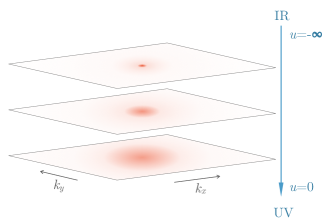
Figure 1: Berry curvature of the renormalized wavefunction in the interaction picture at different scales $u$, drawn schematically in momentum space. The blue arrow corresponds to the direction of the reversed cMERA circuit. The area contributing to the Chern number expands as one approaches the UV scale.

To analyze the spatial structure of the disentangler, we rewrite the expression for $\mathcal{\mathcal{H}}\left(k\right)$. We first define $\lambda_{+}$ and $\lambda_{-}$ as the two roots of the equation $x^{2}+(1-2m)x+m^{2}=0$, $\lambda_{\pm}=\frac{-1+2m\pm\sqrt{1-4m}}{2}$. They are real and negative when $0<m<1/4$. Although setting this restriction on $m$ is not necessary for our disentangler, we will assume it in the following in order to assist our experimental realization. Now, the expression $\mathcal{\mathcal{H}}\left(k\right)$ can be rewritten as

$$\mathcal{\mathcal{H}}\left(k\right)= \left(\frac{-1+\sqrt{1-4m}}{4\sqrt{1-4m}}\right)\frac{k}{k^{2}-\lambda_{+}}$$

$$+\left(\frac{1+\sqrt{1-4m}}{4\sqrt{1-4m}}\right)\frac{k}{k^{2}-\lambda_{-}}.$$ (10)

By inserting this expression into Eq. (5) and performing a Fourier transform, it can be shown that the disentangler in real space decays exponentially with characteristic length $e^{-u}\mathrm{max}\{\sqrt{-\lambda_{+}},\,\sqrt{-\lambda_{-}}\}$. Therefore, our cMERA involves quasi-local interactions.

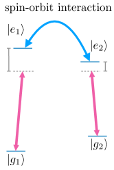
Figure 2: A scheme to engineer the cMERA circuit in the interaction picture. The two excited states are coupled by spin-orbit interaction to each other and by off-resonant lasers to the two ground states.

Experimental realization of the cMERA circuit.—We propose a way to realize our reversed cMERA circuit to prepare a Chern insulator state in an optical lattice with neutral ${}^{171}\mathrm{Yb}$, which are fermionic atoms with two outer electrons. From now on, we will drop the word “reversed” for our cMERA circuit when the context is clear. Recall that the cMERA circuit starts with an initial IR state. As discussed above, the IR state at $u\rightarrow-\infty$ does not have the correct Chern number; therefore, we start from a near-IR state with large negative $u$. In addition, the cMERA circuit is only valid on a lattice when the continuum approximation holds. Therefore, throughout the circuit, the physical length scale $e^{-u}\mathrm{max}\{\sqrt{-\lambda_{+}},\sqrt{-\lambda_{-}}\}$ should be significantly larger than the lattice spacing, but significantly smaller than the total size of the lattice. Going forward, we begin with a near-IR state and use our cMERA circuit to obtain the UV state without ever violating the requirements of the continuum approximation.

Here, we assume that we already have an initial near-IR state waiting to be inserted into the cMERA circuit. Since, in finite-size systems, the Berry curvature is concentrated on a few discrete momentum points near $k=0$, the preparation of this near-IR state should be fast if we can individually create states at each point in momentum space. In the Supplemental Material, we provide one possible method for generating this initial state.

We now present the cMERA circuit engineering scheme (see Supplemental Material for details). We use $|{g_{1}}\rangle$ and $|{g_{2}}\rangle$ as shorthand notations for the two stable hyperfine ground states $|{F=1/2,\>m_{F}=-1/2}\rangle$ and $|{F=1/2,\>m_{F}=1/2}\rangle$ in ${}^{1}\mathrm{S}_{0}$; these form the basis of our spinor $\psi(\mathbf{k})\equiv\left(\begin{array}[]{cc}\psi_{1}(\mathbf{k})&\psi_{2}(\mathbf{k})\end{array}\right)^{T}$. We find that if we have two metastable excited states $|{e_{1}}\rangle$ and $|{e_{2}}\rangle$ (e.g. from the ³P manifold) with quadratic dispersions coupled by spin-orbit interaction and couple them off-resonantly to the respective ground states as shown in FIG. 2, then the disentangler in the interaction picture can be engineered. Intuitively, the spin-orbit interaction allows us to generate a momentum-dependent effective magnetic field for Eq. (5), whereas the off-resonant couplings to quadratic dispersive bands induce quadratic terms in the denominators of Eq. (10). To accomplish this, we utilize the scheme detailed in Refs. Campbell et al. (2011); Campbell and Spielman (2016); Huang et al. (2016); Galitski and Spielman (2013) to create two dressed excited states coupled by spin-orbit interaction. However, as the two dressed states are linear combinations of bare excited states, the dressed states do not have good quantum numbers to have clear selection rules to forbid the transitions $|{g_{1}}\rangle\longleftrightarrow|{e_{2}}\rangle$ and $|{g_{2}}\rangle\longleftrightarrow|{e_{1}}\rangle$. Nevertheless, by carefully choosing the driving fields to couple ground states to the bare excited states, we can create interferences to generate synthetic selection rules. By varying the laser parameters as the circuit progresses, we can engineer the disentangler in the interaction picture.

When the UV state is generated by the cMERA circuit, one can then use the experimental techniques introduced in Refs. Hauke et al. (2014); Alba et al. (2011); Fläschner et al. (2016) to measure the Chern number and the Berry curvature.

Discussion.—In this work, we found a quasi-local cMERA whose fixed-point wavefunction is a Chern insulator. This is a novel and unexpected way to represent systems with chiral topological order. We also demonstrate that our quasi-local quantum circuit can be realized experimentally in a cold atom system, despite the common intuition that a quantum circuit should be strictly local to allow easier implementation.

In our realization, we only explored one possibility to engineer spin-orbit coupling, but it may be possible to engineer the interaction in other ways, such as using magnetic fields on a chip Anderson et al. (2013) or microwaves Grusdt et al. (2017). Other alkaline-earth atoms could also provide promising experimental platforms. Although our experimental realization took place in the interaction picture, one could in principle use the Schrödinger picture for cMERA, where the lattice constant must continuously contract Huckans et al. (2009); Al-Assam et al. (2010).

It is also interesting that the Chern insulator ground state is a fixed point of our cMERA with finite correlation length. This observation seems to contradict the usual intuition that the fixed point correlation length must be zero or infinity, as the correlation length must decrease under rescaling of each strictly local RG step in real space. However, since our cMERA involves continuous time evolution and quasi-local interactions, it has potential to restore the original correlation length after a finite time evolution. The no-go theorems in Refs. Barthel et al. (2010); Dubail and Read (2015); Wahl et al. (2013); Li and Mong (2017) are similarly circumvented by a cMERA construction. Our work suggests that quasi-local RG transformations are a more powerful framework than strictly local RG transformations. It also might shed light on some of the key properties of MERA-like formalisms for a wide range of chiral topological states. In the future, we hope to extend the methods of this Letter to fractional quantum Hall states.

Supplemental Material

In this Supplemental Material, we provide details on the experimental realization. In Section I, we show how to engineer a synthetic selection rule between dressed states in the absence of any good quantum number. With that technique in mind, we show a scheme to realize the cMERA circuit in Section II. After that, in Section III, we provide one way to prepare the initial state for the cMERA circuit by using spatial light modulators Fukuhara et al. (2013); Nogrette et al. (2014).

I Synthetic Selection Rules

In this section, we introduce a trick that will be useful for engineering the disentangler in a real atomic system. Suppose that we have a three-level system composed of states $|{s_{1}}\rangle$, $|{s_{2}}\rangle$, and $|{g}\rangle$. In the presence of an on-resonance driving with Rabi frequency $\Omega$ between bare states $|{s_{1}}\rangle$ and $|{s_{2}}\rangle$, two dressed states $|{d_{1}}\rangle$ and $|{d_{2}}\rangle$ are formed. We are going to show that by fine-tuning the Rabi frequencies $\chi_{1}$ and $\chi_{2}$, we can generate a synthetic selection rule from state $|{g}\rangle$ to the two dressed states $|{d_{1}}\rangle$ and $|{d_{2}}\rangle$, e.g., $|{g}\rangle\rightarrow|{d_{2}}\rangle$ is allowed while $|{g}\rangle\rightarrow|{d_{1}}\rangle$ is forbidden. (Once we prove this, the converse case where $|{g}\rangle\rightarrow|{d_{1}}\rangle$ is allowed and $|{g}\rangle\rightarrow|{d_{2}}\rangle$ is forbidden is a trivial generalization.) We consider a driving Hamiltonian, which under rotating wave approximation is

$$h=\left(\begin{array}[]{ccc}0&\chi_{1}^{*}e^{i(\omega_{1}-\Omega+\delta)t}&\chi_{2}^{*}e^{i(\omega_{2}-\Omega+\delta)t}\\ \chi_{1}e^{-i(\omega_{1}-\Omega+\delta)t}&\omega_{1}&\Omega e^{-i(\omega_{1}-\omega_{2})t}\\ \chi_{2}e^{-i(\omega_{2}-\Omega+\delta)t}&\Omega e^{i(\omega_{1}-\omega_{2})t}&\omega_{2}\end{array}\right).$$ (S1)

The order of the columns (rows) is $|{g}\rangle$, $|{s_{1}}\rangle$, $|{s_{2}}\rangle$. We have assumed that $|\omega_{1}-\omega_{2}|\gg\Omega$, allowing us to neglect some transitions that are far off-resonant. The level diagram is illustrated in FIG. S1.

Going to the rotating frame defined by the unitary matrix

$$U=\left(\begin{array}[]{ccc}1&0&0\\ 0&e^{-i(\omega_{1}-\omega_{2})t}&0\\ 0&0&1\end{array}\right),$$ (S2)

we obtain the effective Hamiltonian

$$U^{\dagger}hU-i\partial_{t}U^{\dagger}U=\left(\begin{array}[]{ccc}0&\chi_{1}^{*}e^{i(\omega_{2}-\Omega+\delta)t}&\chi_{2}^{*}e^{i(\omega_{2}-\Omega+\delta)t}\\ \chi_{1}e^{-i(\omega_{2}-\Omega+\delta)t}&\omega_{2}&\Omega\\ \chi_{2}e^{-i(\omega_{2}-\Omega+\delta)t}&\Omega&\omega_{2}\end{array}\right).$$ (S3)

After diagonalizing the $2\times 2$ block on the bottom right, we obtain the following Hamiltonian:

$$\left(\begin{array}[]{ccc}0&\frac{1}{\sqrt{2}}(\chi_{1}^{*}+\chi_{2}^{*})e^{i(\omega_{2}-\Omega+\delta)t}&\frac{1}{\sqrt{2}}(\chi_{1}^{*}-\chi_{2}^{*})e^{i(\omega_{2}-\Omega+\delta)t}\\ \frac{1}{\sqrt{2}}(\chi_{1}+\chi_{2})e^{-i(\omega_{2}-\Omega+\delta)t}&\omega_{2}+\Omega&0\\ \frac{1}{\sqrt{2}}(\chi_{1}-\chi_{2})e^{-i(\omega_{2}-\Omega+\delta)t}&0&\omega_{2}-\Omega\end{array}\right).$$ (S4)

We denote the dressed state with energy $\omega_{2}+\Omega$ as $|{d_{1}}\rangle$, and the dressed state with energy $\omega_{2}-\Omega$ as $|{d_{2}}\rangle$. We can see that if we fine-tune $\chi_{1}=-\chi_{2}$, we synthesize a selection rule where only the transition between $|{d_{2}}\rangle$ and $|{g}\rangle$ is allowed. The synthetic Rabi frequency is then $\sqrt{2}\chi_{1}$.

This synthetic selection rule can be understood by considering two separate rotating frames with respect to states $|{s_{1}}\rangle$ and $|{s_{2}}\rangle$, as shown in FIG. S1. In each rotating frame, we have dressed states $|{d_{1}}\rangle$ and $|{d_{2}}\rangle$. We can couple $|{g}\rangle$ to dressed states either by driving $|{g}\rangle$ to dressed states in the $|{s_{1}}\rangle$ rotating frame or in the $|{s_{2}}\rangle$ rotating frame. By creating interference between the two channels, we obtain a synthetic selection rule.

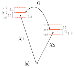
Figure S1: A toy model of synthetic selection rules. Bare states $|{s_{1}}\rangle$ and $|{s_{2}}\rangle$ are driven by a field with Rabi frequency $\Omega$, whereby two dressed states $|{d_{1}}\rangle$ and $|{d_{2}}\rangle$ are created. In view of the rotating frame, the dressed states are linear combinations of bare states. As a result, they do not have good quantum numbers to constitute a selection rule when coupling to another state, say $|{g}\rangle$. A synthetic selection rule can be generated through applying two driving fields from $|{g}\rangle$ to $|{s_{1}}\rangle$ and $|{s_{2}}\rangle$ with fine-tuned Rabi frequencies $\chi_{1}$ and $\chi_{2}$, respectively. For example, we can forbid the transition from $|{g}\rangle$ to $|{d_{1}}\rangle$ by choosing $\chi_{1}=-\chi_{2}$.

II The Continuous MERA Circuit Engineering

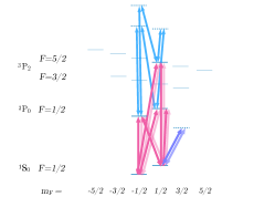
(a)(b)

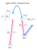
Figure S2: Disentangler engineering. (a) A magnetic field is applied to induce hyperfine splittings. The excited states are coupled by Raman beams (colored in blue) to generate an effective spin-orbit interaction. They are chosen from the hyperfine manifolds ${}^{3}\mathrm{P}_{2}$ $F=5/2$ and ${}^{3}\mathrm{P}_{0}$ $F=1/2$, which are long-lived to circumvent dissipation issues. Their ultra-narrow linewidths are on the order of tens of millihertz Zhang et al. (2015); Kohno et al. (2009); Lemke et al. (2009); Park et al. (2013); Yamaguchi (2008). Additionally, we also have two sets of multiple lasers, colored in light and dark pink, coupling the ground states to the excited states to engineer the disentangler of our cMERA by creating synthetic selection rules. (b) The effective couplings between ground states and the dressed excited states are generated from the scheme shown in (a). We ignore a third dressed state since it is far off-resonant. Now we effectively create two dressed excited states coupled by spin-orbit interaction, which are coupled to the ground states by two pairs of drivings colored in light and dark pink. The synthetic selection rules forbid $|{g_{1},\mathbf{k}}\rangle\longleftrightarrow|{e_{2},\mathbf{k}}\rangle$ and $|{g_{2},\mathbf{k}}\rangle\longleftrightarrow|{e_{1},\mathbf{k}}\rangle$. The effective Rabi frequencies and detunings for two pairs of effective drivings are labeled by unprimed and primed notation. The band structures are ignored in this picture, so by detunings we mean the detunings at $\mathbf{k}=0$. The light and dark purple arrows on the bottom right in (a) and (b) both represent lasers used to cancel unwanted AC Stark shifts by coupling the ground states to some negative curvature bands of some excited state, e.g., an unused excited state in the ${}^{3}\mathrm{P}_{2}$ $F=5/2$ hyperfine manifold.

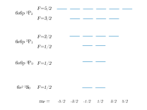
Figure S3: Energy level diagram of neutral atom ${}^{171}\mathrm{Yb}$. The hyperfine structure is shown. We employ the bottom two ground states as our spinor basis of the Chern insulator.

In this section, we show that by using the scheme shown in FIG. S2(b), we can engineer the disentangler in the interaction picture. Here, we choose the two hyperfine ground states of ${}^{171}\mathrm{Yb}$ shown in FIG. S3 as our spinor basis of the Chern insulator and effectively couple them to some dressed excited states by two pairs of driving fields. The meaning of “dressed” excited states will become clear shortly. Additionally, the dressed excited states are coupled by spin-orbit interaction, while transitions $|{g_{1},\mathbf{k}}\rangle\longleftrightarrow|{e_{2},\mathbf{k}}\rangle$ and $|{g_{2},\mathbf{k}}\rangle\longleftrightarrow|{e_{1},\mathbf{k}}\rangle$ are forbidden. In order to implement this idea in neutral ${}^{171}\mathrm{Yb}$ atoms, we need to use techniques introduced in Refs. Campbell et al. (2011); Campbell and Spielman (2016) and Section I. To create states coupled by spin-orbit coupling, we will utilize the method discussed in Refs. Campbell et al. (2011); Campbell and Spielman (2016). However, the dressed states created by that scheme do not have good quantum numbers to enforce selection rules. Therefore, we use the technique outlined in Section I to create a synthetic selection rule. In this part of the Supplemental Material, we show how to combine those techniques consistently in neutral ${}^{171}\mathrm{Yb}$.

First, we show how FIG. S2(b) arises from FIG. S2(a), inducing the disentangler interaction. We first consider the case with the set of lasers colored in dark pink in FIG. S2(a) with additional Raman lasers coupling the bare excited states. This will give rise to the effective unprimed pair of drivings in FIG. S2(b). We will find that this scheme generates one term in our disentangler with $\mathcal{\mathcal{H}}\left(k\right)$ described by Eq. (10) in the main text. Therefore, to produce another term, we will use another set of lasers with different parameters, which will effectively induce the primed pair of drivings in FIG. S2(b).

We assume that states $|{g_{1}}\rangle$ and $|{g_{2}}\rangle$ have flat bands, whereas the chosen bare excited states are weakly trapped. In the continuum, low-energy limit, atoms in the bare excited states can be described by non-relativistic particles with mass $M$. After appropriate Raman transitions for the bare excited states, we obtain the effective Hamiltonian in the rotating frame of the basis $|{g_{1}}\rangle$, $|{g_{2}}\rangle$, $|{e_{\mathrm{bare},1}}\rangle$, $|{e_{\mathrm{bare},2}}\rangle$, and $|{e_{\mathrm{bare},3}}\rangle$ under the rotating wave approximation:

$$\begin{array}[]{c}h=\left(\begin{array}[]{ccccc}0&0&\chi_{1,1}^{*}e^{i\Delta t}&\chi_{1,2}^{*}e^{i\Delta t}&\chi_{1,3}^{*}e^{i\Delta t}\\ 0&0&\chi_{2,1}^{*}e^{i\Delta t}&\chi_{2,2}^{*}e^{i\Delta t}&\chi_{2,3}^{*}e^{i\Delta t}\\ \chi_{1,1}e^{-i\Delta t}&\chi_{2,1}e^{-i\Delta t}&\frac{(\mathbf{k}+\mathbf{k}_{1})^{2}}{2M}&\Omega e^{i\phi_{1,2}}&\Omega e^{-i\phi_{3,1}}\\ \chi_{1,2}e^{-i\Delta t}&\chi_{2,2}e^{-i\Delta t}&\Omega e^{-i\phi_{1,2}}&\frac{(\mathbf{k}+\mathbf{k}_{2})^{2}}{2M}&\Omega e^{i\phi_{2,3}}\\ \chi_{1,3}e^{-i\Delta t}&\chi_{2,3}e^{-i\Delta t}&\Omega e^{i\phi_{3,1}}&\Omega e^{-i\phi_{2,3}}&\frac{(\mathbf{k}+\mathbf{k}_{3})^{2}}{2M}\end{array}\right)\end{array}.$$ (S5)

The order of the columns is $|{g_{1},\mathbf{k}}\rangle$, $|{g_{2},\mathbf{k}}\rangle$ $|{e_{\mathrm{bare},1},\mathbf{k}+\mathbf{k}_{1}}\rangle$, $|{e_{\mathrm{bare},2},\mathbf{k}+\mathbf{k}_{2}}\rangle$, and $|{e_{\mathrm{bare},3},\mathbf{k}+\mathbf{k}_{3}}\rangle$. The notation $\Delta$ is the common detuning of all the lasers coupling the two ground states to the excited states, whereas $\chi_{i,j}$ represents the Rabi frequencies of those lasers. We define the detuning at the zero momentum energy of the bare excited state. Here, $\mathbf{k}_{1}$, $\mathbf{k}_{2}$, and $\mathbf{k}_{3}$ are subject to the condition $|k_{1}|=|k_{2}|=|k_{3}|=k_{\mathrm{SOC}}$, $\mathbf{k}_{1}+\mathbf{k}_{2}+\mathbf{k}_{3}=0$, and $\mathbf{k}_{j}=k_{\mathrm{SOC}}[\cos(2\pi j/3)\mathbf{e}_{x}+\sin(2\pi j/3)\mathbf{e}_{y}]$.

We apply the following unitaries to conjugate the single body Hamiltonian

$$U=\left(\begin{array}[]{ccccc}1&0&0&0&0\\ 0&1&0&0&0\\ 0&0&e^{-i2\pi/3}/\sqrt{3}&e^{-i4\pi/3}/\sqrt{3}&1/\sqrt{3}\\ 0&0&e^{-i4\pi/3}/\sqrt{3}&e^{-i8\pi/3}/\sqrt{3}&1/\sqrt{3}\\ 0&0&s1/\sqrt{3}&1/\sqrt{3}&1/\sqrt{3}\end{array}\right),$$ (S6)

$$U^{\prime}=\left(\begin{array}[]{ccccc}1&0&0&0&0\\ 0&1&0&0&0\\ 0&0&e^{i\left(\phi_{1,2}+\phi_{2,3}+\phi_{3,1}\right)/3}&0&0\\ 0&0&0&e^{i\left(-\phi_{1,2}+2\phi_{2,3}+2\phi_{3,1}\right)/3}&0\\ 0&0&0&0&e^{i\phi_{3,1}}\end{array}\right),$$ (S7)

and assume the following to obtain a synthetic selection rule:

$$\chi_{1,2} =e^{2\pi i/3}e^{-i\,(2\phi_{1,2}-\phi_{2,3}-\phi_{3,1})/3}\chi_{1,1}$$

$$\chi_{1,3} =e^{-2\pi i/3}e^{-i\,(\phi_{1,2}+\phi_{2,3}-2\phi_{3,1})/3}\chi_{1,1}$$

$$\chi_{2,1} =e^{2\pi i/3}e^{i\,(2\phi_{1,2}-\phi_{2,3}-\phi_{3,1})/3}\chi_{2,2}$$

$$\chi_{2,3} =e^{-2\pi i/3}e^{i\,(\phi_{1,2}-2\phi_{2,3}+\phi_{3,1})/3}\chi_{2,2}.$$ (S8)

The Hamiltonian becomes

$$(U^{\prime}U)^{\dagger}hU^{\prime}U=\left(\begin{array}[]{ccccc}0&0&\Omega_{1}^{*}e^{i\Delta t}&0&0\\ 0&0&0&\Omega_{2}^{*}e^{i\Delta t}&0\\ \Omega_{1}e^{-i\Delta t}&0&\frac{k^{2}+k_{\mathrm{SOC}}^{2}}{2M}+2\Omega\cos(\frac{2\pi}{3}-\phi)&\frac{k_{\mathrm{SOC}}}{M}(k_{x}-ik_{y})&\frac{k_{\mathrm{SOC}}}{M}(k_{x}+ik_{y})\\ 0&\Omega_{2}e^{-i\Delta t}&\frac{k_{\mathrm{SOC}}}{M}(k_{x}+ik_{y})&\frac{k^{2}+k_{\mathrm{SOC}}^{2}}{2M}+2\Omega\cos(\frac{4\pi}{3}-\phi)&\frac{k_{\mathrm{SOC}}}{M}(k_{x}-ik_{y})\\ 0&0&\frac{k_{\mathrm{SOC}}}{M}(k_{x}-ik_{y})&\frac{k_{\mathrm{SOC}}}{M}(k_{x}+ik_{y})&\frac{k^{2}+k_{\mathrm{SOC}}^{2}}{2M}+2\Omega\cos(\phi)\end{array}\right),$$ (S9)

where $\Omega_{1}\equiv-\sqrt{3}e^{-i\pi/3}e^{-i(\phi_{1,2}+\phi_{2,3}+\phi_{3,1})/3}\chi_{1,1}$, $\Omega_{2}\equiv-\sqrt{3}e^{-i\pi/3}e^{i(\phi_{1,2}-2\phi_{2,3}-2\phi_{3,1})/3}\chi_{2,2}$, and $\phi\equiv(\phi_{1,2}+\phi_{2,3}+\phi_{3,1})/3$. The order of the columns is $|{g_{1},\mathbf{k}}\rangle$, $|{g_{2},\mathbf{k}}\rangle$, $|{e_{1},\mathbf{k}}\rangle$, $|{e_{2},\mathbf{k}}\rangle$, and $|{e_{3},\mathbf{k}}\rangle$. States $|{e_{1},\mathbf{k}}\rangle$, $|{e_{2},\mathbf{k}}\rangle$, $|{e_{3},\mathbf{k}}\rangle$ are dressed excited states which are linear combinations of the bare excited states $|{e_{\mathrm{bare},1},\mathbf{k}+\mathbf{k}_{1}}\rangle$, $|{e_{\mathrm{bare},2},\mathbf{k}+\mathbf{k}_{2}}\rangle$, and $|{e_{\mathrm{bare},3},\mathbf{k}+\mathbf{k}_{3}}\rangle$. By adiabatically eliminating the dressed excited state representing the third column (row) to the zeroth order and expanding $\phi$ to the first order, we obtain the effective Hamiltonian

$$\left(\begin{array}[]{cccc}0&0&\Omega_{1}^{*}e^{i\Delta t}&0\\ 0&0&0&\Omega_{2}^{*}e^{i\Delta t}\\ \Omega_{1}e^{-i\Delta t}&0&\frac{k^{2}}{2M}+E_{\mathrm{SOC}}+\sqrt{3}\Omega\phi&\frac{k_{\mathrm{SOC}}}{M}(k_{x}-ik_{y})\\ 0&\Omega_{2}e^{-i\Delta t}&\frac{k_{\mathrm{SOC}}}{M}(k_{x}+ik_{y})&\frac{k^{2}}{2M}+E_{\mathrm{SOC}}-\sqrt{3}\Omega\phi\end{array}\right),$$ (S10)

where $E_{\mathrm{SOC}}\equiv k_{\mathrm{SOC}}^{2}/2M-\Omega$. The order of the columns is $|{g_{1},\mathbf{k}}\rangle$, $|{g_{2},\mathbf{k}}\rangle$, $|{e_{1},\mathbf{k}}\rangle$, and $|{e_{2},\mathbf{k}}\rangle$. By inspecting the matrix elements, one can see that a spin-orbit interaction and a synthetic selection rule shown in FIG. S2(b) have been consistently generated as we claimed.

Now, we are going to show that with this Hamiltonian, we can almost generate the disentangler. First, we go to a frame in which $|{e_{1},\mathbf{k}}\rangle$ and $|{e_{2},\mathbf{k}}\rangle$ rotate with frequency $\Delta$. The Hamiltonian becomes

$$\left(\begin{array}[]{cccc}0&0&\Omega_{1}^{*}&0\\ 0&0&0&\Omega_{2}^{*}\\ \Omega_{1}&0&\frac{k^{2}}{2M}+E_{\mathrm{SOC}}-\Delta+\sqrt{3}\Omega\phi&\frac{k_{\mathrm{SOC}}}{M}(k_{x}-ik_{y})\\ 0&\Omega_{2}&\frac{k_{\mathrm{SOC}}}{M}(k_{x}+ik_{y})&\frac{k^{2}}{2M}+E_{\mathrm{SOC}}-\Delta-\sqrt{3}\Omega\phi\end{array}\right).$$ (S11)

For the sake of later convenience, we denote $\Delta_{1}\equiv E_{\mathrm{SOC}}-\Delta+\sqrt{3}\Omega\phi$ and $\Delta_{2}\equiv E_{\mathrm{SOC}}-\Delta-\sqrt{3}\Omega\phi$:

$$\left(\begin{array}[]{cccc}0&0&\Omega_{1}^{*}&0\\ 0&0&0&\Omega_{2}^{*}\\ \Omega_{1}&0&\Delta_{1}+k^{2}/2M&\frac{k_{\mathrm{SOC}}}{M}(k_{x}-ik_{y})\\ 0&\Omega_{2}&\frac{k_{\mathrm{SOC}}}{M}(k_{x}+ik_{y})&\Delta_{2}+k^{2}/2M\end{array}\right).$$ (S12)

We can see that $\Delta_{1}$ and $\Delta_{2}$ correspond to the effective detunings at $\mathbf{k}=0$. Define $\alpha=k_{\mathrm{SOC}}/M$ and $k$, $\theta_{k}$ such that $k\cos\theta_{k}=k_{x}$ and $k\sin\theta_{k}=k_{y}$ to simplify our calculations. Notice that we have chosen a different sign convention of the detunings $\Delta_{1}$ and $\Delta_{2}$ from the normal convention. We will assume that $\Delta_{1},\Delta_{2}>0$ in our system so that the effective drivings are red-detuned. Now we conjugate the Hamiltonian with the following unitary matrix:

$$\left(\begin{array}[]{cccc}1&0&0&0\\ 0&1&0&0\\ 0&0&1-\frac{\alpha^{2}k^{2}}{2(\Delta_{1}-\Delta_{2})^{2}}&-\frac{\alpha ke^{-i\theta_{k}}}{\Delta_{1}-\Delta_{2}}\\ 0&0&\frac{\alpha ke^{i\theta_{k}}}{\Delta_{1}-\Delta_{2}}&1-\frac{\alpha^{2}k^{2}}{2(\Delta_{1}-\Delta_{2})^{2}}\end{array}\right)+O\left(\left(\frac{\alpha k}{\Delta_{1}-\Delta_{2}}\right)^{3}\right),$$ (S13)

and the effective Hamiltonian to order $\left(\frac{\alpha k}{\Delta_{1}-\Delta_{2}}\right)^{3}$ becomes

$$\left(\begin{array}[]{cccc}0&0&\Omega_{1}^{*}\left(1-\frac{\alpha^{2}k^{2}}{2(\Delta_{1}-\Delta_{2})^{2}}\right)&-\frac{\Omega_{1}^{*}\alpha ke^{-i\theta_{k}}}{\Delta_{1}-\Delta_{2}}\\ 0&0&\frac{\Omega_{2}^{*}\alpha ke^{i\theta_{k}}}{\Delta_{1}-\Delta_{2}}&\Omega_{2}^{*}\left(1-\frac{\alpha^{2}k^{2}}{2(\Delta_{1}-\Delta_{2})^{2}}\right)\\ \Omega_{1}\left(1-\frac{\alpha^{2}k^{2}}{2(\Delta_{1}-\Delta_{2})^{2}}\right)&\frac{\Omega_{2}\alpha ke^{-i\theta_{k}}}{\Delta_{1}-\Delta_{2}}&\Delta_{1}+\frac{\alpha^{2}k^{2}}{\Delta_{1}-\Delta_{2}}+k^{2}/2M&0\\ -\frac{\Omega_{1}\alpha ke^{i\theta_{k}}}{\Delta_{1}-\Delta_{2}}&\Omega_{2}\left(1-\frac{\alpha^{2}k^{2}}{2(\Delta_{1}-\Delta_{2})^{2}}\right)&0&\Delta_{2}-\frac{\alpha^{2}k^{2}}{\Delta_{1}-\Delta_{2}}+k^{2}/2M\end{array}\right).$$ (S14)

If we assume that $M\gg\frac{k_{\mathrm{SOC}}^{2}}{\Delta_{1}-\Delta_{2}}$, we can ignore the terms $\frac{\alpha^{2}k^{2}}{\Delta_{1}-\Delta_{2}}$ in the $(3,3)$ and $(4,4)$ entries. Now, we also drop $O\left(\left(\frac{\alpha k}{\Delta_{1}-\Delta_{2}}\right)^{2}\right)$ terms in the $(1,3)$, $(2,4)$, $(3,1)$, and $(4,2)$ entries. The remaining Hamiltonian is

$$\left(\begin{array}[]{cccc}0&0&\Omega_{1}^{*}&-\frac{\Omega_{1}^{*}\alpha ke^{-i\theta_{k}}}{\Delta_{1}-\Delta_{2}}\\ 0&0&\frac{\Omega_{2}^{*}\alpha ke^{i\theta_{k}}}{\Delta_{1}-\Delta_{2}}&\Omega_{2}^{*}\\ \Omega_{1}&\frac{\Omega_{2}\alpha ke^{-i\theta_{k}}}{\Delta_{1}-\Delta_{2}}&\Delta_{1}+k^{2}/2M&0\\ -\frac{\Omega_{1}\alpha ke^{i\theta_{k}}}{\Delta_{1}-\Delta_{2}}&\Omega_{2}&0&\Delta_{2}+k^{2}/2M\end{array}\right).$$ (S15)

We adiabatically eliminate the state in the first and second columns (rows). The remaining Hamiltonian of the subspace spanned by dressed states $|{\tilde{g_{1}},\mathbf{k}}\rangle$, and $|{\tilde{g_{2}},\mathbf{k}}\rangle$ is

$$\left(\begin{array}[]{cc}-\frac{\left|\Omega_{1}\right|^{2}}{\Delta_{1}+k^{2}/2M}-\frac{\left|\Omega_{1}\right|^{2}}{\Delta_{2}+k^{2}/2M}\left(\frac{\alpha k}{\Delta_{1}-\Delta_{2}}\right)^{2}&\frac{\alpha ke^{-i\theta_{k}}\text{$\Omega_{1}^{*}$}\text{$\Omega_{2}$}}{(\Delta_{1}-\Delta_{2})(\Delta_{1}+k^{2}/2M)}-\frac{\alpha ke^{-i\theta_{k}}\text{$\Omega_{1}^{*}$}\text{$\Omega_{2}$}}{(\Delta_{1}-\Delta_{2})(\Delta_{2}+k^{2}/2M)}\\ \frac{\alpha ke^{i\theta_{k}}\text{$\Omega_{1}$}\text{$\Omega_{2}^{*}$}}{(\Delta_{1}-\Delta_{2})(\Delta_{1}+k^{2}/2M)}-\frac{\alpha ke^{i\theta_{k}}\text{$\Omega_{1}$}\text{$\Omega_{2}^{*}$}}{(\Delta_{1}-\Delta_{2})(\Delta_{2}+k^{2}/2M)}&-\frac{\left|\Omega_{2}\right|^{2}}{\Delta_{1}+k^{2}/2M}\left(\frac{\alpha k}{\Delta_{1}-\Delta_{2}}\right)^{2}-\frac{\left|\Omega_{2}\right|^{2}}{\Delta_{2}+k^{2}/2M}\end{array}\right).$$ (S16)

We have assumed $\Delta_{1},\,\Delta_{2},\gg\Omega_{1},\>\Omega_{2}$. A necessary condition of this assumption is that $\Omega\gg\Omega_{1},\>\Omega_{2}$. Now, supposing that we can tune $\Delta_{1}\gg\Delta_{2}$, and that the region of the Brillouin zone we consider satisfies $\Delta_{1}\gg k^{2}/2M$, by dropping terms to quadratic order in $\frac{\alpha k}{\Delta_{1}-\Delta_{2}}$, we obtain the Hamiltonian

$$\left(\begin{array}[]{cc}0&-\frac{\alpha ke^{-i\theta_{k}}\text{$\Omega_{1}^{*}$}\text{$\Omega_{2}$}}{\Delta_{1}(\Delta_{2}+k^{2}/2M)}\\ -\frac{\alpha ke^{i\theta_{k}}\text{$\Omega_{1}$}\text{$\Omega_{2}^{*}$}}{\Delta_{1}(\Delta_{2}+k^{2}/2M)}&-\frac{\left|\Omega_{2}\right|^{2}}{\Delta_{2}+k^{2}/2M}\end{array}\right).$$ (S17)

To make this approximation, we have assumed that the off-diagonal elements of Eq. (S17) are much greater than the terms in Eq. (S16) being dropped in Eq. (S17). There is a mismatch between the diagonal elements. To make states $|{\tilde{g_{1}},\mathbf{k}}\rangle$ and $|{\tilde{g_{2}},\mathbf{k}}\rangle$ rotate at the same speed, we might either couple the state $|{\tilde{g_{1}},\mathbf{k}}\rangle$ to a band with positive curvature to induce an AC Stark shift to cancel the first diagonal entry or couple the state $|{\tilde{g_{2}},\mathbf{k}}\rangle$ to some band with negative curvature to induce an AC Stark shift to cancel the second diagonal entry. The curvatures of those auxiliary bands have to be tuned properly during the whole process.

Now, we have engineered one term in our disentangler with $\mathcal{\mathcal{H}}\left(k\right)$ described by Eq. (10). We can choose a different $\Omega_{1}^{\prime}$, $\Omega_{2}^{\prime}$, $\Delta_{1}^{\prime}$, $\Delta_{2}^{\prime}$ to generate the second term. We have to assume that the beat note between the two schemes satisfies $\left|\Delta_{2}-\Delta^{\prime}_{2}\right|\gg\left|\frac{\alpha ke^{-i\theta_{k}}\text{$\Omega{}_{1}^{*}$}\text{$\Omega{}_{2}$}}{\Delta_{1}(\Delta_{2}+k^{2}/2M)}\right|,\,\left|\frac{\alpha ke^{-i\theta_{k}}\text{$\Omega^{\prime}{}_{1}^{*}$}\text{$\Omega^{\prime}{}_{2}$}}{\Delta_{1}^{\prime}(\Delta^{\prime}_{2}+k^{2}/2M)}\right|$ to avoid crosstalk. Applying both of them at the same time, we have the Hamiltonian in the $|{\tilde{g_{1}},\mathbf{k}}\rangle$, $|{\tilde{g_{2}},\mathbf{k}}\rangle$ basis:

$$\left(\begin{array}[]{cc}0&-\frac{\alpha ke^{-i\theta_{k}}\text{$\Omega_{1}^{*}$}\text{$\Omega_{2}$}}{\Delta_{1}(\Delta_{2}+k^{2}/2M)}-\frac{\alpha ke^{-i\theta_{k}}\Omega^{\prime}{}_{1}^{*}\text{$\Omega^{\prime}_{2}$}}{\Delta^{\prime}_{1}(\Delta^{\prime}_{2}+k^{2}/2M)}\\ -\frac{\alpha ke^{i\theta_{k}}\text{$\Omega_{1}$}\text{$\Omega_{2}^{*}$}}{\Delta_{1}(\Delta_{2}+k^{2}/2M)}-\frac{\alpha ke^{i\theta_{k}}\text{$\Omega^{\prime}{}_{1}$}\text{$\Omega^{\prime}{}_{2}^{*}$}}{\Delta^{\prime}_{1}(\Delta^{\prime}_{2}+k^{2}/2M)}&0\end{array}\right).$$ (S18)

Now we list all the assumptions that have been made:

1. The energy splittings of the dressed excited states, which are of order $\Omega$, have to be much smaller than the hyperfine splittings of all the states that we used. Otherwise, in FIG. S2(a), we cannot use frequency selection to control each transition to engineer synthetic selection rules.

2. All the momentum kicks should allow atoms to be in the same Brillouin zone so that the continuum limit applies. That is, $k_{\mathrm{SOC}}\,a\ll 1$, where $a$ is the optical lattice constant.

3. $\frac{\alpha k}{\Delta_{1}-\Delta_{2}}=\frac{k_{\mathrm{SOC}}k}{M(\Delta_{1}-\Delta_{2})}\ll 1$ and $\frac{k_{\mathrm{SOC}}^{2}}{M\left(\Delta_{1}-\Delta_{2}\right)}\ll 1$ as well as the primed version.

4. $\Delta_{1}\gg\Delta_{2},\,k^{2}/2M$ as well as the primed version.

5. $\Delta_{1},\,\Delta_{2}\gg\Omega_{1},\>\Omega_{2}$ and $\Delta^{\prime}_{1},\,\Delta^{\prime}_{2}\gg\Omega^{\prime}_{1},\>\Omega^{\prime}_{2}$. These two conditions imply that $\Omega\gg\Omega_{1},\>\Omega_{2},\,\Omega^{\prime}_{1},\>\Omega^{\prime}_{2}$.

6. The off-diagonal elements of Eq. (S17) are much greater than the terms in Eq. (S16) being dropped in Eq. (S17).

7. $\left|\Delta_{2}-\Delta^{\prime}_{2}\right|\gg\left|\frac{\alpha ke^{-i\theta_{k}}\text{$\Omega{}_{1}^{*}$}\text{$\Omega{}_{2}$}}{\Delta_{1}(\Delta_{2}+k^{2}/2M)}\right|,\,\left|\frac{\alpha ke^{-i\theta_{k}}\text{$\Omega^{\prime}{}_{1}^{*}$}\text{$\Omega^{\prime}{}_{2}$}}{\Delta^{\prime}_{1}(\Delta^{\prime}_{2}+k^{2}/2M)}\right|$ to avoid crosstalk between the scheme determined by $\Omega_{1}$, $\Omega_{2}$, $\Delta_{1}$, $\Delta_{2}$ and the scheme determined by $\Omega_{1}^{\prime}$, $\Omega_{2}^{\prime}$, $\Delta_{1}^{\prime}$, $\Delta_{2}^{\prime}$.

We remind the readers that we engineer the cMERA circuit entirely in the interaction picture; therefore, the action of the isometry is absorbed into that of the disentangler. The price that we have to pay is that the disentangler is not scale-invariant at all in the interaction picture. In principle, one can also engineer the cMERA circuit in the Schrödinger picture. We leave this as a question for future research.

III Preparation of the Initial Near-IR State

The near-IR state with a large but finite negative $u$ is described by Eq. (9). We imagine the state to be infrared enough that the Berry curvature is concentrated on a few momentum points near $k=0$. Here, we describe how it can be created to use as input to the MERA circuit. A strong magnetic field should be applied to induce hyperfine splitting in the ground-state manifold. We start with all states in the $|{g_{1}}\rangle$ state, which is easy to prepare by dissipation techniques. We then use a long-lived clock state ${}^{3}\mathrm{P}_{0}\;|{F=1/2,\>m_{F}=1/2}\rangle$ Zhang et al. (2015); Kohno et al. (2009); Lemke et al. (2009); Park et al. (2013) as a “bus” state $|{e}\rangle$ to transfer amplitude from $|{g_{1}}\rangle$ to $|{g_{2}}\rangle$. Seeing that $S$ states and $P$ states are well separated, we can use a two-dimensional optical lattice to tightly trap atoms in the $S$ states and let the atoms in the $P$ states propagate nearly freely. We assume that the $z$ direction is tightly confined for all states, so the corresponding degrees of freedom can be ignored. The energy bands of $|{g_{1}}\rangle$ and $|{g_{2}}\rangle$ are flat. Here, we assume that the $|{e}\rangle$ state is highly stable with a natural linewidth much smaller than the energy splitting between the spatial ground state and the first spatial excited state, allowing individual momentum states to be resolved and manipulated.

In the following, we are going to use the spatial ground state of $|{e}\rangle$ as a bus state. Due to open boundary conditions of optical lattices, the Bloch waves are no longer energy eigenstates for the excited state $|{e}\rangle$ and we must use standing waves instead. Note that since the eigenstates in position space of the hyperfine ground states $|{g_{1}}\rangle$ and $|{g_{2}}\rangle$ are tightly trapped and highly degenerate, we can still make superpositions of standing waves to create Bloch waves as energy eigenstates. Intuitively, since particles in the hyperfine ground states $|{g_{1}}\rangle$ and $|{g_{2}}\rangle$ are tightly trapped, particles far from the boundary cannot distinguish between different boundary conditions. Our procedure to prepare the IR state is to transfer partial amplitude from state $|{g_{1}}\rangle$ to $|{g_{2}}\rangle$ in the Brillouin zone for each $\mathbf{k}$. We denote the lowest energy point of $|{e}\rangle$ as $|{e,0}\rangle$, which is a standing wave with small amplitude on the boundary. We couple that state resonantly to $|{g_{1},\mathbf{k}}\rangle$ and $|{g_{2},\mathbf{k}}\rangle$ successively by different light fields, i.e., $|{g_{1},\mathbf{k}}\rangle\longleftrightarrow|{e,0}\rangle$ and then $|{e,0}\rangle\longleftrightarrow|{g_{2},\mathbf{k}}\rangle$. Other standing waves of $|{e}\rangle$ are decoupled from the process due to driving frequency mismatch. Here, we also need to ensure that other states $|{g_{1},\mathbf{k}^{\prime}}\rangle$ and $|{g_{2},\mathbf{k}^{\prime}}\rangle$ with different momenta do not interfere with the process. As a consequence, the light fields must create a momentum selection rule for the transitions $|{g_{1},\mathbf{k}}\rangle\longleftrightarrow|{e,0}\rangle$ and $|{e,0}\rangle\longleftrightarrow|{g_{2},\mathbf{k}}\rangle$.

We imagine a square well with wavefunction amplitude vanishing on the periphery. This can be done by tuning the potential with spatial light modulators Fukuhara et al. (2013); Nogrette et al. (2014). In the following, we work in the basis of the Wannier functions of the ground states and the excited state, modeling the system by a $N+2$ by $N+2$ square lattice. We can label the lattice points by the vector $\mathbf{x}=\left(x_{1},\,x_{2}\right)$, where $0\leq x_{1},\,x_{2}\leq N+1$, while the wavefunction vanishes at points with $x_{1}=0,\,N+1$ or $x_{2}=0,\,N+1$. Therefore, the active degrees of freedom for the hyperfine ground states $|g_{1}\rangle$ and $|g_{2}\rangle$ will be at $1\leq x_{1},\,x_{2}\leq N$. In this case, the unnormalized single-particle wavefunction of the ground state $|{g_{1},\mathbf{k}}\rangle$ is Busch and Penson (1987)

$$\psi_{g_{1}}(\mathbf{x})=\langle\mathbf{x}|{g_{1},\mathbf{k}}\rangle=\exp\left(i\,\mathbf{k}\cdot\mathbf{x}\right),$$ (S19)

where $\mathbf{k}=2\pi\left(n_{1},\,n_{2}\right)/N$ with $\>n_{1},n_{2}\in\{n\;|\;n\in\mathbb{Z},-N/2<n\leq N/2\}$, and $1\leq x_{1},\,x_{2}\leq N$. The counterpart for the excited state $|e\rangle$ is

$$\psi_{e}(\mathbf{x})=\langle\mathbf{x}|{e,0}\rangle=\sin\left(\frac{\pi}{N+1}x_{1}\right)\sin\left(\frac{\pi}{N+1}x_{2}\right).$$ (S20)

Using spatial light modulators Fukuhara et al. (2013); Nogrette et al. (2014), we create the following light field:

$$E_{g_{1}}(\mathbf{x})=\frac{\exp\left(-i\,\mathbf{q}\cdot\mathbf{x}\right)}{\sin\left(\frac{\pi}{N+1}x_{1}\right)\sin\left(\frac{\pi}{N+1}x_{2}\right)},$$ (S21)

where $\mathbf{q}=2\pi\left(m_{1},\,m_{2}\right)/N,\>m_{1},m_{2}\in\mathbb{Z}$. A momentum selection rule for $|{g_{1},\mathbf{k}}\rangle\longleftrightarrow|{e,0}\rangle$ can now be engineered:

$$\sum_{\mathbf{x}}\psi_{e}(\mathbf{x})\,E_{g_{1}}(\mathbf{x})\,\psi_{g_{1}}(\mathbf{x}) =\sum_{\mathbf{x}}\sin\left(\frac{\pi}{N+1}x_{1}\right)\sin\left(\frac{\pi}{N+1}x_{2}\right)\,\frac{\exp\left(-i\,\mathbf{q}\cdot\mathbf{x}\right)}{\sin\left(\frac{\pi}{N+1}x\right)\sin\left(\frac{\pi}{N+1}x_{2}\right)}\,\exp\left(i\,\mathbf{k}\cdot\mathbf{x}\right)$$

$$=\sum_{\mathbf{x}}\exp\left(i\,(\mathbf{k}-\mathbf{q})\cdot\mathbf{x}\right)\propto\delta_{\mathbf{k},\mathbf{q}}.$$ (S22)

Notice that since the points where the denominator of $E(\mathbf{x})$ becomes zero are excluded from our consideration, the light field is well defined. A similar selection rule can be derived for $|{e,0}\rangle\longleftrightarrow|{g_{2},\mathbf{k}}\rangle$.

With this technique in mind, we can adjust the relative amplitude between $|{g_{1}}\rangle$ and $|{g_{2}}\rangle$ in the Brillouin zone to create the near-IR state described in Eq. (9) by fine-tuning phases and durations of the light field pulses. Given that the Berry curvature is concentrated on a few momentum points near $k=0$, we can limit this procedure to only a few small momentum points without too much error.

References

Orús (2014)R. Orús, “A practical
introduction to tensor networks: Matrix product states and projected
entangled pair states,” Ann. Phys. (N.Y.) 349, 117–158 (2014).
Bridgeman and Chubb (2017)J. C. Bridgeman and C. T. Chubb, “Hand-waving
and interpretive dance: an introductory course on tensor networks,” J. Phys. A 50, 223001 (2017).
Vidal (2008)G. Vidal, “Class of
Quantum Many-Body States That Can Be Efficiently Simulated,” Phys. Rev. Lett. 101, 110501 (2008).
Verstraete and Cirac (2006)F. Verstraete and J. I. Cirac, “Matrix product
states represent ground states faithfully,” Phys. Rev. B 73, 094423 (2006).
Verstraete et al. (2006)F. Verstraete, M. M. Wolf, D. Perez-Garcia,
and J. I. Cirac, “Criticality, the area law,
and the computational power of projected entangled pair states,” Phys. Rev. Lett. 96, 220601 (2006).
Hastings (2007)M. B. Hastings, “An area law
for one-dimensional quantum systems,” J. Stat. Mech.: Theor. Exp. 2007, P08024 (2007).
Wolf et al. (2008)M. M. Wolf, F. Verstraete, M. B. Hastings, and J. I. Cirac, “Area Laws in
Quantum Systems: Mutual Information and Correlations,” Phys. Rev. Lett. 100, 070502 (2008).
Wilson (1974)K. G. Wilson, “The
renormalization group and the expansion,” Phys. Rep. 12, 75–199 (1974).
Wilson (1975)K. G. Wilson, “The
renormalization group: Critical phenomena and the Kondo problem,” Rev. Mod. Phys. 47, 773–840 (1975).
Zinn-Justin (2007)J. Zinn-Justin, Phase transitions
and renormalization group (Oxford, 2007).
Aguado and Vidal (2008)M. Aguado and G. Vidal, “Entanglement
renormalization and topological order,” Phys. Rev. Lett. 100, 070404 (2008).
Pfeifer et al. (2009)R. N. C. Pfeifer, G. Evenbly, and G. Vidal, “Entanglement
renormalization, scale invariance, and quantum criticality,” Phys. Rev. A 79, 040301 (2009).
König et al. (2009)R. König, B. W. Reichardt, and G. Vidal, “Exact
entanglement renormalization for string-net models,” Phys. Rev. B 79, 195123 (2009).
König and Bilgin (2010)R. König and E. Bilgin, “Anyonic
entanglement renormalization,” Phys. Rev. B 82, 125118 (2010).
Singh and Vidal (2013)S. Singh and G. Vidal, “Symmetry-protected entanglement renormalization,” Phys. Rev. B 88, 121108 (2013).
Evenbly and White (2016)G. Evenbly and S. R. White, “Entanglement
Renormalization and Wavelets,” Phys. Rev. Lett. 116, 140403 (2016).
Haegeman et al. (2018)J. Haegeman, B. Swingle, M. Walter,
J. Cotler, G. Evenbly, and V. B. Scholz, “Rigorous Free-Fermion Entanglement
Renormalization from Wavelet Theory,” Phys. Rev. X 8, 011003 (2018).
Hansson et al. (2017)T. H. Hansson, M. Hermanns, S. H. Simon, and S. F. Viefers, “Quantum Hall
physics: Hierarchies and conformal field theory techniques,” Rev. Mod. Phys. 89, 025005 (2017).
Wen (2017)X.-G. Wen, “Colloquium: Zoo
of quantum-topological phases of matter,” Rev. Mod. Phys. 89, 041004 (2017).
Nayak et al. (2008)C. Nayak, S. H. Simon,
A. Stern, M. Freedman, and S. Das Sarma, “Non-Abelian anyons and topological
quantum computation,” Rev. Mod. Phys. 80, 1083–1159 (2008).
Bravyi et al. (2006)S. Bravyi, M. B. Hastings, and F. Verstraete, “Lieb-Robinson Bounds and the Generation of Correlations and Topological
Quantum Order,” Phys. Rev. Lett. 97, 050401 (2006).
Barthel et al. (2010)T. Barthel, M. Kliesch, and J. Eisert, “Real-space renormalization
yields finite correlations,” Phys. Rev. Lett. 105, 010502 (2010).
Dubail and Read (2015)J. Dubail and N. Read, “Tensor network trial states
for chiral topological phases in two dimensions and a no-go theorem in any
dimension,” Phys. Rev. B 92, 205307
(2015).
Wahl et al. (2013)T. B. Wahl, H. H. Tu,
N. Schuch, and J. I. Cirac, “Projected entangled-pair states can describe
chiral topological states,” Phys. Rev. Lett. 111, 236805 (2013).
Li and Mong (2017)Z. Li and R. S. K. Mong, “Entanglement
renormalization for chiral topological phases,” arXiv:1703.00464 (2017) .
Haegeman et al. (2013)J. Haegeman, T. J. Osborne, H. Verschelde,
and F. Verstraete, “Entanglement
renormalization for quantum fields in real space,” Phys. Rev. Lett. 110, 100402 (2013).
Hu and Vidal (2017)Q. Hu and G. Vidal, “Spacetime Symmetries and
Conformal Data in the Continuous Multiscale Entanglement Renormalization
Ansatz,” Phys. Rev. Lett. 119, 010603 (2017).
Bernevig et al. (2006)B. A. Bernevig, T. L. Hughes, and S.-C. Zhang, “Quantum Spin
Hall Effect and Topological Phase Transition in HgTe Quantum Wells,” Science 314, 1757 (2006).
Wen et al. (2016)X. Wen, G. Y. Cho,
P. L.S. Lopes, Y. Gu, X. L. Qi, and S. Ryu, “Holographic entanglement renormalization of topological
insulators,” Phys. Rev. B 94, 075124
(2016).
Swingle and McGreevy (2016)B. Swingle and J. McGreevy, “Renormalization group constructions of topological quantum liquids and
beyond,” Phys. Rev. B 93, 045127 (2016).
Huang and Moore (2017)Y. Huang and J. E. Moore, “Neural network
representation of tensor network and chiral states,” arXiv:1701.06246 (2017) .
Kaubruegger et al. (2018)R. Kaubruegger, L. Pastori, and J. C. Budich, “Chiral
topological phases from artificial neural networks,” Phys. Rev. B 97, 195136 (2018).
Glasser et al. (2018)I. Glasser, N. Pancotti, M. August, I. D. Rodriguez, and J. I. Cirac, “Neural-Network
Quantum States, String-Bond States, and Chiral Topological States,” Phys. Rev. X 8, 011006 (2018).
Wahl et al. (2014)T. B. Wahl, S. T. Haßler, H. H. Tu,
J. I. Cirac, and N. Schuch, “Symmetries and boundary theories for
chiral projected entangled pair states,” Phys. Rev. B 90, 115133 (2014).
Poilblanc et al. (2015)D. Poilblanc, J. I. Cirac, and N. Schuch, “Chiral
topological spin liquids with projected entangled pair states,” Phys. Rev. B 91, 224431 (2015).
Poilblanc et al. (2016)D. Poilblanc, N. Schuch, and I. Affleck, “SU(2)1 chiral edge
modes of a critical spin liquid,” Phys. Rev. B 93, 174414 (2016).
Zaletel and Mong (2012)M. P. Zaletel and R. S. K. Mong, “Exact matrix
product states for quantum Hall wave functions,” Phys. Rev. B 86, 245305 (2012).
Schmoll and Orús (2017)P. Schmoll and R. Orús, “Kitaev
honeycomb tensor networks: Exact unitary circuits and applications,” Phys. Rev. B 95, 045112 (2017).
Nozaki et al. (2012)M. Nozaki, S. Ryu, and T. Takayanagi, “Holographic geometry of entanglement
renormalization in quantum field theories,” J. High Energy Phys. 2012, 193 (2012).
Note (1)In the cMERA literature, a momentum cutoff is
typically provided Haegeman et al. (2013); Wen et al. (2016). With a finite cutoff, the UV
state generated by a cMERA circuit approximates the ground state of the
Hamiltonian up to corrections. Here, we
work in the continuum limit to avoid this
technical subtlety. In principle, these finite- corrections can be
worked out explicitly.
Campbell et al. (2011)D. L. Campbell, G. Juzeliunas, and I. B. Spielman, “Realistic
Rashba and Dresselhaus spin-orbit coupling for neutral atoms,” Phys. Rev. A 84, 025602 (2011).
Campbell and Spielman (2016)D. L. Campbell and I. B. Spielman, “Rashba
realization: Raman with RF,” New J. Phys. 18, 033035 (2016).
Huang et al. (2016)L. Huang, Z. Meng,
P. Wang, P. Peng, S.-L. Zhang, L. Chen, D. Li, Q. Zhou, and J. Zhang, “Experimental realization of a
two-dimensional synthetic spin-orbit coupling in ultracold Fermi gases,” Nat. Phys. 12, 540 (2016).
Galitski and Spielman (2013)V. Galitski and I. B. Spielman, “Spin-orbit
coupling in quantum gases,” Nature (London) 494, 49–54 (2013).
Hauke et al. (2014)P. Hauke, M. Lewenstein, and A. Eckardt, “Tomography
of Band Insulators from Quench Dynamics,” Phys. Rev. Lett. 113, 045303 (2014).
Alba et al. (2011)E. Alba, X. Fernandez-Gonzalvo, J. Mur-Petit, J. K. Pachos, and J. J. Garcia-Ripoll, “Seeing
Topological Order in Time-of-Flight Measurements,” Phys. Rev. Lett. 107, 235301 (2011).
Fläschner et al. (2016)N. Fläschner, B. S. Rem, M. Tarnowski,
D. Vogel, D.-S. Lühmann, K. Sengstock, and C. Weitenberg, “Experimental reconstruction of the
Berry curvature in a Floquet Bloch band,” Science 352, 1091–1094 (2016).
Anderson et al. (2013)B. M. Anderson, I. B. Spielman, and G. Juzeliunas, “Magnetically generated spin-orbit coupling for ultracold atoms,” Phys. Rev. Lett. 111, 125301 (2013).
Grusdt et al. (2017)F. Grusdt, T. Li, I. Bloch, and E. Demler, “Tunable spin-orbit coupling for ultracold atoms in
two-dimensional optical lattices,” Phys. Rev. A 95, 063617 (2017).
Huckans et al. (2009)J. H. Huckans, I. B. Spielman, B. L. Tolra,
W. D. Phillips, and J. V. Porto, “Quantum and classical dynamics of a
Bose-Einstein condensate in a large-period optical lattice,” Phys. Rev. A 80, 043609 (2009).
Al-Assam et al. (2010)S. Al-Assam, R. A. Williams, and C. J. Foot, “Ultracold atoms
in an optical lattice with dynamically variable periodicity,” Phys. Rev. A 82, 021604 (2010).
Fukuhara et al. (2013)T. Fukuhara, A. Kantian,
M. Endres, M. Cheneau, P. Schauß, S. Hild, D. Bellem, U. Schollwöck, T. Giamarchi, C. Gross, I. Bloch, and S. Kuhr, “Quantum dynamics of a mobile spin impurity,” Nat. Phys. 9, 235 EP – (2013).
Nogrette et al. (2014)F. Nogrette, H. Labuhn,
S. Ravets, D. Barredo, L. Béguin, A. Vernier, T. Lahaye, and A. Browaeys, “Single-atom trapping in holographic 2d arrays of microtraps with
arbitrary geometries,” Phys. Rev. X 4, 021034 (2014).
Zhang et al. (2015)X. Zhang, M. Zhou,
N. Chen, Q. Gao, C. Han, Y. Yao, P. Xu, S. Li, Y. Xu, Y. Jiang, Z. Bi, L. Ma, and X. Xu, “Study on the
clock-transition spectrum of cold 171 Yb ytterbium atoms,” Laser Phys. Lett. 12, 25501 (2015).
Kohno et al. (2009)T. Kohno, M. Yasuda,
K. Hosaka, H. Inaba, Y. Nakajima, and F.-L. Hong, “One-Dimensional Optical Lattice Clock with a Fermionic
171 Yb Isotope,” Appl. Phys. Express 2, 072501 (2009).
Lemke et al. (2009)N. D. Lemke, A. D. Ludlow,
Z. W. Barber, T. M. Fortier, S. A. Diddams, Y. Jiang, S. R. Jefferts, T. P. Heavner, T. E. Parker, and C. W. Oates, “Spin-1/2 optical lattice clock,” Phys. Rev. Lett. 103, 063001 (2009).
Park et al. (2013)C. Y. Park, D.-H. Yu,
W.-K. Lee, S. E. Park, E. B. Kim, S. K. Lee, J. W. Cho, T. H. Yoon, J. Mun, S. J. Park, T. Y. Kwon, and S.-B. Lee, “Absolute frequency measurement of transition of
1S0(F=1/2)-3P0(F=1/2) 171Yb atoms in a one-dimensional
optical lattice at KRISS,” Metrologia 50, 119–128 (2013).
Yamaguchi (2008)A. Yamaguchi, Metastable State of Ultracold and
Quantum Degenerate Ytterbium Atoms: High-Resolution Spectroscopy and Cold
Collisions, Ph.D. thesis, Kyoto
University (2008).
Busch and Penson (1987)U. Busch and K. A. Penson, “Tight-binding
electrons on open chains: Density distribution and correlations,” Phys. Rev. B 36, 9271–9274 (1987).