Electromagnetic effect on anisotropic scalar field collapse in higher curvature gravity

Abstract

We consider a “Scalar-Maxwell-Einstein-Gauss-Bonnet” theory in four dimension, where the scalar field couples non-minimally with the Gauss-Bonnet (GB) term. This coupling with the scalar field ensures the non topological character of the GB term. In such higher curvature scenario, we explore the effect of electromagnetic field on scalar field collapse. Our results reveal that the presence of a time dependent electromagnetic field requires an anisotropy in the background spacetime geometry and such anisotropic spacetime allows a collapsing solution for the scalar field. The singularity formed as a result of the collapse is found to be a curvature singularity which may be point like or line like depending on the strength of the anisotropy. We also show that the singularity is always hidden from exterior by an apparent horizon.

1 Introduction

Relativistic astrophysics have gone through extensive developments over a few decades, following the discovery of high energy phenomena in the universe such as gamma ray bursts. Interesting physical properties can be emerged from compact stellar objects like neutron stars where the effect of strong gravity fields and hence general relativity are seen to play a fundamental role. The high strength of gravitational field is also present in the end stage of a continual gravitational collapse of a massive star. This collapsing phenomena, dominated by the force of gravity, is fundamental in black hole physics and have received increasing attention in the past decades. The first systematic analysis of gravitational collapse in general relativity was given way back in 1939 by Oppenheimer and Snyder [1] (see also the work by Datt [2]). Subsequent developments in the study of gravitational collapse have been comprehensively explored by Joshi[3, 4].

Scalar fields have been of great interest in the gravity sector for its own reasons. The various forms of scalar field potential are good enough for cosmological requirements such as playing the role of the driver of the present or the early accelerated expansion of the universe. A suitable scalar potential can often mimic different equations of state of fluid distribution. Thus scalar fields, although hardly motivated by other branches of physics for its raison de etre, always enjoyed a lot of attention in gravitational physics.

Scalar fields are also quite popular in the context of collapsing spacetime geometry. The collapsing phenomena of a massless scalar field was discussed by Christodoulou [5]. The possibilities of end product of a scalar field collapse, whether a naked singularity or a black hole, has also been explored in [6]. The variants of scalar field collapse and its consequences are demonstrated in [7, 8, 9, 10, 11, 12, 13, 14, 15, 16, 17] (see also [18, 19, 20, 21, 22, 23]).

The implementation of electromagnetic field in cosmological and astrophysical processes is an attractive research area in theoretical physics. Many investigations in this direction are devoted to understand the interaction between electromagnetic and gravitational fields. Bekenstein [24] extended the work from neutral to charged case by generalizing Oppenheimer-Volkoff equations [25] regarding the force balance of a star. Since then a considerable amount of work has been done in this scenario. Rosales et al. [26] figured out that electric charge plays the same role as that of anisotropy in the collapse, when the radial pressure is less than the tangential pressure. Thorne studied [27] cylindrically symmetric gravitational collapse with magnetic field and concluded that magnetic field can prevent the collapse of cylinder before singularity formation. Ardavan and Partovi [28] investigated dust solution of the field equations with electromagnetic field and found that the electrostatic force is balanced by gravitational force during collapse of charged dust. Stein-Schabes [29] investigated that charged matter collapse may produce naked singularity instead of a black hole. Germani and Tsagas [30] discussed the collapse of magnetized dust in Tolman–Bondi model. Recently, Herrera and his collaborators [31, 32] have discussed the role of electromagnetic field on the structure scalars and dynamics of self-gravitating objects. Sharif and his collaborators [33, 34, 35] have extended this work for cylindrical and plane symmetries.

Among the present emphasis in gravitational physics, a theoretical search for an alternative and may be more fundamental theories of gravity is of a central attraction. The most usual way to modify Einstein’s theory of gravity in a four dimensional context is to add higher curvature terms which should arise naturally from the requirement of general coordinate invariance. Such corrections to Einstein’s gravity have their natural origin in a fundamental theory like “String Theory”. In this context F(R) [36, 37, 38, 39, 40, 41], Gauss-Bonnet (GB) [37, 38, 42, 43, 44, 45, 46] or more generally Lanczos-Lovelock [47, 48] gravity are some of the candidates in higher curvature gravitational theory. Higher curvature terms become extremely relevant at the regime of large curvature. The spacetime curvature inside a collapsing star gradually increases as the collapse continues and becomes very large near the final state of the collapse. Thus for a collapsing geometry where the curvature becomes very large near the final state of the collapse, the higher curvature terms are expected to play a crucial role. Motivated by this idea, the collapsing scenarios in the presence of higher curvature gravity have been discussed in [49, 50, 51, 52].

In the present work, we investigate the possible effects of electromagnetic field in a scalar field collapse in the presence of higher curvature like Gauss-Bonnet gravity. The advantage of Gauss-Bonnet (GB) gravity is that the equations of motion do not contain any higher derivative terms (higher than two) of the metric and thus leads to ghost free solution. The particular questions that we addressed in this paper are the following,

1. What are the possible effects of electromagnetic field on scalar field collapse in the presence of Gauss-Bonnet gravity?

2. What is the end product of the collapse, a black hole or a naked singularity?

In order to address the above questions, we consider a “Scalar-Maxwell-Einstein-Gauss-Bonnet” theory in four dimension where the scalar field is coupled non-minimally to the GB term. It may be mentioned that without the ’non-minimal’ coupling, the GB contribution in the action does not contribute nontrivially to the field equations in less than 5 dimensions. The presence of electromagnetic field forces us to consider an anisotropic spacetime model which is discussed in section 2. In section 3, we obtain the exact solution for the metric. Section 4 and 5 address the visibility of the singularity produced as a result of the collapse and a matching of the solution with an exterior spacetime respectively. We end the paper with some concluding remarks in section 6.

2 The model

To explore the effect of electromagnetic field on scalar field collapse in presence of higher curvature like Gauss-Bonnet (GB) gravity, we consider a “Scalar-Maxwell-Einstein-Gauss-Bonnet” theory in four dimensions where the GB term is coupled with the scalar field. This coupling guarantees the non topological character of the GB term. The action for this model is given by,

$$S=\int d^{4}x\sqrt{-g}\bigg{[}\frac{R}{2\kappa^{2}}-\frac{1}{2}g^{\mu\nu}\partial_{\mu}\Phi\partial_{\nu}\Phi-V(\Phi)+\frac{1}{8}\xi(\Phi)G-\frac{1}{4}F_{\mu\nu}F^{\mu\nu}\bigg{]}$$ (1)

where $g$ is the determinant of the metric, $R$ is the Ricci scalar, $1/(2\kappa^{2})=M_{p}^{2}$ is the four dimensional squared Planck mass, $G=R^{2}-4R_{\mu\nu}R^{\mu\nu}+R_{\mu\nu\alpha\beta}R^{\mu\nu\alpha\beta}$ is the GB term, $\Phi$ denotes the scalar field also endowed with a potential $V(\Phi)$. The coupling between scalar field and GB term is symbolized by $\xi(\Phi)$ in the action. The last term in the action denotes the electromagnetic field lagrangian where $F_{\mu\nu}$ is the electromagnetic field tensor and is defined by : $F_{\mu\nu}=\partial_{\mu}A_{\nu}-\partial_{\nu}A_{\mu}$, $A_{\mu}$ is the electromagnetic four-potential.

To obtain the gravitational field equation, we need to determine the energy-momentum tensor for the scalar field ($\Phi$) and for the electromagnetic field ($A_{\mu}$) respectively. These stress tensors have the following expressions :

$$T_{\mu\nu}(\Phi) = \frac{2}{\sqrt{-g}}\frac{\delta}{\delta g^{\mu\nu}}\bigg{[}\sqrt{-g}\bigg{(}\frac{1}{2}g^{\alpha\beta}\partial_{\alpha}\Phi\partial_{\beta}\Phi+V(\Phi)\bigg{)}\bigg{]}$$ (2)

$$= \bigg{[}\partial_{\mu}\Phi\partial_{\nu}\Phi-\frac{1}{2}g_{\mu\nu}\partial_{\alpha}\Phi\partial^{\alpha}\Phi-g_{\mu\nu}V(\Phi)\bigg{]}$$

for the scalar field $\Phi$ and

$$T_{\mu\nu}(A) = \frac{2}{\sqrt{-g}}\frac{\delta}{\delta g^{\mu\nu}}\bigg{[}\frac{1}{4}\sqrt{-g}F_{\alpha\beta}F^{\alpha\beta}\bigg{]}$$ (3)

$$= \bigg{[}g^{\alpha\beta}F_{\mu\alpha}F_{\nu\beta}-\frac{1}{4}g_{\mu\nu}F_{\alpha\beta}F^{\alpha\beta}\bigg{]}$$

for the electromagnetic field. These above expressions of energy-momentum tensor along with the variation of the action with respect to $g^{\mu\nu}$ leads to the gravitational field equation as follows :

$$\frac{1}{\kappa^{2}} G_{\mu\nu}+R_{\mu\nu\alpha\beta}\nabla^{\alpha}\nabla^{\beta}\xi-R_{\mu\nu}\Box\xi+R_{\alpha\nu}\nabla_{\mu}\nabla^{\alpha}\xi+R_{\mu\beta}\nabla^{\beta}\nabla_{\nu}\xi-\frac{1}{2}\nabla_{\mu}\nabla_{\nu}\xi$$ (4)

$$- \frac{1}{2}g_{\mu\nu}\bigg{(}2R_{\alpha\beta}\nabla^{\alpha}\nabla^{\beta}\xi-R\Box\xi\bigg{)}=\bigg{(}\partial_{\mu}\Phi\partial_{\nu}\Phi-\frac{1}{2}g_{\mu\nu}\partial_{\alpha}\Phi\partial^{\alpha}\Phi-g_{\mu\nu}V(\Phi)\bigg{)}$$

$$+ \bigg{(}g^{\alpha\beta}F_{\mu\alpha}F_{\nu\beta}-\frac{1}{4}g_{\mu\nu}F_{\alpha\beta}F^{\alpha\beta}\bigg{)}~{}~{}~{}~{},$$

where $G_{\mu\nu}$ is the Einstein tensor and $\Box$ ($=g^{\mu\nu}\nabla_{\mu}\nabla_{\nu}$) symbolizes the d’Alembertian operator. It may be noticed that the above equation of motion does not contain any derivative of the metric components higher than two. Similarly the scalar field and the electromagnetic field equations are given by :

$$\Box\Phi-V^{\prime}(\Phi)+\frac{1}{8}\xi^{\prime}(\Phi)G-\frac{1}{2}F_{\mu\nu}F^{\mu\nu}=0$$ (5)

and

$$\nabla_{\mu}\bigg{(}\partial^{\mu}A^{\nu}-\partial^{\nu}A^{\mu}\bigg{)}=0~{}~{}~{},$$ (6)

where a prime denotes the derivative with respect to the scalar field $\Phi$. It is well known that Einstein-Gauss-Bonnet gravity in four dimensions reduces to standard Einstein gravity, the additional terms actually cancel each other. In the present case, the non-minimal coupling with the scalar field assists the contribution from the GB term survive. It is easy to see, in all the field equations above, that a constant $\xi$ (essentially no coupling) would immediately make the GB contribution trivial.

The aim here is to construct a model for a continual collapse. A non static metric ansatz for the interior is taken that fits our purpose. We also consider that the scalar field as well as the electromagnetic field (or gauge field) are homogeneous in space. Under such condition, it can be shown that an anisotropy is essential in order to sustain an electromagnetic field (see Appendix - I). As a candidate of anisotropic model, here we consider the following Bianchi-I metric for interior spacetime,

$$ds^{2}=-dt^{2}+e^{[2\alpha(t)+2\sigma(t)]}\bigg{(}dr^{2}+r^{2}d\theta^{2}\bigg{)}+e^{[2\alpha(t)-4\sigma(t)]}dz^{2}~{}~{}~{}~{}~{}.$$ (7)

It is evident that $e^{\alpha+\sigma}$ and $e^{\alpha-2\sigma}$ are the scale factor along radial direction and along $z$ direction respectively. Hence the Hubble parameter along radial ($H_{r}$) and $z$ ($H_{z}$) direction are defined as follows :

$$H_{r} = \dot{\alpha}+\dot{\sigma}~{},$$

$$H_{z} = \dot{\alpha}-2\dot{\sigma}~{}~{}~{}~{}~{}~{}.$$ (8)

Therefore due to the introduction of the gauge field $A_{\mu}(t)$, the spatial isotropy is broken and the deviation from isotropy is controlled by $\sigma(t)$. However the metric in eqn.(7) clearly indicates that $\frac{\partial}{\partial\theta}$, $\frac{\partial}{\partial z}$ are the two killing vector fields for the interior spacetime. Therefore the interior geometry possesses a cylindrical symmetry with $z$ as the longitudinal direction which implies that the anisotropy is generated along the $z$ direction. Hence the component of $A_{\mu}(t)$ can be taken as :

$$A_{\mu}(t)=\bigg{(}0,0,0,v(t)\bigg{)}~{}~{}~{}~{}~{}~{}~{}~{}~{}.$$

With these above components of $A_{\mu}(t)$, eqn.(6) turns out to be :

$$\frac{d}{dt}\bigg{[}e^{\alpha+4\sigma}\dot{v}\bigg{]}=0~{}~{}~{}~{}~{}~{}~{},$$ (9)

which can be solved to yield

$$\dot{v}(t)=Ce^{[-\alpha(t)-4\sigma(t)]}~{}~{}~{}~{}~{}~{}~{}~{},$$ (10)

where $C$ is the constant of integration and an overdot represents the derivative with respect to time ($t$). Using the metric presented in eqn.(7) along with the above solution of $\dot{v}(t)$, eqn.(4 can be simplified and takes the following form :

$$\dot{\alpha}^{2}=\dot{\sigma}^{2}+\frac{\kappa^{2}}{3}\bigg{[}V(\Phi)+\frac{\dot{\Phi}^{2}}{2}+\frac{C^{2}}{2}e^{-4\alpha-4\sigma}\bigg{]}-\kappa^{2}\dot{\xi}\big{(}\dot{\alpha}-2\dot{\sigma}\big{)}\big{(}\dot{\alpha}+\dot{\sigma}\big{)}^{2}~{}~{}~{}~{},$$ (11)

$$\ddot{\sigma} = -3\dot{\alpha}\dot{\sigma}+\frac{\kappa^{2}}{3}C^{2}e^{-4\alpha-4\sigma}-\kappa^{2}\ddot{\xi}\big{(}\dot{\alpha}\dot{\sigma}+\dot{\sigma}^{2}\big{)}$$ (12)

$$- \kappa^{2}\dot{\xi}\bigg{[}\dot{\alpha}\big{(}3\dot{\sigma}^{2}+\ddot{\alpha}\big{)}+\dot{\sigma}\big{(}\ddot{\alpha}+2\ddot{\sigma}\big{)}+3\dot{\alpha}^{2}\dot{\sigma}\bigg{]}~{}~{}~{}~{}~{}~{}~{}~{},$$

$$\ddot{\alpha}=-3\dot{\alpha}^{2}+\kappa^{2}\bigg{[}V(\Phi)+\frac{C^{2}}{6}e^{-4\alpha-4\sigma}\bigg{]}+\frac{\kappa^{2}}{2}\ddot{\xi}\big{(}-\dot{\alpha}^{2}+\dot{\sigma}^{2}\big{)}$$

$$+\frac{\kappa^{2}}{2}\dot{\xi}\bigg{[}-5\dot{\alpha}^{3}+\dot{\alpha}\big{(}9\dot{\sigma}^{2}-2\ddot{\alpha}\big{)}+4\dot{\sigma}^{3}+2\dot{\sigma}\ddot{\sigma}\bigg{]}~{}~{}~{}~{}~{}~{}~{}~{}~{}.$$ (13)

Similarly the scalar field equation of motion (see eqn.(5)) leads to the following form (recall that the scalar field depends only on the coordinate $t$),

$$\ddot{\Phi} = -3\dot{\alpha}\dot{\Phi}-V^{\prime}(\Phi)+3\xi^{\prime}(\Phi)\big{(}\dot{\alpha}+\dot{\sigma}\big{)}$$ (14)

$$\bigg{[} \dot{\alpha}^{3}-\dot{\alpha}^{2}\dot{\sigma}+\dot{\alpha}\big{(}-2\dot{\sigma}^{2}+\ddot{\alpha}\big{)}-\dot{\sigma}\big{(}\ddot{\alpha}+2\ddot{\sigma}\big{)}\bigg{]}~{}~{}~{}.$$

It is evident that due to presence of Gauss-Bonnet term, cubic as well as quartic powers of $\dot{\alpha}$ and $\dot{\sigma}$ appear in the above equations. This indicates the non triviality of the Gauss-Bonnet term in presence of the coupling function $\xi(\Phi)$ even in four dimension.

3 Exact solutions : anisotropic collapsing model

In this section, we present an analytic solution of the field equations (eqn.(11) to eqn.(14)) and in order to do this, we consider a string inspired model [53] as follows,

$$V(\Phi)=V_{0}e^{-2\Phi/\Phi_{0}}~{}~{}~{}~{}~{},$$

and

$$\xi(\Phi)=\xi_{0}e^{2\Phi/\Phi_{0}}~{}~{}~{}~{}~{}~{},$$ (15)

where $V_{0}$, $\xi_{0}$ and $\Phi_{0}$ are the parameters of the model. With these forms of $V(\Phi)$ and $\xi(\Phi)$, eqn.(11) to eqn.(14) turn out be

$$\dot{\alpha}^{2} = \dot{\sigma}^{2}+\frac{\kappa^{2}}{3}\bigg{[}V_{0}e^{-2\Phi/\Phi_{0}}+\frac{\dot{\Phi}^{2}}{2}+\frac{C^{2}}{2}e^{-4\alpha-4\sigma}\bigg{]}$$ (16)

$$- \frac{2\kappa^{2}\xi_{0}}{\Phi_{0}}e^{2\Phi/\Phi_{0}}\dot{\Phi}\big{(}\dot{\alpha}-2\dot{\sigma}\big{)}\big{(}\dot{\alpha}+\dot{\sigma}\big{)}^{2}~{}~{}~{}~{},$$

$$\ddot{\sigma} = -3\dot{\alpha}\dot{\sigma}+\frac{\kappa^{2}}{3}C^{2}e^{-4\alpha-4\sigma}-\kappa^{2}\xi_{0}e^{2\Phi/\Phi_{0}}\big{(}\frac{2}{\Phi_{0}}\ddot{\Phi}+\frac{4}{\Phi_{0}^{2}}\dot{\Phi}^{2}\big{)}\big{(}\dot{\alpha}\dot{\sigma}+\dot{\sigma}^{2}\big{)}$$ (17)

$$- \frac{2\kappa^{2}\xi_{0}}{\Phi_{0}}e^{2\Phi/\Phi_{0}}\dot{\Phi}\bigg{[}\dot{\alpha}\big{(}3\dot{\sigma}^{2}+\ddot{\alpha}\big{)}+\dot{\sigma}\big{(}\ddot{\alpha}+2\ddot{\sigma}\big{)}+3\dot{\alpha}^{2}\dot{\sigma}\bigg{]}~{}~{}~{}~{}~{}~{}~{}~{},$$

$$\ddot{\alpha} = -3\dot{\alpha}^{2}+\kappa^{2}\bigg{[}V_{0}e^{-2\Phi/\Phi_{0}}+\frac{C^{2}}{6}e^{-4\alpha-4\sigma}\bigg{]}+\kappa^{2}\xi_{0}e^{2\Phi/\Phi_{0}}\big{(}\frac{\ddot{\Phi}}{\Phi_{0}}+\frac{2\dot{\Phi}^{2}}{\Phi_{0}^{2}}\big{)}$$ (18)

$$\big{(} -\dot{\alpha}^{2}+\dot{\sigma}^{2}\big{)}+\frac{\kappa^{2}\xi_{0}}{\Phi_{0}}e^{2\Phi/\Phi_{0}}\dot{\Phi}\bigg{[}-5\dot{\alpha}^{3}+\dot{\alpha}\big{(}9\dot{\sigma}^{2}-2\ddot{\alpha}\big{)}+4\dot{\sigma}^{3}+2\dot{\sigma}\ddot{\sigma}\bigg{]}$$

and

$$\ddot{\Phi} = -3\dot{\alpha}\dot{\Phi}+\frac{2V_{0}}{\Phi_{0}}e^{-2\Phi/\Phi_{0}}+\frac{6\xi_{0}}{\Phi_{0}}e^{2\Phi/\Phi_{0}}\big{(}\dot{\alpha}+\dot{\sigma}\big{)}$$ (19)

$$\bigg{[} \dot{\alpha}^{3}-\dot{\alpha}^{2}\dot{\sigma}+\dot{\alpha}\big{(}-2\dot{\sigma}^{2}+\ddot{\alpha}\big{)}-\dot{\sigma}\big{(}\ddot{\alpha}+2\ddot{\sigma}\big{)}\bigg{]}$$

respectively. Here we are interested on the collapsing solutions where the volume of the two cylinder (recall that the interior spacetime has a cylindrical symmetry) decreases monotonically with time. Keeping this in mind, the above four equations (eqn.(16), eqn.(17), eqn.(18), eqn.(19)) are solved for $\alpha(t)$, $\sigma(t)$, $\Phi(t)$ and the solutions are the following:

$$e^{\alpha(t)}\propto(t_{0}-t)^{\alpha_{0}},$$ (20)

$$e^{\sigma(t)}\propto(t_{0}-t)^{\sigma_{0}},$$ (21)

and

$$\Phi(t)=\Phi_{0}\ln{\bigg{[}\frac{1}{\kappa}\big{(}t_{0}-t\big{)}\bigg{]}}$$ (22)

where $t_{0}$ is a constant of integration. The constants $\alpha_{0}$, $\sigma_{0}$ and $C$ $\big{(}$appeared in the solution of electromagnetic field, see eqn.(10)$\big{)}$ are related to $V_{0}$, $\xi_{0}$ (taken as greater than zero, which is consistent with the local astronomical tests [58]) and $\Phi_{0}$ through the following four relations,

$$\alpha_{0}+\sigma_{0}=\frac{1}{2},$$ (23)

$$\alpha_{0}^{2}=\sigma_{0}^{2}+\frac{\kappa^{2}}{3}\big{(}V_{0}\kappa^{2}+\frac{1}{2}\Phi_{0}^{2}\big{)}+\frac{\kappa^{2}}{6}C^{2}+\frac{\xi_{0}}{2}\big{(}2\sigma_{0}-\alpha_{0}\big{)},$$ (24)

$$\frac{\kappa^{2}}{3}C^{2}=\sigma_{0}\big{(}3\alpha_{0}-1\big{)}\big{(}1+\xi_{0}\big{)},$$ (25)

and

$$\alpha_{0} = 3\alpha_{0}^{2}-\kappa^{4}V_{0}-\frac{\kappa^{2}}{6}C^{2}$$ (26)

$$+ \xi_{0}\big{(}5\alpha_{0}^{3}-9\alpha_{0}\sigma_{0}^{2}-3\alpha_{0}^{2}-4\sigma_{0}^{3}-3\sigma_{0}^{2}\big{)}.$$

Eqn.(21) depicts that the exponent of $e^{\sigma(t)}$ (effectively $\sigma_{0}$) determines the strength of anisotropy of the spacetime. Further it may be observed from eqn.(25) that for $C\neq 0$, the anisotropy factor $\sigma_{0}$ cannot be zero. These reflect the fact that the presence of the time dependent electromagnetic field calls for an anisotropy in the spacetime geometry. However for $C=0$ (i.e in the absence of the electromagnetic field), the spacetime either becomes isotropic ($\sigma_{0}=0$) or possesses a certain anisotropy with $\sigma_{0}=1/6$. Later we discuss the possible consequences of such situations on the collapsing phenomena. The solutions of $\alpha(t)$, $\sigma(t)$ (in eqn.(20), eqn.(21)) immediately lead to the evolution of scale factor along radial and longitudinal directions as,

$$a_{r}(t) = e^{[\alpha(t)+\sigma(t)]}$$ (27)

$$= B^{(r)}_{0}(t_{0}-t)$$

and

$$a_{z}(t) = e^{[\alpha(t)-2\sigma(t)]}$$ (28)

$$= B^{(z)}_{0}(t_{0}-t)^{\frac{1}{2}-3\sigma_{0}}$$

respectively where $B^{(r)}_{0}$ and $B^{(z)}_{0}$ are integration constants. To derive the above two expressions, we use eqn.(23). The expression of $a_{r}(t)$ (see eqn.(27)) clearly reveals that $ra_{r}(t)$ decreases monotonically with time. Therefore, the volume of the cylinder of the scalar field collapses with time and goes to zero at $t\rightarrow t_{0}$, giving rise to a finite time zero proper volume singularity. On the other hand, the evolution of the scale factor along longitudinal direction $a_{z}(t)$ depends on the anisotropy factor $\sigma_{0}$. For $\sigma_{0}<1/6$, $a_{z}(t)$ decreases monotonically with time and goes to zero at $t\rightarrow t_{0}$, while the condition $\sigma_{0}>1/6$ entails that $a_{z}(t)$ continually increases and as a result, diverges at $t\rightarrow t_{0}$. Therefore the singularity appeared at $t\rightarrow t_{0}$ is a point singularity for $\sigma_{0}<1/6$ while for the other condition, the collapse ends to a line singularity. This directs us to argue that the nature of the singularity depends entirely on the strength of anisotropy of the spacetime with the limiting situation as defined by $\sigma_{0}=1/6$. For such limiting case, $a_{z}(t)$ becomes constant (finite) which in turn leads the collapse to a “finite line singularity”. Further recall from eqn.(25) that this limiting condition corresponds to $C=0$. Therefore the final fate of the collapsing scalar field in absence of the electromagnetic field is depicted by such “finite line singularity”.

In order to investigate whether the singularity is a curvature singularity or just an artifact of coordinate choice, one must look into the behaviour of Kretschmann curvature scalar ($K=R_{\mu\nu\alpha\beta}R^{\mu\nu\alpha\beta}$) at $t\rightarrow t_{0}$. For the metric presented in eqn.(7), $K$ has the following expression,

$$K=4\bigg{(}\frac{\dot{a}_{r}}{a_{r}}\bigg{)}^{4}+8\bigg{(}\frac{\dot{a}_{r}\dot{a}_{z}}{a_{r}a_{z}}\bigg{)}^{2}+4\bigg{[}2\bigg{(}\frac{\ddot{a}_{r}}{a_{r}}\bigg{)}+\bigg{(}\frac{\ddot{a}_{z}}{a_{z}}\bigg{)}\bigg{]}^{2}$$ (29)

Using the solutions of $a_{r}(t)$ and $a_{z}(t)$ (see eqn. (27) and eqn.(28)), the above expression of $K$ can be simplified as,

$$K=\frac{4}{\big{(}t_{0}-t\big{)}^{4}}\bigg{[}\frac{1}{16}+\frac{1}{2}(\alpha_{0}-2\sigma_{0})^{2}+\bigg{(}(\alpha_{0}-2\sigma_{0})^{2}-(\alpha_{0}-2\sigma_{0})-\frac{1}{2}\bigg{)}^{2}\bigg{]}$$ (30)

It is clear from eqn.(30) that the Kretschmann scalar diverges at $t\rightarrow t_{0}$ and thus the collapsing cylinder discussed here ends up in a curvature singularity.

From eqn.(27) and eqn.(28), we obtain the plot (figure (1)) of $a_{r}(t)$, $a_{z}(t)$ versus $t$.

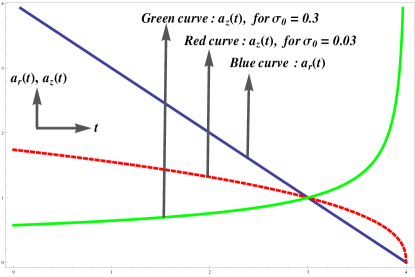
Figure 1: $a_{r}(t)$, $a_{z}(t)$ versus $t$

Figure (1) clearly demonstrates that $a_{r}(t)$ decreases with time linearly and goes to zero as $t$ tends to $t_{0}$. On the other hand $a_{z}(t)$ decreases almost uniformly until $t$ approaches a value close to $t_{0}$, where it hurries towards a zero proper volume singularity. This collapsing behaviour of $a_{z}(t)$ is shown in the dashed curve where $\sigma_{0}$ is taken as $0.03$. On the other hand, the green solid curve depicts the diverging character of $a_{z}(t)$ for $\sigma_{0}=0.3$.

4 Visibility of the singularity

The visibility of curvature singularity to an exterior observer depends on the formation of an apparent horizon. The condition for such a surface is given by

$$g^{\mu\nu}Z_{,\mu}Z_{,\nu}\bigg{|}_{r_{ah},t_{ah}}=0$$ (31)

where $Z$ is the proper radius of the two cylinder, given by $ra_{r}(t)$ in the present case, $r_{ah}$ and $t_{ah}$ being the comoving radial coordinate and time of formation of the apparent horizon respectively. Using the form of $g^{\mu\nu}$ presented in eqn.(7), above expression can be simplified and turns out to be,

$$r_{ah}^{2}\dot{a}_{r}(t_{ah})^{2}=1$$ (32)

where we use $a_{r}(t)=e^{[\alpha(t)+\sigma(t)]}$. Due to the solution of $a_{r}(t)$, eqn.(32) takes the following form :

$$\big{[}t_{0}-t_{ah}\big{]}=\frac{1}{4}B^{(r)}_{0}r_{ah}^{2}~{}~{}~{}~{}~{}~{}~{}~{}.$$ (33)

The above expression clearly demonstrates that $t_{ah}$ is less than $t_{0}$ (i.e. $t_{ah}<t_{0}$). Therefore the formation of apparent horizon lags behind than the formation of singularity. Thus, the curvature singularity discussed here is always covered from an exterior observer by the apparent horizon. At this stage, it may be mentioned that the singularity formed is not a central singularity, it is formed at any value of $r$ within the distribution. Such a singularity in general relativity is always covered by a horizon [54].

5 Matching of the interior spacetime with an exterior geometry

To complete the model, the interior spacetime geometry of the collapsing scalar field cylindrical cloud (recall that the interior geometry is cylindrically symmetric) needs to be matched to an exterior geometry. For the required matching, the Israel conditions are used, where the metric coefficients and extrinsic curvatures (first and second fundamental forms respectively) are matched at the boundary of the cylinder [55]. At this stage, it deserves mention that the Gauss-Bonnet term (controlled by the coupling function $\xi(\Phi)$) generates an effective energy momentum tensor which can not be zero (since it arises effectively from spacetime curvature) at the exterior and hence the presence of Gauss-Bonnet gravity spoils the matching of the collapsing interior spacetime with a vacuum exterior geometry. Such spoiling of matching (with a vacuum exterior) due to the presence of Gauss-Bonnet gravity can also be found in the previous literature [49]. In addition, the energy momentum tensor carried by the electromagnetic field will further lead to an inconsistency if the interior collapsing cloud is matched with a vacuum exterior. For instance, since vacuum has zero electromagnetic (em) field, such a matching would lead to a discontinuity in the em field, which means a delta function in the gradient of the em field. As a consequence, there will appear square of a delta function in the stress-energy, which is definitely an inconsistency. Keeping these in mind, here we match the interior geometry with a generalized cylindrically symmetric exterior spacetime [55, 56, 57] at the boundary hypersurface $\Sigma$ given by $r=r_{0}$. The metric inside and outside of $\Sigma$ are given by,

$$ds_{-}^{2}=-dt^{2}+e^{[2\alpha(t)+2\sigma(t)]}\bigg{(}dr^{2}+r^{2}d\theta^{2}\bigg{)}+e^{[2\alpha(t)-4\sigma(t)]}dz^{2}$$ (34)

and

$$ds_{+}^{2}=e^{2(\Upsilon-\Psi)}\big{(}-dT^{2}+d\rho^{2}\big{)}+R^{2}e^{-2\Psi}d\theta^{2}+e^{2\Psi}\big{(}dz+Wd\theta\big{)}^{2}$$ (35)

respectively, where $T,\rho,\theta$ and $z$ are the exterior coordinates and $\Upsilon$, $\Psi$, $R$, $W$ are functions of $T$ and $\rho$. Therefore $\frac{\partial}{\partial\theta}$ and $\frac{\partial}{\partial z}$ are the killing vector fields of the exterior spacetime which yields a cylindrical symmetry in the exterior. The same hypersurface $\Sigma$ can alternatively be defined by the exterior coordinates as $T=T(t)$ and $\rho=\rho(t)$. Then the metrics on $\Sigma$ from inside and outside coordinates turn out to be,

$$ds_{-,\Sigma}^{2}=-dt^{2}+e^{[2\alpha(t)+2\sigma(t)]}r_{0}^{2}d\theta^{2}+e^{[2\alpha(t)-4\sigma(t)]}dz^{2}$$

and

$$ds_{+,\Sigma}^{2}=e^{2(\Upsilon_{\Sigma}-\Psi_{\Sigma})}\big{(}-\dot{T}^{2}+\dot{\rho}^{2}\big{)}dt^{2}+R_{\Sigma}^{2}e^{-2\Psi_{\Sigma}}d\theta^{2}+e^{2\Psi_{\Sigma}}\big{(}dz+W_{\Sigma}d\theta\big{)}^{2}$$

where $\Upsilon_{\Sigma}(t)$ $\big{(}=\Upsilon(T(t),\rho(t))\big{)}$, $\Psi_{\Sigma}(t)$, $R_{\Sigma}(t)$ and $W_{\Sigma}(t)$ are the respective functions defined on $\Sigma$ and dot represents $\frac{d}{dt}$. Matching the first fundamental form on $\Sigma$ (i.e. $ds_{-,\Sigma}^{2}=ds_{+,\Sigma}^{2}$) yields the following conditions :

$$e^{2(\Upsilon_{\Sigma}-\Psi_{\Sigma})}\big{(}\dot{T}^{2}-\dot{\rho}^{2}\big{)}=1~{}~{}~{},$$ (36)

$$e^{\Psi_{\Sigma}(t)} = a_{z}(t)$$ (37)

$$= B^{(z)}_{0}(t_{0}-t)^{\frac{1}{2}-3\sigma_{0}}~{}~{}~{},$$

$$R_{\Sigma}(t) = r_{0}a_{r}(t)a_{z}(t)$$ (38)

$$= r_{0}B^{(r)}_{0}B^{(z)}_{0}(t_{0}-t)^{\frac{3}{2}-3\sigma_{0}}$$

and

$$W_{\Sigma}(t)=0.$$ (39)

In order to match the second fundamental form, we calculate the normal of the hypersurface $\Sigma$ from inside ($\vec{n}^{-}=n^{-}_{t}$, $n^{-}_{r}$, $n^{-}_{\theta}$, $n^{-}_{z}$) and outside ($\vec{n}^{+}=n^{+}_{T}$, $n^{+}_{\rho}$, $n^{+}_{\theta}$, $n^{+}_{z}$) coordinates as follows :

$$n^{-}_{t}=0~{}~{},~{}~{}~{}~{}~{}~{}~{}~{}n^{-}_{r}=a(t)~{}~{},~{}~{}~{}~{}~{}~{}~{}n^{-}_{\theta}=n^{-}_{z}=0$$ (40)

and

$$n^{+}_{T}=\frac{e^{(\Upsilon_{\Sigma}-\Psi_{\Sigma})}\dot{\rho}}{\sqrt{\dot{T}^{2}-\dot{\rho}^{2}}}~{}~{},$$

$$n^{+}_{\rho}=\frac{e^{(\Upsilon_{\Sigma}-\Psi_{\Sigma})}\dot{T}}{\sqrt{\dot{T}^{2}-\dot{\rho}^{2}}}~{}~{},$$

$$n^{+}_{\theta}=n^{+}_{z}=0.$$ (41)

The above expressions of $\vec{n}^{-}$ and $\vec{n}^{+}$ leads to the extrinsic curvature of $\Sigma$ from interior and exterior coordinates respectively, and are given by,

$$K_{tt}^{-}=0~{}~{},~{}~{}~{}~{}~{}~{}~{}~{}~{}K_{\theta\theta}^{-}=r_{0}a_{r}(t)~{}~{},~{}~{}~{}~{}~{}~{}~{}K_{zz}^{-}=0$$ (42)

(all the other components of $K_{\mu\nu}^{-}$ are zero) from interior metric, and

$$K_{tt}^{+}=e^{(\Upsilon_{\Sigma}-\Psi_{\Sigma})}\sqrt{\dot{T}^{2}-\dot{\rho}^{2}}\bigg{[}\big{(}\Psi_{\rho}\dot{T}-\Psi_{T}\dot{\rho}\big{)}-\big{(}\Upsilon_{\rho}\dot{T}-\Upsilon_{T}\dot{\rho}\big{)}\bigg{]}~{}~{},$$

$$K_{\theta\theta}^{+}=\frac{R_{\Sigma}e^{-(\Upsilon_{\Sigma}+\Psi_{\Sigma})}}{\sqrt{\dot{T}^{2}-\dot{\rho}^{2}}}\bigg{[}\big{(}R_{\rho}\dot{T}-R_{T}\dot{\rho}\big{)}-R_{\Sigma}\big{(}\Psi_{\rho}\dot{T}-\Psi_{T}\dot{\rho}\big{)}\bigg{]}~{}~{}~{}~{},$$

$$K_{zz}^{+}=\frac{e^{-(\Upsilon_{\Sigma}-3\Psi_{\Sigma})}}{\sqrt{\dot{T}^{2}-\dot{\rho}^{2}}}\bigg{[}\Psi_{\rho}\dot{T}-\Psi_{T}\dot{\rho}\bigg{]}~{}~{}~{}~{},$$

$$K_{z\theta}^{+} = K_{\theta z}^{+}$$ (43)

$$= \frac{e^{-(\Upsilon_{\Sigma}-3\Psi_{\Sigma})}}{\sqrt{\dot{T}^{2}-\dot{\rho}^{2}}}\bigg{[}W_{\rho}\dot{T}-W_{T}\dot{\rho}\bigg{]}$$

(all the other components of $K_{\mu\nu}^{+}$ are zero) from exterior metric, where the subscription denotes the respective derivative on the hypersurface $\Sigma$, such as $R_{T}=\frac{\partial R}{\partial T}\bigg{|}_{\Sigma}$.

The equality of the extrinsic curvatures at $\Sigma$ from both sides is therefore equivalent to the following conditions :

$$\bigg{[}R_{\rho}\dot{T}-R_{T}\dot{\rho}\big{)}\bigg{]}\frac{R_{\Sigma}e^{-(\Upsilon_{\Sigma}+\Psi_{\Sigma})}}{\sqrt{\dot{T}^{2}-\dot{\rho}^{2}}} = r_{0}a_{r}(t)$$ (44)

$$= r_{0}B^{(r)}_{0}(t_{0}-t)~{}~{}~{}~{}~{},$$

$$\bigg{[}\Upsilon_{\rho}\dot{T}-\Upsilon_{T}\dot{\rho}\bigg{]}=0~{}~{}~{}~{},$$ (45)

$$\bigg{[}\Psi_{\rho}\dot{T}-\Psi_{T}\dot{\rho}\bigg{]}=0~{}~{}~{}~{},$$ (46)

and

$$\bigg{[}W_{\rho}\dot{T}-W_{T}\dot{\rho}\bigg{]}=0.$$ (47)

Eqn.(44) can be further simplified by using the conditions obtained in eqn.(36), eqn.(37), eqn.(38) and finally we obtain the following expression

$$\bigg{[}R_{\rho}\dot{T}-R_{T}\dot{\rho}\bigg{]} = \frac{e^{2\Upsilon_{\Sigma}}}{a_{z}(t)}$$ (48)

$$= \frac{e^{2\Upsilon_{\Sigma}}}{B^{(z)}_{0}(t_{0}-t)^{\frac{1}{2}-3\sigma_{0}}}$$

The above four relations along with eqn.(36) to eqn.(39) completely specify the matching at the boundary of the collapsing scalar field with an exterior cylindrically symmetric geometry.

6 Conclusion

We consider a “Scalar-Maxwell-Einstein-Gauss-Bonnet” theory in four dimensions where the scalar field couples non-minimally with the Gauss-Bonnet (GB) term. This coupling with the scalar field guarantees the non topological character of the GB term. In this higher curvature theory, we examine the possible effects of the electromagnetic field on scalar field collapse.

The presence of electromagnetic field requires an anisotropic metric. We consider a special Bianchi-I metric $\big{(}$which possesses a cylindrical symmetry, the radial scale factor ($a_{r}(t)$) is different form the longitudinal scale factor ($a_{z}(t)$)$\big{)}$ as a candidate of an anisotropic model. With the aforementioned metric, an exact solution is obtained for the spacetime geometry, which clearly reveals that the radius of a two cylinder decreases monotonically with time. Therefore, the volume of the cylinder of the scalar field collapses and goes to zero at a finite time ($t_{0}$) leading to a zero proper volume singularity. From the behaviour of Kretschmann scalar, it is found that the singularity formed as a result of the collapse is a finite time curvature singularity.

On the other hand, the evolution of the longitudinal scale factor indicates that for $\sigma_{0}<1/6$, $a_{z}(t)$ decreases with time and goes to zero at $t\rightarrow t_{0}$ while the condition $\sigma_{0}>1/6$ makes $a_{z}(t)$ an increasing function of time and as a consequence, diverges at $t\rightarrow t_{0}$. The parameter $\sigma_{0}$ is essentially determined by the Gauss-Bonnet coupling (with the scalar field) $\xi_{0}$ and the parameters $V_{0}$, $\Phi_{0}$. However such collapsing or diverging behaviours of $a_{z}(t)$ demonstrate that the singularity we discussed here is point like or line like depending on the condition whether $\sigma_{0}<1/6$ or $\sigma_{0}>1/6$ respectively. Moreover, it may be mentioned that the parameter $\sigma_{0}$ actually regulates the strength of the spacetime anisotropy. Therefore it can be argued that in the present context, the pattern of the singularity (point like or line like) is controlled by the strength of anisotropy of the spacetime with the limiting situation is defined by $\sigma_{0}=1/6$. For such limiting case, $a_{z}(t)$ becomes constant (finite) which in turn leads the collapse to a “finite line singularity”. Further this limiting condition corresponds to $C=0$ (see eqn.(25)). Therefore the final state of the scalar field collapse in absence of the electromagnetic field is demonstrated by such “finite line singularity”.

The visibility of curvature singularity to an exterior observer depends on apparent horizon. The formation of apparent horizon is investigated and it turns out that the apparent horizon forms before the collapsing cloud hits to singularity. Therefore the curvature singularity is hidden from exterior by an apparent horizon. Here, it deserves mentioning that the singularity is independent of the radial coordinate $r$ and it is covered by a horizon. This result is consistent with the result obtained by Joshi et al [54] that unless one has a central singularity, it can not be a naked singularity. It is interesting to note that the result obtained in the present work in the presence of Gauss-Bonnet term is completely consistent with the corresponding GR result. Such consistency between Gauss-Bonnet gravity and Einstein’s GR is also in agreement with [49].

Finally, we match the interior collapsing spacetime geometry with a generalized cylindrically symmetric exterior geometry at the boundary of the cloud ($\Sigma$). For this matching, the Israel junction conditions are used where the metric coefficients and extrinsic curvatures are matched on $\Sigma$.

Appendix - I: Situation of isotropic spacetime

The non static isotropic metric ansatz is taken as,

$$ds^{2}=-dt^{2}+a^{2}(t)\bigg{[}dr^{2}+r^{2}d\theta^{2}+dz^{2}\bigg{]}$$ (49)

with $a(t)$ is the scale factor of the spacetime characterized by the coordinates $t$ ($=x^{0}$), $r$ ($=x^{1}$), $\theta$ ($=x^{2}$) and $z$ ($=x^{3}$) where $t$ is the timelike one. Moreover the scalar field and the electromagnetic field are considered to be dependent only on $t$. Therefore $F_{\mu\nu}$ has three non zero independent components : $F_{01}$, $F_{02}$ and $F_{03}$. With these non zero components of $F_{\mu\nu}$, we obtain various components of $T_{\mu\nu}(A)$ from eqn.(3) and are given by,

$$T_{00} = \frac{1}{2}\bigg{[}F_{01}F^{01}+F_{02}F^{02}+F_{03}F^{03}\bigg{]}$$

$$T_{11} = -\frac{1}{2}a^{2}\bigg{[}F_{01}F^{01}-F_{02}F^{02}-F_{03}F^{03}\bigg{]}$$

$$T_{22} = -\frac{1}{2}a^{2}\bigg{[}-F_{01}F^{01}+F_{02}F^{02}-F_{03}F^{03}\bigg{]}$$

$$T_{33} = -\frac{1}{2}a^{2}\bigg{[}-F_{01}F^{01}-F_{02}F^{02}+F_{03}F^{03}\bigg{]}$$

$$T_{10} = T_{20}=T_{30}=0$$

$$T_{12} = -a^{2}F_{01}F^{02}~{}~{}~{}~{}~{},~{}~{}~{}~{}T_{13}=-a^{2}F_{01}F^{03}~{}~{}~{}~{},~{}~{}~{}T_{23}=-a^{2}F_{02}F^{03}$$ (50)

Using the above expressions of $T_{\mu\nu}(A)$, the non diagonal components of gravitational equation are simplified to the following form :

$$F_{01}F^{02}=F_{01}F^{03}=F_{02}F^{03}=0$$ (51)

which has the solution as $F_{01}=F_{02}=F_{03}=0$. Thus a spatially flat isotropic spacetime cannot support the time dependent electromagnetic field. However a Bianchi-I spacetime, although it is spatially flat, can sustain the gauge field by virtue of its anisotropy.

References

- [1] J.R. Oppenheimer, H. Snyder, Phys. Rev. 56, 455 (1939).
- [2] B. Datt, Z. Phys. 108, 314 (1938). Reprinted as a Golden Oldie, Gen. Relativ. Gravit., 31, 1615 (1999)
- [3] P.S. Joshi, Global Aspects in Gravitation and Cosmology (Clarendon Press, Oxford, 1993).
- [4] P.S. Joshi. arXiv:1305.1005.
- [5] D. Christodoulou, Commun. Math. Phys. 109, 591, 613 (1987).
- [6] D. Christodoulou, Ann. Math. 140, 607 (1994).
- [7] S. Goncalves, I. Moss, Class. Quant. Gravit. 14, 2607 (1997).
- [8] R. Giambo, Class. Quant. Gravit. 22, 2295 (2005).
- [9] S. Goncalves, Phys. Rev. D 62, 124006 (2000).
- [10] R. Goswami, P.S. Joshi, Mod. Phys. Lett. A 22, 65 (2007).
- [11] K. Ganguly, N. Banerjee, Pramana 80, 439 (2013).
- [12] R.G. Cai, L.W. Ji, R.Q. Yang; Commun.Theor.Phys. 65 no.3, 329-334 (2016).
- [13] R.G. Cai, L.W. Ji, R.Q. Yang; Commun.Theor.Phys. 68 no.1, 67 (2017).
- [14] R.G. Cai, R.Q. Yang. arXiv:1602.00112.
- [15] R.G. Cai, R.Q. Yang. arXiv:1512.07095.
- [16] C. Gundlach, Critical phenomena in gravitational collapse: living reviews. Living Rev. Rel. 2, 4 (1999).
- [17] R. Goswami, P.S. Joshi, Phys. Rev. D. 65, 027502 (2004).
- [18] S. Chakrabarti, Gen Relativ Gravit 49:24 (2017).
- [19] N.Banerjee, S. Chakrabarti; Phys. Rev. D, 95, 024015 (2017)
- [20] D. Goldwirth, T. Piran, Phys. Rev. D 36, 3575 (1987).
- [21] M.W. Choptuik, Phys. Rev. Lett. 70, 9 (1993).
- [22] P.R. Brady, Class. Quant. Gravit. 11, 1255 (1995).
- [23] C. Gundlach, Phys. Rev. Lett. 75, 3214 (1995).
- [24] J.D. Bekenstein, Phys. Rev. D 4 2185, (1971).
- [25] J. Oppenheimer and G. Volkoff, Phys. Rev. 55 374, (1939).
- [26] L. Rosales, W. Barreto, C. Peralta and B. Rodriguez-Mueller, Phys. Rev. D 82 084014, (2010).
- [27] Thorne, K.S. ; Phys. Rev. 138, B251 (1965).
- [28] Ardavan, H., Partovi, M.H. ; Phys. Rev. D 16, 1664 (1977).
- [29] Stein-Schabes, J.A. ; Phys. Rev. D 31, 1838 (1985).
- [30] Germani, C., Tsagas, C.G. ; Phys. Rev. D 73, 064010 (2006).
- [31] Herrera, L., Santos, N.O. ; Phys. Rep. 286, 53 (1997).
- [32] Di Prisco, A., Herrera, L., Denmat, G.Le., MacCallum, M.A.H., San- tos, N.O. ; Phys. Rev. D 76, 064017 (2007).
- [33] Sharif, M., Bhatti, M.Z. ; Gen. Relativ. Gravit. 44, 281 (2012a).
- [34] Sharif, M., Bhatti, M.Z. ; Mod. Phys. Lett. A 27, 1250141 (2012b).
- [35] Sharif, M., Yousaf, Z. ; Can. J. Phys. 90, 865 (2012).
- [36] N. Banerjee, T.Paul ; Eur.Phys.J. C77 no.10, 672 (2017).
- [37] S. Nojiri, S.D. Odintsov ; Phys.Rept. 505 59-144 (2011).
- [38] S. Nojiri, S.D. Odintsov, V.K. Oikonomou ; Phys.Rept. 692 1-104 (2017).
- [39] T. P. Sotiriou and V. Faraoni, Rev.Mod.Phys.82, 451 497 (2010).
- [40] A.De Felice and S. Tsujikawa, Living Rev.Rel. 13, 3 (2010).
- [41] A.Paliathanasis, Class. Quant. Grav. 33no. 7, 075012 (2016).
- [42] S.Nojiri, S. D. Odintsov, Phys.Lett.B 631 (2005).
- [43] S.Nojiri, S. D. Odintsov, O.G.Gorbunova, J.Phys.A39, 6627 (2006).
- [44] G.Cognola, E. Elizalde, S. Nojiri, S.D. Odintsov, S.Zerbini, Phys.Rev. D73, 084007 (2006).
- [45] H. Maeda ; Phys.Rev. D73 104004 (2006).
- [46] N. Deppe, C.D. Leonard, T. Taves, G. Kunstatter, R.B. Mann ; Phys.Rev. D86 104011 (2012).
- [47] C.Lanczos; Z. Phys. 73 147 (1932); C.Lanczos; Annals Math. 39 842 (1938).
- [48] D.Lovelock; J. Math. Phys. 12 498 (1971).
- [49] N. Banerjee, T.Paul ; Eur.Phys.J. C78 no.2, 130 (2018).
- [50] R. Goswami, A.M. Nzioki, S.D. Maharaj, S.G. Ghosh; Phys. Rev. D, 90, 084011 (2014).
- [51] S. Chakrabarti, N. Banerjee ; Eur. Phys. J. C. 77:166 (2017)
- [52] S. Chakrabarti, N. Banerjee ; Gen Relativ Gravit 48:57 (2016)
- [53] S. Nojiri, S.D. Odintsov, M. Sasaki, Phys. Rev. D 71 123509, (2005).
- [54] P.S. Joshi, R. Goswami, N. Dadhich, Phys. Rev. D 70, 087502 (2004).
- [55] B.C. Nolan, , L.V. Nolan ; Class. Quantum Grav., 21 (15): 3693, (2004).
- [56] A. S. Kompaneets, Zh. Eksp. Teor. Fiz. 34, 953 (Sov.Phys. JETP 7 659, (1958)) (1958).
- [57] P. Jordan, J. Ehlers, and W. Kundt, Abh. Akad. Wiss. Mainz. Math. Naturwiss. Kl 2 (1960).
- [58] S. Chakraborty, S. SenGupta ; Phys.Rev. D89 no.2, 026003 (2014).