Semiclassical calculation of spectral correlation functions of chaotic systems

Abstract

We present a semiclassical approach to $n$-point spectral correlation functions of quantum systems whose classical dynamics is chaotic, for arbitrary $n$. The basic ingredients are sets of periodic orbits that have nearly the same action and therefore provide constructive interference. We calculate explicitly the first correlation functions, to leading orders in their energy arguments, for both unitary and orthogonal symmetry classes. The results agree with corresponding predictions from random matrix theory, thereby giving solid support to the conjecture of universality.

I Introduction

According to the Bohigas-Giannoni-Schmit (BGS) conjecture, put forward 30 years ago bgs (see also bgs2 ; bgs3 ), highly excited energy levels of generic chaotic systems have universal local spectral statistics. This universality is captured by the random matrix theory (RMT) approach to quantum chaos: such statistics are expected to agree with those of the Gaussian Ensembles, the particular ensemble (unitary, orthogonal or symplectic) being determined by the overall symmetries of the system haake . For spinless particles, the unitary class corresponds to systems with broken time-reversal symmetry (TRS), while the orthogonal class corresponds to systems with preserved TRS.

Obtaining spectral statistics for a specific system should be possible within the semiclassical approximation, by using the periodic orbit theory of the Gutzwiller trace formula gutz and ergodic properties of long orbits. Indeed, progress in this direction was made early on in hoda ; berry , deriving the leading term in $(\epsilon_{1}-\epsilon_{2})^{-1}$ of the $2$-point spectral correlation function $\mathcal{R}_{2}(\epsilon_{1}-\epsilon_{2})$ by considering only interference of an orbit with itself (so-called ‘diagonal approximation’). For time-reversal invariant systems also interference between mutually time-reversed orbits was taken into account.

Interference between orbits which are not identical up to time reversal was expected to give higher-order contributions, as conjectured and supported numerically in argaman . This interference started to be accounted for perturbatively in the work of Sieber and Richter sieber ; sieber2 , providing the next-to-leading term of $\mathcal{R}_{2}$. It was suggested that the mechanism producing systematic interference is the existence of ‘encounters’ in long orbits, regions of phase space where the orbit comes very close to itself, up to time reversal. This theory allowed the calculation of $\mathcal{R}_{2}$ for all universality classes, at all orders of perturbation theory R2a ; R2b ; R2c and even beyond perturbation theory longa ; km ; longb .

However, it is the semiclassical derivation of all $n$-point correlation functions, denoted $\mathcal{R}_{n}$, which would embody the full BGS conjecture. This has so far remained a challenge because it involves multiplets of correlated periodic orbits with $n$ different energies. An exception is taro where a variant of the diagonal approximation also accounting for non-perturbative effects was evaluated for the unitary symmetry class, however leaving out perturbative contributions due to encounters. (See also shukla for the standard diagonal approximation.) Interestingly, the analogous problem has evolved more rapidly in the transport setting combinat1 ; combinat2 ; combinat3 ; combinat4 ; combinat6 ; combinat7 ; combinat5 ; combinat8 , where the semiclassical calculation of counting statistics requires multiplets of correlated scattering trajectories, but all at the same energy (but energy correlations in scattering have also been considered energy1 ; energy2 ). We also note that for quantum graphs an understanding of higher-order correlation functions has been achieved in weidenmueller1 ; weidenmueller2 .

In this work we present substantial progress in the semiclassical calculation of $\mathcal{R}_{n}$, both for systems with and without TRS. First, we derive a set of diagrammatic rules that reduces the problem to the counting of certain diagrams which in turn, following previous works R2c ; combinat6 , we relate to factorizations of permutations. This allows, in principle, any finite order in perturbation theory to be obtained for all symmetry classes. We then present the explicit calculation of the leading orders for the first correlation functions, and show that the results agree with corresponding predictions from random matrix theory.

II Spectral correlation functions

II.1 Definition

Let $\rho(E)$ denote the system’s density of states. This can be divided into the smooth Weyl part $\bar{\rho}$, related to the volume of the energy shell in phase space, and a fluctuating part, $\rho(E)=\bar{\rho}(E)+\rho_{\rm fl}(E).$ Then

$$\mathcal{R}_{n}(\epsilon)=\frac{1}{\bar{\rho}^{n}}\left\langle\prod_{i=1}^{n}\rho\left(E+\frac{\epsilon_{i}}{\bar{\rho}}\right)\right\rangle$$ (1)

is the $n$-point correlation function expressed in terms of dimensionless energy differences $\epsilon_{i}$. The brackets denote an average with respect to $E$, over an interval small enough to neglect variations of $\bar{\rho}$.

It is easy to relate $\mathcal{R}_{n}(\epsilon)$ to a similar quantity, defined in terms of only the fluctuating part of the spectral density,

$$\widetilde{\mathcal{R}}_{n}(\epsilon)=\frac{1}{\bar{\rho}^{n}}\left\langle\prod_{i=1}^{n}\rho_{\rm fl}\left(E+\frac{\epsilon_{i}}{\bar{\rho}}\right)\right\rangle.$$ (2)

Since by definition $\rho_{\rm fl}$ has a vanishing average, we obtain $\widetilde{\mathcal{R}}_{1}=0$. Thus, we have, for example,

$$\mathcal{R}_{2}(\epsilon_{1},\epsilon_{2})=1+\widetilde{\mathcal{R}}_{2}(\epsilon_{1},\epsilon_{2})$$ (3)

and

$$\mathcal{R}_{3}(\epsilon_{1},\epsilon_{2},\epsilon_{3})=1+\sum_{j=1}^{3}\sum_{k>j}^{3}\widetilde{\mathcal{R}}_{2}(\epsilon_{j},\epsilon_{k})+\widetilde{\mathcal{R}}_{3}(\epsilon_{1},\epsilon_{2},\epsilon_{3}).$$ (4)

II.2 Results from random matrix theory

Correlation functions for the Gaussian ensembles have long been studied within random matrix theory, using different methods (see, e.g. Mehta ; Forrester ; brezin ; kanzieper ). In the regime of large matrices, the calculation of $\mathcal{R}_{n}$ for the Gaussian Unitary Ensemble reduces to the calculation of $n\times n$ determinants,

$$\mathcal{R}_{n}(\epsilon)=\det\left(\frac{\sin[\pi(\epsilon_{i}-\epsilon_{j})]}{\pi(\epsilon_{i}-\epsilon_{j})}\right).$$ (5)

For example,

$$\mathcal{R}_{2}(\epsilon_{1},\epsilon_{2}) =1-\left(\frac{\sin[\pi(\epsilon_{1}-\epsilon_{2})]}{\pi(\epsilon_{1}-\epsilon_{2})}\right)^{2}$$ (6)

$$=1+\frac{2}{\pi^{2}(\epsilon_{1}-\epsilon_{2})^{2}}-\frac{2\cos[2\pi(\epsilon_{1}-\epsilon_{2})]}{\pi^{2}(\epsilon_{1}-\epsilon_{2})^{2}}.$$ (7)

In general, $\mathcal{R}_{n}(\epsilon)$ can be divided into oscillatory and non-oscillatory terms, the former containing trigonometric functions of the variables $\epsilon_{i}-\epsilon_{j}$, and the latter being a Laurent polynomial in these variables.

The semiclassical approach we employ here, based on the Gutzwiller trace formula, is only able to address the non-oscillatory terms. More refined approaches, based on the so-called Riemann-Siegel look-alike formula, have been employed in order to derive the oscillatory terms. We believe the approach presented here may be adapted to this more general setting.

Systems with time-reversal symmetry are modeled by the Gaussian Orthogonal Ensemble. In that case the correlation functions are expressible as $2n\times 2n$ Pfaffians,

$$\mathcal{R}_{n}(\epsilon)={\rm Pf}\left(\begin{matrix}D(\epsilon_{i}-\epsilon_{j})&S(\epsilon_{i}-\epsilon_{j})\\ -S(\epsilon_{i}-\epsilon_{j})&I(\epsilon_{i}-\epsilon_{j})\end{matrix}\right),$$ (8)

Here the matrix consists of $2\times 2$ blocks labelled by $i,j=1\ldots n$, and the entries involve the functions

$$S(x)=\frac{\sin(\pi x)}{\pi x}$$ (9)

and

$$D(x)=\int_{0}^{1}du\,u\sin(\pi ux),\quad I(x)=-\int_{1}^{\infty}\frac{du}{u}\sin(\pi ux).$$ (10)

These correlations can also be divided into oscillatory and non-oscillatory terms, but the latter are now infinite series in the variables $(\epsilon_{i}-\epsilon_{j})^{-1}$. For example, the non-oscillatory terms for $\mathcal{R}_{2}$ in this class are

$$\mathcal{R}_{2}^{\rm no}(\epsilon_{1},\epsilon_{2})=1-\frac{1}{\pi^{2}(\epsilon_{1}-\epsilon_{2})^{2}}+\frac{3}{2{\pi}^{4}(\epsilon_{1}-\epsilon_{2})^{4}}+\cdots$$ (11)

Explicit formulas for $n>2$ will be given later, see Eqs. (49) and (53).

II.3 Semiclassical Approximation

A semiclassical approach to the problem is justified since we consider high-lying states. This must start from the celebrated Gutzwiller trace formula haake ; gutz , which asymptotically as $\hbar\to 0$ relates $\rho_{\rm fl}$ to the isolated and unstable periodic orbits of the classical dynamics:

$$\rho_{\rm fl}(E)\approx\frac{1}{\pi\hbar}{\rm Re}\sum_{p}F_{p}T_{p}^{\rm prim}e^{iS_{p}(E)/\hbar},$$ (12)

where $S_{p}$ and $T_{p}^{\rm prim}$ are the action and primitive period of the orbit $p$, respectively, while $F_{p}$ is a stability factor. (Following the notaton of longb , this involves the monodromy matrix and includes the complex Maslov phase factor). The primitive period coincides with the period $T_{p}$, unless the orbit involves multiple repetitions of a shorter orbit, in which case the period of the shorter orbit has to be used. However, for any given range of periods the number of orbits involving repetitions of shorter ones is negligible compared to the overall number of orbits, hence we can replace $T_{p}^{\rm prim}$ by $T_{p}$ without affecting the final result of our theory. Making this replacement and introducing the Heisenberg time

$$T_{H}=2\pi\hbar\bar{\rho}$$ (13)

we thus write (12) as

$$\rho_{\rm fl}(E)\approx\frac{1}{T_{H}}\Big{(}\sum_{p}F_{p}T_{p}e^{iS_{p}(E)/\hbar}+{\rm c.c.}\Big{)}.$$ (14)

To compute correlation functions, the infinite sum (14) must be inserted into $\widetilde{\mathcal{R}}_{n}$, leading to multiple sums over periodic orbits. For example, $\widetilde{\mathcal{R}}_{2}(\epsilon_{1},\epsilon_{2})$ is approximated by

$$\frac{2}{T_{H}^{2}}{\rm Re}\left\langle\sum_{p,q}F_{p}F^{*}_{q}T_{p}T_{q}e^{i(S_{p}(E_{1})-S_{q}(E_{2}))/\hbar}\right\rangle,$$ (15)

where $E_{j}=E+\epsilon_{j}/\bar{\rho}$. Crucially, the contributions from most pairs of orbits will oscillate rapidly as the energy is varied and are washed out by the energy average. This can only be avoided if the action difference is small, giving the exponent a chance of being stationary with respect to small changes in $E$.

In general, inserting the trace formula (14) into $\widetilde{\mathcal{R}}_{n}(\epsilon)$, Eq. (2), we obtain a multiple sum over periodic orbits. For each orbit sum we have to take into account the possibility that the action appears with a positive sign (corresponding to the initial term in Eq.(14)), or with a negative sign (corresponding to the complex conjugated term). It is thus useful to split $\widetilde{\mathcal{R}}_{n}(\epsilon)$ into contributions $\widetilde{\mathcal{R}}_{J,K}(\epsilon)$ where $J$ actions contribute with a positive sign, and $K=n-J$ actions contribute with a negative sign. In terms of these auxiliary quantities, we have

$$\widetilde{\mathcal{R}}_{n}(\epsilon)=\sum_{J=0}^{n}\widetilde{\mathcal{R}}_{J,n-J}(\epsilon)$$ (16)

To obtain a concrete formula for $\widetilde{\mathcal{R}}_{J,K}(\epsilon)$ we first consider the case that the first $J$ actions, associated to the energy increments $\epsilon_{1},\ldots,\epsilon_{J}$ contribute with a positive sign. We denote the corresponding orbits by $p_{1},\ldots,p_{J}$ and assemble them into a set $P$. The remaining $K$ actions, associated to increments $\epsilon_{J+1},\ldots,\epsilon_{n}$ and orbits from $Q=\{q_{1},\ldots,q_{K}\}$, contribute with a negative sign. With the notation

$$\eta_{k}=\epsilon_{J+k}.$$ (17)

for the latter increments we obtain

$$R_{J,K}(\epsilon,\eta)=\frac{1}{T_{H}^{n}}\left\langle\sum_{P,Q}F_{P}F^{*}_{Q}T_{P}T_{Q}e^{i\Delta S/\hbar}\right\rangle,$$ (18)

with the action difference

$$\Delta S=\sum_{j=1}^{J}S_{p_{j}}(E+\epsilon_{j}/\bar{\rho})-\sum_{k=1}^{K}S_{q_{k}}(E+\eta_{k}/\bar{\rho}).$$ (19)

In order to write the multiple sums in compact form, we have also defined collective stability factors and period products as $F_{P}=\prod_{p\in P}F_{p}$ and $T_{P}=\prod_{p\in P}T_{p}$.

To obtain $\widetilde{\mathcal{R}}_{J,K}(\epsilon)$ we have to consider all ways of splitting the $n$ orbits into $J$ orbits for which the action is taken with a positive sign and $K$ orbits where it is taken with a negative sign. This can be done by summing over all permutations of the $n$ energy increments. This operation turns $\widetilde{\mathcal{R}}_{n}$ into a symmetric function of all energy increments; in the following it will be denoted by the operator ${\rm Sym}_{n}$. However summing over all permutations is actually too much as this also involves exchanges among the $J$ energy increments associated to positive signs in the exponent, and among the $K$ increments associated to negative signs. To compensate this we have to divide out the number $J!K!$ if such exchanges and write

$$\widetilde{\mathcal{R}}_{J,K}(\epsilon)=\frac{1}{J!K!}{\rm Sym}_{n}\Big{[}R_{J,K}(\epsilon,\eta)\Big{]},$$ (20)

Given $\widetilde{\mathcal{R}}_{J,K}(\epsilon)$ we can then access $\widetilde{\mathcal{R}}_{n}(\epsilon)$ using (16). Here, the extreme cases $J=0$ and $J=n$ are not allowed in practice, as in these cases all orbits contribute with the same sign to $\Delta S$. Hence the absolute value of the action difference can never be small and the associated contributions vanish after averaging over the energy. The simplest examples are thus

$$\widetilde{\mathcal{R}}_{2}(\epsilon_{1},\epsilon_{2})=\widetilde{\mathcal{R}}_{1,1}(\epsilon_{1},\epsilon_{2}),$$ (21)

and

$$\widetilde{\mathcal{R}}_{3}(\epsilon_{1},\epsilon_{2},\epsilon_{3}) =\widetilde{\mathcal{R}}_{1,2}(\epsilon_{1},\epsilon_{2},\epsilon_{3})+\widetilde{\mathcal{R}}_{2,1}(\epsilon_{1},\epsilon_{2},\epsilon_{3})$$

$$=2{\rm Re}\widetilde{\mathcal{R}}_{1,2}(\epsilon_{1},\epsilon_{2},\epsilon_{3}).$$ (22)

As already argued, averaging over the energy annihilates every summand apart from those with small action differences, i.e. almost identical cumulative actions of $P$ and $Q$. The simplest and important case of identical orbits will be discussed in the next subsection. The general mechanism behind non-trivial action correlations has been analyzed extensively in previous works sieber ; sieber2 ; R2a ; R2b ; R2c ; longa ; longb . This is that each $q$-orbit must follow closely (up to time reversal) a certain $p$-orbit for a period of time. However it can switch to be close to a different $p$-orbit (or a different part of the same $p$-orbit) in what is called an encounter. An $\ell$-encounter is a region where $\ell$ stretches of $p$-orbits run nearly parallel (i.e. close in phase space) or anti-parallel (i.e. mutually time-reversed). The $q$-orbits then differ from the $p$-orbits by differently connecting the endpoints of these encounter stretches. (See Figures 1 and 2 for illustrations.) Outside the encounters the $q$-orbits are nearly equal to the $p$-orbits. In the following the orbit parts outside the encounters are referred to as links.

II.4 Diagonal Approximations

The simplest contribution to the average in (18) comes from the so-called diagonal approximation. For systems without TRS, this approximation accounts for the case that all orbits are pairwise equal, i.e. $P=Q$ (for $n=2$ this was considered in hoda ; berry ). This situation is only possible for $J=K$ and hence even $n$.

We start by considering two orbits $p$ and $q$ that are identical apart from having two slightly different energies $E_{p}=E+\epsilon/\bar{\rho}$ and $E_{q}=E+\eta/\bar{\rho}$. We can neglect differences between the periods $T_{p}$ and $T_{q},$ and between the stability factors $F_{p}$ and $F_{q}$. For the actions (whose difference will be divided by $\hbar\to 0$) we a have to be more careful and Taylor expand to linear order, using

$$\frac{\partial}{\partial\epsilon}S_{p}(E+\epsilon/\bar{\rho})=\frac{T_{p}}{\bar{\rho}}.$$ (23)

This leads to $S(E_{p})\approx S(E)+\epsilon T_{p}/\bar{\rho}$ and thus $\Delta S\approx(\epsilon-\eta)T_{p}/\bar{\rho}$. The contribution of two identical orbits to $R_{J,K}$ can now be evaluated using the Hannay-Ozorio de Almeida sum rule hoda . In the notation of longb this rule can be written as

$$\sum_{p}|F_{p}|^{2}f(T_{p})\approx\int_{0}^{\infty}\frac{dT}{T}f(T)$$ (24)

where $f$ represents any function of an orbit that depends only on its period.

The contribution of identical orbits can now be evaluated as

$$\frac{1}{T_{H}^{2}}\sum_{p}|F_{p}|^{2}T_{p}^{2}e^{i(\epsilon-\eta)T_{p}/\bar{\rho}\hbar} =\frac{1}{T_{H}^{2}}\int_{0}^{\infty}dTTe^{i(\epsilon-\eta)T/\bar{\rho}\hbar}$$

$$=-\frac{1}{4\pi^{2}(\epsilon-\eta)^{2}},$$ (25)

where the integral is regularized by adding a small positive imaginary part to $\epsilon$. For sets of orbits $P$ and $Q$ that coincide pairwise a factor of this type is obtained for each pair of orbits. For time-reversal invariant systems the result of (II.4) must be multiplied by 2 to account for pairs of mutually time-reversed orbits leading to

$$-\frac{1}{2\pi^{2}(\epsilon-\eta)^{2}}.$$ (26)

For $n>3$ there is also the possibility of partial diagonal approximations, in which only a few orbits coincide, i.e. we may have $P^{\prime}=Q^{\prime}$ with $P^{\prime}\subsetneq P$ and $Q^{\prime}\subsetneq Q$. The simplest such example is at $n=4$ and $J=K=2$ meaning that $P$ consists of two orbits $p_{1},p_{2}$ and $Q$ consists of two orbits $q_{1},q_{2}$. In this case $R_{2,2}(\epsilon,\eta)$ contains a contribution, denoted by $R_{2,2}^{(0)}$ from $P$, $Q$ in which no two orbits are the same. In addition there is a contribution from $P,Q$ that share one orbit,

$$-\frac{1}{4\pi^{2}}\Big{(} \frac{R^{(0)}_{1,1}(\epsilon_{2},\eta_{2})}{(\epsilon_{1}-\eta_{1})^{2}}+\frac{R_{1,1}^{(0)}(\epsilon_{2},\eta_{1})}{(\epsilon_{1}-\eta_{2})^{2}}$$

$$+ \frac{R^{(0)}_{1,1}(\epsilon_{1},\eta_{2})}{(\epsilon_{2}-\eta_{1})^{2}}+\frac{R_{1,1}^{(0)}(\epsilon_{1},\eta_{1})}{(\epsilon_{2}-\eta_{2})^{2}}\Big{)},$$ (27)

obtained by multiplying diagonal terms $-\frac{1}{4\pi^{2}(\epsilon_{j}-\eta_{k})^{2}}$ associated with two coinciding orbits with off-diagonal contributions $R_{1,1}^{(0)}$ accounting for the two remaining orbits. For each contribution, the off-diagonal factor must involve the energy increments not appearing in the diagonal factor. A final contribution arises from the case that all orbits coincide pairwise.

III Semiclassical diagrammatics

Using once more (23) we can rewrite (18) as

$$R_{J,K}(\epsilon,\eta)=\frac{(-1)^{K}}{(2\pi i)^{n}}\prod_{j=1}^{J}\frac{\partial}{\partial\epsilon_{j}}\prod_{k=1}^{K}\frac{\partial}{\partial\eta_{k}}\mathcal{A}_{J,K}(\epsilon,\eta),$$ (28)

where $\mathcal{A}_{J,K}(\epsilon,\eta)$ stands for the energy average

$$\mathcal{A}_{J,K}(\epsilon,\eta)=\left\langle\sum_{P,Q}F_{P}F_{Q}^{*}e^{i\Delta S/\hbar}\right\rangle.$$ (29)

In this Section we consider the situation when there are no coinciding orbits, i.e. we treat the quantity $R_{J,K}^{(0)}(\epsilon,\eta)$, and the analogously defined $\mathcal{A}^{(0)}_{J,K}(\epsilon,\eta)$.

The quantity $\Delta S$ has two contributions. The first one we have already met: the orbits have slightly different energies. This contribution can be approximated by

$$\sum_{j=1}^{J}T_{p_{j}}\epsilon_{j}/\bar{\rho}-\sum_{k=1}^{K}T_{q_{k}}\eta_{k}/\bar{\rho}.$$ (30)

The second contribution depends on the separation between the orbit stretches taking part in the encounters. For an encounter $e$ involving $\ell_{e}$ stretches, there are $\ell_{e}-1$ relative separations. For a system with two degrees of freedom, each of these can be decomposed into two components, pointing along the direction of the stable and unstable manifolds, denoted by $s_{e,m}$ and $u_{e,m}$. The second contribution to the action difference is then obtained as $\sum_{e}\sum_{m=1}^{\ell_{e}-1}s_{e,m}u_{e,m}$. For details of the derivation, and the definition of $s_{e,m}$ and $u_{e,m}$, we refer to R2c (based on TR ; Sp for $l_{e}=2$).

In the semiclassical limit the correlation functions are dominated by pairs of orbits with action differences at most of the order $\hbar$. As a consequence the separations in the relevant encounters are very small and the $p$ and $q$-orbits are very close inside the encounters as well as outside. As a consequence we can approximate $F_{Q}\approx F_{P}$ and hence $F_{P}F_{Q}^{*}\approx|F_{P}|^{2}$.

The sum over the set of correlated trajectories, $Q$, can now be replaced by an integral over an ergodic probability density, $w(s,u)$, determining the likelihood of encounters with given action difference. For the simplest correlation function, requiring only two orbits, this was done in detail in R2c (see the appendix of transport as well as handbook for the formulation using derivatives as in Eq. (28)) and yields (in our present notation)

$$\sum_{\rm struc}c_{\rm struc}\frac{(-1)^{V}}{(-2\pi i(\epsilon-\eta))^{L-V}},$$ (31)

as a semiclassical approximation to $\mathcal{A}_{1,1}^{(0)}(\epsilon,\eta)$. Here $V$ is the total number of encounters and $L$ is the total number of ‘links’, trajectory pieces connecting encounters.

The summation in (31) is over the possible topological structures that the encounters can produce. These structures are characterized by the number of encounters, the number of stretches belonging to each encounter, the way the encounter stretches are distributed among the orbits, and their ordering along the orbits. For time-reversal invariant systems they also depend on whether the encounter stretches point in the same direction or are time reversed. We will later see that the structures can be conveniently described in terms of permutations. The factor $c_{\rm struc}$ avoids overcounting due to some subtleties of the definition of structures that will be discussed at a later stage.

In the present situation of more general values of $J$ and $K$, an analogous calculation can be performed. Previous works longb have established that for orbits of periods $T_{p_{j}}$ a suitable probability density to find encounters associated to a given structure and with given stable and unstable separations is given by

$$w(s,u)=\frac{\prod_{j}T_{p_{j}}\int dt}{\prod_{e}\Omega^{\ell_{e}-1}t_{e}}.$$ (32)

Here $\Omega$ is the volume of the energy shell,

$$t_{e}=\frac{1}{\lambda}\ln\frac{c^{2}}{\min_{m}|s_{e,m}|\min_{n}|u_{e,n}|}$$ (33)

is the duration of the encounter $e$, $\lambda$ is the Lyapunov exponent of the system, and $c$ is a constant that will be irrelevant for the final result. $\int dt$ denotes a multiple integral over all times at which the orbits in $Q$ traverse the encounters, reckoned from a reference traversal. Now the sum over $Q$ for each given $P$ can be replaced by an integral over the density $w(s,u)$. Finally, the remaining sum over $P$ is evaluated using the Hannay-Ozorio de Almeida sum rule (24). The contribution to the sum $\left\langle\sum_{P,Q}F_{P}F_{Q}^{*}e^{i\Delta S/\hbar}\right\rangle$ from each structure is

$$\int_{0}^{\infty}\frac{dT_{p_{1}}}{T_{p_{1}}}...\int_{0}^{\infty}\frac{dT_{p_{J}}}{T_{p_{J}}}\int\prod_{e}\prod_{m=1}^{\ell_{e}-1}ds_{e,m}du_{e,m}w(s,u)\exp\left(\frac{i}{\hbar}\left[\sum_{j=1}^{J}\frac{T_{p_{j}}\epsilon_{j}}{\bar{\rho}}-\sum_{k=1}^{K}\frac{T_{q_{k}}\eta_{k}}{\bar{\rho}}+\sum_{e}\sum_{m=1}^{\ell_{e}-1}s_{e,m}u_{e,m}\right]\right).$$

Luckily, this expression factorizes nicely into contributions associated to encounters and links. The divisors $T_{p_{j}}$ cancel with the corresponding factors in $w(s,u)$. Afterwards the integrals over orbit periods and the integrals over encounter traversal times in $w(s,u)$ can be transformed into integrals over link durations, which we again denote by $t$. The only contribution of a link to the action difference is due to the different energy increments. A link that belongs to the orbit $p_{j}$ of $P$ and the orbit $q_{k}$ of $Q$ gives a contribution $t(\epsilon_{j}-\eta_{k})/\bar{\rho}$ to $\Delta S$. If we integrate and incorporate as a factor the inverse of the Heisenberg time, we obtain

$$T_{H}^{-1}\int dte^{it(\epsilon_{j}-\eta_{k})/(\hbar\bar{\rho})}=-\frac{1}{2\pi i(\epsilon_{j}-\eta_{k})}.$$ (34)

The contribution of each encounter to $\sum_{j=1}^{J}T_{p_{j}}\epsilon_{j}/\bar{\rho}-\sum_{k=1}^{K}T_{q_{k}}\eta_{k}/\bar{\rho}$ depends on the numbers of stretches it involves that form part of the different orbits. We assume that the encounter involves $\ell_{j}$ stretches of each of the orbits $p_{j}$, and after changing connections it involves $\widetilde{\ell}_{k}$ stretches of each of the orbits $q_{k}$ (with $\sum_{j}\ell_{j}=\sum_{k}\widetilde{\ell}_{k}=\ell)$. Then its contribution to the above sum can be written as $(\sum_{j}\ell_{j}\epsilon_{j}-\sum_{k}\widetilde{\ell}_{k}\eta_{k})t_{e}/\bar{\rho}$.

To obtain the contribution to $\mathcal{A}^{(0)}_{J,K}(\epsilon,\eta)$ must also take into account the remaining part of the action difference given by $\sum_{e}\sum_{m=1}^{\ell_{e}-1}s_{e,m}u_{e,m}$, the density $w(s,u)$ as well as factors $T_{H}^{\ell}$ that will altogether compensate the factor inserted in the link contribution. When all of this is taken into account we arrive at a factor

$$T_{H}^{\ell}\int d^{\ell-1}s\,d^{\ell-1}u\frac{1}{\Omega^{\ell-1}t_{{e}}}\exp\Big{[}{i\sum_{m}u_{m}s_{m}/\hbar}+\Big{(}\sum_{j}\ell_{j}\epsilon_{j}-\sum_{k}\widetilde{\ell}_{k}\eta_{k}\Big{)}t_{e}/(\bar{\rho}\hbar)\Big{]}\approx 2\pi i\Big{(}\sum_{j}\ell_{j}\epsilon_{j}-\sum_{k}\widetilde{\ell}_{k}\eta_{k}\Big{)}$$ (35)

arising from every encounter (where we suppressed the subscripts $e$ of $\ell$, $s$, and $u$).

As in previous works, the above integral is computed by expanding the $t_{e}$-dependent part of the exponential into a power series. Contributions relevant in the semiclassical limit arise only from the linear term in that expansion. They can be calculated by noting that the factor $t_{e}$ is canceled by the divisor $t_{e}$ in front of the exponential, and furthermore using $\int dudse^{ius/\hbar}=2\pi\hbar$ and $\bar{\rho}=\frac{\Omega}{(2\pi\hbar)^{2}}$. By contrast, the integral of the leading term in the expansion leads to a result that vanishes after averaging over the energy, and the higher-order terms are negligible in the semiclassical limit.

The factor (35) associated with an encounter can also be written in a slightly different but equivalent and technically advantageous way. To do so we single out one of the $\ell$ points where the orbit enters this encounter as the ‘first’. Say this point (and the preceding link) belongs to a certain $p_{j}$ and a certain $q_{k}$. If we assign to the encounter a factor

$$2\pi i(\epsilon_{j}-\eta_{k})$$ (36)

and sum over all choices of first stretches, we obtain the same result as (35), since in this sum each index $j$ arises $\ell_{j}$ times and each index $k$ arises $\widetilde{\ell}_{k}$ times. Hence, these two ways of dealing with the encounter factor are equivalent. However, this second method (assigning to the encounter a quantity which depends on its ‘first’ stretch and then summing over all possible first stretches) is more convenient, because the encounter factors become inverse to link factors and just compensate the links that are the first to arrive at the encounter.

In line with the above discussion, let $M_{jk}$ be the number of times orbits $p_{j}$ and $q_{k}$ run together in a link but are not the first ones to arrive at an encounter. Then each of these $M_{jk}$ links gives a factor $-\frac{1}{2\pi i(\epsilon_{j}-\eta_{k})}$, see (34). The encounter contributions (36) are cancelled apart from a factor $-1$ per encounter. Altogether, summation over structures thus gives the semiclassical approximation

$$\mathcal{A}_{J,K}^{(0)}(\epsilon,\eta) =\sum_{\rm struc}\prod_{jk}c_{\rm struc}\frac{(-1)^{V}}{(-2\pi i(\epsilon_{j}-\eta_{k}))^{M_{jk}}}$$ (37)

$$=\sum_{\rm struc}\frac{(-1)^{L}}{(2i\pi)^{L-V}}\prod_{jk}c_{\rm struc}\,z_{jk}^{M_{jk}}.$$ (38)

Here we have denoted the number of encounters by $V$, the number of links by $L$, and used that $\sum_{jk}M_{jk}=L-V$. We have also introduced

$$z_{jk}=\frac{1}{\epsilon_{j}-\eta_{k}}.$$ (39)

The quantity $c_{\rm struc}$ will be discussed properly in the next Sections; in particular, it depends on whether the system is time-reversal invariant or not.

Finally $R^{(0)}_{J,K}(\epsilon,\eta)$ can be accessed from these results by performing the derivatives given in (28). If we absorb these derivatives in

$$D_{J,K}=\frac{(-1)^{K}}{(2\pi i)^{n}}\prod_{j=1}^{J}\frac{\partial}{\partial\epsilon_{j}}\prod_{k=1}^{K}\frac{\partial}{\partial\eta_{k}},$$ (40)

we can write our semiclassical result for $R^{(0)}_{J,K}(\epsilon,\eta)$ as

$$D_{J,K}\Big{[}\mathcal{A}_{J,K}^{(0)}\Big{]}.$$ (41)

IV Structures and permutations, for broken TRS

In order to formalize the concept of a structure, it is useful to introduce permutations R2a ; R2b ; R2c ; combinat1 ; combinat2 ; combinat3 ; combinat4 . We number the encounter stretches in $P$, from $1$ to $L$, in such a way that inside the encounters the trajectories in $Q$ go from the beginning of stretch $i$ to the end of stretch $i+1$. The beginning of the final stretch of each encounter is then connected to the end of the initial one. This mapping can be expressed by a permutation $\sigma$. It is useful to reduce the freedom in ordering the encounters by requiring that longer ones come first. In this way, we associate with the set of encounters a permutation $\sigma$ whose cycles are

$$\sigma=(12\cdots\ell_{1})(\ell_{1}+1\cdots\ell_{1}+\ell_{2})\cdots,$$ (42)

where $\ell_{1}\geq\ell_{2}\geq\cdots$ are the encounter sizes.

On the other hand, we associate with $P$ the permutation $\pi$ which takes $i$ to $j$ if there is a link from the end of stretch $i$ to the beginning of stretch $j$. Successive application of $\pi$ hence yields the encounter stretches included in each of the orbits of $P$. Thus, clearly the cycles of $\pi$ correspond to the orbits in $P$.

Finally, we associate with trajectories $Q$ the permutation $\rho$ which is the product $\rho=\pi\sigma$. (Here products of permutations are defined such that when they are applied to a number the right-most factor is applied first.)

Applying this product to the index of the start point of an encounter stretch leads first to the end point it is connected to along $Q,$ and then to the start point of the stretch following the next link. Repeated application thus enumerates the start points in the order they are visited by $Q$. The cycles of $\rho$ are therefore in one-to-one relation to the orbits in $Q$.

Notice that there is still freedom in the relative order of encounters of the same size. Also, we must choose the first stretch in each encounter, which will be labelled by the smallest number. These different choices do not alter the permutation $\sigma$, but may alter $\pi$ and $\rho$. We will take into account all possible such choices. It is crucial to make sure that this does not lead to overcounting of the contributions to the correlation function. If we denote the number of encounters with $\ell$ stretches by $v_{\ell}$, there are $v_{\ell}!$ ways of ordering these encounters. To avoid overcounting, we thus have to divide out $v_{\ell}!.$ (Note that we could equivalently have left the ordering of encounters completely unspecified, and then divided by the factorial $V!$ of the overall number of encounters.) As already described earlier, we take into account all choices of a first stretch inside each encounter. However we have already modified the contribution of the encounter such that summation over all these choices leads to the correct encounter factor derived from semiclassics. Hence no further corrections are necessary and the factor $c_{\rm struc}$ in (41) has to be chosen as

$$c_{\rm struc}=\frac{1}{\prod_{\ell}v_{\ell}!}.$$ (43)

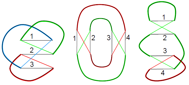
Figure 1: (color online) Correlated periodic orbits. Encounters are grossly exaggerated. Orbits in set $P$ are depicted in black lines, orbits in $Q$ in colored/grey lines. Left diagram has $J=1$, $K=3$; only one structure is possible. Middle diagram has $J=K=2$; two structures are possible, one of them is shown. Right diagram also has $J=K=2$; only one structure.

The example in Figure 1 can help visualize the permutations we have introduced. In the first diagram, the encounter permutation is $\sigma=(123)$, the permutation associated with the black orbit (the only member of $P$) is $\pi=(132)$, and the permutation associated with the three colored (grey) orbits (forming $Q$) is $\rho=\pi\sigma=(1)(2)(3)$. This diagram has only one possible choice of permutations, because changing the first stretch does not change either of the permutations.

In the second diagram, with the labels shown in the figure, we have $\sigma=(12)(34)$, $\pi=(14)(23)$ and $\rho=(13)(24)$. However, there is an equivalent choice of the permutations $\pi$ and $\sigma$: $\pi=(13)(24)$ and $\rho=(14)(23)$. Here the labels of the stretches 3 and 4 are exchanged. This leads to a different structure that has to be taken into account separately.

The last diagram also has $\sigma=(12)(34)$, but it admits four different choices of the remaining permutations: $\pi=(123)(4)$, $\rho=(134)(2)$; $\pi=(124)(3)$, $\rho=(143)(2)$; $\pi=(132)(4)$, $\rho=(1)(234)$; $\pi=(142)(3)$, $\rho=(1)(243)$.

The permutation $\sigma$ is fixed once the encounter sizes are known, and the equation $\sigma=\pi^{-1}\rho$ can be seen as a factorization of $\sigma$. As in the final two examples above, different choices of first stretch inside each encounter produce different structures if they lead to different factorizations. On the other hand, if we exchange e.g. $1\leftrightarrow 3$, $2\leftrightarrow 4$ in the middle diagram of Figure 1 this simply exchanges the encounters and does not lead to a different factorization or structure.

The calculation of $\mathcal{A}_{J,K}^{(0)}$ requires factorizations of specific permutations, of the kind seen in Eq.(42). In these factorizations, the first factor, $\pi^{-1}$, must have $J$ cycles, while the second factor, $\rho$, must have $K$ cycles, respectively corresponding to the orbits of $P$ and $Q$. The factorization must take place in the group of permutations of $L$ symbols (the number of links), and $\sigma$ must have $V$ cycles (the number of encounters). Notice that $\sigma$ cannot have fixed points, since encounters have size at least $2$. Therefore, for a given order in perturbation theory, i.e. for a fixed value of $L-V$, there exist only a finite number of factorizations.

Each structure is then characterized by (i) a choice of the permutations $\sigma$, $\pi$ and $\rho$ subject to these requirements, but crucially also (ii) one choice of assigning the $J$ ($K$) cycles of $\pi$ ($\rho$) to the $J$ ($K$) orbits in $P$ ($Q$).

V Structures and permutations, for preserved TRS

The structures arising for time-reversal invariant systems can also be described in terms of permutations. In this case we also have to account for the different directions of motion. The resulting permutations will describe the connections of the orbits in $P$ and $Q$ as well as their time-reversed versions.

To define the encounter permutations $\sigma$, we arbitrarily single out one preferred direction of motion inside each encounter. We then label the stretches in that direction of motion (belonging either to the orbits of $P$ or their time-reversed versions) by consecutive integers. The time-reversed version of each stretch, going opposite to the preferred direction, is indicated by the same integer but with an overbar. So the start of stretch $\overline{a}$ has the same position (but opposite sense of motion) as the end of stretch $a$, and the end of stretch $\overline{a}$ coincides with the beginning of stretch $a$ (again up to sense of motion).

The permutation $\sigma$ maps the start point of each stretch to the endpoint it is connected to within $Q$, i.e., after switching connections.

As before, the connections of the stretches in the preferred direction are indicated by cycles $(12\cdots\ell_{1})(\ell_{1}+1\cdots\ell_{1}+\ell_{2})\cdots$. If a stretch connects the start of $a$ to the end of $b$, its time-reversed will connect the start of the time-reversed of $b$, denoted by $\bar{b}$, to the end of $\bar{a}$. Hence each cycle is accompanied by one with all elements barred and reversed in order, leading to

$$\sigma=(12\cdots\ell_{1})(\ell_{1}+1\cdots\ell_{1}+\ell_{2})\cdots$$ (44)

$$\cdots(\overline{\ell_{1}+\ell_{2}}\cdots\overline{\ell_{1}+1})(\bar{\ell}_{1}\cdots\bar{2}\bar{1}).$$

The permutation $\pi$ determines how the end points of encounters are connected to start points through links. $\pi$ may map indices with bars to indices without or the other way around; this happens for example if the link returns to the same encounter but with opposite sense of motion, or if it leads to a different encounter but the preferred directions of motion in these encounters are not aligned. Similarly as above, if $\pi$ maps a given end point to a given start, $a\to b$, it induces the opposite mapping between the time-reversed versions of these points, $\bar{b}\to\bar{a}$. (Note that we define $\overline{\overline{a}}=a$.) Hence a cycle of the form, say, $(ab\bar{c})$ will be accompanied by a second cycle of the form $(c\bar{b}\bar{a})$. This is the only restriction on the form of $\pi$.

As inside each encounter of $P$ (or its time-reversed) every start point is connected to the end point with the same index, application of $\pi$ enumerates the start points in the order of traversal by $P$ and its time reversed. Hence every cycle of $\pi$ will correspond to a periodic orbit in $P$ or its time reversed. Pairs of cycles like $(ab\bar{c})$ and $(c\bar{b}\bar{a})$ describe mutually time-reversed orbits.

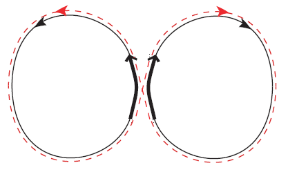
Figure 2: (color online) Diagram giving the leading contribution to $\mathcal{R}_{3}$ (encounters are grossly exaggerated). There is one orbit, depicted by a dashed line, correlated with two others, depicted by a full line. (Figure from longb .)

In analogy to systems without time-reversal invariance, the product $\rho=\pi\sigma$ maps the start point of each encounter stretch to the start point of the stretch following along $Q$ or its time-reversed. The cycles of $\rho$ come in pairs where one cycle describes an orbit in $Q$ and the other one describes its time-reversed version. (The relation between the cycles of $\rho$ is more complex than for $\sigma$ and $\pi$, and it does not lead to any further constraints on the factorizations used.)

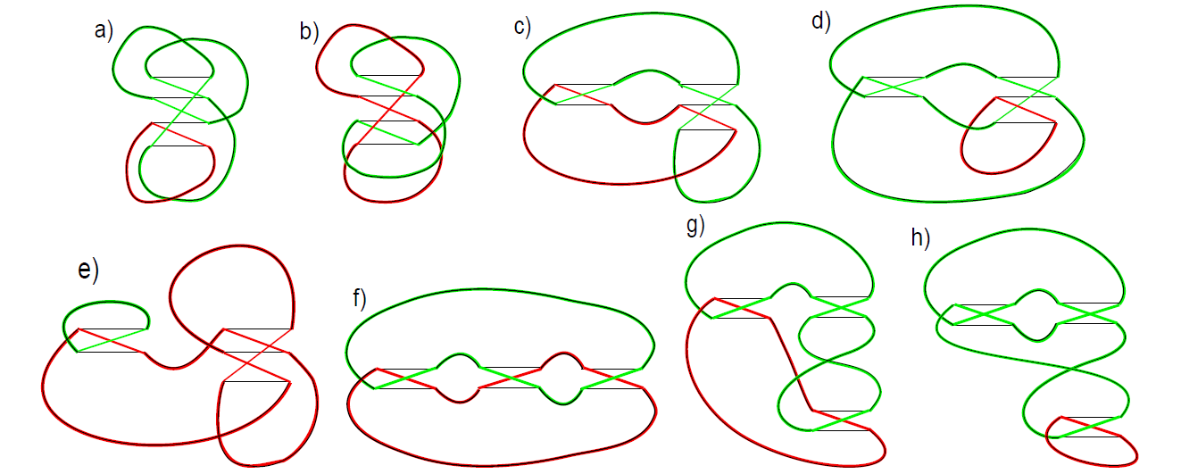
Figure 3: (color online) Diagrams depicting correlated periodic orbits contributing to the third order perturbation theory calculation of $\mathcal{R}_{3}$ (encounters are grossly exaggerated). In every case we have one orbit, in black, correlated with two others, in red and green (grey).

In the permutations thus defined, the orbits and their time-reversals are treated on equal footing. For each pair of time-reversed orbits described by $\pi$ there are two possible choices for the orbit to be included in $P$. Similarly for each pair of orbits described by $\rho$ there are two choices for the orbit to be included in $Q$. Hence, if we want to sum over all choices for $P$ and $Q$, we have to include a factor $2^{J+K}$, where $J$ is the number of orbits in $P$ (half the number of cycles in $\pi$) and $K$ is the number of orbits in $Q$ (half the number of cycles in $\rho$). On the other hand, for every choice of $P,Q$ we take into account all $2^{V}$ ways of fixing preferred directions inside the encounters. To avoid overcounting, we have to divide out $2^{V}$. Together with the division by $\prod_{\ell}v_{\ell}!$ explained earlier, we thus need a factor

$$c_{\rm struc}=\frac{2^{J+K-V}}{\prod_{\ell}v_{\ell}!}.$$ (45)

VI Leading orders, broken TRS

Our diagrammatic rule, Eq.(41), can be used for both unitary and orthogonal universality classes. By constructing the simplest diagrams explicitly (or finding the relevant factorizations), it is possible to obtain the first orders in perturbation theory.

For the unitary class, corresponding to broken time-reversal symmetry, the leading order approximation to $\mathcal{R}_{n}$, stemming from the diagonal approximation, has been obtained by Nagao and Müller taro . It turns out that this ‘approximation’ is in exact agreement with the prediction from random matrix theory. Here we show that the first few perturbative corrections indeed vanish for the simplest functions.

VI.1 $2$-point function

The $2$-point function has already been the subject of many papers, the closest one to the present approach being R2c . We discuss it again briefly.

The difference between the present approach and the one in R2c is in the concept of structure and in the way the encounter stretches are numbered. Since there is only one orbit in the set $P$, it made sense in R2c to just number the stretches in the order they were visited by that orbit (the same convention was also used in combinat3 ). As a result, this set was always represented by the permutation $P_{\rm loop}=(12\cdots L)$ and structures were identified with factorizations of this permutation in which one of the factors was also a single-cycle permutation, representing the single-orbit set $Q$.

In this work, we are fixing the encounter permutation to be of the form of Eq. (42). Therefore, neither of the single-cycle permutations representing $P$ or $Q$ need be given by $(12\cdots L)$. Instead, we define structures in terms of factorizations of $\sigma$ into single-cycle factors.

In R2c it was shown that all off-diagonal contributions to the 2-point function cancel for systems without TRS. We want to briefly discuss how this plays out in the leading off-diagonal order with our present conventions. As in R2a this order is determined by a diagram involving one 3-encounter and a diagram involving two 2-encounters. The former diagram has one structure described by the permutations $\rho=(123)$, $\pi=(123)$, $\rho=(132)$, and the latter diagram has two structures with $\sigma=(12)(34)$, $\pi=(1423)$, $\rho=(1324)$ and $\sigma=(12)(34)$, $\pi=(1324)$, $\rho=(1423)$. Their contributions to $\mathcal{A}^{(0)}_{11}$ cancel as the factor $\frac{(-1)^{L}}{\prod_{\ell}v_{\ell}!}$ from Eqs. (38) and (43) is equal to $-1$ for the first diagram and equal to $\frac{1}{2}$ for both structures of the second diagram.

VI.2 $3$-point function

The leading-order correction to the $3$-point correlation function $\mathcal{R}_{3}$ consists in a single diagram, where $P$ contains a single orbit with a single $2$-encounter, correlated with two orbits in the set $Q$, see Figure 2. This possibility has a single structure, associated with $\sigma=(12)$, $\pi=(12)$, $\rho=(1)(2)$, i.e. the factorization $(12)=(12)\cdot(1)(2)$. One of the orbits in $Q$ is always the first to arrive at the encounter, so the semiclassical contribution is proportional to either $z_{11}=(\epsilon_{1}-\eta_{1})^{-1}$ or $z_{12}=(\epsilon_{1}-\eta_{2})^{-1}$. In any case, it depends only on two variables. When we act with the operator $D_{12}\propto\partial^{3}/\partial\epsilon_{1}\partial\eta_{1}\partial\eta_{2}$, as required by (41), the final result vanishes. The same happens if the single orbit is taken as the only element of $Q$ and the two orbits are included in $P$.

This mechanism is quite general. According to (41), we must take derivatives with respect to all energies. But when a structure contains an orbit which participates in only one encounter, and it is the first one to arrive at that encounter, the quantity $\prod_{jk}z_{jk}^{M_{jk}}$ is independent of the energy of that orbit, and the derivative vanishes.

	$\sigma$	$\pi$	$\rho=\pi\sigma$	mult.
(a)	(1234)	(1243)	(142)(3)	3
	(1234)	(1342)	(1)(243)	1
(b)	(1234)	(1234)	(13)(24)	1
(c)	(123)(45)	(12534)	(15)(243)	5
	(123)(45)	(12435)	(14)(253)	1
(d)	(123)(45)	(13425)	(1524)(3)	4
	(123)(45)	(14352)	(1)(2534)	2
(e)	(123)(45)	(12345)	(1324)(5)	3
	(123)(45)	(12354)	(1325)(4)	3
(f)	(12)(34)(56)	(146235)	(136)(245)	6
	(12)(34)(56)	(145236)	(135)(246)	2
(g)	(12)(34)(56)	(162453)	(14)(2635)	18
	(12)(34)(56)	(162354)	(13)(2645)	6
(h)	(12)(34)(56)	(162345)	(13526)(4)	24
	(12)(34)(56)	(162435)	(14526)(3)	24

Table 1: Structures associated to the diagrams of Figure 3. Encounters are represented by a permutation $\sigma$, the black orbit by $\pi$ and the other orbits by $\rho$. The structures marked in grey give contributions that vanish after taking derivatives.

The above contribution involved $L-V=1$, and a simple argument involving the parities of permutations shows that for systems without TRS every second value of $L-V$ does not have any associated diagrams. (The parity of a permutation with $L$ elements and $C$ cycles is given by $(-1)^{L-C}$. Hence the parities of $\pi$, $\rho$ and $\sigma$ are given by $(-1)^{L-J}$, $(-1)^{L-K}$ and $(-1)^{L-V}$; using $\rho=\pi\sigma$ one can then show that $L-V$ must be even if $J-K$ is even and odd otherwise.) Hence the next correction to $\mathcal{R}_{3}$ arises from $L-V=3$. In Figure 3, we sketch the correlated sets of periodic orbits that are important in this case. There are two diagrams with a single $4$-encounter. One of them has four possible choices of permutations, while the other admits a single choice. There are three diagrams (altogether 18 choices of permutations) with a $2$-encounter and a $3$-encounter, and three other diagrams (altogether 80 choices) with three $2$-encounters.

In Table 1 we present all the permutations/structures that the diagrams in Figure 3 may have. The diagrams allow for different choices of permutations that can give different contributions. In the table we are displaying one representative choice for each contribution, and we give the number of overall choices with the same contribution in the final column. For example the additional choices of permutations for diagram (a) are $\pi=(1324)$, $\rho=(143)(2)$ and $\pi=(1423)$, $\rho=(132)(4)$. The contributions marked in grey are proportional to $z_{11}^{3}$ and hence vanish after taking derivatives. Notice how in all these structures the permutation $\rho$ has a cycle involving only numbers which begin a cycle in $\sigma$.

The contributions of the remaining structures in Table 1 to $\mathcal{A}^{(0)}_{1,2}$ are proportional to $z_{11}^{2}z_{12}$ or to $z_{11}z_{12}^{2}$, depending on how the energy increments $\eta_{1}$ and $\eta_{2}$ are assigned to the orbits. The result after symmetrization is proportional to ${\cal N}(z_{11}^{2}z_{12}+z_{11}z_{12}^{2})$. Here $\mathcal{N}$ is the sum over structures taking into account the multiplicities in the table as well as the weight $\frac{(-1)^{L}}{\prod_{\ell}v_{\ell}!}$ arising from (38) and (43), with $V$ the total number of permuted elements. The latter weight gives a minus sign for diagrams (c) and (e), and a factor $\frac{1}{6}$ for diagrams (f) to (h). It is easy to read off Table I that $\mathcal{N}$ is equal to $\mathcal{N}=3+1-5-4-3+1+3+4=0,$ as expected.

VI.3 4-point function

The leading order correction to the $4$-point correlation function has $L-V=2$. Let us consider separately the quantities $\mathcal{A}^{(0)}_{1,3}$ and $\mathcal{A}^{(0)}_{2,2}$.

The former has two different contributing diagrams. One diagram has a single $3$-encounter and only one possible structure; this is the first diagram shown in Figure 1. The other diagram has two $2$-encounters, hence $\sigma=(12)(34)$, and three choices of permutations: $\pi=(1234)$, $\rho=(13)(2)(4)$; $\pi=(1342)$, $\rho=(1)(23)(4)$; $\pi=(1432)$, $\rho=(1)(24)(3)$. All of these have vanishing contributions. These arise from derivatives of terms proportional to $z_{1k}z_{1k^{\prime}}$ (where $k,k^{\prime}=1,2,3$), which must vanish as at least one of the choices $1,2,3$ for the second index is absent.

	$\sigma$	$\pi$	$\rho=\pi\sigma$	mult.
(a)	(123)	(13)(2)	(12)(3)	1
	(123)	(12)(3)	(1)(23)	1
	(123)	(1)(23)	(13)(2)	1
(b)	(12)(34)	(134)(2)	(123)(4)	2
	(12)(34)	(143)(2)	(124)(3)	2
	(12)(34)	(1)(234)	(132)(4)	2
	(12)(34)	(1)(243)	(142)(3)	2
(c)	(12)(34)	(13)(24)	(14)(23)	1
	(12)(34)	(14)(23)	(13)(24)	1

Table 2: Structures contributing to $\mathcal{T}_{1,2}$. The structures marked in grey give contributions that vanish after taking derivatives.

The case of $\mathcal{A}^{(0)}_{2,2}$ is a bit more complicated. We are displaying the relevant permutations in Table 2. Several choices, marked in grey, lead to results that vanish after taking derivatives. One relevant contribution arises from the factorization $(123)=(13)(2)\cdot(12)(3)$. With two orbits inside $P$ and two orbits inside $Q$, there are four ways to assign the cycles of $\pi$ and $\rho$ to orbits, and one can show that the overall contribution is $-2z_{11}z_{22}-2z_{12}z_{21}$. Further contributions arise from a different diagram, and the two factorizations $(12)(34)=(143)(2)\cdot(123)(4)$ and $(12)(34)=(132)(4)\cdot(134)(2)$. Taking into account the four different ways of assigning cycles to orbits, as well as the factor $\frac{1}{\prod_{\ell}v_{\ell}!}=\frac{1}{2}$, the contribution from each of these choices is $z_{11}z_{22}+z_{12}z_{21}$. We thus see that all contributions sum to zero.

For $\mathcal{A}^{(0)}_{2,2}$, there is also the possibility of a partial diagonal approximation in which one orbit from $P$ is identical to one orbit from $Q$. However, the remaining non-identical orbits would lead to a contribution proportional to $\mathcal{A}^{(0)}_{1,1}$, which we have already seen to be zero.

We have checked using a computer, by explicitly producing all required factorizations, that the next correction to $\mathcal{R}_{4}$ (with $L-V=4$) vanishes. There are altogether 49 diagrams with $J=1,K=3$ as well 121 diagrams with $J=K=2$, and all contributions that do not vanish immediately after taking derivatives mutually cancel. We refer to the appendix for $\mathcal{R}_{5}$.

VII Leading orders, preserved TRS

The $2$-point spectral correlation function has been obtained semiclassically for systems with time-reversal symmetry, but nothing of the sort has been done so far for higher correlations. In the following, we obtain the first few orders in perturbation theory, for the first few $\mathcal{R}_{n}$.

VII.1 $2$-point function

As we have seen in Section II.B, the non-oscillatory part of the RMT result for $n=2$ is

$$\mathcal{R}^{\rm no}_{2}=1-\frac{1}{(\pi\epsilon)^{2}}+\frac{3}{2(\pi\epsilon)^{4}}-\frac{15}{(\pi\epsilon)^{6}}+\cdots$$ (46)

where $\epsilon=\epsilon_{1}-\epsilon_{2}$. Here the term proportional to $\frac{1}{\epsilon^{2}}$ arises from the diagonal approximation evaluated in Section II.D, see (II.4) with a factor arising from the symmetrisation analogous to (20).

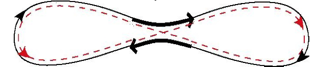
Figure 4: (color online) Sieber-Richter pair of orbits.

The first correction comes from the so-called Sieber-Richter pairs sieber ; sieber2 , see Fig. 4, which correspond to the factorization $\sigma=\pi^{-1}\rho$ with $\sigma=(12)(\bar{2}\bar{1})$, $\pi=(1\bar{2})(2\bar{1})$ and $\rho=(1\bar{1})(2\bar{2})$. The contribution this gives to $\mathcal{A}^{(0)}_{1,1}$ is $1/(i\pi\epsilon)$, which after applying $D_{1,1}$ leads to $i/(2\pi^{3}\epsilon^{2})$. However, this result vanishes after symmetrization (c.f. Eq.(20)) as exchanging $\epsilon_{1}$ and $\epsilon_{2}=\eta_{1}$ flips the sign of $\epsilon$. Also note that in this case symmetrization is equivalent to taking twice the real part. However, Sieber-Richter pairs give important contributions to the spectral form factor, defined as the Fourier transform

$$K(\tau)=\int_{-\infty}^{\infty}d\epsilon\,e^{i\epsilon\tau}\widetilde{\mathcal{R}}_{2}(\epsilon).$$ (47)

This apparent contradiction can be resolved as follows: The asymptotic behavior of the two-point correlation function can be written as a power series longb

$$\mathcal{R}_{2}(\epsilon)={\rm Re}\sum_{m=2}^{\infty}c_{m}\left(\frac{1}{i\epsilon}\right)^{m}+\ldots$$ (48)

where the dots represent oscillatory terms that we are neglecting in our present approach. The $m$-th term in this series expansion is associated to the terms proportional to $\tau^{m-1}$ in the spectral form factor. However the Fourier transform has to be carried out in the complex plane, requiring to take $\epsilon$ with a small imaginary increment that can then be sent to zero. Even powers of $\tau$ are thus associated to odd powers of $\frac{1}{i\epsilon}$ that would vanish after taking the real part but give a nonzero result if the increment is included. Our present approach could be extended to studying the asymptotics of the spectral form factor and its equivalents for higher-order correlation functions by incorporating such imaginary increments. However we will not carry out this generalization as our emphasis is on the correlation functions themselves.

The next order, with $L-V=2$, is associated with the appropriate factorizations of $(123)(\bar{3}\bar{2}\bar{1})$ and of $(12)(34)(\bar{4}\bar{3})(\bar{2}\bar{1})$. The former has four such factorizations, each contributing $z_{11}^{2}/(2\pi^{2})$ to $\mathcal{A}^{(0)}_{11}$. The latter has twenty such factorizations, each contributing $-z_{11}^{2}/(8\pi^{2})$. Hence, the contribution at this order to $\mathcal{A}^{(0)}_{1,1}$ is $-z_{11}^{2}/(2\pi^{2})$. After applying $D_{1,1}$ we get precisely $3/(2\pi^{4}\epsilon^{4})$, in agreement with RMT.

We have checked in the computer that at the next two orders, given by diagrams with $L-V=3$ and $L-V=4$, our semiclassical approximation also agrees with the corresponding RMT prediction. This is checking consistency with R2b ; R2c where the spectral form factor associated to the 2-point correlation function was treated to all orders.

VII.2 $3$-point function

As we have seen in Eq.(4), the correlation function $\mathcal{R}_{3}$ may be written as a sum containing $\widetilde{\mathcal{R}}_{0}=1$, $\widetilde{\mathcal{R}}_{2}$ and $\widetilde{\mathcal{R}}_{3}$. We have already discussed how the semiclassical approximation recovers the non-oscillatory part of $\widetilde{\mathcal{R}}_{2}$, so we only need to address the non-oscillatory part of $\widetilde{\mathcal{R}}_{3}$. RMT prediction for this, derivable from Eq.(8), is

$$\widetilde{\mathcal{R}}^{\rm no}_{3}={\rm Sym}_{3}\left[\frac{3}{2\pi^{6}}w_{12}^{2}w_{13}^{4}+\frac{1}{\pi^{6}}w_{12}^{3}w_{13}^{3}+\cdots\right],$$ (49)

where we have left out terms of higher order. Here we have set

$$w_{jk}=\frac{1}{\epsilon_{j}-\epsilon_{k}}.$$ (50)

We note that the indexing here is different from $z_{jk}=\frac{1}{\epsilon_{j}-\eta_{k}}$ due to $\eta_{k}=\epsilon_{J+k}$, Eq. (17), and it is more convenient for writing down our final results.

Remembering that $\widetilde{\mathcal{R}}_{3}=2{\rm Re}\widetilde{\mathcal{R}}_{1,2}$ (see Eq. (22)), we focus on $\widetilde{\mathcal{R}}_{1,2}$. Just as in the case of broken TRS, the leading order semiclassical contribution to this quantity should come from an orbit with a single $2$-encounter, correlated with two other orbits, see Fig. 2. However, as we have already seen this does not actually contribute anything because application of $D_{1,2}$ to a function that depends on only two variables returns zero.

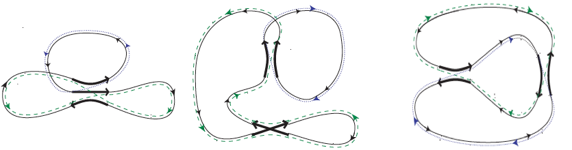
Figure 5: (color online) Diagrams contributing to $\widetilde{\mathcal{R}}_{12}$. There is one orbit, depicted by a full line, correlated with two others depicted by dashed lines. (Figure from the online appendix of longa .)

The second correction comes from the diagrams in Figure 5, having $L-V=2$. Without actually performing any calculations, we can see that their contributions to $\mathcal{A}^{(0)}_{1,2}$ are real, but after applying $D_{1,2}$ we arrive at an imaginary quantity. Since we need the real part of $\widetilde{\mathcal{R}}_{1,2}$, these diagrams do not contribute either.

	$\sigma$	$\pi$	$\rho=\pi\sigma$	mult.
(a)	$(1234)$	$(132\overline{4})$	$(1\overline{4}\overline{1})(2)$	6
(b)	$(1234)$	$(12\overline{3}\overline{4})$	$(1\overline{3}\overline{1})(3)$	3
(c)	$(1234)$	$(12\overline{4}\overline{3})$	$(1\overline{4})(24)$	2
(d)	$(1234)$	$(1\overline{2}3\overline{4})$	$(1\overline{1})(2\overline{4})$	2
(e)	$(123)(45)$	$(1245\overline{3})$	$(14\overline{3}\overline{1})(5)$	12
(f)	$(123)(45)$	$(1342\overline{5})$	$(1\overline{5}\overline{3}\overline{4})(3)$	8
(g)	$(123)(45)$	$(1452\overline{3})$	$(1\overline{3}\overline{5}\overline{1})(5)$	6
(h)	$(123)(45)$	$(125\overline{3}4)$	$(15)(2\overline{5}3)$	10
(i)	$(123)(45)$	$(134\overline{2}5)$	$(1\overline{4}24)(3)$	8
(j)	$(123)(45)$	$(134\overline{5}\overline{2})$	$(15\overline{5}\overline{3})(3)$	16
(k)	$(123)(45)$	$(142\overline{3}\overline{5})$	$(1\overline{3}\overline{4})(34)$	20
(l)	$(123)(45)$	$(14\overline{5}3\overline{2})$	$(1\overline{3})(34\overline{4})$	12
(m)	$(12)(34)(56)$	$(16\overline{2}345)$	$(1\overline{6}\overline{4}26)(4)$	192
(n)	$(12)(34)(56)$	$(164\overline{2}35)$	$(1\overline{4}26)(45)$	72
(o)	$(12)(34)(56)$	$(1\overline{2}\overline{6}345)$	$(1\overline{1}\overline{6}\overline{4}6)(4)$	96
(p)	$(12)(34)(56)$	$(1\overline{2}\overline{4}356)$	$(1\overline{1}\overline{4}45)(6)$	96
(q)	$(12)(34)(56)$	$(14\overline{6}\overline{2}35)$	$(16)(245\overline{4})$	72
(r)	$(12)(34)(56)$	$(14\overline{2}\overline{6}35)$	$(1\overline{4}6)(245)$	72
(s)	$(12)(34)(56)$	$(1\overline{2}6\overline{4}35)$	$(1\overline{1}6)(3\overline{6}\overline{3})$	96
(t)	$(12)(34)(56)$	$(1\overline{6}\overline{2}\overline{4}35)$	$(16)(2\overline{6}\overline{3}3)$	144

Table 3: Structures that contribute to $\widetilde{\mathcal{R}}_{12}$ and require TRS. See Table 1 for those not requiring TRS. The table omits structures whose contributions vanish after taking derivatives. It shows one representative cycle for each pair of cycles related by time reversal.

Finally, the diagrams responsible for the third correction have $L-V=3$. They include the ones shown in Figure 1 and Table 1, not requiring time-reversal symmetry. Table 3 shows the remaining 20 diagrams, which do require time-reversal symmetry. We are only displaying choices of permutations whose contributions do not vanish after taking derivatives. Note that the cycles of $\sigma$, $\pi$ and $\rho$ come in pairs related by time reversal; the table shows one representative cycle for each such pair. The contributions of these diagrams are all proportional to $z_{11}^{2}z_{12}+z_{11}z_{12}^{2}$. This has to be multiplied with the multiplicities as well as the factor

$$\frac{2^{J+K-V}}{\prod_{\ell}v_{\ell}!}\frac{(-1)^{L}}{(2\pi i)^{L-V}}$$ (51)

arising from Eqs. (38) and (45), leading to the overall result

$$\frac{1}{(i\pi)^{3}}(z_{11}^{2}z_{12}+z_{11}z_{12}^{2}).$$ (52)

After taking derivatives according to (40) we recover the desired correlation function given in (49). Here the factor 2 from (22) and the divisor $J!K!=2$ from (20) mutually cancel.

VII.3 4-point function

The non-oscillatory part of $\widetilde{\mathcal{R}}_{4}$ is predicted by RMT, according to Eq.(8), to be

$$\widetilde{\mathcal{R}}_{4}^{\rm no}={\rm Sym}_{4}\left[\frac{1}{8\pi^{4}}w_{12}^{2}w_{34}^{2}-\frac{3}{8\pi^{6}}w_{12}^{4}w_{34}^{2}\right]+\cdots,$$ (53)

where we included only terms up to order six. Note that ${\rm Sym}_{4}$ sums over all permutations of indices, including permutations that leave the argument unchanged.

The term of order four, $w_{12}^{2}w_{34}^{2}/\pi^{4}$, comes from the diagonal approximation, in which the orbits are identical (or mutually time reversed) two by two. This term involves factors $-\frac{1}{2\pi^{2}}w_{12}^{2}$ and $-\frac{1}{2\pi^{2}}w_{34}^{2}$ arising from the pairs according to (26), as well as a factor $\frac{1}{4}$ analogous to (20) and a factor 2 accounting for the two ways in which the $p$ and $q$ orbits can be paired.

It turns out that $\widetilde{\mathcal{R}}_{1,3}$ only contributes to $\widetilde{\mathcal{R}}_{4}$ with terms of order seven, so it doesn’t need to be considered in the context of the above prediction.

We still have to take into account $\widetilde{\mathcal{R}}_{2,2}$. This quantity allows for a partial diagonal approximation, see Eq.(II.4). This in fact reproduces the term of order six in (53). Here a factor $\frac{3}{4\pi^{2}}w_{12}^{4}$ arises from the pairs of orbits contributing to the term proportional to $\epsilon^{-4}$ in $\widetilde{\mathcal{R}}_{2}$, and the factor $-\frac{1}{2\pi^{2}}w_{34}^{2}$ accounts for coinciding or mutually time reversed orbits. The factor $\frac{1}{4}$ from (20) is compensated because for the two $p$ orbits we have two choices of which is included in the diagonal pair and which is included in the pair of orbits differing in encounters, and the same choice arises for the $q$ orbits.

	$\sigma$	$\pi$	$\rho=\pi\sigma$	mult.
(a)	$(123)$	$(13)(2)$	$(12)(3)$	1
(b)	$(12)(34)$	$(134)(2)$	$(123)(4)$	4
(c)	$(12)(34)$	$(1\overline{4})(2\overline{3})$	$(1\overline{3})(2\overline{4})$	1
(d)	$(12)(34)$	$(1\overline{2})(3\overline{4})$	$(1\overline{1})(3\overline{3})$	1

Table 4: Structures that contribute to $\widetilde{\mathcal{R}}_{22}$ for systems with TRS. Structures whose contributions vanish after taking derivatives are omitted. The table shows one representative cycle for each pair of cycles related by time reversal.

We are left with $\widetilde{\mathcal{R}}^{(0)}_{2,2}$, in which no two orbits are equal. The semiclassical approximation of order six is based on the diagrams in Table 4 where we have included only choices of permutations that give non-vanishing contributions after taking derivatives. However these are all proportional to $\sum_{j,j^{\prime},k,k^{\prime}}z_{jk}^{3}z_{j^{\prime}k^{\prime}}^{3}$ and thus vanish after symmetrization, as exchanging $\epsilon_{j}$ with $\eta_{k}$, or $\epsilon_{j^{\prime}}$ with $\eta_{k^{\prime}}$ flips the sign.

In conclusion, the semiclassical approximation to $\mathcal{R}_{4}$ agrees with the prediction from random matrix theory, up to the sixth order in perturbation theory.

We refer to the appendix for $\mathcal{R}_{5}$.

VIII Conclusions

We have developed a semiclassical approach that allows the calculation of the non-oscillatory terms of arbitrary spectral correlation functions of quantum chaotic systems. Using this approach, we have provided very strong evidence in favour of the Bohigas-Giannoni-Schmit conjecture that all local spectral statistics of such systems are described by those of random matrices taken from the appropriate Gaussian ensembles.

It still remains a challenge to show this agreement to all orders in perturbation theory. We believe it should be possible to adapt a powerful method originally introduced in the scattering context combinat5 ; combinat8 , based on using and explicitly evaluating some specific matrix integrals that encode the semiclassical approximation. Also the connection between semiclassics and the nonlinear sigma models of RMT R2c ; longb may provide useful insight.

Another problem still open is the semiclassical derivation of the oscillatory terms of the higher correlation functions. This is probably amenable to treatment using the theory developed here.

SM is grateful for support from the Leverhulme Trust Research Fellowship RF-2013-470. MN was supported by grants 303634/2015-4 and 400906/2016-3 from CNPq.

Appendix A 5-point function

We want to briefly discuss the diagrams relevant for the 5-point correlation function, both for systems with and without TRS.

A.1 Broken TRS

The 5-point function is determined by diagrams with $J=1$, $K=4$ as well as $J=2$, $K=3$ (which are trivially related to the diagrams where $J$ and $K$ are swapped). In either case there are no contributing diagrams for $L-V=1$ or $2$. For $L-V=3$ we obtain a large number of diagrams which are omitted here. However their contributions to $\mathcal{A}_{2,3}^{(0)}$ all vanish upon differentiation and/or they include one factor $w_{jk}$ whose indices do not appear in any of the other factors. Upon taking derivatives this factor appears cubed. It then vanishes after symmetrization as it is odd under exchanging indices. As $L-V=3$ corresponds to the 8th order in $w_{jk}$ this shows that all off-diagonal contributions up to this order vanish. The partial diagonal contributions vanish as well as they are based on off-diagonal contributions to $\widetilde{\mathcal{R}}_{3}$ which have already been shown to give zero. As desired this leaves only the diagonal approximation.

A.2 Preserved TRS

For time-reversal symmetric systems the RMT prediction (in leading order) can be brought to the form

$$\widetilde{\mathcal{R}}_{5}^{\rm no}={\rm Sym}_{5}\left[-\frac{3}{4\pi^{8}}w_{12}^{2}w_{13}^{4}w_{45}^{2}-\frac{1}{2\pi^{8}}w_{12}^{3}w_{13}^{3}w_{45}^{2}\right]+\cdots.$$ (54)

Again all exclusively off-diagonal contributions up to 8th order in $w_{jk}$ vanish. For $J=1$, $K=4$ the situation is exactly as without TRS, and there are no additional diagrams requiring TRS. For $J=2$, $K=3$ there is one additional diagram with $L-V=2$ and two structures including $\sigma=(12)(34)$, $\pi=(1\overline{2})(34)$, $\rho=(1\overline{1})(3)(4)$. However their contributions vanish after taking derivatives. For $L-V=3$ there are also further diagrams, but their contributions all vanish due to either of the reasons discussed for broken TRS.

The contribution in (54) arises from the leading partial diagonal term. Here three orbits are arranged according to one of the diagrams contributing to $\widetilde{\mathcal{R}}_{3}$, and two orbits coincide up to time reversal. If the indices 1,2,3 are associated to the former orbits and 4, 5 to the latter orbits our previous results (26) and (49) entail factors $\frac{3}{2\pi^{6}}w_{12}^{2}w_{13}^{4}+\frac{1}{\pi^{6}}w_{12}^{3}w_{13}$ and $-\frac{1}{2\pi^{2}}w_{45}^{2}$ multiplying to (54). There are further combinatorial factors but they cancel (a 2 to remove the $\frac{1}{2}$ from (20) included in the first factor, $\frac{1}{J!K!}=\frac{1}{12}$ as the factor from (20) arising in the present case, 2 choices to select the $p$ orbit contributing to the diagonal approximation, and 3 choices for the $q$ orbit).

References

- (1) O. Bohigas, M.J. Giannoni and C. Schmit, Phys. Rev. Lett. 52, 1 (1984);
- (2) G. Casati, F. Valz-Gris and I. Guarneri, Lett. Nuovo Cimento 28, 279 (1980).
- (3) M.V. Berry, Ann. Phys. (N.Y.) 131, 163 (1981).
- (4) F. Haake, Quantum Signatures of Chaos (Springer, 2001).
- (5) M. Gutzwiller, Chaos in Classical and Quantum Mechanics (Springer, New York, 1990).
- (6) J. H. Hannay and A. M. Ozorio de Almeida, J. Phys. A 17, 3429 (1984).
- (7) M.V. Berry, Proc. R. Soc. London A 400, 229 (1985).
- (8) N. Argaman, F. M. Dittes, E. Doron, J. P. Keating, A. Yu. Kitaev, M. Sieber, and U. Smilansky, Phys. Rev. Lett. 71, 4326 (1993).
- (9) M. Sieber and K. Richter, Phys. Scr., T 90, 128 (2001).
- (10) M. Sieber, J. Phys. A 35, L613 (2002).
- (11) S. Heusler, S. Müller, P. Braun, and F. Haake, J. Phys. A 37, L31 (2004).
- (12) S. Müller, S. Heusler, P. Braun, F. Haake, and A. Altland, Phys. Rev. Lett. 93, 014103 (2004).
- (13) S. Müller, S. Heusler, P. Braun, F. Haake, and A. Altland, Phys. Rev. E 72, 046207 (2005).
- (14) S. Heusler, S. Müller, A. Altland, P. Braun, and F. Haake, Phys. Rev. Lett. 98, 044103 (2007).
- (15) J. P. Keating and S. Müller, Proc. R. Soc. Lond. A 463, 3241 (2007).
- (16) S. Müller, S. Heusler, A. Altland, P. Braun and F. Haake, New J. Phys. 11, 103025 (2009).
- (17) T. Nagao and S. Müller, J. Phys. A 42, 375102 (2009).
- (18) P. Shukla, Phys. Rev. E 55, 3886 (1997).
- (19) G. Berkolaiko, J.M. Harrison and M. Novaes, J. Phys. A 41, 365102 (2008).
- (20) G. Berkolaiko and J. Kuipers, New J. Phys. 13, 063020 (2011).
- (21) M. Novaes, Europhys. Lett. 98, 20006 (2012).
- (22) G. Berkolaiko and J. Kuipers, Phys. Rev. E 85, 045201 (2012).
- (23) G. Berkolaiko and J. Kuipers, J. Math. Phys. 54, 112103 (2013).
- (24) G. Berkolaiko and J. Kuipers, J. Math. Phys. 54, 123505 (2013).
- (25) M. Novaes, J. Phys. A 46, 095101 (2013).
- (26) M. Novaes, Ann. Phys. 361, 51 (2015).
- (27) M. Novaes. J. Math. Phys. 56, 062109 (2015).
- (28) M. Novaes. J. Math. Phys. 57, 122105 (2016).
- (29) Z. Pluhar and H. A. Weidenmüller, Phys. Rev. Lett. 112, 144102 (2014).
- (30) Z. Pluhar and H. A. Weidenmüller, J. Phys. A 48, 275102 (2015).
- (31) M.L. Mehta, Random Matrices (Academic Press, 2004).
- (32) P. Forrester, Log-gases and random matrices (Princeton University Press, 2010).
- (33) E. Brézin and S. Hikami, J. Phys. A 36, 711 (2003).
- (34) E. Kanzieper, Phys. Rev. Lett. 89, 250201 (2002).
- (35) S. Müller, S. Heusler, P. Braun, and F. Haake, New J. Phys. 9, 12 (2007).
- (36) S. Müller and M. Sieber, Chapter 33 of The Oxford Handbook of Random Matrix Theory eds. G. Akemann, J. Baik, and P. Di Francesco (Oxford University Press, 2011)
- (37) M. Turek and K. Richter, J. Phys. A 36, L455 (2003)
- (38) D. Spehner, J. Phys. A 36, 7269 (2003).