First passage under restart with branching

Abstract

First passage under restart with branching is proposed as a generalization of first passage under restart. Strong motivation to study this generalization comes from the observation that restart with branching can expedite the completion of processes that cannot be expedited with simple restart; yet a sharp and quantitative formulation of this statement is still lacking. We develop a comprehensive theory of first passage under restart with branching. This reveals that two widely applied measures of statistical dispersion—the coefficient of variation and the Gini index—come together to determine how restart with branching affects the mean completion time of an arbitrary stochastic process. The universality of this result is demonstrated and its connection to extreme value theory is also pointed out and explored.

Restart can expedite the completion of a myriad of processes Restart1 ; Restart2 ; Restart3 ; Restart-Biophysics1 ; Restart-Biophysics2 ; Restart-Biophysics3 ; Restart4 ; Restart5 ; ReuveniPRL ; PalReuveniPRL ; Restart-Search1 ; Restart-Search2 ; Restart-Search3 . It works by taking advantage of stochastic fluctuations to trade long completion times with ones which are shorter on average. Thus, restart is particularly effective in expediting processes whose statistical completion time distributions are very broad. A classical example of this principle is the first passage time (FPT) FPT1 ; FPT2 to a stationary target of a particle undergoing diffusion RednerBook ; MetzlerBook ; Schehr-review . The distribution of this FPT is so broad that its mean diverges RednerBook . On average, a diffusive particle will thus take an infinite amount of time to reach a target; but restart can change this situation dramatically. Indeed, stopping the particle’s motion intermittently and placing it back at the origin to continue its motion from there regularizes the FPT distribution and renders its mean finite Restart1 ; Restart2 . Remarkably, this ‘regularization by restart’ works for any process with divergent mean completion times – regardless of the specific details Restart-Biophysics1 ; Restart-Biophysics2 ; ReuveniPRL ; PalReuveniPRL .

Some processes cannot be expedited with restart as this strategy crucially depends on the existence of stochastic fluctuations in completion times. Consider, as an illustrative example, a train which travels from point A to B at a constant velocity. Aside from small glitches here and there, such train takes a fixed amount of time to reach its final destination. Thus, the train’s FPT distribution is very sharply peaked around its mode. As it turns out, this punctuality is intimately related with the fact that taking the train, at any point along its route, and placing it back at the dock of departure will only prolong its journey. Indeed, whenever the coefficient of variation ($CV$) of the completion time is smaller than one – applying restart will increase the mean completion time Restart-Biophysics1 ; Restart-Biophysics2 ; ReuveniPRL ; PalReuveniPRL . As the $CV$ is the ratio of the standard deviation to the mean, this criterion captures the need for relatively large stochastic fluctuations; also, this criterion sets a sharp boundary for the application of restart as a ‘speed-up’ mechanism.

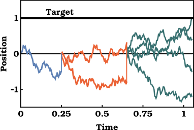
Figure 1: An illustration of diffusion under restart with branching. When restart occurs, particles are brought back to the origin and each particle is branched into two identical copies of itself.

Branching a process – so as to create several competing copies of it that run parallel to one another – is a different ‘speed-up’ strategy that is used, e.g., in computer science parallel-processing1 ; parallel-processing2 . Branching allows one to reduce the time taken to solve a problem at the expense of resource investment. Restart is also used for that purpose restart-CS1 ; restart-CS2 , and while it is not always applicable it could generate speedup without requiring additional resources. A strategy that combines restart and branching may thus allow one to have the best of both worlds.

Branching was extensively studied, e.g., in birth and death processes Harris-Book , reaction-diffusion systems Bramson ; Derrida , Brownian motion Kabir-1 ; Kabir-2 , and epidemic spread Satya-PNAS . However, it was just earlier this year that branching was considered in the context of restart—coining the term ‘branching search’ Iddo-Branch . To illustrate this, envision a scout that is dispatched by a central command to search for a hidden target, e.g., treasure, an enemy base, or a group of missing people. If the scout fails to find the target within a certain time window then central command calls the scout back, and dispatches two new scouts to the task. If the two also fail within a certain time window then they are also called back, and four new scouts are dispatched to the task. Thus, instead of merely resetting the search in an attempt to expedite it, efforts to locate the target are doubled with every failed attempt.

A scenario of the type described above could be mathematically modeled by, e.g., considering diffusion under stochastic restart with branching (Fig. 1); yet this model does not fall under the existing theoretical framework. Moreover, while our understanding of first-passage under restart enjoys the aforementioned $CV$ criterion, a universal criterion that determines the effect of ‘restart-&-branching’ on the mean completion time of a general stochastic process is currently missing. Indeed, while the great advantages that restart brings to existing search strategies Shlesinger ; Benichou-review were already discussed extensively Restart1 ; Restart-Biophysics2 ; PalReuveniPRL ; Restart-Search2 ; Restart-Search3 ; Search-DNA ; Chechkin , the exploration of ’branching search’ Iddo-Branch has just begun—determining the combined effect of restart and branching is a non-trivial task even for the relatively simple case illustrated in Fig. 1.

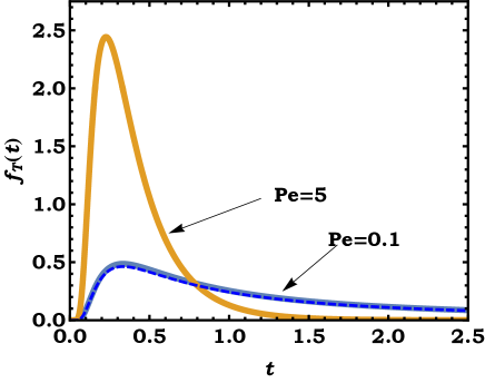
Figure S1: The Inverse-Gaussian first passage time distribution for diffusion with drift is plotted for two different values of the Péclet number (solid lines). Here, we fixed $L/D=2.0$ so that $Pe=V$. It can be seen that when $Pe=5$ the corresponding distribution is already sharply peaked around its mode. On the other extreme, when $Pe=0.1$, the corresponding distribution closely resembles the one which is obtained in the pure diffusion limit (dashed line).

Diffusion under restart with branching.—Consider a particle undergoing diffusion with drift. The particle starts its motion at the origin and drift-diffuses at an average velocity $V>0$ until it hits a target located at $L>0$. This will happen at a random time $T$ which comes from the Inverse-Gaussian distribution $f_{T}(t)=\frac{L}{\sqrt{4\pi Dt^{3}}}e^{-\frac{(L-Vt)^{2}}{4Dt}}(t\geq 0)$, with $D$ standing for the diffusion coefficient Cox-Miller-Book . Defining the Péclet number $Pe=LV/2D$, one can then trivially observe that diffusion (drift) becomes negligible in the limit of $Pe\gg 1$ ($Pe\ll 1$). Indeed, $f_{T}(t)$ becomes sharply peaked for high Péclet numbers and resembles that of a particle undergoing pure diffusion when Péclet numbers are low (Fig. S1). Thus, by tuning the Péclet number, one can explore the wide range of cases that stand between the two extreme scenarios discussed above: simple motion at a constant velocity and pure diffusion.

Let us now consider the above process, but with the addition of restart and branching (Fig. 1). Specifically, assume that restart can occur with some probability at any given point in time; and that when this happens our particle is taken back to the origin and branched into two, or generally $m$, identical particles. These particles will start their motion anew, but if restart occurs again they will all be taken back to the origin and branched as before. This procedure repeats itself until one of the particles in the system hits the target.

To study the effect of restart with branching, we simulated the process illustrated in Fig. 1 SM . First, we wanted to explore what happens when restart with branching is introduced into the system. Letting $r$ denote the constant rate at which restart with branching occurs, we looked at the logarithmic derivative of the mean FPT to the target with respect to $r$ at $r=0$. This was plotted vs. the Péclet number for different values of the branching parameter $m$ (Fig. 2, markers). A negative derivative indicates that the introduction of restart with branching will, on average, expedite first passage to the target, and the converse is true when a positive derivative is found. Results coming from simulations were later on corroborated by the general theory developed below (Fig. 2, dashed lines).

Analyzing the results presented in Fig. 2, we would first like to draw attention to the case $m=1$. In this degenerate case restart is not accompanied by branching and one can observe that the derivative changes sign exactly when $Pe=1$. This is no surprise. The mean of the Inverse-Gaussian distribution above is $L/V$ and its standard deviation is $\sqrt{2DL/V^{3}}$. Letting $CV$ stand for the coefficient of variation of this distribution, we observe that $CV^{2}=1/Pe$. Recalling that the theory of first passage under restart asserts that restart will expedite the completion of a process if and only if $CV>1$ Restart-Biophysics1 ; Restart-Biophysics2 ; ReuveniPRL ; PalReuveniPRL , we conclude that the observed behaviour is a special case of a more general one.

For $m>1$, we see that the critical Péclet number at which the derivative changes sign is always larger than unity. Moreover, this critical number grows as $m$ increases. Thus, in the case of diffusion with drift, branching allows restart to reduce the mean FPT even when the underlying FPT distribution is much narrower than the critical limit for simple restart ($Pe=1$). However, and in contrast to the $m=1$ case, we find the corresponding set of critical $CV$s (Fig. S2) to be particular to diffusion with drift, i.e., non-universal. Any general characterization of the effect that restart with branching has on the mean completion time of a generic process must thus rely on more than the first two moments of the underlying time distribution. To find this characterization, and further deepen our understanding, we now develop a general theory of first passage under restart with branching.

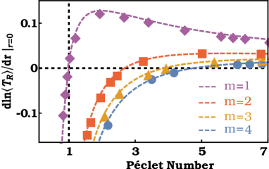
Figure 2: The effect the introduction of restart with branching has on the mean FPT (to a stationary target) of a particle undergoing diffusion with drift. Results are shown for different values of the Péclet number, $Pe=LV/2D$, and branching index $m$.

A theory of first passage under restart with branching.—Consider a generic process that starts at time zero and, if allowed to take place without interruptions, completes after a random time $T$. The process, however, can also be restarted after some random time $R$ and consecutively branched into $m$ daughter processes which are independent and identical copies of the parent process $(m=1,2,3,\cdots)$. Thus, if restart prevents the parent process from completing, $m$ daughter processes will start in its stead. The same procedure will then repeat itself: if one of the daughter processes is able to finish prior to restart completion will be declared. Otherwise, following a second restart event, each daughter process will, in itself, be branched into $m$ processes that will once again start their course afresh; and so on and so forth until one of the offspring processes is able to complete (Fig. 3).

To analyze the above scenario, we let $R^{\prime}$ and $\{T_{1},\cdots,T_{m}\}$ denote independent and identically distributed copies of $R$ and $T$ respectively. We then observe that $T_{R}$—the random completion time of a generic process under restart with branching—can be written as

$$\begin{array}[]{l}T_{R}=\left\{\begin{array}[]{lll}T&&\text{if }T<R\text{ }\\ &\text{ \ \ }\\ R+[T^{(m)}]_{R^{\prime}}&&\text{if }R\leq T\text{ ,}\end{array}\right.\text{ }\end{array}$$ (1)

with $T^{(m)}=\text{min}\{T_{1},\cdots,T_{m}\}$. The rational leading to Eq. (1) is simple. If the parent process is able to complete prior to restart the process there ends and $T_{R}=T$. Otherwise, after some random time $R$, restart with branching occurs. One could then ‘virtually’ join all the newly formed daughter processes into a single process whose uninterrupted completion time is $T^{(m)}$, i.e., the minimum over $m$ IID copies of $T$. However, since this joint process is also subject to restart with branching its actual completion time is given by $[T^{(m)}]_{R^{\prime}}$. Thus, when restart precedes completion, we have $T_{R}=R+[T^{(m)}]_{R^{\prime}}$.

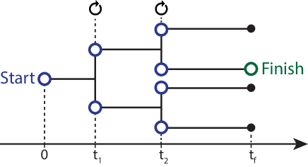
Figure 3: An illustration of first passage under restart with branching ($m=2$). Restart and branching takes place at time $t_{1}$ and thereafter at time $t_{2}$. Completion takes place at time $t_{f}$.

Eq. (1) can be used to derive a formula for the mean FPT of a process that has been subjected to restart with branching. This is done in iterative steps. First, observe that Eq. (1) implies that $T_{R}=\text{min}(T,R)+I(R\leq T)[T^{(m)}]_{R^{\prime}}$, where $\text{min}(T,R)$ is the minimum of $T$ and $R$, and $I(R\leq T)$ is an indicator random variable which takes the value one when $R\leq T$ and zero otherwise. Taking expectations, and utilizing statistical independence, we obtain that

$$\langle T_{R}\rangle=\langle\text{min}(T,R)\rangle+\text{Pr}(R\leq T)~{}\langle[T^{(m)}]_{R}\rangle\text{ .}$$ (2)

The first term in Eq. (2) and the probability that $R\leq T$ can then be evaluated given the distribution functions of $T$ and $R$ SM . To further proceed, we utilize Eq. (1) one more time to obtain $[T^{(m)}]_{R}=\text{min}(T^{(m)},R)+I(R\leq T^{(m)})[T^{(m^{2})}]_{R^{\prime}}$ SM . Taking expectations one arrives at an equation similar to Eq. (2) SM where $\text{min}(T^{(m)},R)$ and the probability that $R\leq T^{(m)}$ can once again be directly computed given the distribution functions of $T$ and $R$. As for the expectation of $[T^{(m^{2})}]_{R^{\prime}}$, this is again evaluated by iterative use of Eq. (2).

Carried ad infinitum, the above procedure yields a formula that allows the evaluation of $\langle T_{R}\rangle$ for arbitrary choices of $T$ and $R$ SM . Of particular interest in that regard is the case where restart is conducted at a constant rate $r$, i.e., when the random restart time $R$ is exponentially distributed with mean $1/r$ Restart1 ; Restart2 ; Restart-Biophysics1 ; Restart-Biophysics2 ; ReuveniPRL . We then find

$$\langle T_{R}\rangle=\frac{1}{r}~{}\sum_{n=0}^{\infty}~{}\prod_{k=0}^{n}~{}[1-\tilde{T}^{(m^{k})}(r)]~{},$$ (3)

with $\tilde{T}^{(m^{k})}(r)$ standing for the Laplace transform of $T^{(m^{k})}$ evaluated at $r$ SM . Equation (3) allows one to study the effect of restart with branching on the mean completion times of various process by systematic evaluation of $\langle T_{R}\rangle$ (Fig. 4). Depending on the process, and the branching index $m$, the introduction of restart with branching could then either increase or decrease the mean completion time. A universal and clear cut criterion to determine which of the two occurs is therefore in need. We will now derive this criterion and show that aside from the coefficient of variation it is also sensitive to another measure of statistical dispersion: the generalized Gini index.

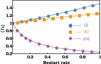
Figure 4: Mean FPT under restart with branching vs. restart rate for different FPT processes: (i) cover time of a random walker Benichou-covertime ; (ii) diffusion with drift Cox-Miller-Book ; and (iii) an infectious cells growth model Iyer-Biswas . In all three cases, the branching index was set to $m=2$, and time was measured in units of the mean FPT in the absence of restart and branching. Dashed lines are theoretical curves computed based on Eq. (3) and markers come from Monte Carlo simulations (SM ).

The Gini index is widely applied in economics and in the social sciences as a measure of socioeconomic inequality Gini-methodology . In general, the Gini index is a measure of statistical dispersion that is applicable to non-negative valued random variables with positive means Iddo-Tour . Here we apply the Gini index in the context of the random variable $T$. The Gini index has several equivalent representations, and one of them is Iddo-Tour $GI=1-\langle\min\left\{T_{1},T_{2}\right\}\rangle/\langle T\rangle$, where $T_{1},T_{2}$ are two IID copies of $T$. In turn, this representation can be generalized from two IID copies of $T$ to $m$ copies, $\{T_{1},\cdots,T_{m}\}$, yielding the following generalized Gini index Iddo-Physica

$$GI_{m}=1-\langle\min\left\{T_{1},\cdots,T_{m}\right\}\rangle/\langle T\rangle\text{ ,}$$ (4)

$(m=1,2,...)$. Note that the index of order one vanishes $GI_{1}=0$; and that the index of order two is the Gini index $GI_{2}=GI$.

With the generalized Gini index at hand, and the coefficient of variation $CV=\sigma(T)/\langle T\rangle$, we find that $\frac{d\langle T_{R}\rangle}{dr}|_{r=0}<0$ if and only if SM

$$CV^{2}+2\cdot{GI}_{m}>~{}1\text{ .}$$ (5)

Equation (5) provides a universal criterion that determines how restart with branching affects the mean completion time of an arbitrary stochastic process. When $m=1$, i.e., when there is no branching, Eq. (5) boils down to the known ‘pure restart’ criterion $CV>1$ Restart-Biophysics1 ; Restart-Biophysics2 ; ReuveniPRL ; PalReuveniPRL . However, for $m>1$, we see that the criterion in Eq. (5) also depends on the generalized Gini Index. To better illustrate this we now consider a concrete example.

Consider the Weibull distribution $\text{Pr}[T\geq t]=e^{-(t/\alpha)^{\beta}}~{}(t\geq 0)$; with $\alpha,\beta>0$ standing respectively for the scale and shape parameters. The coefficient of variation of this distribution is known to be given by $CV^{2}=\Gamma(1+2/\beta)/\Gamma(1+1/\beta)^{2}-1$, where $\Gamma(x)$ is the Gamma function. To compute $GI_{m}$, we first observe that if $T$ is a Weibull random variable with parameters $\alpha$ and $\beta$, then $T^{(m)}=\min\left\{T_{1},\cdots,T_{m}\right\}$ is also a Weibull random variable with scale parameter $\alpha/m^{1/\beta}$ and shape parameter $\beta$ SM . Eq. (4) then gives ${GI}_{m}=1-{m^{-1/\beta}}$. Both $CV^{2}$ and ${GI}_{m}$ are then uniquely determined by the shape parameter which provides a simple handle on the dispersion of the Weibull distribution—the larger $\beta$ the smaller $CV^{2}$ and ${GI}_{m}$. The criterion in Eq. (5) can then be explored graphically (Fig. 5) and also written explicitly to read $m>\big{[}2\Gamma(1+1/\beta)^{2}/\Gamma(1+2/\beta)\big{]}^{\beta}\text{ .}$ This inequality relates the branching index $m$ to the shape parameter $\beta$ and provides a simple test to determine the effect of restart with branching. In particular, note that for $\beta<1$, a.k.a. the stretched exponential regime SEx1 ; SEx2 , this condition is always satisfied (Fig. 5 left). In SM we demonstrate that explicit forms of Eq. (5) can also be attained for distributions other than the Weibull, e.g., the uniform and Pareto.

Discussion.—The universal criterion in Eq. (5) can be re-written in the form

$$\frac{1}{2}\langle T^{2}\rangle/\langle T\rangle>\langle\text{min}\{T_{1},\cdots,T_{m}\}\rangle~{}.$$ (6)

This form has a probabilistic interpretation which becomes evident when contrasting two possible scenarios. Consider first a process (with no restart) that repeats itself indefinitely a-la Sisyphus. Renewal theory then asserts that if this process is probed at an arbitrary time epoch, $\frac{1}{2}\langle T^{2}\rangle/\langle T\rangle$ units of time will pass, on average, before the next completion event is observed Gallager . Now consider the introduction of an infinitesimally small restart rate. Properties of the Poisson process then assert that restart will occur at an arbitrary moment in time, thus replacing an expected mean completion time of $\frac{1}{2}\langle T^{2}\rangle/\langle T\rangle$ pre-restart by $\langle\text{min}\{T_{1},\cdots,T_{m}\}\rangle$ post-restart. Comparing the two alternatives, Eq. (5) follows immediately.

Equation (6) invites a connection to the fundamental theorem of Extreme Value Theory (EVT), which pinpoints the universal limit-laws of the maxima and minima of IID random variables: Gumbel, Fréchet, or Weibull. In our case, considering a linear scaling of the minimum appearing on the right-hand side of Eq. (6), we arrive at the Weibull limit-law. Hence, for $m\gg 1$, the minimum is approximated (in law) by $W/s_{m}$, where $s_{m}$ is a scaling parameter that satisfies $\underset{m\to\infty}{\lim}s_{m}=\infty$, and where $W$ is a Weibull-distributed limiting random variable SM . Consequently, the right-hand side of Eq. (6) can be approximated by $\langle W\rangle/s_{m}$ – thus establishing an asymptotic version of the criterion in Eq. (6).

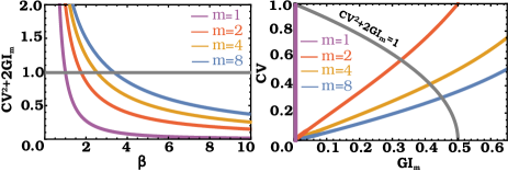
Figure 5: Graphical exploration of the criterion from Eq. (5) when applied to the Weibull distribution. Left. $CV^{2}+2{GI}_{m}$ is plotted vs. the shape parameter $\beta$ for different values of the branching index $m$. Right. The $CV$ is plotted vs. $GI_{m}$ for different values of the branching index $m$. In both panels, the $CV^{2}+2{GI}_{m}=1$ line separates the two different behavioural phases that are predicted by Eq. (5).

Equation (5) can also be expressed in terms of two equality indices. The first equality index is based on the coefficient of variation, and is given by $\mathcal{R}_{2}=1/(1+CV^{2})$; this index belongs to a continuum of equality indices that are intimately related to the Renyi entropy RenEq . The second equality index is the counterpart of the generalized Gini index of Eq. (4), and is given by $\mathcal{G}_{m}=1-{GI}_{m}$; this index belongs to a continuum of equality indices that extend the Gini index Iddo-Physica . In terms of these two equality indices, Eq. (5) admits the following product representation

$$\mathcal{R}_{2}\cdot\mathcal{G}_{m}<\frac{1}{2}\text{ .}$$ (7)

Interestingly, Eq. (7) resembles an uncertainty principle which provides a fundamental bound on $\mathcal{G}_{m}$ given $\mathcal{R}_{2}$ and vice versa. Indeed, if the introduction of an infinitesimally small restart rate is observed to expedite the completion of a given process: $\mathcal{G}_{m}$ cannot exceed $\frac{1}{2}\mathcal{R}^{-1}_{2}$. Thus, high equality (less uncertainty) of one measure must be compensated by low equality (more uncertainty) of the other.

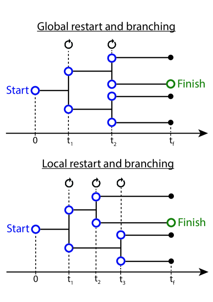
Figure S3: Global vs. local restart and branching.

Conclusions.—Restart has recently attracted considerable attention Restart1 ; Restart2 ; Restart3 ; Restart4 ; Restart5 ; ReuveniPRL ; PalReuveniPRL ; Restart-Search1 ; Restart-Search2 ; Restart-Search3 ; Iddo-Branch ; restart_conc1 ; restart_conc2 ; restart_conc3 ; restart_conc4 ; restart_conc5 ; restart_conc6 ; restart_conc7 ; restart_conc8 ; restart_conc9 ; restart_conc10 ; restart_conc11 ; restart_conc12 ; restart_conc13 ; restart_conc14 ; restart_conc15 ; restart_conc16 ; restart_conc17 ; restart_conc18 ; restart_conc19 ; restart_conc20 ; restart_conc21 touching on subjects ranging from stochastic thermodynamics restart_thermo1 ; restart_thermo2 to optimization theory Optimization , and from quantum mechanics Quantum1 ; Quantum2 to biological physics Restart-Biophysics1 ; Restart-Biophysics2 ; Restart-Biophysics3 ; Restart-Biophysics4 . In this letter we extended the theory of first passage under restart to include branching, and provided a universal criterion to determine the effect that restart with branching has on a general FPT process. Throughout this letter it was assumed that restart is global, i.e., that there is one central timer that sets the restart-&-branching epochs for all the active processes. However, situations where restart is local, i.e., each FPT process has its own internal timer for restart-&-branching (Fig. S3), could also arise and are as important.

Consider, for example, the spread of an epidemic within a large population of agents (humans, computers, etc.). There, one may be interested in the time it takes for a specific target agent to become infected. The epidemic initiates from an arbitrary agent, ‘patient zero’. Then, two scenarios can take place: patient zero either infects the target agent before it infects some other agent, or vice versa. The first scenario ends the process. The second scenario generates two infected agents, each proceeding independently the ‘hunt’ for the target agent. Thus, we obtain first passage under local restart-&-branching (with $m=2$).

Evidently, global and local restart-&-branching are inherently different. Nonetheless, we show that Eqs. (5-7) are not sensitive to this difference SM . Namely, the novel universal criterion established in this letter — to determine the effect of restart-&-branching on mean completion times — applies regardless of whether restart is global or local.

Acknowledgments.—We thank Dr. Somrita Ray and Dr. Debasish Mondal for commenting on early versions of this manuscript. A.P. acknowledges support from the Raymond and Beverly Sackler Post-Doctoral Scholarship. S.R. acknowledges support from the Azrieli Foundation.

Supplementary Material for First Passage Under Restart with Branching

SI Supplementary figures

Figure S2: Critical $CV$s, as obtained in Fig. 2 from the relation $CV^{2}=1/Pe$, vs. the branching index $m$ for diffusion with drift under restart with branching. As $m$ increases, lower $CV$s are found indicating that restart with branching can expedite completion even if first passage time distributions are narrow ($CV<1$). However, while the critical $CV$ value found for $m=1$ is universal (true for any process), the ones found for $m>1$ are particular to diffusion with drift.

SII Supplementary text

SII.1 Details of the simulations in Fig. 2 and Fig. 4

In this subsection, we provide details of simulations done in Fig. 2 and Fig. 4. These were carried out using the following methodology. Based on the process at hand (see details below), we determined the distribution of the random completion time $T$ in the absence of restart and branching. Then, we set the distribution of the restart time $R$ to be exponential with mean $1/r$ (note, again, that this is equivalent to setting a constant restart rate $r$). After these distributions have been set, we simply followed Eq. (1) to gather statistics about the completion time of the process when it is subjected to restart with branching. This was done using the following algorithm: (i) draw two random numbers from the respective distributions of $T$ and $R$; (ii) If $T<R$, set the completion time $T_{R}$ to $T$ and end the program; (iii) Otherwise, when $R\leq T$, record the time $R$ that has passed, restart the parent process and branch it into $m$ daughter processes that are identical to it; (iv) Set $T_{R}=R+[T^{(m)}]_{R^{\prime}}$, where $T^{(m)}$ is a random variable distributed like the minimum of $m$ copies of $T$, and $R^{\prime}$ is a random restart time taken from the same distribution as $R$; (v) Repeat steps (i)-(iv) with $T^{(m)}$ substituting for $T$ to determine $[T^{(m)}]_{R^{\prime}}$ and consecutively $T_{R}$. (vi) Repeat steps (i)-(v) many times to gather multiple samples of the random variable $T_{R}$. Use these to compute $\langle T_{R}\rangle$—the mean completion time of the process when subjected to restart with branching. Actual implementation of the above algorithm depends on the exact distribution of the random variable $T$ and on the value of the branching index $m$ used. These are specified below.

• Fig. 2 — To study the effect that the introduction of an infinitesimally small restart rate has on the mean FPT of a particle undergoing diffusion with drift, we simulated the process illustrated in Fig. 1 in the main text. For this, we let the random time $T$ come from the inverse Gaussian distribution sm-Cox-Miller-Book

  $$f_{T}(t)=\frac{L}{\sqrt{4\pi Dt^{3}}}e^{-\frac{(L-Vt)^{2}}{4Dt}}~{}(t\geq 0).$$ (S1)

  Parameter values were set to: $D=0.5$ and $L=1.0$; and the value of $V$ was set to obey $Pe=LV/2D$. The value of the branching index was varied in the range $m={1,2,3,4}$.

• Fig. 4: Cover time of a random walker — Here, we let the random time $T$ be the normalized cover time of a random walker on a network of $N$ sites. The cover time $\mathcal{T}(N)$ is defined as the time needed by the walker to visit all sites in the network. In sm-Benichou-covertime , the authors showed that after proper scaling this cover time admits a universal limit law. More specifically, letting $\langle\tau\rangle$ denote the global mean first passage time, defined as the mean first-passage time to a given target site averaged over all starting sites, it was shown that $X=\mathcal{T}/\langle\tau\rangle-\ln N$ converges to the following asymptotic distribution

  $$f_{X}(x)=\exp\left(-x-e^{-x}\right)~{}(-\infty\leq x\leq\infty),$$ (S2)

  in the limit of $N\to\infty$. Setting

  $$T=\langle\tau\rangle\cdot[X+\ln N]/\langle\mathcal{T}\rangle=\mathcal{T}/\langle\mathcal{T}\rangle,$$ (S3)

  with $N=10^{4}$ and $\langle\tau\rangle=4.1$, we generated samples from the random variable $T$ by drawing a random number from the distribution of $X$ in Eq. (S2) and then substituting it back in Eq. (S3).
  

• Fig. 4: Diffusion with drift — Here we once again let the random time $T$ come from the inverse Gaussian distribution sm-Cox-Miller-Book

  $$f_{T}(t)=\frac{L}{\sqrt{4\pi Dt^{3}}}e^{-\frac{(L-Vt)^{2}}{4Dt}}~{}(t\geq 0).$$ (S4)

  Parameters values were taken such that $L^{2}/2D=10.0$ and $L/V=1.0$ thus setting $\langle T\rangle=1.$
  

• Fig. 4: Cell growth model — Here we let the random time $T$ come from the Gamma distribution

  $$f_{T}(t)=\frac{\kappa e^{-\kappa t}(\kappa t)^{-1+\theta}}{\Gamma(\theta)}~{}(t\geq 0).$$ (S5)

  Parameter values were set to $\kappa=\theta=1/9$ so that $\langle T\rangle=\theta/\kappa=1$. In sm-Iyer-Biswas this distribution was used to describe the time it takes a cell growing at a rate $\kappa$ to reach a certain threshold size $\theta$.

SII.2 Detailed derivation of Eq. (3)

Here we provide a detailed derivation of Eq. (3) in the main text. We start by letting ${R^{\prime},R^{\prime\prime},R^{\prime\prime\prime}...}$ denote independent and identically distributed copies of the random restart time $R$. Iterative use of Eq. (1) in the main text then gives

$$T_{R} = \text{min}(T,R)+I(R\leq T)[T^{(m)}]_{R^{\prime}},$$

$${[T^{(m)}]_{R^{\prime}}} = \text{min}(T^{(m)},R^{\prime})+I(R^{\prime}\leq T^{(m)})[T^{(m^{2})}]_{R^{\prime\prime}},$$

$${[T^{(m^{2})}]_{R^{\prime\prime}}} = \text{min}(T^{(m^{2})},R^{\prime\prime})+I(R^{\prime\prime}\leq T^{(m^{2})})[T^{(m^{3})}]_{R^{\prime\prime\prime}},$$ (S6)

$$\hskip 42.67912pt.$$

$$\hskip 42.67912pt.$$

$$\hskip 42.67912pt.$$

Taking expectations in Eq. (S6) and accommodating all terms in the series, we obtain

$$\langle T_{R}\rangle=\langle\text{min}(T,R)\rangle+\text{Pr}(R\leq T)~{}\langle\text{min}(T^{(m)},R)\rangle+\text{Pr}(R\leq T)~{}\text{Pr}(R\leq T^{(m)})~{}\langle\text{min}(T^{(m^{2})},R)\rangle+\cdots~{},$$ (S7)

where we have used statistical independence, the fact that ${R^{\prime},R^{\prime\prime},R^{\prime\prime\prime}...}$ are independent and identically distributed copies of $R$, and the fact that $\langle I(\text{Event})\rangle=\text{Pr(Event occurred)}$. It will be convenient to define

$$p_{k} = \text{Pr}(R\leq T^{(m^{k})})~{},$$

$$q_{k} = \langle\text{min}(T^{(m^{k})},R)\rangle.$$ (S8)

Using the above definitions, we can rewrite the expression for mean completion time from Eq. (S7) as

$$\langle T_{R}\rangle=q_{0}+~{}\sum_{n=0}^{\infty}~{}q_{n+1}\prod_{k=0}^{n}~{}p_{k}~{}.$$ (S9)

In particular, note that when $R$ is an exponentially distributed random variable with rate $r$, further simplifications can be made by making use of a relation between $p_{k}$ and $q_{k}$. In the following, we first derive this relation, and then show how Eq. (3) is obtained from Eq. (S9). First we observe that

$$p_{k} = \text{Pr}(R\leq T^{(m^{k})})$$ (S10)

$$= \int_{0}^{\infty}~{}dt~{}f_{R}(t)\text{Pr}(t\leq T^{(m^{k})})$$

$$= r\int_{0}^{\infty}~{}dt~{}\text{Pr}(t\leq T^{(m^{k})})~{}e^{-rt}~{},$$

where we have used the fact that the restart time distribution is exponential i.e., $f_{R}(t)=re^{-rt}$. Making use of the same property, we find $\langle\text{min}(T,R)\rangle=\int_{0}^{\infty}~{}dt~{}\text{Pr}(\text{min}(T,R)\geq t)=\int_{0}^{\infty}~{}dt~{}\text{Pr}(T\geq t)~{}\text{Pr}(R>t)=\int_{0}^{\infty}~{}dt~{}\text{Pr}(T\geq t)~{}e^{-rt}$. Similarly, one can write

$$q_{k} = \langle\text{min}(T^{(m^{k})},R)\rangle$$ (S11)

$$= \int_{0}^{\infty}~{}dt~{}\text{Pr}(T^{(m^{k})}\geq t)~{}e^{-rt}~{}.$$

Examining Eq. (S10) and Eq. (S11), we establish the following relation $q_{k}=\frac{1}{r}~{}p_{k}$. Using the above relation in Eq. (S9), we obtain the following expression for the mean completion time under restart with branching at a constant rate $r$

$$\langle T_{R}\rangle = \frac{1}{r}~{}p_{0}+\frac{1}{r}~{}p_{0}p_{1}+\frac{1}{r}~{}p_{0}p_{1}p_{2}+\cdots$$ (S12)

$$= ~{}\frac{1}{r}~{}\sum_{n=0}^{\infty}~{}\prod_{k=0}^{n}~{}p_{k}~{}.$$

Now using the definition of $p_{k}$ from Eq. (S8), we can write

$$p_{k} = ~{}\text{Pr}(R\leq T^{(m^{k})})$$

$$= ~{}r~{}\int_{0}^{\infty}~{}dt~{}\text{Pr}(t\leq T^{(m^{k})})~{}e^{-rt}$$

$$= ~{}1-\tilde{T}^{(m^{k})}(r)~{},$$ (S13)

where $\tilde{T}^{(m^{k})}(r)$ is the Laplace transform of $T^{(m^{k})}$ evaluated at $r$. To arrive at the final expression in Eq. (S13), we have used integration by parts in the second line. Substituting Eq. (S13) in Eq. (S12), we arrive at Eq. (3) in the main text

$$\langle T_{R}\rangle = \frac{1}{r}~{}\sum_{n=0}^{\infty}~{}\prod_{k=0}^{n}~{}\left[1-\tilde{T}^{(m^{k})}(r)\right]~{}.$$ (S14)

In particular, for $m=1$, one can sum the infinite series in Eq. (S14) to show that it boils down to the result derived in sm-ReuveniPRL ; sm-PalReuveniPRL

$$\langle T_{R}\rangle~{}=~{}\frac{1}{r}~{}\frac{1-\tilde{T}(r)}{\tilde{T}(r)}~{},$$ (S15)

where $\tilde{T}(r)$ is the Laplace transform of $T$ evaluated at $r$.

SII.3 Detailed derivation of Eq. (5) in the main text

Here we provide a detailed derivation of Eq. (5) in the main text. We start with the case of $m=2$. Substituting the definition of $p_{k}$ in Eq. (S10) into Eq. (S12) we obtain

$$\langle T_{R}\rangle = \int_{0}^{\infty}~{}dt~{}\text{Pr}(T\geq t)~{}e^{-rt}+r~{}\int_{0}^{\infty}~{}dt~{}\text{Pr}(T\geq t)~{}e^{-rt}~{}\int_{0}^{\infty}~{}dt~{}\text{Pr}(T^{(2)}\geq t)~{}e^{-rt}$$ (S16)

$$+ r^{2}~{}\int_{0}^{\infty}~{}dt~{}\text{Pr}(T\geq t)~{}e^{-rt}~{}\int_{0}^{\infty}~{}dt~{}\text{Pr}(T^{(2)}\geq t)~{}e^{-rt}~{}\int_{0}^{\infty}~{}dt~{}\text{Pr}(T^{(4)}\geq t)~{}e^{-rt}~{}+\cdots$$

Differentiating both sides of Eq. (S16) with respect to $r$, we find that $\frac{d\langle T_{R}\rangle}{dr}|_{r=0}<0$ if and only if

$$\int_{0}^{\infty}~{}dt~{}t~{}\text{Pr}(T\geq t)>\int_{0}^{\infty}~{}dt~{}\text{Pr}(T\geq t)\int_{0}^{\infty}~{}dt~{}\text{Pr}(T^{(2)}\geq t)~{}.$$ (S17)

We now observe that the first term on the right hand side of Eq. (S17) is nothing but $\langle T\rangle$. Indeed,

$$\langle T\rangle = \int_{0}^{\infty}~{}dt~{}t~{}f_{T}(t)$$ (S18)

$$= -\int_{0}^{\infty}~{}dt~{}t~{}\frac{d}{dt}~{}\text{Pr}(T\geq t)~{}$$

$$= \int_{0}^{\infty}~{}dt~{}\text{Pr}(T\geq t)~{},$$

where to arrive at the last line we performed integration by parts in the second line. Similarly, we see that the second term on the right hand side of Eq. (S17) is given by

$$\int_{0}^{\infty}~{}dt~{}\text{Pr}(T^{(2)}\geq t)=\int_{0}^{\infty}~{}dt~{}\text{Pr}(\text{min}\{T_{1},T_{2}\}\geq t)=\langle\text{min}\{T_{1},T_{2}\}\rangle~{}.$$ (S19)

As for the term on left hand side of Eq. (S17), we first note that

$$\langle T^{2}\rangle = \int_{0}^{\infty}~{}dt~{}t^{2}~{}f_{T}(t)$$ (S20)

$$= -\int_{0}^{\infty}~{}dt~{}t^{2}~{}\frac{d}{dt}~{}\text{Pr}(T\geq t)~{},$$

and integration by parts then gives

$$\frac{1}{2}~{}\langle T^{2}\rangle=\int_{0}^{\infty}~{}dt~{}t~{}\text{Pr}(T\geq t)~{}.$$ (S21)

Substituting Eq. (S18), Eq. (S19), and Eq. (S21) into Eq. (S17), we find that the condition in Eq. (S17) is equivalent to

$$\frac{1}{2}~{}\langle T^{2}\rangle>~{}\langle T\rangle~{}\langle\text{min}\{T_{1},T_{2}\}\rangle~{}.$$ (S22)

Recalling that $CV^{2}=\sigma^{2}(T)/\langle T\rangle^{2}$ and the definition of the Gini index from Eq. (4) in the main text, we find that Eq. (S22) boils down to Eq. (5) in the main text for $m=2$.

The result above can be simply extended to the case of a general branching index $m$. To see this, use the same procedure as before to obtain

$$\langle T_{R}\rangle = \int_{0}^{\infty}~{}dt~{}\text{Pr}(T\geq t)~{}e^{-rt}+r~{}\int_{0}^{\infty}~{}dt~{}\text{Pr}(T\geq t)~{}e^{-rt}~{}\int_{0}^{\infty}~{}dt~{}\text{Pr}(T^{(m)}\geq t)~{}e^{-rt}$$ (S23)

$$+ r^{2}\int_{0}^{\infty}~{}dt~{}\text{Pr}(T\geq t)~{}e^{-rt}~{}\int_{0}^{\infty}~{}dt~{}\text{Pr}(T^{(m)}\geq t)~{}e^{-rt}~{}\int_{0}^{\infty}~{}dt~{}\text{Pr}(T^{(m^{2})}\geq t)~{}e^{-rt}+\cdots~{}$$

from Eq. (S12) by use of the definition of $p_{k}$ in Eq. (S10). Differentiating both sides of Eq. (S23) with respect to $r$, we find that $\frac{d\langle T_{R}\rangle}{dr}|_{r=0}<0$ if and only if

$$\int_{0}^{\infty}~{}dt~{}t~{}\text{Pr}(T\geq t)>\int_{0}^{\infty}~{}dt~{}\text{Pr}(T\geq t)\int_{0}^{\infty}~{}dt~{}\text{Pr}(T^{(m)}\geq t)~{}.$$ (S24)

As before, we recall that $\langle\text{min}\{T_{1},\cdots,T_{m}\}\rangle=\int_{0}^{\infty}~{}dt~{}\text{Pr}(T^{(m)}>t)$ which after rearrangement gives us the condition reported in Eq. (5) of the main text

$$CV^{2}+2\cdot GI_{m}>1~{}.$$ (S25)

SII.4 Explicit forms of the criterion in Eq. (5) in the main text

In this section we consider three different distributions of the time $T$ to show how the criterion in Eq. (5) can be computed explicitly.

SII.4.1 Case A: Weibull distribution

Consider the Weibull distribution $\text{Pr}(T\geq t)=e^{-(t/\alpha)^{\beta}}~{}(t>0)$, and note that in this case we have

$$\text{Pr}(T^{(m)}\geq t) = \text{Pr}(\min\left\{T_{1},\cdots,T_{m}\right\}\geq t)$$ (S26)

$$= \text{Pr}(T\geq t)^{m}$$

$$= e^{-m(t/\alpha)^{\beta}}$$

$$= e^{-(t/\tilde{\alpha})^{\beta}}~{},~{}~{}~{}\text{where}~{}~{}\tilde{\alpha}=\alpha/m^{1/\beta}.$$

We thus see that $T^{(m)}$ is also a Weibull random variable with scale parameter $\tilde{\alpha}$ and shape parameter $\beta$. The expectation of $T^{(m)}$ is then given by $\langle T^{(m)}\rangle=\tilde{\alpha}\Gamma(1+1/\beta)$, where $\Gamma(x)$ is the Gamma function. Plugging this expression in Eq. (4), we obtain

$$GI_{m} = 1-\frac{\langle T^{(m)}\rangle}{\langle T\rangle}$$ (S27)

$$= 1-\frac{1}{m^{1/\beta}}~{},$$

as stated in the main text. Recalling that the coefficient of variation of the Weibull distribution is given by $CV^{2}=\Gamma(1+2/\beta)/\Gamma(1+1/\beta)^{2}-1$, we conclude that for this distribution the criterion in Eq. (5) reads

$$m>\bigg{[}\frac{2\Gamma(1+1/\beta)^{2}}{\Gamma(1+2/\beta)}\bigg{]}^{\beta}\text{ .}$$ (S28)

SII.4.2 Case B: Pareto distribution

Consider the Pareto distribution $\text{Pr}(T\geq t)=\Big{(}\frac{1}{1+t}\Big{)}^{\alpha}$ $(t\geq 0)$, with $\alpha>0$ standing for the shape parameter. Recall that the expectation of $T$ diverges for $0<\alpha\leq 1$, and that its variance diverges for $1<\alpha\leq 2$. In both these cases, and as discussed in the main text, the introduction of restart will always reduce the mean completion time and the same can thus also be said for restart with branching. We therefore focus on the more interesting case of $\alpha>2$. For this we observe that

$$\text{Pr}(T^{(m))}\geq t) = \text{Pr}(\min\left\{T_{1},\cdots,T_{m}\right\}\geq t)$$ (S29)

$$= \text{Pr}(T\geq t)^{m}$$

$$= \Big{(}\frac{1}{1+t}\Big{)}^{\alpha m}$$

$$= \Big{(}\frac{1}{1+t}\Big{)}^{\tilde{\alpha}},~{}~{}~{}\text{where}~{}~{}\tilde{\alpha}=\alpha m.$$

From here we see that $T^{(m)}$ is also a Pareto random variable with shape parameter $\tilde{\alpha}$. The expectation of $T^{(m)}$ is then given by $\langle T^{(m)}\rangle=1/(\tilde{\alpha}-1)$. Substituting this expression into Eq. (4) in the main text, we find

$$GI_{m} = 1-\frac{\langle T^{(m)}\rangle}{\langle T\rangle}$$ (S30)

$$= \frac{\alpha m-\alpha}{\alpha m-1}~{}.$$

For $\alpha>2$ the coefficient of variation of the Pareto distribution is well defined and given by $CV^{2}=\alpha/(\alpha-2)$. Equation (5) in the main text boils down to

$$m~{}>~{}\frac{\alpha-1}{\alpha}~{}.$$ (S31)

SII.4.3 Case C: Uniform distribution

Consider the uniform distribution on the unit interval $[0,1]$. For this distribution $\text{Pr}(T\geq t)=(1-t)$ ($0\leq t\leq 1$); and we thus have

$$\text{Pr}(T^{(m)}\geq t) = \text{Pr}(\min\left\{T_{1},\cdots,T_{m}\right\}\geq t)$$ (S32)

$$= \text{Pr}(T\geq t)^{m}$$

$$= (1-t)^{m}~{},~{}0\leq t\leq 1.$$

It is then easy to show that $\langle T^{(m)}\rangle=\frac{1}{m+1}$ and $GI_{m}=\frac{m-1}{m+1}$ follows immediately. In addition, the coefficient of variation for this distribution is simply given by $CV^{2}=1/3$. Equation (5) in the main text then boils down to a particularly simple condition

$$m~{}>~{}2~{}.$$ (S33)

SII.5 Connection with extreme value theory

In this section we derive an asymptotic version of Eq. (6) by use of extreme value theory. Denoting the cumulative distribution function of the random variable $T$ by $F\left(t\right)=\text{Pr}(T\leq t)~{}(t\geq 0)$; we assume that $F(t)$ is regularly varying at the origin, i.e., that sm-regular-variation

$$\lim_{l\rightarrow 0}\frac{F\left(lt\right)}{F\left(l\right)}=t^{\epsilon}~{},$$ (S34)

for some $\epsilon>0$ (the regular-variation exponent). For example, it is easy to verify that the cumulative distribution functions of the Weibull, Pareto and Uniform distributions in the previous section all have this property. To see this, simply observe that: (i) for the Weibull— $\underset{l\to 0}{\lim}\frac{F\left(lt\right)}{F\left(l\right)}=t^{\beta}$, so that $\epsilon=\beta>0$; (ii) for the Pareto—$\underset{l\to 0}{\lim}\frac{F\left(lt\right)}{F\left(l\right)}=t$, so that $\epsilon=1$; and (iii) for the Uniform— $\underset{l\to 0}{\lim}\frac{F\left(lt\right)}{F\left(l\right)}=t$, so that $\epsilon=1$.

Examine now the random variable $W_{m}\equiv s_{m}\cdot\min\left\{T_{1},\cdots,T_{m}\right\}$ (where $s_{m}$ is a positive scalar parameter) which satisfies

$$\lim_{m\rightarrow\infty}m\cdot F\left(\frac{1}{s_{m}}\right)=1\text{ ,}$$ (S35)

e.g., take $s_{m}$ such that $m\simeq 1/F\left(1/s_{m}\right)$ for $m\gg 1$. Extreme value theory then asserts that RT

$$\lim_{m\rightarrow\infty}\Pr\left(W_{m}>t\right)=\exp\left(-t^{\epsilon}\right)~{}(t\geq 0),$$ (S36)

i.e., $W_{m}$ converges, in law, to a limit governed by the Weibull distribution. One can then approximate $\langle W_{m}\rangle\simeq\Gamma(1+\frac{1}{\epsilon})$. Recalling Eq. (6) in the main text we multiply and divide its right hand side by $s_{m}$ to obtain

$$\frac{\langle T^{2}\rangle}{2\langle T\rangle}>\frac{1}{s_{m}}\langle s_{m}\cdot\min\left\{T_{1},\cdots,T_{m}\right\}\rangle=\frac{1}{s_{m}}\langle W_{m}\rangle\text{ .}$$ (S37)

Substituting the expression for $\langle W_{m}\rangle$ we obtain an asymptotic version of Eq. (S37)

$$\frac{\langle T^{2}\rangle}{2\langle T\rangle}>\frac{1}{s_{m}}\Gamma\left(1+\frac{1}{\epsilon}\right)\text{ .}$$ (S38)

As the left-hand side of Eq. (S38) is fixed, and $\underset{m\to\infty}{\lim}s_{m}=\infty$ we conclude that, under the conditions specified above, the criterion in Eq. (S38) can always be met by taking $m$ to be large enough.

SII.6 Proof that Eqs. (5-7) in main text continue to hold when processes restart-&-branch independently

Restart and branching can occur in two different ways: global and local. In the former case, there is a central clock that “announces”, for all running FPT processes, the restart-&-branching epochs. While in the latter case each FPT process has its own internal clock which determines when to restart-&-branch. The difference between the two cases is schematically illustrated in the figure below.

In the main text, we focused on the case of global restart and branching. However, the results in Eqs. (5-7) hold equally for local restart and branching. To understand this one only needs to recall that the universal criterion in Eq. (5) tells us when will the introduction of restart and branching reduce the mean FPT of a process. To decide on this issue, one needs to determine what happens when an infinitesimally small restart rate is “turned on”. In other words, one needs to consider the limit in which the restart rate goes to zero. However, in this limit restart happens very infrequently, thus rendering global and local restart identical to first order. Indeed, differences between the two cases become discernible from the second restart event onward. But when the restart rate is infinitesimally small it is enough to consider situations where restart did not occur at all or occurred only once. All other events could be safely neglected. To finish, we give a formal proof of this statement.

In the case of local restart and branching one can write a stochastic renewal equation that is analogous to Eq. (1) in the main text. This reads

$$\begin{array}[]{l}T_{R}=\left\{\begin{array}[]{lll}T&&\text{if }T<R\text{ }\\ &\text{ \ \ }\\ R+\text{min}\{T_{R}^{1},\cdots,T_{R}^{m}\}&&\text{if }R\leq T\text{ ,}\end{array}\right.\text{ }\end{array}$$ (S39)

where $\{T_{R}^{1},\cdots,T_{R}^{m}\}$ are independent and identically distributed copies of $T_{R}$. Taking expectations on both sides, we obtain

$$\langle T_{R}\rangle=\langle\text{min}(T,R)\rangle+\text{Pr}(R\leq T)\langle\text{min}\{T_{R}^{1},\cdots,T_{R}^{m}\}\rangle\text{ .}$$ (S40)

To finish, we recall that when the restart time $R$ is exponential with rate $r$ we have $\langle\text{min}(T,R)\rangle=\frac{1-\tilde{T}(r)}{r}$, and $\text{Pr}(R\leq T)=1-\tilde{T}(r)$. Applying a small $r$ expansion on the right hand side of Eq. (S40), we find

$$\langle T_{R}\rangle=\langle T\rangle+r\left[\langle T\rangle\cdot\langle T^{(m)}\rangle-\frac{\langle T^{2}\rangle}{2}\right]+\mathcal{O}(r^{2})\text{ ,}$$ (S41)

where we recalled that $T^{(m)}=\text{min}\{T_{1},\cdots,T_{m}\}$ and further used the fact that $\langle\text{min}\{T_{R}^{1},\cdots,T_{R}^{m}\}\rangle=\langle T^{(m)}\rangle+\mathcal{O}(r)$. Thus, the introduction of restart will expedite the underlying process only when

$$\langle T\rangle\cdot\langle T^{(m)}\rangle-\frac{\langle T^{2}\rangle}{2}<0$$ (S42)

which is equivalent to the criterion given by Eq. (5) in the main text.

References

- (1) Evans, M.R. and Majumdar, S.N., 2011. Diffusion with stochastic resetting. Physical review letters, 106(16), p.160601.
- (2) Evans, M.R. and Majumdar, S.N., 2011. Diffusion with optimal resetting. Journal of Physics A: Mathematical and Theoretical, 44(43), p.435001.
- (3) Montero, M. and Villarroel, J., 2013. Monotonic continuous-time random walks with drift and stochastic reset events. Physical Review E, 87(1), p.012116.
- (4) Reuveni, S., Urbakh, M. and Klafter, J., 2014. Role of substrate unbinding in Michaelis-Menten enzymatic reactions. Proceedings of the National Academy of Sciences, 111(12), pp.4391-4396.
- (5) Rotbart, T., Reuveni, S. and Urbakh, M., 2015. Michaelis-Menten reaction scheme as a unified approach towards the optimal restart problem. Physical Review E, 92(6), p.060101.
- (6) Robin, T., Reuveni, S. and Urbakh, M., 2018. Single-molecule theory of enzymatic inhibition. Nature communications, 9(1), p.779.
- (7) Pal, A., Kundu, A. and Evans, M.R., 2016. Diffusion under time-dependent resetting. Journal of Physics A: Mathematical and Theoretical, 49(22), p.225001.
- (8) Nagar, A. and Gupta, S., 2016. Diffusion with stochastic resetting at power-law times. Physical Review E, 93(6), p.060102.
- (9) Reuveni, S., 2016. Optimal stochastic restart renders fluctuations in first passage times universal. Physical review letters, 116(17), p.170601.
- (10) Pal, A. and Reuveni, S., 2017. First Passage under Restart. Physical review letters, 118(3), p.030603.
- (11) Kusmierz, L., Majumdar, S.N., Sabhapandit, S. and Schehr, G., 2014. First order transition for the optimal search time of Lévy flights with resetting. Physical review letters, 113(22), p.220602.
- (12) Kusmierz, L. and Gudowska-Nowak, E., 2015. Optimal first-arrival times in Lévy flights with resetting. Physical Review E, 92(5), p.052127.
- (13) Bhat, U., De Bacco, C. and Redner, S., 2016. Stochastic search with Poisson and deterministic resetting. Journal of Statistical Mechanics: Theory and Experiment, 2016(8), p.083401.
- (14) Condamin, S., Bénichou, O., Tejedor, V., Voituriez, R. and Klafter, J., 2007. First-passage times in complex scale-invariant media. Nature, 450(7166), pp.77-80.
- (15) Guérin, T., Levernier, N., Bénichou, O. and Voituriez, R., 2016. Mean first-passage times of non-Markovian random walkers in confinement. Nature, 534(7607), p.356.
- (16) Redner, S., 2007. A Guide to First-Passage Processes. A Guide to First-Passage Processes, by Sidney Redner, Cambridge, UK: Cambridge University Press, 2007.
- (17) Metzler, R., Redner, S. and Oshanin, G., 2014. First-Passage Phenomena and Their Applications (Vol. 35). Singapore: World Scientific.
- (18) Bray, A.J., Majumdar, S.N. and Schehr, G., 2013. Persistence and first-passage properties in nonequilibrium systems. Advances in Physics, 62(3), pp.225-361.
- (19) Almasi, G.S. and Gottlieb, A., 1988. Highly parallel computing.
- (20) Rau, B.R. and Fisher, J.A., 1993. Instruction-level parallel processing: history, overview, and perspective. In Instruction-Level Parallelism (pp. 9-50). Springer, Boston, MA.
- (21) Luby, M., Sinclair, A. and Zuckerman, D., 1993, June. Optimal speedup of Las Vegas algorithms. In Theory and Computing Systems, 1993., Proceedings of the 2nd Israel Symposium on the (pp. 128-133). IEEE.
- (22) Gomes, C.P., Selman, B. and Kautz, H., 1998. Boosting combinatorial search through randomization. AAAI/IAAI, 98, pp.431-437.
- (23) T. E. Harris, The Theory of Branching Processes (Springer, Berlin, 1963).
- (24) Bramson, M.D., 1978. Maximal displacement of branching Brownian motion. Communications on Pure and Applied Mathematics, 31(5), pp.531-581.
- (25) Brunet, É. and Derrida, B., 2009. Statistics at the tip of a branching random walk and the delay of traveling waves. EPL (Europhysics Letters), 87(6), p.60010.
- (26) Ramola, K., Majumdar, S.N. and Schehr, G., 2014. Universal order and gap statistics of critical branching Brownian motion. Physical Review Letters, 112(21), p.210602.
- (27) Ramola, K., Majumdar, S.N. and Schehr, G., 2015. Spatial extent of branching Brownian motion. Physical Review E, 91(4), p.042131.
- (28) Dumonteil, E., Majumdar, S.N., Rosso, A. and Zoia, A., 2013. Spatial extent of an outbreak in animal epidemics. Proceedings of the National Academy of Sciences, 110(11), pp.4239-4244.
- (29) Eliazar, I., 2018. Branching Search. Europhysics Letters, 120(6), p.60008.
- (30) Shlesinger, M.F., 2006. Mathematical physics: Search research. Nature, 443(7109), p.281.
- (31) Bénichou, O., Loverdo, C., Moreau, M. and Voituriez, R., 2011. Intermittent search strategies. Reviews of Modern Physics, 83(1), p.81.
- (32) Eliazar, I., Koren, T. and Klafter, J., 2007. Searching circular DNA strands. Journal of Physics: Condensed Matter, 19(6), p.065140.
- (33) Chechkin A. and Sokolov I. M., Random search with resetting: A unified renewal approach, to appear in Phys. Rev. Lett.
- (34) Cox, D.R., Miller, H.D., 2001. The Theory of Stochastic Processes. CRC Press. See Eq. (74) in Chapter 5.
- (35) Pal, A., Eliazar, I. and Reuveni, S., see Supplementary Material.
- (36) Chupeau, M., Bénichou, O. and Voituriez, R., 2015. Cover times of random searches. Nature Physics, 11(10), p.844.
- (37) Iyer-Biswas, S. and Zilman, A., 2015. First-Passage Processes in Cellular Biology. Advances in Chemical Physics, Volume 160, pp.261-306.
- (38) Yitzhaki, S. and Schechtman, E., 2012. The Gini methodology: A primer on a statistical methodology (Vol. 272). Springer Science & Business Media.
- (39) Eliazar, I., 2017. A tour of inequality. Annals of Physics.
- (40) Eliazar, I., 2017. Inequality spectra. Physica A: Statistical Mechanics and its Applications, 469, pp.824-847.
- (41) Klafter, J. and Shlesinger, M.F., 1986. On the relationship among three theories of relaxation in disordered systems. Proceedings of the National Academy of Sciences, 83(4), pp.848-851.
- (42) Reuveni, S., Klafter, J. and Granek, R., 2012. Dynamic structure factor of vibrating fractals. Physical review letters, 108(6), p.068101.
- (43) Gupta, S., Majumdar, S.N. and Schehr, G., 2014. Fluctuating interfaces subject to stochastic resetting. Physical review letters, 112(22), p.220601.
- (44) Pal, A., 2015. Diffusion in a potential landscape with stochastic resetting. Physical Review E, 91(1), p.012113.
- (45) Eule, S. and Metzger, J.J., 2016. Non-equilibrium steady states of stochastic processes with intermittent resetting. New Journal of Physics, 18(3), p.033006.
- (46) Durang, X., Henkel, M. and Park, H., 2014. The statistical mechanics of the coagulation–diffusion process with a stochastic reset. Journal of Physics A: Mathematical and Theoretical, 47(4), p.045002.
- (47) Majumdar, S.N., Sabhapandit, S. and Schehr, G., 2015. Dynamical transition in the temporal relaxation of stochastic processes under resetting. Physical Review E, 91(5), p.052131.
- (48) Evans, M.R. and Majumdar, S.N., 2014. Diffusion with resetting in arbitrary spatial dimension. Journal of Physics A: Mathematical and Theoretical, 47(28), p.285001.
- (49) Méndez, V. and Campos, D., 2016. Characterization of stationary states in random walks with stochastic resetting. Physical Review E, 93(2), p.022106.
- (50) Christou, C. and Schadschneider, A., 2015. Diffusion with resetting in bounded domains. Journal of Physics A: Mathematical and Theoretical, 48(28), p.285003.
- (51) Chatterjee, A., Christou, C. and Schadschneider, A., 2018. Diffusion with resetting inside a circle. Physical Review E, 97(6), p.062106.
- (52) Roldán, É. and Gupta, S., 2017. Path-integral formalism for stochastic resetting: Exactly solved examples and shortcuts to confinement. Physical Review E, 96(2), p.022130.
- (53) Falcón-Cortés, A., Boyer, D., Giuggioli, L. and Majumdar, S.N., 2017. Localization transition induced by learning in random searches. Physical review letters, 119(14), p.140603.
- (54) Falcao, R. and Evans, M.R., 2017. Interacting Brownian motion with resetting. Journal of Statistical Mechanics: Theory and Experiment, 2017(2), p.023204.
- (55) Majumdar, S.N. and Oshanin, G., 2018. Spectral content of fractional Brownian motion with stochastic reset. arXiv preprint arXiv:1806.03435.
- (56) Hollander, F.D., Majumdar, S.N., Meylahn, J.M. and Touchette, H., 2018. Properties of additive functionals of Brownian motion with resetting. arXiv preprint arXiv:1801.09909.
- (57) Montero, M., Masó-Puigdellosas, A. and Villarroel, J., 2017. Continuous-time random walks with reset events: Historical background and new perspectives. J. Eur. Phys. J. B 90: 176.
- (58) Majumdar, S.N., Sabhapandit, S. and Schehr, G., 2015. Random walk with random resetting to the maximum position. Physical Review E, 92(5), p.052126.
- (59) Meylahn, J.M., Sabhapandit, S. and Touchette, H., 2015. Large deviations for Markov processes with resetting. Physical Review E, 92(6), p.062148.
- (60) Boyer, D., Evans, M.R. and Majumdar, S.N., 2017. Long time scaling behaviour for diffusion with resetting and memory. Journal of Statistical Mechanics: Theory and Experiment, 2017(2), p.023208.
- (61) Husain, K. and Krishna, S., 2016. Efficiency of a Stochastic Search with Punctual and Costly Restarts. arXiv preprint arXiv:1609.03754.
- (62) Campos, D. and Méndez, V., 2015. Phase transitions in optimal search times: How random walkers should combine resetting and flight scales. Physical Review E, 92(6), p.062115.
- (63) Shkilev, V.P., 2017. Continuous-time random walk under time-dependent resetting. Physical Review E, 96(1), p.012126.
- (64) Fuchs, J., Goldt, S. and Seifert, U., 2016. Stochastic thermodynamics of resetting. EPL (Europhysics Letters), 113(6), p.60009.
- (65) Pal, A. and Rahav, S., 2017. Integral fluctuation theorems for stochastic resetting systems. Physical Review E, 96(6), p.062135.
- (66) Belan, S., 2018. Restart could optimize the probability of success in a Bernoulli trial. Physical review letters, 120(8), p.080601.
- (67) Rose, D.C., Touchette, H., Lesanovsky, I. and Garrahan, J.P., 2018. Spectral properties of simple classical and quantum reset processes. arXiv preprint arXiv:1806.01298.
- (68) Mukherjee, B., Sengupta, K. and Majumdar, S.N., 2018. Quantum dynamics with stochastic reset. arXiv preprint arXiv:1806.00019.
- (69) Roldán, É., Lisica, A., Sánchez-Taltavull, D. and Grill, S.W., 2016. Stochastic resetting in backtrack recovery by RNA polymerases. Physical Review E, 93(6), p.062411.
- (70) Gallager, R.G., 2013. Stochastic processes: theory for applications. Cambridge University Press.
- (71) Reiss, R.D., Thomas, M., 2007. Statistical analysis of extreme values: with applications to insurance, finance, hydrology and other fields (Vol. 2). Basel: Birkhauser.
- (72) Majumdar, S.N. and Pal, A., 2014. Extreme value statistics of correlated random variables. arXiv preprint arXiv:1406.6768.
- (73) Eliazar, I., 2017. Investigating equality: The Renyi spectrum. Physica A: Statistical Mechanics and its Applications, 481, pp.90-118.

References

- (1) Reuveni, S., 2016. Optimal stochastic restart renders fluctuations in first passage times universal. Physical review letters, 116(17), p.170601.
- (2) Pal, A. and Reuveni, S., 2017. First Passage under Restart. Physical review letters, 118(3), p.030603.
- (3) Chupeau, M., Bénichou, O. and Voituriez, R., 2015. Cover times of random searches. Nature Physics, 11(10), p.844.
- (4) Cox, D.R., Miller, H.D., 2001. The Theory of Stochastic Processes. CRC Press. See Eq. (74) in Chapter 5.
- (5) Iyer‐Biswas, S. and Zilman, A. 2015. First Passage Processes in Cellular Biology. Advances in Chemical Physics, Volume 160, pp.261-306.
- (6) Bingham, N.H., Goldie, C.M. and Teugels, J.L., 1989. Regular variation (Vol. 27). Cambridge university press.
- (7) Reiss, R.D., Thomas, M., 2007. Statistical analysis of extreme values: with applications to insurance, finance, hydrology and other fields (Vol. 2). Basel: Birkhauser.