Weak measurement effect on optimal estimation with lower and upper bound on relativistic metrology

Abstract

We address the quantum estimation of parameters encoded into the initial state of two modes of a Dirac field described by relatively accelerated parties. By using the quantum Fisher information (QFI), we investigate how the weak measurements performed before and after the accelerating observer, affect the optimal estimation of information encoded into the weight and phase parameters of the initial state shared between the parties. Studying the QFI, associated with weight parameter $\vartheta$, we find that the acceleration at which the optimal estimation occurs may be controlled by weak measurements. Moreover, it is shown that the post-measurement plays the role of a quantum key for manifestation of the Unruh effect. On the other hand, investigating the phase estimation optimization and assuming that there is no control over the initial state, we show that the weak measurements may be utilized to match the optimal $\vartheta$ to its predetermined value. Moreover, in addition to determination of a lower bound on the QFI with the local quantum uncertainty, we unveil an important upper bound on the precision of phase estimation in our relativistic scenario, given by the maximal steered coherence (MSC). We also obtain a compact expression of the MSC for general X states.

1 Introduction

Quantum metrology, investigating the estimation of quantities not corresponding to observables of the given quantum system, has attracted a great deal of attention recently [1, 2, 3, 4, 5, 6, 7, 8, 9, 10, 11, 12, 13, 14]. It intends to yield higher statistical precision of an unknown parameter by using and controlling quantum resources rather than those resources available only in classical approaches [15]. There have been many studies of parameter estimation in different physical systems, such as optical interferometry [16, 17], atomic systems [11, 18], and Bose-Einstein condensates [19]. The QFI, playing a central role in quantum metrology and information theory, quantifies the maximum precision achievable by picking the optimal estimation strategy. In fact, the QFI determines the lower bound on the variance of an unbiased estimator for the parameter under estimation, according to the quantum Cramér-Rao theorem [1]. Moreover, QFI has different applications in quantum technology like clock synchronization [20], quantum frequency standards [21], and gravity acceleration measurement [22]. The standard estimation process, following in this paper, involves these three steps: (I) encoding the unknown parameters into a two-qubit system; (II) interaction of the system with the environment; (III) final measurement on the system to extract the encoded information. One looks for the most optimal measurement strategy achievable in practice such that the error in the estimation process is minimized.

As a novel compound, composed of information theory, quantum field theory, and general relativity, relativistic quantum information [23, 24, 25, 26, 27, 28, 29, 30, 31, 32, 34, 33, 35, 36, 37, 38, 39] not only is remarkably important in studies of long-distance quantum communication placed in curved background spacetimes, but also reveals new aspects of close and complex relationship between general relativity and quantum mechanics. Hence, it is interesting to discuss QFI in the relativistic framework [40, 41, 42, 43, 44, 45, 46, 47, 48, 49, 50, 51, 52, 53, 54, 55]. For example, in Ref. [45], the authors investigated the QFI of two-qubit systems for both Dirac and scalar fields when one observer is accelerated and found that for both cases, the QFI with respect to different state parameters exhibits diverse properties. In detail, they show that the QFI with respect to the phase parameter shows a decay behaviour with increasing the acceleration, while the QFI with respect to the weight parameter is completely unaffected by the acceleration. As another example, Huang et al. [52], focus on exploring the bahaviour of QFI and non-locality of Dirac particles in multipartite systems in which more than one observer are accelerated. They mainly investigate the difference between QFI and non-locality of a multipartite state in non-inertial frame. Moreover, the quantum metrology for a pair of entangled Unruh-Dewitt detectors when one of them is accelerated and coupled to a massless scalar field has been studied in [46]. Recently, partial (weak) measurements [56] have been proposed as means to achieve enhancements in quantum metrology for some physical systems [57, 58]. However, the effects of partial measurements on the quantum parameter estimation in the relativistic scenario has not been investigated in detail yet. This is the line that will be followed in our paper by investigating the effects weak measurements on the Unruh effect, causing a uniformly accelerated detector, interacting with external fields, to become excited in the Minkowski vacuum [46].

In quantum information theory, nonclassical correlations, usually quantified by quantum discord [59] may plays a key role in quantum metrology. The computation of discord for a general two-qubit state is very difficult and compact analytical expressions have been found only for some special types of states. Nevertheless, a discord-like measure of quantum correlation, precisely computable for any two-qubit system, i.e., local quantum uncertainty (LQU), has been proposed recently [60, 61]. Not only does the LQU measure the quantum correlation, but also it may apply to the field of quantum metrology [60, 62]. In Ref. [60], the relation between the QFI and LQU has been discussed in the unitary evolution. In this scenario, the amount of discord (LQU) in a mixed correlated state $\rho$, used for estimating parameter $\varphi$, bounds from below the squared speed of evolution of the state under any local Hamiltonian evolution $e^{-i\varphi H_{A}}$. On the other hand, a higher speed of state evolution under a change in parameter $\varphi$, corresponds to a higher sensitivity of the given probe state to the parameter estimation. Moreover, Ref. [63] has been studied the relationship between the QFI and the LQU in a special open quantum system involving two coupled qubits interacting with the independent non-Markovian Lorentzian form environments.

Another important property which its relationship with parameter estimation should be investigated, is quantum coherence originating from the quantum pure state superposition principle. It is recognized as a significant resource in some scenarios, including quantum reference frames [64], quantum thermodynamics [65], and transport in biological systems [66]. In particular, supposing that Alice and Rob share a correlated bipartite quantum state, the authors of [67] investigated the coherence of Rob’s steered state, which is obtained by Alice’s measurement. Because the steering directly originates from the quantum correlations whose effects on parameter estimation have been widely studied [68, 69, 70], we are motivated to explore the relation between QFI and coherence of the steered state.

Partial measurements [71], generalizations of the usual von Neumann measurements, keep the measured state alive, because it does not completely collapse towards an eigenstate. Therefore, it is possible to retrieve the initial information, encoded into the quantum state of the system, with some operations, even when the quantum state has been affected by decoherence. Recently, many proposals, investigating the partial measurements for protecting the a single qubit fidelity, the quantum entanglement of two qubits, and two qutrits from amplitude damping decoherence have been demonstrated both theoretically and experimentally [72, 73, 74, 75, 76, 56]. Moreover, in Ref. [77], enhancement of QFI teleportation by partial measurements has been studied. Besides, improvement of the QFI transmission via quantum channel composed of the spin chain consisting of interacting spin-1/2 particles by partial measurements has been discussed in [78]. In addition, a scheme has been proposed by using partial measurements to protect the average QFI in the independent amplitude-damping channel for $N$-qubit GHZ states [79]. This motivates us to study the parameter estimation in the presence of the Unruh effect by utilizing the partial measurements. On the other hand, it is worthy to note that the relativistic causality would be violated when the projective measurements are performed between the causally separated modes [80]. Although it has been found that the violation can be suppressed by introducing restrictions on the post-measurements for the projective measurements on relativistic nonlocal modes [81], the problem has not been generally solved yet. Accordingly, investigating the role of weak measurements in realizing relativistic quantum information tasks (such as relativistic quantum metrology) deserves much more attention.

According to the classical parameter estimation theory, it is well known that for a series of $M$ independent measurements of a random variable, the minimum mean square error scales like $1/M$ with a proportionality coefficient equal to the inverse of the Fisher information (FI) [1]. Therefore, the estimation problem reduces to selecting the measurement which promises the lowest estimation error, as encoded by the corresponding FI which should be maximized in the quantum theory over all possible measurement strategies, obtaining the QFI. In fact, the QFI can be defined as the upper bound of the FI corresponding to any possible measurement provided that the measurement strategy aimed at estimating the parameter does not depend on its value. However, there are many estimation scenarios in which the above condition does not hold and an alternative approach should be developed in order to find a proper bound to the ultimate precision allowed by quantum mechanics [82].

In this paper we address the effects of partial measurements on quantum metrology of a two-qubit system in relativistic quantum field theory. In particular, the enhancement of the parameter estimation by partial measurements, carried out before and after appearance of the Unruh effect is investigated. Moreover, the optimal behaviour of the QFI is studied analytically and a criterion for existence of the QFI optimal value is proposed. It is also explored how we can vary the points at which the optimal value of the QFI is obtained by partial measurements. We also investigate the lower bound on the QFI with the local quantum uncertainty in the presence of the Unruh effect. Moreover, for the first time, we unveil an upper bound on the precision of phase estimation, given by the maximal steered coherence. In addition, an important compact expression of this quantity for general X states is obtained.

This paper is organized as follows: In Sec. 2 we give a brief description of LQU, quantum steering, QFI, and weak measurements. The physical model is presented in Sec. 3. We study the effects of weak measurements on the optimal behaviour of the QFI in Sec. 4. Moreover, in this section the lower and upper bound on the QFI are obtained. Sec. 5 is devoted to conclusion. Besides, analytical expression of maximal steered coherence for general X-states is obtained in Appendix A.

2 The Preliminaries

2.1 Local Quantum Uncertainty

By focusing on finite dimensional quantum systems, let us suppose that we intend to measure the observable being represented by a Hermitian operator $O$ when the system is prepared in the state corresponding to density matrix $\rho$. If the state is an eigenstate or a mixture of eigenstates of the observable, the operators $\rho$ and $O$ commute [83] and hence there is no change in the state after measurement, provided that we focus on the von Neumann measurement model. Under this condition observable $O$ is dubbed quantum certain. It is shown that not only entangled states but also almost all (mixed) separable states cannot admit any quantum-certain local observable.

One of the ways to quantify the uncertainty when performing a measurement is the variance. However, the variance and entropic uncertainty quantifiers include a contribution of classical uncertainty, for mixed states. It is easy to see that the variance may not vanish even if $\rho$ and $O$ commute, while a good measure of quantum uncertainty should be zero if and only if they commute [61]. It has been proposed that, extracting the truly quantum share in quantifying the uncertainty on a measurement, we can reliably quantify it via the skew information [60]:

$$I(\rho,O)=-\dfrac{1}{2}\text{Tr}\{[\sqrt{\rho},O]^{2}\}.$$ (1)

The skew information is upper bounded by the variance $V(\rho,O)=\text{Tr}\big{[}\rho O^{2}\big{]}-(\text{Tr}\big{[}\rho O\big{]})^{2}$, being equal to it for pure states. As an important concept in this analysis, the LQU is introduced as the minimum skew information achievable on a single local measurement. We remind that by measurement in this section, we refer to a complete von Neumann measurement. Focusing on a bipartite system prepared in the state $\rho=\rho_{AB}$, we suppose that $O^{\varLambda}\equiv O^{\varLambda}_{A}\otimes\mathcal{I}_{B}$ represents a local observable, where $O^{\varLambda}_{A}$ denotes a Hermitian operator on $A$ with nondegenerate spectrum $\varLambda$.

The LQU with respect to subsystem $A$, optimized over all local observables of $A$ with nondegenerate spectrum $\varLambda$, is defined by [60]

$$\mathcal{U}^{\varLambda}_{A}=\min_{O^{\varLambda}}I(\rho,O^{\varLambda}).$$ (2)

Restricting ourselves to the case where subsystem A is a qubit and B a qudit, we can find that the choice of the spectrum $\varLambda$ does not affect the quantification of non-classical correlations, and hence we shall drop the $\varLambda$ superscript from here onwards. Moreover, for qubit-qudit systems, we can write the LQU in the following form:

$$\mathcal{U}_{A}=1-\lambda_{max}\big{(}W_{AB}\big{)},$$ (3)

where $\lambda_{max}\big{(}W_{AB}\big{)}$ the maximum eigenvalue of the $3\times 3$ symmetric matrix $W$ with elements:

$$(W_{AB})_{ij}=\text{Tr}\big{[}\sqrt{\rho_{AB}}(\sigma_{iA}\otimes\mathcal{I}_{B})\sqrt{\rho_{AB}}(\sigma_{jA}\otimes\mathcal{I}_{B})\big{]},$$ (4)

where i, j label the Pauli matrices.

2.2 Quantum Steering Elipsoid

The quantum steering ellipsoid of a two-qubit state is the set of Bloch vectors that Alice can collapse Rob’s qubit to, considering all possible measurements on her qubit. This steering ellipsoid can be used to give a faithful representation of an arbitrary two-qubit state in three dimensions. Moreover, in this scenario the core properties of the state and its correlations are made manifest in simple geometric terms.

Let $\sigma_{\mu}=\{\mathcal{I},\sigma_{x},\sigma_{y},\sigma_{z}\},~{}~{}\mu=0,1,2,3$ denote the Pauli basis. Any two-qubit state $\rho$ can be written in the Pauli basis as

$$\rho=\frac{1}{4}\bigg{(}\sum_{\mu,\nu=0}^{3}\Theta_{\mu\nu}\sigma_{\mu}\otimes\sigma_{\nu}\bigg{)}$$ (5)

in which

$$\Theta_{\mu\nu}=\text{Tr}\big{(}\rho~{}\sigma_{\mu}\otimes\sigma_{\nu}\big{)}$$ (6)

creates the elements of the block matrix $\Theta=\left(\begin{array}[]{ccc}\mathcal{I}&\textbf{b}^{\top}\\ \textbf{a}&T\\ \end{array}\right)$ where $\textbf{a},~{}\textbf{b}$, whose elements are given by $a_{j}=\text{Tr}\big{(}\rho~{}\sigma_{j}\otimes\mathcal{I}\big{)},~{}b_{j}=\text{Tr}\big{(}\rho~{}\mathcal{I}\otimes\sigma_{j}\big{)}$, denote the Bloch vectors of the reduced states $\rho_{A}$ and $\rho_{B}$ of density matrix $\rho$, respectively, and $3\times 3$ matrix $T$ encodes the correlations.

When Alice makes a projective measurement on her qubit, and obtains an outcome corresponding to projector or positive-operator-valued measure (POVM) element $E$, she steers Rob to state $\rho_{B}^{E}=\dfrac{\text{Tr}_{A}[\rho~{}E\otimes\mathcal{I}]}{\text{Tr}[\rho~{}E\otimes\mathcal{I}]}$ with probability $P_{E}=\text{Tr}[\rho~{}E\otimes\mathcal{I}]$. Rob’s steering ellipsoid $\mathcal{E}$ gives the set of Bloch vectors to which Rob’s qubit can be collapsed considering all possible local measurements performed by Alice. This ellipsoid has center [84, 85]

$$\text{{C}}=\dfrac{\textbf{b}-T^{\top}\textbf{a}}{1-a^{2}}$$ (7)

and its semiaxes $s_{1},~{}s_{2},~{}s_{3}$ are the roots of the eigenvalues of the following matrix

$$Q=\dfrac{1}{1-a^{2}}\big{(}T^{\top}-\textbf{b}\textbf{a}^{\top}\big{)}\bigg{(}1+\dfrac{\textbf{a}\textbf{a}^{\top}}{1-a^{2}}\big{(}T-\textbf{a}\textbf{b}^{\top}\big{)}\bigg{)}.$$ (8)

The quantum coherence $C$ of $\rho_{B}^{E}$ in the basis $\{|\xi_{i}\rangle\}$ is defined as the summation of the absolute values of off-diagonal elements [86]:

$$C\big{(}\rho_{B}^{E},\{|\xi_{i}\rangle\}\big{)}=\sum_{i\neq j}|\langle\xi_{i}|\rho_{B}^{E}|\xi_{j}\rangle|$$ (9)

Maximizing this coherence over all possible POVM operators $E$ and taking the infimum over all possible eigenbases $\Xi$ for Rob, we can obtain the maximal steered coherence (MSC) of shared state $\rho$ [67]:

$$\Lambda(\rho)=\inf_{\Xi}\bigg{\{}\max_{E\in\text{POVM}}\big{[}C\big{(}\rho_{B}^{E},\{|\xi_{i}\rangle\}\big{)}\big{]}\bigg{\}}$$ (10)

In Appendix A we obtain an analytical expression of MSC for X-states.

2.3 Quantum Fisher Information

For a given quantum state $\rho(X)$ parametrized by an unknown parameter X, the unknown parameter may be inferred from a set of measurements, usually described mathematically by a set of POVM, on the quantum state. By optimizing the measurements and the estimator, it is possible to obtain a precision limit of the unknown parameter estimation [87]:

$$Var(X)\geq\dfrac{1}{MF_{X}},$$ (11)

in which $M$ denotes the repeated times and $F_{X}$ represents the quantum Fisher information (QFI) of parameter $X$ given by

$$F_{X}=\text{Tr}[\rho(X)L^{2}],$$ (12)

where L, called the so-called symmetric logarithmic derivative (SLD), is a Hermitian operator, satisfying equation

$$\partial_{X}\rho=\frac{1}{2}\{\rho(X),L\},$$ (13)

where $\{...\}$ stands for the anti-commutator. Taking the trace on both sides of above equation, we can see that $\langle L\rangle=\text{Tr}\{\rho L\}=0$. Hence, the QFI is actually the variance of the SLD operator. Considering the spectral decomposition of density matrix $\rho$ as $\sum\limits_{i=1}^{M}P_{i}|\psi_{i}\rangle\langle\psi_{i}|$ where $M$ represents the dimension of the support of $\rho$ and $|\psi_{i}\rangle$’s ($P_{i}$’s) denote the eigenstates (nonzero eigenvalues) of $\rho$, one can write the elements of the SLD operator as [88].

$$L_{ij}=\dfrac{\partial_{X}P_{i}}{P_{i}}\delta_{ij}+\dfrac{2(P_{i}-P_{j})}{P_{i}+P_{j}}\langle\partial_{X}\psi_{i}|\psi_{j}\rangle,$$ (14)

where $i,j\in[1,M]$. Moreover, for $i$ and $j$, larger than $M$, $L_{ij}$ can be an arbitrary number. It should be noted when $\rho$ is positive definite (or full rank), $M$ equals the dimension of the Hilbert space. Finally, it is possible to obtain the following expression of QFI for a non-full rank density matrix [89, 90, 91]

$$F_{X}=\sum\limits_{i=1}^{M}\dfrac{(\partial_{X}P_{i})^{2}}{P_{i}}+\sum\limits_{i=1}^{M}4P_{i}\langle\partial_{X}\psi_{i}|\partial_{X}\psi_{i}\rangle-\sum\limits_{i,k=1}^{M}\dfrac{8P_{i}P_{k}}{P_{i}+P_{k}}|\langle\psi_{i}|\partial_{X}\psi_{i}\rangle|^{2}.$$ (15)

It should be noted that the above formula can cover the full rank case when choosing $M=d$, where $d$ represents the Hilbert space dimension. Besides, the QFI may be also rewritten as follows

$$F_{X}=\sum\limits_{i=1}^{M}\dfrac{(\partial_{X}P_{i})^{2}}{P_{i}}+\sum\limits_{i=1}^{M}4P_{i}F_{X,i}-\sum\limits_{i\neq k}^{M}\dfrac{8P_{i}P_{k}}{P_{i}+P_{k}}|\langle\psi_{i}|\partial_{X}\psi_{i}\rangle|^{2},$$ (16)

where $F_{X,i}$ denotes the QFI for ith pure eigenstate:

$$F_{X,i}=4\big{(}\langle\partial_{X}\psi_{i}|\partial_{X}\psi_{i}\rangle-|\langle\psi_{i}|\partial_{X}\psi_{i}\rangle|^{2}\big{)}.$$ (17)

2.4 Weak measurement and weak measurement reversal

The unsharp measurement being considered in this paper, is the weak or partially collapsed measurement examined in Refs. [71, 75]. An important part of the partial measurement (PM) is a detector measuring the qubit and functioning as follows: the detector clicks with a probability $p$ provided that the qubit is in $|1\rangle$ state and never clicks if the qubit is in $|0\rangle$ state. Therefore, the detector provides some partial information about the initial state of the qubit [76].

We first assume that the detector has clicked. This is identical to the normal projection measurement in which the qubit state is irrevocably collapsed to $|0\rangle$ state. The measurement operator describing this situation may be written as follows:

$$M_{1}=\sqrt{p}|0\rangle\langle 0|=\begin{bmatrix}\sqrt{p}&0\\ 0&0\end{bmatrix},$$ (18)

Because $M_{1}$ has no mathematical inverse, it is not reversible and hence $M_{1}$ is of no interest to us.

Let us now assume that detector has not clicked. Therefore, the measurement operator $M_{0}$, corresponding to the null output of the detector, may be evaluated by using the relation $\mathcal{I}=M^{\dagger}_{0}M_{0}+M^{\dagger}_{1}M_{1}$ and can be written as

$$M_{0}=\sqrt{1-p}|0\rangle\langle 0|+|1\rangle\langle 1|=\begin{bmatrix}\sqrt{1-p}&0\\ 0&1\end{bmatrix}.$$ (19)

This is exactly the PM at the focus of this paper. The variable $p$, defined as the partial-collapse strength, corresponds to p = 1 for the normal projection measurement. In order to reverse the PM effect, i.e., recovering the initial (original) state $\rho_{i}$ from the post measurement state given by $\rho_{f}=\dfrac{M_{0}\rho_{i}M^{\dagger}_{0}}{\text{Tr}\big{(}M_{0}\rho_{i}M^{\dagger}_{0}\big{)}}$, we only need to apply the inverse of $M_{0}$, obtained by replacing $q$ with $p$ in the following expression:

$$M_{0}^{-1}=\left(\begin{array}[]{cc}\dfrac{1}{\sqrt{1-q}}&0\\ 0&1\\ \end{array}\right)=\frac{1}{\sqrt{1-q}}\sigma_{x}M_{0}\sigma_{x}=\dfrac{1}{\sqrt{1-q}}M^{rev}_{0},$$ (20)

referring to this point that the reversing operation $M^{rev}_{0}$ is implemented by the sequence of a bit-flip operation $\sigma_{x}$, another weak measurement $M_{0}$, and a final bit-flip operation. Note that we have assumed the more general case that the reversing operation may be applied with different strength $q$.

3 The Model

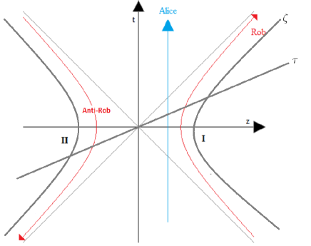
Figure 1: Minkowski spacetime and Rindler coordinate

We consider two modes of a Dirac field described by relatively accelerated parties; an inertial observer Alice (A) and a uniformly accelerated observer Rob (R) moving with a constant acceleration $a$. Each of the two parties is assumed to possess a detector sensitive only to one of the two modes. We focus on the Unruh effect for Dirac particles as experienced by Rob [92]. When a given Dirac mode is in the vacuum state from an inertial perspective, Rob’s detector perceives a Fermi-Dirac distribution of particles. Alice moves in the Minkowski plane with the coordinates $(t,z)$, as shown in Fig. (1). The Minkowski coordinates are the most suitable to describe the field from an inertial perspective. However, a uniformly accelerated observer is unable to access information about the whole of spacetime, because a communication horizon appears from his perspective. Hence, for formulating this phenomenon, the setting of the constant acceleration may be conveniently described by the Rindler coordinate $(\tau,\zeta)$ involving two disconnected regions I and II. In this coordinates, one can describe the uniformly accelerated Rob to travel on a hyperbola constrained to region I, as shown in Fig. (1). In fact, Rob has no access to the field modes in the causally disconnected region II. Hence, he must trace over the inaccessible region II, leading to an unavoidable loss of information about the state and essentially resulting in the detection of a mixed state. Under the single mode approximation, the Minkowski vacuum state $|0\rangle_{M}$ and the only excited state (one-particle state) $|1\rangle_{M}$ may be expressed in terms of the Rindler regions I and II states:

$$|0\rangle_{M}=\text{cos}~{}r|0\rangle_{I}|0\rangle_{II}+\text{sin}~{}r|1\rangle_{I}|1\rangle_{II},\\$$ (21)

$$|1\rangle_{M}=|1\rangle_{I}|0\rangle_{II}$$ (22)

where the dimensionless acceleration parameter $r$ is defined by $r=\text{arccos}\sqrt{1+e^{\frac{-2\pi\omega}{a}}}$ in which $\omega$ and $a$ are the Unruh mode frequency and acceleration, respectively, with $0<a<\infty$ and hence $r\in\left[0,\pi/4\right]$.

In order to investigate how the measurement before and after accelerating Rob, affects the process of parameter estimation, we consider the following scenario [93]:

(i) Initially, Alice and Rob share the entangled state

$$|\Psi\left(1\right)\rangle=\text{sin}\left(\frac{\vartheta}{2}\right)|0\rangle_{A}|0\rangle_{R}+\text{cos}\left(\frac{\vartheta}{2}\right)~{}\text{e}^{i\varphi}|1\rangle_{A}|1\rangle_{R};~{}~{}\ 0\leq\vartheta\leq\pi,\ 0\leq\varphi\leq 2\pi.$$ (23)

(ii) A PM is performed by Rob on his own particle before the acceleration (i.e., at time $\tau=0$).

(iii) We assume that Rob undergoes uniform acceleration $a$ and hence states $|0\rangle_{R}$ and $|1\rangle_{R}$ should be expanded as Eqs. (21) and (22), respectively.

(IV) After Rob’s acceleration, the operation of partial measurement reversal (PMR) is implemented by Rob in the region I.

Assuming that the measurements have been performed successfully, we obtain the following mixed state between Alice and Rob after tracing over region II:

$$\rho_{A,R}=\frac{1}{N}\left(\begin{array}[]{cccc}\text{sin}^{2}\frac{\vartheta}{2}~{}\overline{p}~{}\text{cos}^{2}r&0&0&\text{sin}~{}\frac{\vartheta}{2}\text{cos}~{}\frac{\vartheta}{2}~{}e^{-i\varphi}~{}\sqrt{\overline{pq}}~{}\text{cos}r\\ 0&\text{sin}^{2}\frac{\vartheta}{2}~{}\overline{pq}~{}\text{sin}^{2}r&0&0\\ 0&0&0&0\\ \text{sin}~{}\frac{\vartheta}{2}\text{cos}~{}\frac{\vartheta}{2}~{}e^{i\varphi}~{}\sqrt{\overline{pq}}~{}\text{cos}r&0&0&\text{cos}^{2}\frac{\vartheta}{2}~{}\overline{q}\\ \end{array}\right),~{}~{}~{}$$ (28)

where $N=\text{sin}^{2}\frac{\vartheta}{2}~{}\overline{p}~{}\text{cos}^{2}r+\text{sin}^{2}\frac{\vartheta}{2}~{}\overline{pq}~{}\text{sin}^{2}r+\text{cos}^{2}\frac{\vartheta}{2}~{}\overline{q}$ is the normalization factor and $\overline{p}=1-p$ as well as $\overline{q}=1-q$.

4 Premeasurement and postmeasurement effects on the behaviour of QFI

4.1 Weight parameter estimation

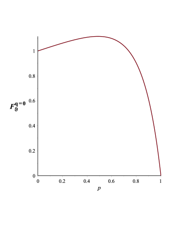
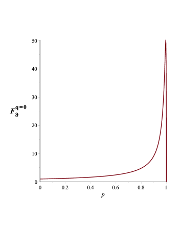
Figure 2: The QFI corresponding to the estimation of weight parameter for (a) $\vartheta=1.9$ and (b) $\vartheta=3$ when no post-measurement is performed.

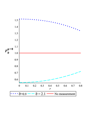
Figure 3: The QFI corresponding to the estimation of weight parameter for $q=0.6$ and different values of $\vartheta$ when only the postmeasurement is made.

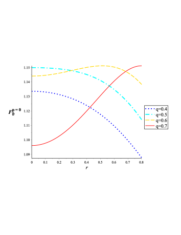
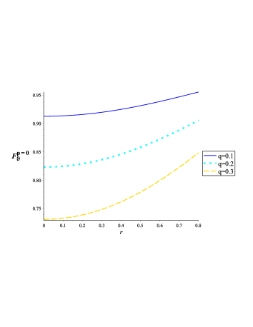
Figure 4: The QFI corresponding to the estimation of weight parameter for (a) $\vartheta=1.2$ as well as (b) $\vartheta=2.6$ and different values of $q$ when only the postmeasurement is made.

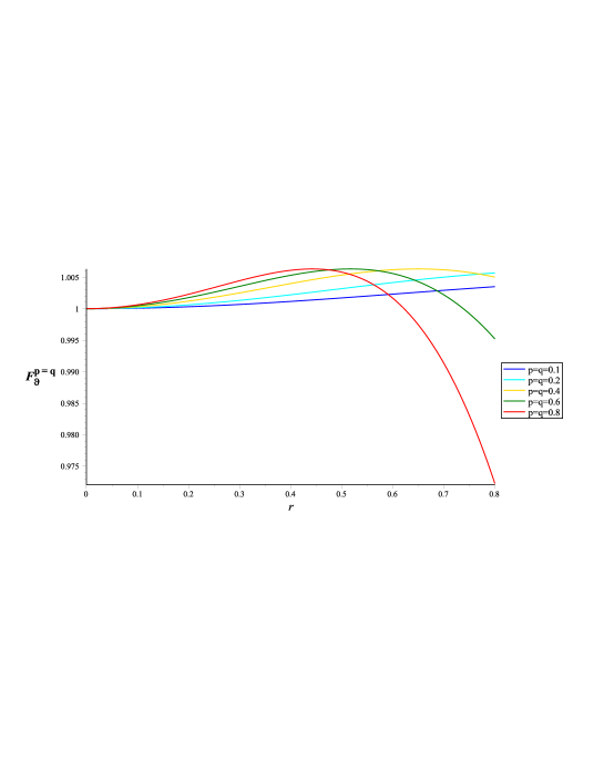
Figure 5: The QFI versus $r$ for $\vartheta>\pi/2~{}(\vartheta=1.65)$ when both measurements are made with equal strength.

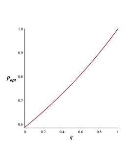
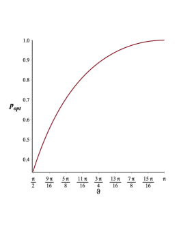
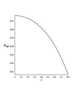
Figure 6: The optimal value of premeasurement strength as functions of $q$, $\vartheta$, and $r$ for (a) $\vartheta=2$ as well as $r=0.5$; (b) $q=0.4$ as well as $r=0.5$, and (c) $q=0.7$ as well as $\vartheta=0.2$

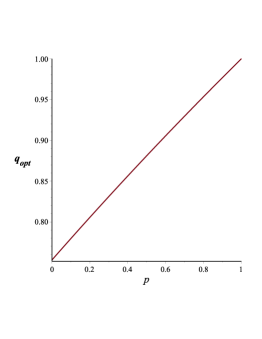
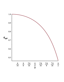
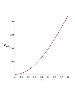
Figure 7: The optimal value of postmeasurement strength as functions of $p$, $\vartheta$, and $r$ for (a) $\vartheta=1$ as well as $r=0.5$; (b) $p=0.4$ as well as $r=0.5$, and (c) $p=0.7$ as well as $\vartheta=1$

In this section, we focus on the estimation of the weight parameter $\vartheta$. For calculation of the QFI, we use the following method [13]. First, the block diagonal state (28) should be written in the form $\rho_{A,I}=\bigoplus^{n}_{i=1}\rho_{i}$, in which $\bigoplus$ represents the direct sum. Then, it can be checked that the SLD operator may be written as $L=\bigoplus^{n}_{i=1}L_{i}$, where $L_{i}$ indicates the corresponding SLD operator for $\rho_{i}$. It can be shown that the SLD operator for the $i$th block is given by [88]

$$L_{i}=\frac{1}{\mu_{i}}\left[\partial_{x}\rho_{i}+\xi_{i}\rho^{-1}_{i}-\partial_{x}\mu_{i}\right],$$ (29)

where $\xi_{i}=2\mu_{i}\partial_{x}\mu_{i}-\partial_{x}P_{i}/4$ in which $\mu_{i}=\text{Tr}\rho_{i}/2$ and $P_{i}=\text{Tr}\rho^{2}_{i}$. Note that $\xi_{i}$ vanishes if det$\rho_{i}=0$.

Constructing SLD $L$ with this method and inserting it into Eq. (12) with density matrix (28), we obtain the following expression for the QFI associated with weight parameter $\vartheta$:

$$F_{\vartheta}=\,{\frac{-8~{}\overline{q}\overline{p}\left(-\overline{q}+\left(\overline{q}-1\right)\cos\left(2\,r\right)-1\right)}{\big{[}-\left(2\,\overline{q}-2\right)\overline{p}\cos\left(2\,r\right)\sin^{2}\left(\vartheta/2\right)+\overline{p}+\overline{qp}+2\,\overline{q}-\left(\overline{qp}+\overline{p}-2\,\overline{q}\right)\cos\left(\vartheta\right)\big{]}^{2}}}.$$ (30)

We find when $p,q\rightarrow 0$, then $F_{\vartheta}\rightarrow 1$. Therefore, when no measurement is performed, the Unruh decoherence and the initial state do not affect on the weight parameter estimation. Especially, when the post-measurement does not perform, i.e., $q=0$, the QFI is reduced to:

$$F^{q=0}_{\vartheta}={\frac{4-4\,p}{\left(\cos\left(\vartheta\right)p-p+2\right)^{2}}},$$ (31)

denoting that the QFI is unaffected by the Unruh effect. Hence, the second measurement plays a key role for determining whether or not the estimation of the weight parameter is affected by the Unruh effect. Now investigating (31), it is observed that for $\vartheta<\pi/2$, the QFI degrades with increasing $p$, while for $\vartheta>\pi/2$, the QFI may increase with $p$ (see Fig. 2). Especially, as seen in Fig. 2, when $\vartheta\rightarrow\pi$, the estimation of the weight parameter is enhanced considerably with increase in the pre-measurement strength, unless $p\rightarrow 1$, in that case the QFI decreases with a steep slope. Therefore, the PM may guarantees enhancement of the weight parameter estimation, however approaching the sharp von Neumann measurement sleeply decreases the precision of the estimation. In order to obtain the optimum value of the PM strength for the best estimation, in the absence of the postmeasurement, we derive (31) in terms of $p$. The result is as follows:

$$p_{q=0}^{\text{opt}}={\frac{2\cos\left(\vartheta\right)}{\cos\left(\vartheta\right)-1}},$$ (32)

leading to the optimal QFI

$$(F^{q=0}_{\vartheta})_{\text{opt}}=\dfrac{1}{\text{sin}^{2}\vartheta}.$$ (33)

Figure 4 illustrates the pure effects of the post-measurement on the QFI and it is compared with the case that no measurement is performed. The second PM, as described above, plays the role of a quantum key for manifestation of the Unruh effect. When only the second measurement is performed, i.e., $p=0$, we see if $\vartheta<\pi/2$, the accuracy of the parameter estimation is improved compared to the situation in which no measurement has been made $(F_{\vartheta}=1)$, but when $\vartheta>\pi/2$, it is not possible to achieve a better estimation. Moreover, similar to the previous discussion, approaching the complete von Neumann measurement, $q\rightarrow 1$, causes the precision of the estimation to diminish and be less than unity.

In Fig. 4, we analyse how the postmeasurement affects the QFI behaviour versus the Unruh effect in the absence of the premeasurement. As seen in Fig. 4(a), if $\vartheta<\pi/2$, for small values of $q$, the QFI decreases with growth of the acceleration parameter $r$. Nevertheless, with strengthening the postmeasurement, the precision of the estimation may be enhanced with increase in the acceleration and then it decreases. The optimal point is as follows:

$$r_{p=0}^{\text{opt}}=\frac{1}{2}\,\arccos\left({\frac{\left(4\,q-8\right)\sin^{2}\left(\vartheta/2\right)-q\cos\left(\vartheta\right)-3\,q+4}{2q\sin^{2}\left(\vartheta/2\right)}}\right).$$ (34)

Inserting it in Eq. (30) with $p=0$, we can obtain the following expression for the optimal QFI:

$$(F^{p=0}_{\vartheta})_{\text{opt}}=\dfrac{1}{\text{sin}^{2}\vartheta}.$$ (35)

Moreover, for large values of $q$, the QFI monotonously increases as the Unruh acceleration raises. Similarly, when $\vartheta>\pi/2$, as illustrated in Fig. 4(b), the QFI and hence the precision of estimation monotonously are enhanced with increase in the acceleration.

Now we focus on behaviour of the QFI when both measurements are made simultaneously. In the special case that $\vartheta>\pi/2$ and $p=q$ the QFI may increase compared it to the situation that no measurement is performed (i.e., it is possible to obtain an optimal value or an enhanced value for the QFI such that $F^{p=q}_{\vartheta}>1$ ). Figure 5 shows the QFI as a function of the Unruh acceleration parameter for $p=q$. Generally, the maximum point of the plot of QFI versus $r$ is given by:

$$r_{\text{opt}}=\frac{1}{2}\,\arccos\left({\frac{\left(\left(q-2\right)p-3\,q+4\right)\cos^{2}\left(\vartheta/2\right)-\left(q-2\right)\left(-1+p\right)}{q\left(1-p\right)\sin^{2}\left(\vartheta/2\right)}}\right),$$ (36)

provided that it exists. Hence, the following compact expression for the optimal value of the QFI associated with the weight parameter is obtained:

$$(F_{\vartheta})_{\text{opt}}=\dfrac{1}{\text{sin}^{2}\vartheta},$$ (37)

which is clearly independent of $p$ and $q$. Therefore, although performing the measurements may vary the acceleration at which the optimal estimation occurs, the optimal value of the QFI, is completely unaffected by the strength of the measurements. Moreover, Eq. (36) gives us a proper criterion for existence of the QFI optimal value. If the substituted parameters lead to unphysical values for the acceleration parameter $r$, we conclude that no optimal value is achievable for the QFI in terms of $r$. Under this situation, i.e., absence of any optimal value for the QFI, we find that if both measurements are performed simultaneously with equal strength (p=q), the QFI is always lower bounded via $F^{p=q}_{\vartheta}>1$, showing enhancement of estimation compared to the case that no measurements are carried out

In the context of applying both measurements, we generally consider two important regimes, i.e., $\vartheta>\pi/2$ and $\vartheta<\pi/2$ for investigating the optimal behaviour of the QFI in terms of $p$ or $q$ when other parameters are constant. Solving equations $\dfrac{\partial F_{\vartheta}}{\partial p}=0$ and $\dfrac{\partial F_{\vartheta}}{\partial q}=0$, we can obtain the following expressions for $p_{opt}$ and $q_{opt}$, respectively:

$$p_{opt}={\frac{q\cos\left(2\,r\right)+2\,\left(q-1\right)\csc^{2}\left(\vartheta/2\right)-3\,q+4}{q\cos\left(2\,r\right)-q+2}}~{}~{}~{}~{}~{}~{}~{}~{}~{}~{}~{}~{}~{}~{}~{}~{}\vartheta>\pi/2,$$ (38)

$$q_{opt}={\frac{2\,\left(p-2\right)\cos\left(\vartheta\right)-2\,p}{2\,\left(p-1\right)\cos\left(2\,r\right)\sin^{2}\left(\vartheta/2\right)+\left(p-3\right)\cos\left(\vartheta\right)-p-1}}~{}~{}~{}~{}\vartheta<\pi/2,$$ (39)

denoting when $\vartheta>\pi/2~{}(\vartheta<\pi/2)$, the QFI reveals optimal behaviour in terms of $p~{}(q)$. Figures 6 and 8 illustrate how these optimal points vary in terms of other parameters. Especially, Fig. 6 shows strengthening the postmeasurement, we should increase the strength of the premeasurement for achieving the optimal value of the QFI. Moreover, as seen in Fig. 6, larger values of $\vartheta$ (the parameter that should be estimated), need larger values of $p$ for obtaining the optimal value. On the other hand, Fig. 6 shows that more weak premeasurements are required for attaining the optimal QFI when the accelerated observer moves with more larger acceleration. Finally, Fig. 8 illustrates the behaviour of $q_{opt}$ as functions of $p$, $\vartheta$ and $r$. As plotted in Fig. 7, strengthening the premeasurement requires increase of the postmeasurement strength for achieving the optimal value of the QFI. Besides, contrary to the previous case, smaller values of $\vartheta$ need more strong postmeasurements for achieving the optimal estimation (see Fig. 7). Moreover, when the accelerated observer moves with more larger acceleration, we should strengthen the postmeasurement for attaining the optimal QFI (see Fig. 7).

It should be noted that substituting $p_{opt}$ ($q_{opt}$) with $p$ ($q$) in Eq. (30), we obtain the optimal value similar to one given in Eq. (37). Therefore, in both regimes, i.e., $\vartheta>\pi/2$ and $\vartheta<\pi/2$, achieving the optimal value, we can improve the parameter estimation compared to the scenario in which no measurements are carried out.

4.2 Phase parameter estimation

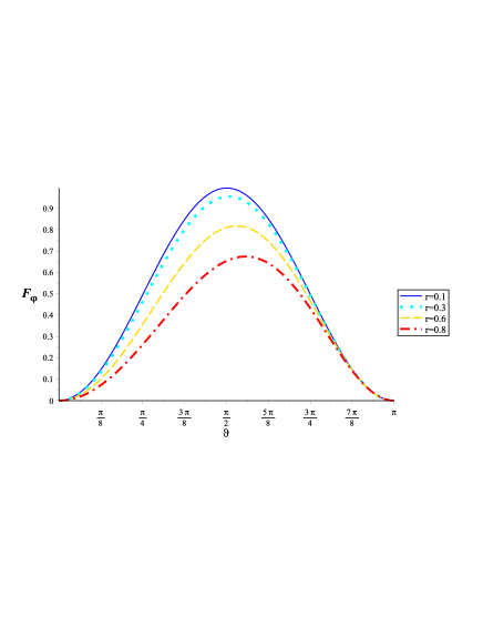
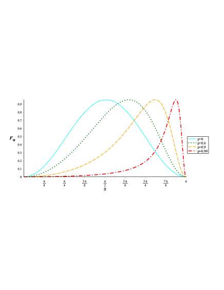
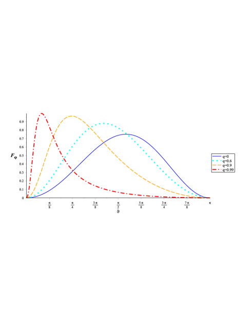
Figure 8: The QFI associated with the phase parameter as a function of $\vartheta$; (a) The QFI for $p=q=0$ and different values of $r$. (b) The same quantity for $r=0.2,~{}q=0$, and different values of $p$. (c) The same quantity for $r=0.7,~{}p=0$, and different values of $q$

Estimating phase parameter $\varphi$ leads to the following expression for the corresponding QFI:

$$F_{\varphi}={\frac{-2~{}\overline{pq}\cos^{2}\left(r\right)\bigg{(}\cos\left(2\,r\right)\left(\cos\left(\vartheta\right)-1\right)\overline{p}-\overline{p}-2\,\overline{q}+\left(\overline{p}-2\,\overline{q}\right)\cos\left(\vartheta\right)\bigg{)}\tan^{2}\left(\vartheta/2\right)}{\bigg{(}2\,\overline{p}\cos^{2}\left(r\right)\sin^{2}\left(\vartheta/2\right)+2\,\overline{pq}\sin^{2}\left(r\right)\sin^{2}\left(\vartheta/2\right)+\overline{q}+\overline{q}\cos\left(\vartheta\right)\bigg{)}\big{(}\overline{p}\cos^{2}\left(r\right)\tan^{2}\left(\vartheta/2\right)+\overline{q}\big{)}^{2}}}$$ (40)

In order to discuss the optimal behaviour of the QFI, it is assumed that we have no control over the initial state. First, the QFI variation versus the acceleration parameter when no measurements are made is investigated (see Fig. 8). It is observed, in the absence of any measurement, when the accelerated observer moves with larger acceleration, the optimal value of the QFI decreases and occurs for a larger value of the initial parameter $\vartheta$.

Because there is no control over $\vartheta$, we intend to match the optimal $\vartheta$ to the predetermined $\vartheta$. Figures 8 and Fig. 8 illustrates how this strategy may be implemented by controlling the strength of the measurements. Figure 8 shows that increase of the premeasurement strength shifts the optimal point to the right and the same time it does not considerably change the optimal value of the QFI. On the other hand, from Fig. 8, we find that increase of the postmeasurement strength shifts the optimal point to the left and interestingly raises the optimal value of the QFI, leading to enhancement of the phase parameter estimation compared to the case that no measurements are carried out. Overall, using weak measurements, we can control the optimal point at which the QFI is maximized, such that it coincides with the initial value defined in Eq. (23).

4.2.1 Lower bound on QFI with LQU

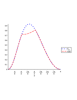
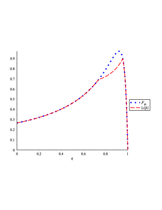
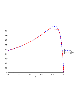
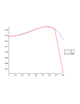
Figure 9: Comparison between QFI associated with the phase parameter and LQU. (a) Both quantities as functions of $\vartheta$ for $p=0.4$, $r=0.7$, and $q=0.8$. (b) The same quantities as functions of $q$ for $p=0.4$, $r=0.7$, and $\vartheta=0.9$. (c) The same quantities as functions of $p$ for $q=0.2$, $r=0.1$, and $\vartheta=2.3$. (d)The same quantities as functions of $r$ for $q=0.5$, $p=0$, and $\vartheta=1.8$.

The analytical expression for LQU of quantum state (28) is given in Appendix B. We first briefly review an important discussion from [60]. Given a (generally mixed) bipartite state $\rho$ used as a probe, subsystem A experiences a unitary transformation so that the bipartite state transforms into $\rho_{\varphi}=U_{\varphi}\rho U^{\dagger}_{\varphi}$, where $U_{\varphi}=\text{exp}^{-i\varphi H_{A}}$, with $H_{A}$ a local Hamiltonian on A, which we assume to have a nondegenerate spectrum. The initial state (23) may be prepared by the above scenario. Under this condition, it has been shown that the QFI associated with the phase shift majorizes the skew information of the Hamiltonian and therefore the LQU [60, 94], i.e., $\mathcal{U}_{A}(\rho)\leq I(\rho,H_{A})=I(\rho_{\varphi},H_{A})\leq\frac{1}{4}F_{\varphi}$. It should be noted that in this model, the other steps of the estimation process are assumed to be noiseless. Besides, in [63], it has been shown that for a model, consisting of two qubits interacting with independent non-Markovian environments, when we consider the effects of the environment and the coupling interaction between subsystems, the QFI and LQU do not satisfy the similar relationship generally. Now we investigate whether or not this bound holds for our model including the PMs and the Unruh effect.

Here, our numerical computation shows that the QFI associated with the phase parameter is bounded from below by the LQU which is the measure of amount of quantum correlations in the mixed state (28) used for parameter estimation (see Fig. 9), i.e.,

$$\mathcal{U}_{A}(\rho_{A,I})\leq F_{\varphi}.$$ (41)

Especially, if the QFI reveals no optimal behaviour as a function of one of the parameters shown in Figs. 9-9 for determined values of other parameters, equality $F_{\varphi}=\mathcal{U}_{A}(\rho_{A,I})$ holds. Moreover, inequality (41) refers to the fact that the quantum correlations measured by LQU, are a sufficient resource to ensure that some information about the phase parameter can be extracted from the system in the process of estimation. In addition, for probe quantum states with any nonzero amount of discord, and for $M\gg 1$ repetitions of the estimation process, the optimal detection strategy, asymptotically saturating the quantum Cramér-Rao bound, leads to production of an estimator $\tilde{\varphi}_{best}$ with the following necessarily limited variance:

$$Var(\tilde{\varphi}_{best})=\dfrac{1}{MF_{\varphi}}\leq\dfrac{1}{M\mathcal{U}_{A}(\rho_{A,I})}$$ (42)

Therefore, we find that, in the relativistic framework, the quantum correlations measured by the LQU, are a sufficient resource to guarantee an upper bound on the smallest possible variance with which the phase parameter can be measured in the presence of PMs and Unruh effect.

4.2.2 Upper bound on QFI with MSC

Using Eq. (48) and density matrix (28), we obtain the following expression for MSC

$$\Lambda(\rho_{A,I})={\frac{1}{\sqrt{q+\left(1-q\right)\sec^{2}\left(r\right)}}}$$ (43)

where it is completely unaffected by the premeasurement and initial preparation of the system. Moreover, although the acceleration degrades the MSC, strengthening the postmeasurement can improve it (see Fig. 10). In particular, when $q\rightarrow 1$, the MSC becomes robust against the Unruh effect.

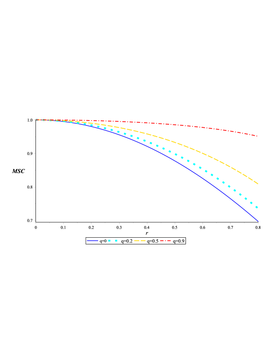
Figure 10: MSC versus $r$ for different values of $q$.

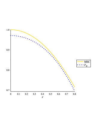
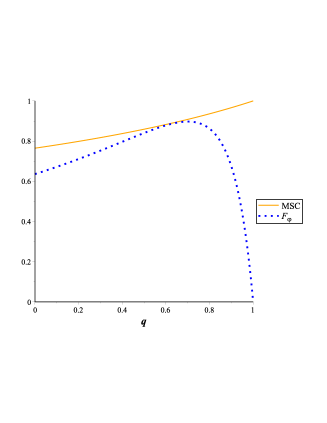
Figure 11: MSC as an upper bound on the QFI (a) Both quantities as functions of $r$ for $p=0.2$, $\vartheta=1.8$, and $q=0.1$. (b) The same quantities as functions of $q$ for $p=0.2$, $r=0.7$, and $\vartheta=1.8$.

Generally, the exact computation of the QFI is difficult because it usually needs diagonalization of the density matrix. Hence, resorting to upper bounds on the QFI may be beneficial both theoretically and practically [97, 98]. Now, we reveal an important relationship between the QFI associated with the phase parameter and the MSC. As seen in Fig. 11, the MSC determines an upper bound on the QFI associated with the phase parameter. In particular, this upper bound is approximately saturated near optimal point $q_{opt}$ at which the QFI is maximized (see Fig. 11).

5 Summary and conclusions

To summarize, we have completely discussed the optimal behaviour of the QFI for two modes of a Dirac field detected by an inertial observer Alice and a uniformly accelerated observer Rob, experiencing the Unruh effect. In particular, we have investigated the effects of weak measurements, performed before and after accelerating Rob, on the optimal estimation of the weight and phase parameters of the initial state of the system. It was found that the weak measurements may partially compensate the decreasing effects of the Unruh decoherence on the accuracy of the parameter estimation. This enhancement of estimation could be attributed to the probabilistic nature of weak measurements, because in the case of projective measurement ($p$ or $q$=1), the QFI jumps to zero and no information can be extracted from the process of quantum estimation. On the other hand, estimating weight parameter $\vartheta$, we obtain the QFI trapping with value $F^{p=q=0}_{\vartheta}=1$ in the absence of PMs.

In the case of estimating weight parameter $\vartheta$, it was interestingly demonstrated that the second PM operates as a quantum key for manifestation of the Unruh effect such that when $q=0$, the QFI is unaffected by the Unruh decoherence. Under this situation, the first PM may guarantees the enhancement of the estimation provided that $\vartheta>\pi/2$. Besides, we illustrated that it is possible to design the PMs such that the optimal estimation is realized. It was found that achieving the optimal value of the QFI, we can improve the parameter estimation compared to the scenario in which no measurements are carried out. Moreover, we found that if both measurements are performed simultaneously with equal strength $(p=q)$, the estimation is enhanced compared to the case that no measurements are performed. In the case of optimizing the phase estimation, nevertheless we have no control over the initial state, it was shown that the weak measurements may be used to match the optimal $\vartheta$ to its predetermined value.

Besides, it was found that the QFI associated with the phase parameter is bounded from below by the LQU. More interestingly, our numerical calculation revealed that the MSC can be utilized to obtain an upper bound, approximately saturable, on the QFI in our relativistic scenario. We also obtained a compact formula for the MSC of X-states.

Finally, It is worth noting that the PM may be easily applied to different types of qubits such as spin qubits, optical polarization qubits, and Josephson junction qubits, etc. The experimental implementation of PM has been realized in a photonic architecture [99, 100], and Josephson junction [101]. Alternatively, the PMs could be described with projective measurements in a larger Hilbert space including an ancilla qubit [102]. Therefore, the performance of the PM on the target qubit is equivalent to the action of von Neumann projective measurement on the ancilla qubit previously coupled to it. Hence, our scheme can be realized by current technology for different types of qubits.

Appendix A Analytical expression of MSC for X-states

The density matrix of a two-qubit X state [95] shared by Alice and Rob takes the following form in the computational basis $\{|00\rangle,|01\rangle,|10\rangle,|11\rangle\}$

$$\rho_{X}=\left(\begin{array}[]{cccc}\rho_{11}&0&0&\rho_{14}\\ 0&\rho_{22}&\rho_{23}&0\\ 0&\rho_{32}&\rho_{33}&0\\ \rho_{41}&0&0&\rho_{44}\\ \end{array}\right)$$ (44)

where $\rho_{23}=\rho_{32}^{*}$, $\rho_{14}=\rho_{41}^{*}$, and $\sum\limits_{i=1}^{4}\rho_{ii}=1$. Using (7), we find the Rob’s steering ellipsoid is centered at

$$\textbf{C}_{X}=\left(\begin{array}[]{ccc}0\\ 0\\ {\frac{\rho_{{11}}\rho_{{33}}-\rho_{{22}}\rho_{{44}}}{\left(\rho_{{11}}+\rho_{{22}}\right)\left(\rho_{{33}}+\rho_{{44}}\right)}}\\ \end{array}\right).$$ (45)

Moreover, Eq. (8) leads to the matrix

$$Q_{X}=\left(\begin{array}[]{ccc}Q_{11}&Q_{12}&0\\ Q_{21}&Q_{22}&0\\ 0&0&Q_{33}\\ \end{array}\right)$$ (46)

where

$$Q_{11}={\frac{\left|\rho_{{14}}+\rho_{{23}}\right|^{2}}{\left(\rho_{{11}}+\rho_{{22}}\right)\left(\rho_{{33}}+\rho_{{44}}\right)}}$$

$$Q_{12}=Q_{21}={\frac{-2~{}\text{Im}\left(\rho_{{14}}\rho_{{32}}\right)}{\left(\rho_{{11}}+\rho_{{22}}\right)\left(\rho_{{33}}+\rho_{{44}}\right)}}$$

$$Q_{22}={\frac{\left|\rho_{{14}}-\rho_{{23}}\right|^{2}}{\left(\rho_{{11}}+\rho_{{22}}\right)\left(\rho_{{33}}+\rho_{{44}}\right)}}$$ (47)

$$Q_{33}={\frac{\bigg{(}\left(\rho_{{11}}-\rho_{{44}}\right)^{2}-\left(\rho_{{22}}-\rho_{{33}}\right)^{2}+1-2\,(\rho_{11}+\rho_{44})\bigg{)}^{2}}{\bigg{(}4~{}\left(\rho_{{11}}+\rho_{{22}}\right)\left(\rho_{{33}}+\rho_{{44}}\right)\bigg{)}^{2}}}$$

The eigenvalues of matrix $Q$ are the squares of the ellipsoid semiaxes and its eigenvectors give the orientation of these axes [96]. Because of block form of $Q_{X}$, one of its semiaxes is oriented parallel to b. In detail, when $\rho$ is an X-state, the Bloch vector b lies along an axis of the Rob’s steering ellipsoid, and $\Lambda$ is the length of the longest of the other two semiaxes [67]. Following this point, we find that the analytical expression of MSC for X-states is given by

$$\Lambda(\rho_{X})={\frac{\left|\rho_{23}\right|+\left|\rho_{14}\right|}{\sqrt{\left(\rho_{{11}}+\rho_{{22}}\right)\left(\rho_{33}+\rho_{44}\right)}}}$$ (48)

Appendix B Expression for LQU

After tedious calculation, one can obtain the LQU for quantum state (28):

$$\mathcal{U}_{A}=1-\text{max}(W_{1},W_{2}),$$ (49)

where $W_{1}$ and $W_{2}$ are expressed as

$$W_{1}=\frac{\sin\left(r\right)\sin\left(\vartheta/2\right)\sqrt{\overline{p}{\overline{q}}^{3}\bigg{(}-\cos\left(\vartheta\right)\big{(}\overline{p}\cos\left(2\,r\right)+\overline{p}-2\,\overline{q}\big{)}+\overline{p}\cos\left(2\,r\right)+\overline{p}+2\,\overline{q}\bigg{)}}}{{\it N}\,\left(\overline{p}\cos^{2}\left(r\right)\tan^{2}\left(\vartheta/2\right)+\overline{q}\right)}$$ (50)

and

$$W_{2}=\dfrac{l_{1}+l_{2}+l_{3}}{{4N}\,\left(\overline{p}\cos^{2}\left(r\right)\tan^{2}\left(\vartheta/2\right)+\overline{q}\right)^{2}}$$ (51)

in which $l_{i}$’s are given by

$$l_{1}={\overline{q}}^{2}\left(\overline{p}+2\,\overline{q}\right)-\overline{p}\cos\left(2\,r\right)\left(\cos\left(\vartheta\right)-1\right)\bigg{(}\overline{q}-\overline{p}\cos^{2}\left(r\right)\tan^{2}\left(\vartheta/2\right)\bigg{)}^{2},\\$$

$$l_{2}=-\left(\overline{p}-2\,\overline{q}\right)\cos\left(\vartheta\right)\bigg{(}\overline{q}-\overline{p}\cos^{2}\left(r\right)\tan^{2}\left(\vartheta/2\right)\bigg{)}^{2}+\overline{p}\left(\overline{p}+2\,\overline{q}\right)\cos^{2}\left(r\right)\tan^{2}\left(\vartheta/2\right)\left(\overline{p}\cos^{2}\left(r\right)\tan^{2}\big{(}\vartheta/2\big{)}-2\,\overline{q}\right),\\$$

$$l_{3}=4\,\overline{p}\overline{q}\sin^{2}\left(r\right)\sin^{2}\left(\vartheta/2\right)\bigg{(}\overline{p}\cos^{2}\left(r\right)\tan^{2}\left(\vartheta/2\right)+\overline{q}\bigg{)}^{2}.\\$$

References

- [1] C. W. Helstrom, Quantum Detection and Estimation Theory (Academic, New York, 1976).
- [2] M.G.A. Paris, Int. J. Quant. Inf. 7, 125 (2009).
- [3] X. M. Lu, X. Wang, and C. P. Sun, Phys. Rev. A 82, 042103 (2010).
- [4] L. Chang, N. Li, S. Luo, and H. Song, Phys. Rev. A 89, 042110 (2014).
- [5] Z. Jiang, Phys. Rev. A 89, 032128 (2014).
- [6] W. Zhong, Z. Sun, J. Ma, X. Wang, and F. Nori, Phys. Rev. A 87, 022337 (2013).
- [7] J. Ma and X. G. Wang, Phys. Rev. A 80, 012318 (2009).
- [8] Z. Sun, J. Ma, X. M. Lu, and X. G. Wang, Phys. Rev. A 82, 022306 (2010).
- [9] Y. Yao, X. Xiao, L. Ge, X. G. Wang, and C. P. Sun, Phys. Rev. A 89, 042336 (2014).
- [10] V. Giovannetti, S. Lloyd, and L. Maccone, Phys. Rev. Lett. 96, 010401 (2006).
- [11] H. Rangani Jahromi, M. Amniat-Talab, Ann. Phys. 355, 299 (2015).
- [12] J. Ma, Y. x. Huang, X. Wang, and C. P. Sun, Phys. Rev. A 84, 022302 (2011).
- [13] H. Rangani Jahromi, Opt. Commun. 411, 119 (2018).
- [14] H. Rangani Jahromi and M. Amniat-Talab, Ann. Phys. 360, 446461 (2015).
- [15] V. Giovannetti, S. Lloyd, and L. Maccone, Nat. Photon. 5, 222 (2011).
- [16] Y. Israel, S. Rosen, and Y. Silberberg, Phys. Rev. Lett. 112, 103604 (2014).
- [17] G. Y. Xiang, B. L. Higgins, D. W. Berry, H. M. Wiseman, and G. J. Pryde, Nat. Photon. 5, 43 (2011).
- [18] M. Schleier-Smith, M., H. I. D. Leroux, and V. Vuletić, Phys. Rev. Lett. 104, 073604 (2010).
- [19] A. Sørensen, L. M. Duan, J. I. Cirac, and P. Zoller, Nature 409, 63 (2001).
- [20] R. Joza, D.S. Abrams, J.P. Dowling, C.P. Williams, Phys. Rev. Lett. 85, 2010 (2000).
- [21] J.J. Bollinger, W.M. Itano, D.J. Wineland, and D.J. Heinzen, Phys. Rev. A 54, R4649 (1996).
- [22] A. Peters, K.Y. Chung, and S. chu, Nature (London) 400, 849 (1999).
- [23] I. Fuentes-Schuller and R. B. Mann, Phys. Rev. Lett. 95, 120404 (2005)
- [24] G. Adesso, I. Fuentes-Schuller, and M. Ericsson, Phys. Rev. A 76, 062112 (2007).
- [25] J. León and E. Martín-Martínez, Phys. Rev. A 80, 012314 (2009).
- [26] G. Adesso and I. Fuentes-Schuller, Quantum Inf. Comput. 9, 0657 (2009).
- [27] E. Martín-Martínez, L. J. Garay, and J. León, Phys. Rev. D 82, 064006 (2010).
- [28] E. Martín-Martínez and J. León, Phys. Rev. A 80, 042318 (2009).
- [29] E. Martín-Martínez and J. León, Phys. Rev. A 81, 032320 (2010).
- [30] I. Fuentes, R. B. Mann, E. Martín-Martínez, and S. Moradi, Phys. Rev. D 82, 045030 (2010).
- [31] E. Martín-Martínez, L. J. Garay, and J. León, Phys. Rev. D 82, 064028 (2010).
- [32] E. Martín-Martínez and J. León, Phys. Rev. A 81, 052305 (2010).
- [33] E. Martín-Martínez, ”Relativistic Quantum Information:developments in Quantum Information in general relativistic scenarios,” PhD Thesis, Complutense Universityof Madrid (2011) [arXiv:1106.0280 [quant-ph].
- [34] D. E. Bruschi, J. Louko, E. Martín-Martínez, A. Dragan, and I. Fuentes, Phys. Rev. A 82, 042332 (2010).
- [35] P. M. Alsing and I. Fuentes, Classical Quantum Gravity 29, 224001 (2012).
- [36] E. Martín-Martínez, D. Aasen, and A. Kempf, Phys. Rev. Lett. 110, 160501 (2013)
- [37] A. R. Lee and I. Fuentes, Phys. Rev. D 89, 085041 (2014).
- [38] M. Lanzagorta, Quantum Information in Gravitational Fields (Institute of Physics Publishing, Bristol, 2014)
- [39] N. Friis and I. Fuentes, J. Mod. Opt. 60, 22 (2013).
- [40] M. Aspachs, G. Adesso, and I. Fuentes, Phys. Rev. Lett. 105, 151301 (2010).
- [41] T. G. Downes, G. J. Milburn, and C. M. Caves, arXiv: 1108.5220.
- [42] D. Hosler, and P. Kok, Phys. Rev. A 88, 052112 (2013).
- [43] M. Ahmadi, D. E. Bruschi, N. Friis, C. Sabín, G. Adesso, and I. Fuentes, Sci. Rep. 4, 4996 (2014).
- [44] M. Ahmadi, D. E. Bruschi, and I. Fuentes, Phys. Rev. D 89, 065028 (2014).
- [45] Y. Yao, X. Xiao, L. Ge, X. G. Wang, and C. P. Sun, Phys. Rev. A 89, 042336 (2014).
- [46] J. C. Wang, Z. H. Tian, J. L. Jing, and H. Fan, Sci. Rep. 4, 7195 (2014).
- [47] C. Sabín, D. E. Bruschi, M. Ahmadi, and I. Fuentes, New J. Phys. 16, 085003 (2014).
- [48] J. Doukas, L. Westwood, D. Faccio, A. D. Falco, and I. Fuentes, Phys. Rev. D 90, 024022 (2014).
- [49] D. E. Bruschi, A. Datta, R. Ursin, T. C. Ralph, and I. Fuentes, Phys. Rev. D 90, 124001 (2014).
- [50] D. Ŝafránek, M. Ahmadi, and I. Fuentes, New J. Phys. 17, 033012 (2015).
- [51] S. P. Kish and T. C. Ralph, Phys. Rev. D 93, 105013 (2016).
- [52] C. Y. Huang, W. Ma, D. Wang, and L. Ye, Sci. Rep. 7, 38456 (2017).
- [53] X. Huang, J. Feng, Y. Zhang, H. Fan, Ann. Phys. 397, 336 (2018).
- [54] M. Jafarzadeh, H. Rangani Jahromi, and M. Amniat-Talab, Quantum Inf. Process 17, 165 (2018).
- [55] J. Kohlrus, D. E. Bruschi, and I. Fuentes, Phys. Rev. A 99, 032350 (2019).
- [56] Y. S. Kim, J. C. Lee, O. Kwon, and Y. H. Kim, Nat. Phys. 8, 117 (2012).
- [57] Y. Chen, J. Zou, Z.W. Long, and B. Shao, Sci. Rep. 7, 6160 (2017).
- [58] Z. Liu, L. Qiu, and F. Pan, Quantum Inf. Process. 16, 109 (2017).
- [59] K. Modi, A. Brodutch, H. Cable, T. Paterek, and V. Vedral, Rev. Mod. Phys. 84, 1655 (2012).
- [60] D. Girolami, T. Tufarelli, and G. Adesso, Phys. Rev. Lett. 110, 240402 (2013).
- [61] F.F. Fanchini, D.O. Soares Pinto, G. Adesso (eds.), Lectures on General Quantum Correlations and their Applications (Springer, 2017).
- [62] C. S. Yu, S. X. Wu, X. Wang, X. X. Yi and H. S. Song, Europhys. Lett. 107, 10007 (2014).
- [63] S.X. Wu, Y. Zhang, C.S. Yu, Ann. Physics (2018); DOI link: https://doi.org/10.1016/j.aop.2018.01.004.
- [64] S. D. Bartlett, T. Rudolph, and R. W. Spekkens, Rev. Mod. Phys. 79, 555 (2007).
- [65] V. Narasimhachar and G. Gour, Nat. Commun. 6, 7689 (2015).
- [66] S. Lloyd, J. Phys. Conf. Ser. 302, 012037 (2011)
- [67] X. Hu, A. Milne, B. Zhang, and H. Fan, Sci. Rep. 6, 19365 (2016).
- [68] B. Farajollahi, M. Jafarzadeh, H. Rangani Jahromi, and M. Amniat-Talab, Quant. Inf. Proc. 17, 119 (2018).
- [69] R. Demkowicz-Dobrzański, L. Maccone, Phys. Rev. Lett. 113, 250801 (2014).
- [70] H. Rangani Jahromi, J. Mod. Opt. 64, 1377 (2017).
- [71] A. N. Korotkov and A. N. Jordan, Phys. Rev. Lett. 97, 166805 (2006).
- [72] Q. Q. Sun, M. Al-Amri, and M. S. Zubairy, Phys. Rev. A 80, 033838 (2009).
- [73] Z. X. Man, Y. J. Xia, and N. B. An, Phys. Rev. A 86, 012325 (2012).
- [74] X. Xiao and Y. L. Li, Eur. Phys. J. D 67, 204 (2013).
- [75] N. Katz, M. Neeley, M. Ansmann, R. C. Bialczak, M. Hofheinz, E. Lucero, A. Oconnell, H. Wang, A. N. Cleland, J. M. Martinis, and A. N. Korotkov, Phys. Rev. Lett. 101, 200401 (2008).
- [76] Y. S. Kim, Y. W. Cho, Y. S. Ra, and Y. H. Kim, Opt. Express 17, 11978 (2009)
- [77] X. Xiao, Y. Yao, W.-J.Zhong, Y.-Ling and Y.-Mao Xie, Phys. Rev. A 93, 012307 (2016).
- [78] Z. Liu, L. Qiu, and F. Pan, Quantum Inf. Process. 16, 109 (2017).
- [79] Y Chen, J Zou, Z Long, B Shao, Sci. Rep. 7, 6160 (2017).
- [80] D. M. T. Benincasa, L. Borsten, M. Buck, and F. Dowker, Classical and Quantum Gravity 31, 075007 (2014).
- [81] S. Y. Lin, arXiv:1310.2504 (2013).
- [82] L. Seveso, M. A. C. Rossi, and M. G. A. Paris, Phys. Rev. A 95,012111 (2017).
- [83] P. Bogaert and D. Girolami, in Lectures on General Quantum Correlations and their Applications (Springer, 2017) pp. 159-179.
- [84] S. Jevtic, M. Pusey, D. Jennings, and T. Rudolph, Phys. Rev. Lett. 113, 020402 (2014).
- [85] S. Jevtic, M. J. W. Hall, M. R. Anderson, M. Zwierz, and H. M. Wiseman, J. Opt. Soc. Am. B 32, A40 (2015).
- [86] T. Baumgratz, M. Cramer, and M. B. Plenio, Phys. Rev. Lett. 113, 140401 (2014).
- [87] S. L. Braunstein and C. M. Caves, Phys. Rev. Lett. 72, 3439 (1994).
- [88] J. Liu, J. Chen, X. X. Jing, and X. Wang, J. Phys. A 49, 275302 (2016).
- [89] J. Liu, X. Jing, and X. Wang, Phys. Rev. A 88, 042316 (2013).
- [90] L. Jing, J. Xiao-Xing, Z. Wei, and W. Xiao-Guang, Commun. Theor. Phys. 61, 45 (2014).
- [91] J. Liu, H.-N. Xiong, and X. Song, F.and Wang, Physica A 410, 167 (2014).
- [92] M. Alsing, I. Fuentes-Schuller, R. B. Mann, and T. E. Tessier, Phys. Rev. A 74, 032326 (2006).
- [93] X. Xiao, Y. M. Xie, Y. Yao, Y. L. Li, and J. Wang, Ann. Phys. 390, 83 (2018).
- [94] S. Luo, Proc. Am. Math. Soc. 132, 885 (2004).
- [95] P. C. Obando, F. M. Paula, and M. S. Sarandy, Phys. Rev. A 92, 032307 (2015).
- [96] A. Milne, D. Jennings, and T. Rudolph, Phys. Rev. A 92, 012311 (2015).
- [97] F. Benatti, S. Alipour, and A. T. Rezakhani, New J. Phys. 16, 015023 (2014).
- [98] B. M. Escher, R. L. de Matos Filho, and L. Davidovich, Nat. Phys. 7, 406 (2011).
- [99] G. G. Gillett, et al., Phys. Rev. Lett. 104, 080503 (2010).
- [100] J.-C. Lee, Y.-C. Jeong, Y.-S. Kim, and Y.-H.Kim, Opt. Express 19, 16309 (2011).
- [101] N. Katz, et al., Phys. Rev. Lett. 101, 200401 (2008).
- [102] G. S. Paraoanu, Found. Phys. 41, 1214 (2011).