Automatic Bayesian Density Analysis

Abstract

Making sense of a dataset in an automatic and unsupervised fashion is a challenging problem in statistics and AI. Classical approaches for exploratory data analysis are usually not flexible enough to deal with the uncertainty inherent to real-world data: they are often restricted to fixed latent interaction models and homogeneous likelihoods; they are sensitive to missing, corrupt and anomalous data; moreover, their expressiveness generally comes at the price of intractable inference. As a result, supervision from statisticians is usually needed to find the right model for the data. However, since domain experts are not necessarily also experts in statistics, we propose Automatic Bayesian Density Analysis (ABDA) to make exploratory data analysis accessible at large. Specifically, ABDA allows for automatic and efficient missing value estimation, statistical data type and likelihood discovery, anomaly detection and dependency structure mining, on top of providing accurate density estimation. Extensive empirical evidence shows that ABDA is a suitable tool for automatic exploratory analysis of mixed continuous and discrete tabular data.

Introduction

“Making sense” of a dataset—a task often referred to as data understanding or exploratory data analysis—is a fundamental step that precedes and guides a classical machine learning (ML) pipeline. Without domain experts’ background knowledge, a dataset might remain nothing but a list of numbers and arbitrary symbols. On the other hand, without statisticians’ supervision, processing the data and extracting useful models from it might go beyond the ability of domain experts who might not be experts in ML or statistics. Therefore, in times of abundant data, but an insufficient number of statisticians, methods which can “understand” and “make sense” of a dataset with minimal or no supervision are in high demand.

The idea of machine-assisted data analysis has been pioneered by The Automatic Statistician project [12, 19] which proposed to automate model selection for regression and classification tasks via compositional kernel search. Analogously, but with a clear focus on performance optimization, AutoML frameworks [18] automate the choice of supervised ML models for a task-dependent loss. In contrast, we address model selection for a fully unsupervised task, with the aim of assisting domain experts in exploratory data analysis, providing them with a probabilistic framework to perform efficient inference and gain useful insights from the data in an automatic way.

In principle, a suitable unsupervised learning approach to find out what is in the data is density estimation (DE). In order to perform DE on data in a tabular format, a practitioner would first try to heuristically infer the statistical types of the data features, e.g., real, positive, numerical and nominal data types [32, 33]. Based on this, she would need to make assumptions about their distribution, i.e., selecting a parametric likelihood model suitable for each marginal, e.g., Gaussian for real, Gamma for positive, Poisson for numerical and Categorical for nominal data. Then, she could start investigating the global interactions among them, i.e., determining the statistical dependencies across features. In this process, she would also likely need to deal with missing values and reason whether the data may be corrupted or contain anomalies.

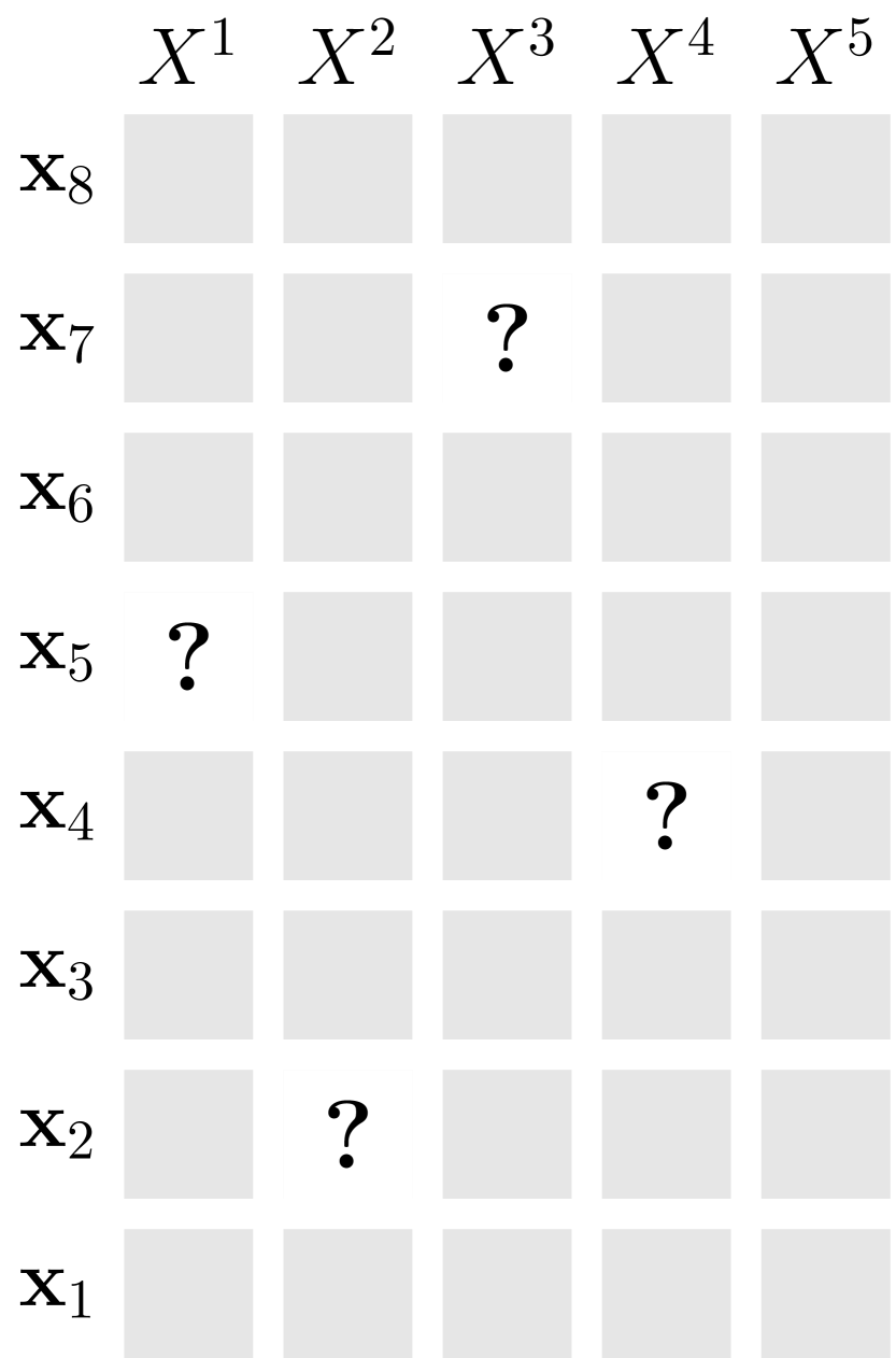
(a)

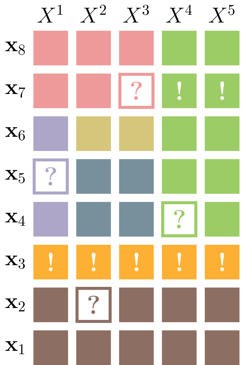
(b)

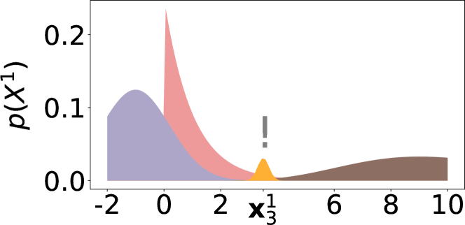
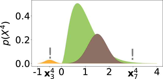
(c)

(d)

$$\mathcal{P}_{1}:5.9\leq \ {\color[rgb]{0.5546875,0.4296875,0.38671875}X^{1}}<10.0\ \wedge$$

$$1.0\leq \ {\color[rgb]{0.5546875,0.4296875,0.38671875}X^{4}}<2.01$$

$$(\mathsf{supp}( \mathcal{P}_{1})=0.25)$$

$$\mathcal{P}_{2}:(0.0\leq \ {\color[rgb]{0.9375,0.60546875,0.60546875}X^{1}}<3.5\ \vee$$

$$-2.0\leq \ {\color[rgb]{0.68359375,0.65234375,0.7890625}X^{1}}<2.0)\ \wedge$$

$$0.1\leq \ {\color[rgb]{0.61328125,0.80078125,0.39453125}X^{4}}<3.0$$

$$(\mathsf{supp}( \mathcal{P}_{2})=0.49)$$

(e)

Figure 1: Automatic exploratory analysis with ABDA on a tabular dataset comprising samples from mixed continuous and discrete features $\mathbf{X}=\{X^{1},\ldots,X^{5}\}$, potentially containing missing values (denoted as “$?$”) (1(a)). The latent dependency structure inferred by ABDA induces a hierarchical partition over samples and features (i.e., a hierarchical co-clustering) given a learned Sum-Product Network (SPN) structure (1(b)). Statistical data types and likelihood models are discovered by estimating each feature distribution as a mixture model over a dictionary of suitable and interpretable parametric model, e.g., Gaussian for real data, Gamma, Exponential distributions for positive data in (1(c)-1(d)). ABDA can efficiently impute missing entries as the most probable values 1(b) by SPN inference routines. Anomalous entries (denoted as “$!$” in 1(b)-1(c)), on the other hand, are presented to the user as low-likelihood samples that are relegated to micro-clusters (e.g., $\mathbf{x}_{3}$) or to the distribution tails (e.g., $\mathbf{x}_{7}^{4}$ and $\mathbf{x}_{7}^{5}$). Moreover, ABDA allows to automatically discover complex dependency patterns, e.g. conjunctions of confidence intervals, by exploiting the correlations over the induced hierarchical co-clustering (1(e)).

Unfortunately, classical approaches to DE, even if ubiquitous in ML applications, are still far from delivering automatic tools suitable for performing all these steps on real-world data. First, general-purpose density estimators usually assume the statistical data types and the likelihood models to be known a priori and homogeneous across random variables (RVs) or mixture model components [33]. Indeed, the standard approach is still to generally treat all continuous data as (mixtures of) Gaussian RVs and discrete data as categorical variables. Second, they either assume “shallow” dependency structures that might be too simplistic to capture real-world statistical dependencies or use “deeper” latent structures which cannot be easily learned. As a result, they generally lack enough flexibility to deal with fine grain statistical dependencies, and to be robust to corrupt data and outliers, especially when a maximum likelihood learning approach is used.

A Bayesian treatment of DE, on the other hand, often struggles to scale up to high-dimensional data and approximate inference routines are needed [15]. CrossCat [21] shows a clear example of this trade-off. Even though CrossCat models sub-populations in the data with context-specific latent variables, this latent structure is limited to a two-layer hierarchy, and even so inference routines have to be approximated for efficiency. Moreover, it is still limited to fixed and homogeneous statistical data types and therefore, likelihood models.

The latent variable matrix factorization model (ISLV) introduced in [33] is the first attempt to overcome this limitation by modeling uncertainty over the statistical data types of the features. However, like CrossCat, it can only perform inference natively in the transductive case, i.e., to data available during training. While ISLV allows one to infer the data type of a feature, this approach still uses a single ad-hoc likelihood function for each data type.

Recently, Mixed Sum-Product Networks (MSPNs) [23] have been proposed as deep models for heterogeneous data able to perform tractable inference also in the inductive scenario, i.e., on completely unobserved test data. Indeed, MSPNs can exploit context specific independencies to learn latent variable hierarchies that are deeper than CrossCat. However, MSPNs assume piecewise-linear approximations as likelihood models for both continuous and discrete RVs, which are not as interpretable as parametric distributions and also require continuous RVs to undergo a delicate discretization process. As a result, MSPNs are highly prone to overfitting, and learning them via maximum likelihood results into a lack of robustness.

In this paper, we leverage the above models’ advantages while addressing their shortcomings by proposing Automatic Bayesian Density Analysis (ABDA). Specifically, ABDA relies on sum-product networks (SPNs) to capture statistical dependencies in the data at different granularity through a hierarchical co-clustering. This rich latent structure is learned in an adaptive way, which automates the selection of adequate likelihood models for each data partition, and thus extends ISLV uncertainty modeling over statistical types. As a result, ABDA goes beyond standard density estimation approaches, qualifying as the first approach to fully automate exploratory analysis for heterogeneous tabular data at large.

As illustrated in Fig. 1, ABDA allows for:

i)

inference for both the statistical data types and (parametric) likelihood models;

ii)

robust estimation of missing values;

iii)

detection of corrupt or anomalous data;

iv)

automatic discovery of the statistical dependencies and local correlations in the data.

ABDA relies on Bayesian inference through Gibbs sampling, allowing us to robustly measure uncertainties at performing all the above tasks. In our extensive experimental evaluation, we demonstrate that ABDA effectively assists domain experts in both transductive and inductive settings. Supplementary material and a reference implementation of ABDA are available at github.com/probabilistic-learning/abda.

Sum-Product Networks (SPNs)

As SPNs provide the hierarchical latent backbone of ABDA, we will now briefly review them. Please refer to [25] for more details.

In the following, upper-case letters, e.g. $X$, denote RVs and lower-case letters their values, i.e., $x\sim X$. Similarly, we denote sets of RVs as $\mathbf{X}$, and their combined values as $\mathbf{x}$.

Representation.

An SPN $\mathcal{S}$ over a random vector $\mathbf{X}=\{X^{1},\ldots,X^{D}\}$ is a probabilistic model defined via a directed acyclic graph. Each leaf node $\mathsf{L}$ represents a probability distribution function over a single RV $X\in\mathbf{X}$, also called its scope. Inner nodes represent either weighted sums ($\mathsf{S}$) or products ($\mathsf{P}$). For inner nodes, the scope is defined as the union of the scopes of its children. The set of children of a node $\mathsf{N}$ is denoted by $\mathsf{ch}(\mathsf{N})$.

A sum node $\mathsf{S}$ encodes a mixture model $\mathcal{S}_{\mathsf{S}}(\mathbf{x})=\sum_{\mathsf{N}\in\mathsf{ch}(\mathsf{S})}\omega_{\mathsf{S},\mathsf{N}}\mathcal{S}_{\mathsf{N}}(\mathbf{x})$ over sub-SPNs rooted at its children $\mathsf{ch}(\mathsf{S})$. We require that the all children of a sum node share the same variable scope—this condition is referred to as completeness [27]. The weights of a sum $\mathsf{S}$ are drawn from the standard simplex (i.e., $\omega_{\mathsf{S},\mathsf{N}}\geq 0$, $\sum_{\mathsf{N}\in\mathsf{ch}(\mathsf{S})}\omega_{\mathsf{S},\mathsf{N}}=1$) and denoted as $\Omega^{\mathsf{S}}$. A product node $\mathsf{P}$ defines a factorization $\mathcal{S}_{\mathsf{P}}(\mathbf{x})=\prod_{\mathsf{N}\in\mathsf{ch}(\mathsf{P})}\mathcal{S}_{\mathsf{N}}(\mathbf{x})$ over its children distributions defined over disjoint scopes—this condition is referred to as decomposability [27]. The parameters of $\mathcal{S}$ are the set of sum weights $\bm{\Omega}=\{\Omega^{\mathsf{S}}\}_{\mathsf{S}\in\mathcal{S}}$ and the set of all leaf distribution parameters $\{\bm{H}_{\mathsf{L}}\}_{\mathsf{L}\in\mathcal{S}}$.

Complete and decomposable SPNs are highly expressive deep models and have been successfully employed in several ML domains [26, 22, 28, 35] to capture highly complex dependencies in real-world data. Moreover, they also allow to exactly evaluate complete evidence, marginal and conditional probabilities in linear time w.r.t. their representation size [7].

Latent variable representation.

Since each sum node defines a mixture over its children, one may associate a categorical latent variable (LV) $Z^{\mathsf{S}}$ to each sum $\mathsf{S}$ indicating a component. This results in a hierarchical model over the set of all LVs $\mathbf{Z}=\{Z^{\mathsf{S}}\}_{\mathsf{S}\in\mathcal{S}}$. Specifically, an assignment to $\mathbf{Z}$ selects an induced tree in $\mathcal{S}$ [37, 25, 36], i.e., a tree path $\mathcal{T}$ starting from the root and comprising exactly one child for each visited sum node and all child branches for each visited product node (in green in Fig. 2(b)).

It follows from completeness and decomposability that $\mathcal{T}$ selects a subset of $D$ leaves, in a one-to-one correspondence with $\mathbf{X}$. When conditioned on a particular $\mathcal{T}$, the SPN distribution factorizes as $\prod_{d}\mathsf{L}^{d}_{j^{d}}$, where $\mathsf{L}^{d}_{k}$ is the $k^{\text{th}}$ leaf for the $d^{\text{th}}$ RV, and $\mathbf{j}=\{j^{1},\dots,j^{D}\}$ are the indices of the leaves selected by $\mathcal{T}$. The overall SPN distribution can be written as a mixture of such factorized distributions, running over all possible induced trees [37].

We will use this hierarchical LV structure to develop an efficient Gibbs sampling scheme to perform Bayesian inference for ABDA.

SPN learning.

Existing SPN learning works focus on learning the SPN parameters given a structure [13, 31, 37] or jointly learn both the structure and the parameters [9, 10]. The latter approach has recently gained more attention since it automatically discovers the hierarchy over the LVs $\mathbf{Z}$ and admits greedy heuristic learning schemes leveraging the probabilistic semantics of nodes in an SPN [14, 29, 34]. These approaches recursively partition a data matrix in a top-down fashion, performing hierarchical co-clustering (partitioning over data samples and features). As the base step, they learn a univariate likelihood model for single features. Otherwise, they alternatively try to partition either the RVs (or features) into independent groups, inducing a product node; or the data samples (clustering), inducing a sum node.

ABDA resorts to the SPN learning approach employed by MSPNs [23], as it is the only one able to build an SPN structure in a likelihood-agnostic way, therefore being suitable for our heterogeneous setting. It performs a partitioning over mixed continuous and discrete data by exploiting a randomized approximation of the Hirschfeld-Gebelein-Rényi Maximum Correlation Coefficient (RDC) [20]. Note that, ABDA employs it to automatically select an initial, global, LV structure, to be later provided to its Bayesian inference routines.

Automatic Bayesian Density Analysis

For a general discussion, we extend $\mathbf{X}$ to a whole data matrix containing $N$ samples (rows) and $D$ features (columns). RVs which are local to a row (column) receive now a sub-script $n$ (super-script $d$).

Our proposed Automatic Bayesian Density Analysis (ABDA) model can be thought as being organized in two levels: a global level, capturing dependencies and correlations among the features, and a level which is local w.r.t. each feature, consisting of dictionaries of likelihood models for that feature. This model is illustrated Fig. 2, via its graphical model representation, and corresponding SPN representations. In this hierarchy, the global level captures context specific dependencies via recursive data partitioning, leveraging the LV structure of an SPN. The local level represents context-specific uncertainties about the variable types, conditioned on the global context.

In contrast to classical works on DE, where typically fixed likelihood models are used as mixture components, e.g., see [27, 34]), ABDA assumes a heterogeneous mixture model combining several likelihood models from a user-provided likelihood dictionary. This dictionary may contain likelihood models for diverse types of discrete (e.g. Poisson, Geometric, Categorical,…) and continuous (e.g., Gaussian, Gamma, Exponential,…) data. It can be built in a generous automatic way, incorporating arbitrary rich collections of domain-agnostic likelihood functions. Alternatively, its construction can be limited to a sensible subset of likelihood models reflecting domain knowledge, e.g. a Gompertz and Weibull distributions might be included by a user specifically dealing with demographics data.

In what follows, assume that for each feature $d$ we have readily selected a dictionary $\{p^{d}_{\ell}\}_{\ell\in\mathcal{L}^{d}}$ of likelihood models, indexed by some set $\mathcal{L}^{d}$. We next describe the process generating $\mathbf{X}$, also depicted in Fig. 2(a), in detail.

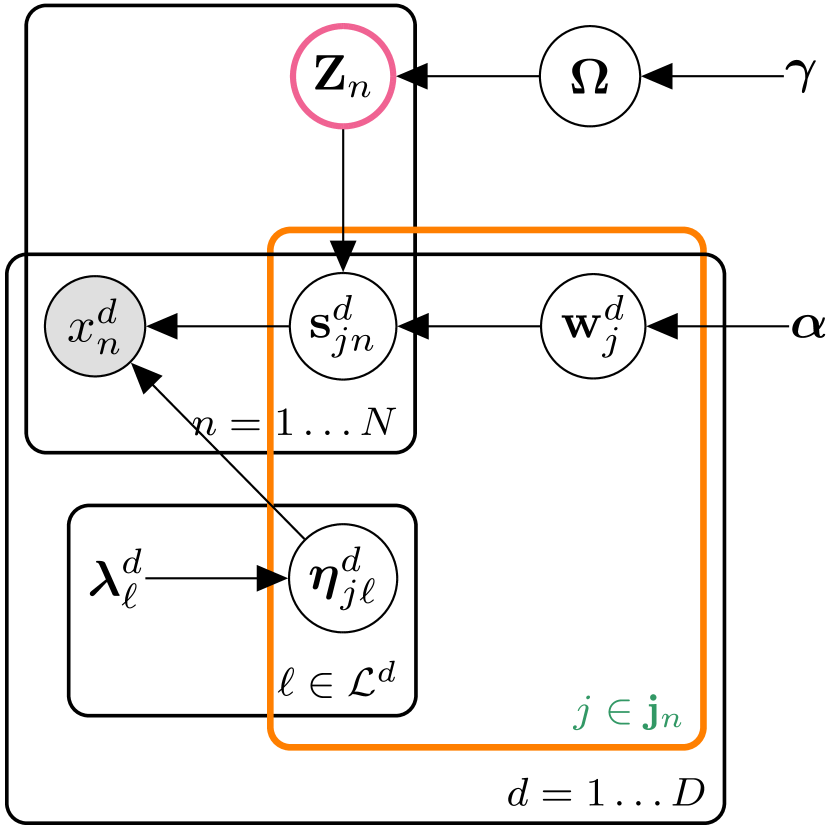
(a) Graphical model

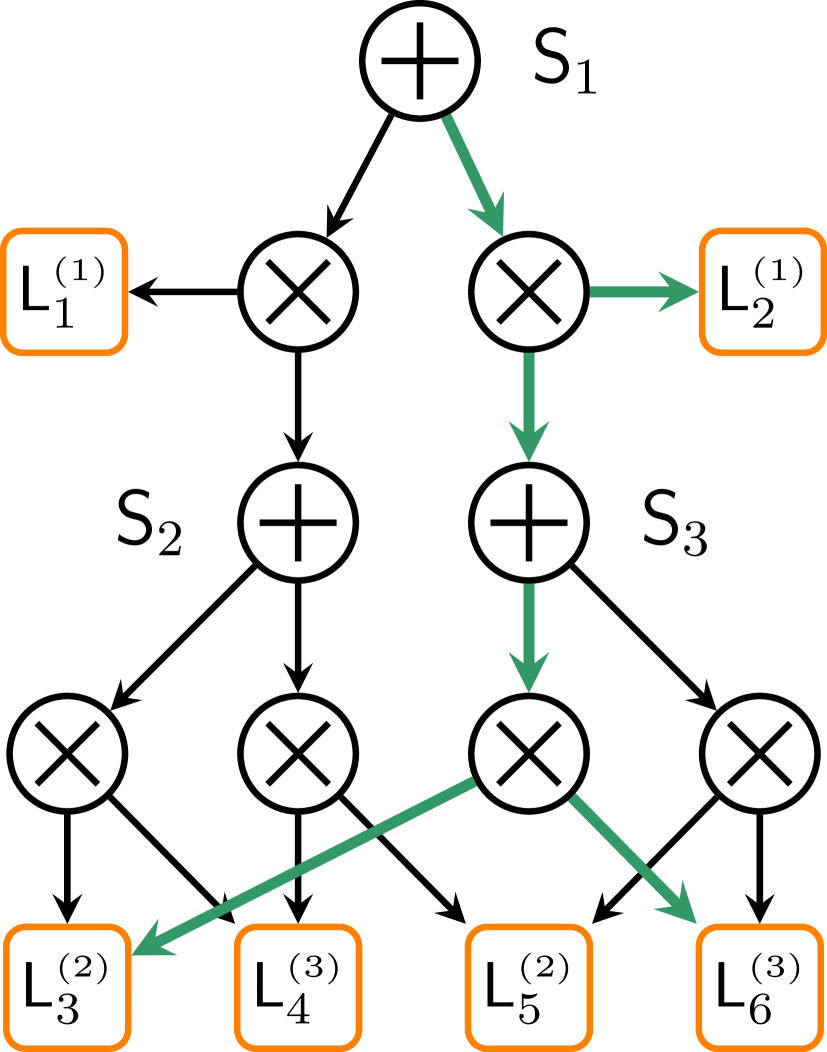
(b) SPN

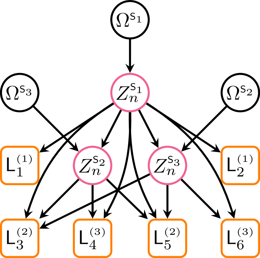
(c) LV interpretation

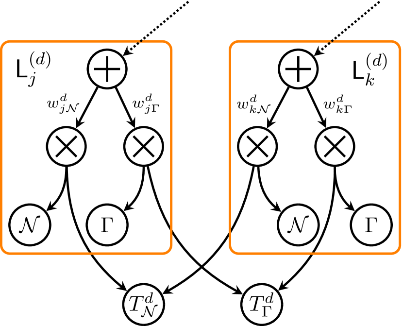
(d) Type-augmented SPN

Figure 2: (2(a)) Plate representation of ABDA, showing the global LV (pink) and local (orange) levels. (2(b)) The SPN representation with likelihood-modeling leaves $L_{j}^{(d)}$ over features $d$=1,2,3 selected by an induced tree (green), (2(c)) and its corresponding hierarchy over LVs $\mathbf{Z}$. (2(d)) A global mixture model over Gaussian ($\mathcal{N}$) and Gamma ($\Gamma$) likelihoods interpreted as sub-SPNs sharing global auxiliary LVs $T^{d}$ across the local likelihood mixture models for feature $d$.

Generative model.

The global level of ABDA contains latent vectors $\mathbf{Z}_{n}$ for each sample $\mathbf{x}_{n}$, associated with the SPN sum nodes (see previous section). Each LV $Z^{\mathsf{S}}_{n}$ in $\mathbf{Z}_{n}$ is drawn according to the sum-weights $\Omega^{\mathsf{S}}\in\bm{\Omega}$, which are associated a Dirichlet prior, parameterized with hyper-parameters $\bm{\gamma}$:

$$Z^{\mathsf{S}}_{n}\sim\mathsf{Cat}(\Omega^{\mathsf{S}}),\quad\quad\Omega^{\mathsf{S}}\sim\mathsf{Dir}(\bm{\gamma})$$

.

As previously discussed, an assignment of $\mathbf{Z}_{n}$ determines an induced tree through the SPN, selecting a set of indices $\mathbf{j}_{n}=(j^{1}_{n},\dots,j^{D}_{n})$, such that the joint distribution of $\mathbf{x}_{n}=(x_{n}^{1},\ldots,x_{n}^{D})$ factorizes as

$$p(\mathbf{x}_{n}\,|\,\mathbf{j}_{n},\bm{\eta})=\prod\nolimits_{d=1}^{D}\mathsf{L}^{d}_{j^{d}_{n}}(x_{n}^{d}\,|\,\bm{\eta}^{d}_{j^{d}_{n}}),$$ (1)

where $\mathsf{L}^{d}_{j}$ is the $j^{\text{th}}$ leaf for feature $d$ and $\bm{\eta}^{d}_{j}=\{\bm{\eta}^{d}_{j,\ell}\}_{\ell\in\mathcal{L}^{d}}$ is the set of parameters belonging to the likelihood models associated to it. More precisely, the $j^{\text{th}}$ leaf distribution $\mathsf{L}^{d}_{j}$ is modeled as a mixture over the likelihood dictionaries provided by the user, i.e.,

$$\mathsf{L}^{d}_{j}(x^{d}_{n}\,|\,\bm{\eta}^{d}_{j})=\sum\nolimits_{\ell\in\mathcal{L}^{d}}w^{d}_{j,\ell}\,p^{d}_{\ell}(x^{d}_{n}\,|\,\bm{\eta}^{d}_{j,\ell}).$$ (2)

Note that the likelihood models $p^{d}_{\ell}$ are shared among all leaves with the same scope $d$, but each leaf has its private parameter $\bm{\eta}^{d}_{j,\ell}$ for it. Moreover, each $\bm{\eta}^{d}_{j,\ell}$ is also equipped with a suitable prior distribution parameterized with hyper-parameters $\bm{\lambda}^{d}_{\ell}$. For a discussion on the selection of suitable prior distributions, refer to Appendix B in the supplementary material.

The likelihood mixture coefficients ${w}_{j,\ell}^{d}$ are drawn from a Dirichlet distribution with hyper-parameters $\bm{\alpha}$, i.e., $\mathbf{w}^{d}_{j}\sim\mathsf{Dir}(\bm{\alpha})$. For each entry $x_{n}^{d}$, the likelihood model is selected by an additional categorical LV $s_{j,n}^{d}\sim\mathsf{Cat}(\mathbf{w}^{d}_{j})$. Finally, the observation entry $x_{n}^{d}$ is sampled from the selected likelihood model: $x_{n}^{d}\sim p^{d}_{s_{j,n}^{d}}$.

Bayesian Inference

The hierarchical LV structure of SPNs allows ABDA to perform Bayesian inference via a simple and effective Gibbs sampling scheme. To initialize the global structure, we use the likelihood-agnostic SPN structure learning algorithm proposed for MSPNs [23]. Specifically, we apply the RDC to split samples and features while extending it to deal with missing data (see supplementary for details). The local level in ABDA is constructed by equipping each leaf node in $\mathcal{S}$ with the dictionaries of likelihood models as described above. Additionally, one can introduce global type-RVs, responsible for selecting a specific likelihood model (or data type) for each feature $d$ (see Fig. 2(d) and further explanations below).

Furthermore note that, in contrast to MSPNs, ABDA is not constrained to the LV structure provided by structure learning. Indeed, inference in ABDA accounts for uncertainty also on the underlying latent structure. As a consequence, a wrongly overparameterized LV structure provided to ABDA can still be turned into a simpler one by our algorithm by using a sparse prior on the SPN weights (see Appendix H).

To perform inference, we draw samples $\mathcal{D}$ from the posterior distribution $p(\mathbf{Z},\mathbf{s},\bm{\Omega},\mathbf{w},\bm{\eta}\,|\,\mathbf{X})$ via Gibbs sampling, where $\mathbf{Z}$ is the set of the SPN’s LVs, $\mathbf{s}$ is the set of all local LVs selecting the likelihood models, $\bm{\Omega}$ is the set of all sum-weights, $\mathbf{w}$ are the distributions of $\mathbf{s}$, and $\bm{\eta}$ is the set collecting all parameters of all likelihood models. Next, we describe each routine involved to sample from the conditionals for each of these RVs in turn. Algorithm 1 summarizes the full Gibbs sampling scheme. Improved mixing via a Rao-Blackwellised version of the proposed sampler is discussed in Appendix A.

Sampling LVs $\mathbf{Z}$.

Given the hierarchical LV structure of $\mathcal{S}$, it is easy to produce a sample for $\mathbf{Z}_{n}$ by ancestral sampling, i.e. by sampling an induced tree $\mathcal{T}_{n}$. To this end we condition on a sample $\mathbf{x}_{n}$, and current $\bm{\Omega}$, $\bm{\eta}$ and $\mathbf{w}$. Starting from the root of $\mathcal{S}$, for each sum node $\mathsf{S}$ we encounter, we sample a child branch $c$ from

$$p(Z_{n}^{\mathsf{S}}=c\,|\,,\mathbf{x}_{n},\bm{\Omega},\bm{\eta},\mathbf{w})\propto\omega_{\mathsf{S},c}\,\mathcal{S}_{c}(\mathbf{x}_{n}\,|\,\bm{\Omega},\bm{\eta},\mathbf{w}).$$ (3)

Note that we are effectively conditioning on the states of the ancestors of $\mathsf{S}$. Moreover, we have marginalized out all $\bm{Z}$ below $\mathsf{S}$ and all $\bm{s}$, which just amounts to evaluating $\mathcal{S}_{c}$ bottom-up, for given parameters $\bm{\Omega}$, $\bm{\eta}$, and $\mathbf{w}$ [27].

Note that, in general, sampling a tree $\mathcal{T}_{n}$ does not reach all sum nodes. Since these sum nodes are “detached” from the data, we need to sample their LVs from the prior [25].

Sampling likelihood model assignments $\mathbf{s}$.

Similarly as for LVs $\mathbf{Z}_{n}$, we sample $s_{j,n}^{d}$ from the posterior distribution $p(s_{j,n}^{d}=\ell\,|\,\mathbf{w},\mathbf{j},\bm{\eta})\propto w_{j,\ell}^{d}\,p^{d}_{\ell}(x_{n}^{d}\,|\,\bm{\eta})$ if $j=j^{d}_{n}$.

Sampling leaf parameters $\bm{\eta}$.

Sampling $\mathbf{Z}_{n}$ gives rise to the leaf indices $\mathbf{j}_{n}$, which assign samples to leaves. Within leaves, $\mathbf{s}$ further assign samples to likelihood models. For parameters $\bm{\eta}^{d}_{j,\ell}$ let $\mathbf{X}^{d}_{j,\ell}=\{x^{d}_{n}\,|\,\forall n\colon j^{d}_{n}=j\wedge s^{d}_{j,n}=\ell\}$, i.e., the samples in the $d^{\text{th}}$ column of $\mathbf{X}$ which have been assigned to the $\ell^{\text{th}}$ model in leaf $\mathsf{L}^{d}_{j}$. Then, $\bm{\eta}^{d}_{j,\ell}$ is updated according to

$$\bm{\eta}^{d}_{j,\ell}\sim\prod_{x\in\mathbf{X}^{d}_{j,\ell}}p^{d}_{\ell}(x\,|\,\bm{\eta}^{d}_{j,\ell})\,p(\bm{\eta}^{d}_{j,\ell}\,|\,\bm{\lambda}_{\ell}^{d}).$$

When the likelihood models $p^{d}_{\ell}$ are equipped with conjugate priors, these updates are straightforward. Moreover, also for non-conjugate priors they can easily be approximated using numerical methods, since we are dealing with single-dimensional problems.

Sampling weights $\bm{\Omega}$ and $\mathbf{w}$.

For each sum node $\mathsf{S}$ we sample its associated weights from the posterior $p(\Omega^{\mathsf{S}}\,|\,\{\mathbf{Z}_{n}\}_{n=1}^{N})$, which is a Dirichlet distribution with parameters $\bm{\gamma}+\sum_{n=1}^{N}\mathds{1}\{(\mathsf{S},c)\in\mathcal{T}_{{n}}\}$. Similarly, we can sample the likelihood weights $\mathbf{w}^{d}_{j}$ from a Dirichlet distribution with parameters $\bm{\alpha}+[\sum_{n=1}^{N}\mathds{1}\{j^{d}_{n}=j\wedge s_{j,n}^{d}=\ell\}]_{\ell\in\mathcal{L}^{d}}$.

Automating exploratory data analysis

In this section, we discuss how inference in ABDA can be exploited to perform common exploratory data analysis tasks in an automatic way. For all inference tasks (e.g., computing $\log p(\mathbf{x}_{n})$), one can either condition on the model parameters, e.g., by using the maximum likelihood parameters within posterior samples $\mathcal{D}$, or perform a Monte Carlo estimate over $\mathcal{D}$. While the former allows for efficient computations, the latter allows for quantifying the model uncertainty. We refer to Appendixes E-G in the supplementary for more details.

Missing value imputation.

Given a sample $\mathbf{x}_{n}=(\mathbf{x}_{n}^{o},\mathbf{x}_{n}^{m})$ comprising observed $\mathbf{x}_{n}^{o}$ and missing $\mathbf{x}^{m}_{n}$ values, ABDA can efficiently impute the latter as the most probable explanation $\tilde{\mathbf{x}}_{n}^{m}=\operatorname{\arg\max}_{\mathbf{x}_{n}^{m}}\mathcal{S}(\mathbf{x}_{n}^{m}|\mathbf{x}_{n}^{o})$ via efficient approximate SPN routines [25].

Anomaly detection.

ABDA is robust to outliers and corrupted values since, during inference, it will tend to assign anomalous samples into low-weighted mixture components, i.e., sub-networks of the underlying SPN or leaf likelihood models. Outliers will tend to be either grouped into anomalous micro-clusters [4] or assigned to the tails of a likelihood model.

Therefore, $\log p(\mathbf{x}_{n})$ can be used as a strong signal to indicate $\mathbf{x}_{n}$ is an outlier (in the transductive case) or a novelty (in the inductive case) [17].

Data type and likelihood discovery.

ABDA automatically estimates local uncertainty over likelihood models and statistical types by inferring the dictionary coefficients $w^{d}_{j,\ell}$ for a leaf $\mathsf{L}^{d}_{j}$.

However, we can extend ABDA to reason about data type also on a global level by explicitly introducing a type variable $T^{d}$ for feature $d$. This type variable might either represent a parametric type, e.g., Gaussian or Gamma, or a data type, e.g., real-valued or positive-real-valued, in a similar way to ISLV [33]. To this end, we introduce state-indicators for each type variable $T^{d}$, and connect them into each likelihood model in leaf $\mathsf{L}^{d}_{j}$, as shown in Fig. 2(d). In this example, we introduced the state-indicators $T^{d}_{\mathcal{N}}$ and $T^{d}_{\Gamma}$ to represent a global type $T^{d}$ which distinguishes between Gaussian and Gamma distribution.

Note that this technique is akin to the augmentation of SPNs [25], i.e., explicitly introducing the LVs for sum nodes. Here, however, the introduced $\{T^{d}\}_{d=1}^{D}$ have an explicit intended semantic as global data type variables. Crucially, after introducing $\{T^{d}\}_{d=1}^{D}$, the underlying SPN is still complete and decomposable, i.e., we can easily perform inference over them. In particular, we can estimate the posterior probability for a feature $d$ to have a particular type as:

$$p(T^{d}\,|\,\mathbf{X})\approx\frac{1}{|\mathcal{D}|}\sum_{\{\bm{\Omega},\mathbf{w},\bm{\eta}\}\in\mathcal{D}}\mathcal{S}(T^{d}\,|\,\Omega,\mathbf{w},\bm{\eta}).$$ (4)

The marginal terms $\mathcal{S}(T^{d}\,|\,\Omega,\mathbf{w},\bm{\eta})$ are easily obtained via SPN inference – we simply need to set all leaves and all indicators for $\{T^{d^{\prime}}\}_{d^{\prime}\not=d}$ equal to $1$ [27].

Dependency pattern mining.

ABDA is able to retrieve global dependencies, e.g., by computing pairwise hybrid mutual information, in a similar way to MSPNs [23].

Additionally, ABDA can provide users local patterns in the form of dependencies within a data partition $\mathbf{X}^{\mathsf{N}}\subseteq\mathbf{X}$ associated with any node $\mathsf{N}$ in $\mathcal{S}$. In particular, let $\mathbf{X}^{\mathsf{N}}$ contain all entries $x^{d}_{n}$ such that $d$ is in the scope of $\mathsf{N}$ and $n$ such that $\mathbf{Z}_{n}$ yield an induced tree from the SPN’s root to $\mathsf{N}$. Then, for each leaf $\mathsf{L}^{d}_{j}$ and likelihood model $\ell\in\mathcal{L}^{d}$ one can extract a pattern of the form $\mathcal{P}\colon\pi_{l}^{d}\leq X^{d}<\pi_{h}^{d}$, where $[\pi_{l}^{d},\pi_{h}^{d})$ is an interval in the domain of $X^{d}$. The pattern can be deemed as present, when its probability exceeds a user-defined threshold $\theta$: $p_{\mathsf{L}^{d}_{j}}(\mathcal{P})\geq\theta$.

A conjunction of patterns $\mathcal{P}^{\mathsf{N}}=\mathcal{P}_{1}\wedge\ldots\wedge\mathcal{P}_{|\mathsf{sc}(\mathsf{N})|}$ represents the correlation among features in $\mathbf{X}^{\mathsf{N}}$, and its relevance can be quantified as $p_{\mathcal{S}}(\mathcal{P}^{\mathsf{N}})$. This technique relates to the notion of support in association rule mining [1], whose binary patterns are here generalized to also support continuous and (non-binary) discrete RVs.

Experimental evaluation

We empirically evaluate ABDA on synthetic and real-world datasets both as a density estimator and as a tool to perform several exploratory data analysis tasks. Specifically, we investigate the following questions:

(Q1)

How does ABDA estimate likelihoods and statistical data types when a ground truth is available?

(Q2)

How accurately does ABDA perform density estimation and imputation over unseen real-world data?

(Q3)

How robust is ABDA w.r.t. anomalous data?

(Q4)

How can ABDA be exploited to unsupervisedly extract dependency patterns?

Experimental setting

In all experiments, we use a symmetric Dirichlet prior with $\gamma=10$ for sum weights $\bm{\Omega}$ and a sparse symmetric prior with $\alpha=0.1$ for the leaf likelihood weights $\mathbf{w}_{j}^{d}$. We consider the following likelihoods for continuous data: Gaussian distributions ($\mathcal{N}$) for $\mathsf{REAL}$-valued data; Gammas ($\Gamma$) and exponential ($\mathsf{Exp}$) for $\mathsf{POS}$itive real-valued data; and, for discrete data, we consider Poisson ($\mathsf{Poi}$) and Geometric ($\mathsf{Geo}$) distributions for $\mathsf{NUM}$erical data, and Categorical ($\mathsf{Cat}$) for $\mathsf{NOM}$inal data, while a Bernoulli for Binary data in the outlier detection case. For details on the prior distributions employed, for the likelihood parameters and their hyper-parameters, please refer to the Appendix.

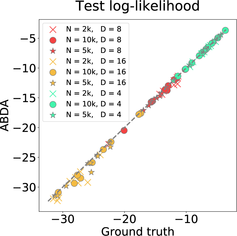
(a)

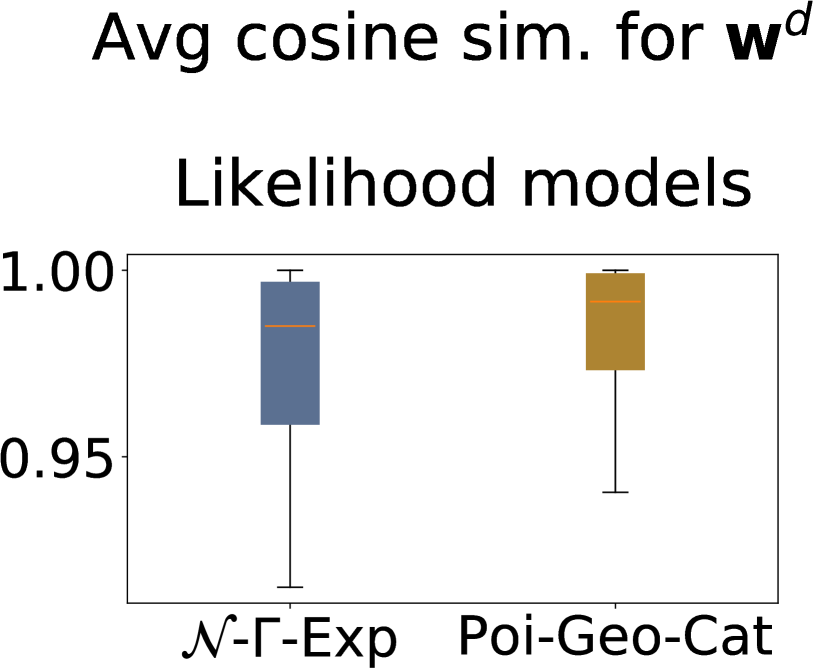
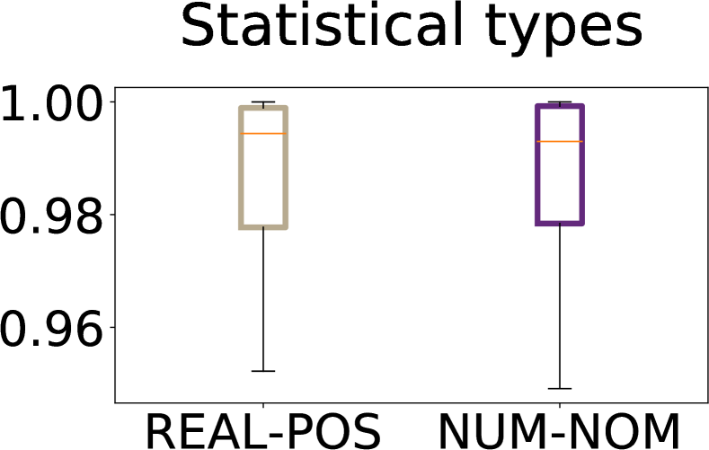
(b)

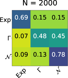
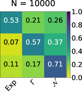
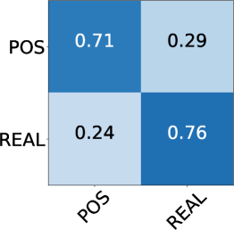
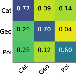
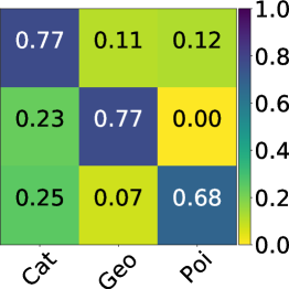
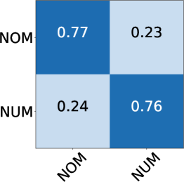
(c)

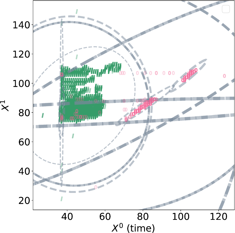
(d)

Figure 3: (3(a)) Mean test log-likelihood on synthetic data w.r.t. the ground truth. (3(b)) Distributions of the mean cosine similarity between true and retrieved uncertainty weights over likelihood models (top) and statistical types (bottom). (3(c)) Confusion matrices for the most likely likelihood model resp. statistical type. (3(d)) ABDA separates outliers (pink ‘O’) from inliers (green ‘I’) via hierarchical partitioning on Shuttle data, see Appendix F. Best viewed in colors.

Table 1: Density estimation. Mean test log-likelihood on real-world benchmark datasets for trans-/inductive scenarios. Best values are bold.

	transductive setting (10% mv)			transductive setting (50% mv)			inductive setting
	ISLV	ABDA	MSPN	ISLV	ABDA	MSPN	ABDA	MSPN
Abalone	-1.15$\scriptstyle\scriptstyle\pm 0.12$	-0.02$\scriptstyle\pm 0.03$	0.20	-0.89$\scriptstyle\pm 0.36$	-0.05$\scriptstyle\pm 0.02$	0.14	2.22$\scriptstyle\pm 0.02$	9.73
Adult	-	-0.60$\scriptstyle\pm\mathbf{0.02}$	-3.46	-	-0.69$\scriptstyle\pm\mathbf{0.01}$	-5.83	-5.91$\scriptstyle\pm\mathbf{0.01}$	-44.07
Austral.	-7.92$\scriptstyle\pm 0.96$	-1.74$\scriptstyle\pm\mathbf{0.19}$	-3.85	-9.37$\scriptstyle\pm 0.69$	-1.63$\scriptstyle\pm\mathbf{0.04}$	-3.76	-16.44$\scriptstyle\pm\mathbf{0.04}$	-36.14
Autism	-2.22$\scriptstyle\pm 0.06$	-1.23$\scriptstyle\pm\mathbf{0.02}$	-1.54	-2.67$\scriptstyle\pm 0.16$	-1.24$\scriptstyle\pm\mathbf{0.01}$	-1.57	-27.93$\scriptstyle\pm\mathbf{0.02}$	-39.20
Breast	-3.84$\scriptstyle\pm 0.05$	-2.78$\scriptstyle\pm 0.07$	-2.69	-4.29$\scriptstyle\pm 0.17$	-2.85$\scriptstyle\pm\mathbf{0.01}$	-3.06	-25.48$\scriptstyle\pm\mathbf{0.05}$	-28.01
Chess	-2.49$\scriptstyle\pm 0.04$	-1.87$\scriptstyle\pm\mathbf{0.01}$	-3.94	-2.58$\scriptstyle\pm 0.04$	-1.87$\scriptstyle\pm\mathbf{0.01}$	-3.92	-12.30$\scriptstyle\pm\mathbf{0.00}$	-13.01
Crx	-12.17$\scriptstyle\pm 1.41$	-1.19$\scriptstyle\pm\mathbf{0.12}$	-3.28	-11.96$\scriptstyle\pm 1.01$	-1.20$\scriptstyle\mathbf{\pm}\mathbf{0.04}$	-3.51	-12.82$\scriptstyle\pm\mathbf{0.07}$	-36.26
Dermat.	-2.44$\scriptstyle\pm 0.23$	-0.96$\scriptstyle\pm\mathbf{0.02}$	-1.00	-3.57$\scriptstyle\pm 0.32$	-0.99$\scriptstyle\pm\mathbf{0.01}$	-1.01	-24.98$\scriptstyle\pm\mathbf{0.19}$	-27.71
Diabetes	-10.53$\scriptstyle\pm 1.51$	-2.21$\scriptstyle\pm\mathbf{0.09}$	-3.88	-12.52$\scriptstyle\pm 0.52$	-2.37$\scriptstyle\pm\mathbf{0.09}$	-4.01	-17.48$\scriptstyle\pm\mathbf{0.05}$	-31.22
German	-3.49$\scriptstyle\pm 0.21$	-1.54$\scriptstyle\pm\mathbf{0.01}$	-1.58	-4.06$\scriptstyle\pm 0.28$	-1.55$\scriptstyle\pm\mathbf{0.01}$	-1.60	-25.83$\scriptstyle\pm\mathbf{0.05}$	-26.05
Student	-2.83$\scriptstyle\pm 0.27$	-1.56$\scriptstyle\pm\mathbf{0.03}$	-1.57	-3.80$\scriptstyle\pm 0.29$	-1.57$\scriptstyle\pm\mathbf{0.01}$	-1.58	-28.73$\scriptstyle\pm\mathbf{0.10}$	-30.18
Wine	-1.19$\scriptstyle\pm 0.02$	-0.90$\scriptstyle\pm 0.02$	-0.13	-1.34$\scriptstyle\pm 0.01$	-0.92$\scriptstyle\pm 0.01$	-0.41	-10.12$\scriptstyle\pm 0.01$	-0.13

Table 2: Anomaly detection with ABDA. Mean test log-likelihood on real-world benchmark datasets for trans-/inductive scenarios. Best values are bold.

outlier detection
	1SVM	LOF	HBOS	ABDA
Aloi	51.71$\scriptstyle\scriptstyle\pm 0.02$	74.19$\scriptstyle\scriptstyle\pm 0.70$	52.86$\scriptstyle\scriptstyle\pm 0.53$	47.20$\scriptstyle\scriptstyle\pm 0.02$
Thyroid	46.18$\scriptstyle\scriptstyle\pm 0.39$	62.38$\scriptstyle\scriptstyle\pm 1.04$	62.77$\scriptstyle\scriptstyle\pm 3.69$	84.88$\scriptstyle\scriptstyle\pm 0.96$
Breast	45.77$\scriptstyle\scriptstyle\pm 11.1$	98.06$\scriptstyle\scriptstyle\pm 0.70$	94.47$\scriptstyle\scriptstyle\pm 0.79$	98.36$\scriptstyle\scriptstyle\pm 0.07$
Kdd99	53.40$\scriptstyle\scriptstyle\pm 3.63$	46.39$\scriptstyle\scriptstyle\pm 1.95$	87.59$\scriptstyle\scriptstyle\pm 4.70$	99.79$\scriptstyle\scriptstyle\pm 0.10$
Letter	63.38$\scriptstyle\scriptstyle\pm 17.6$	86.55$\scriptstyle\scriptstyle\pm 2.23$	60.47$\scriptstyle\scriptstyle\pm 1.80$	70.36$\scriptstyle\scriptstyle\pm 0.01$
Pen-glo	46.86$\scriptstyle\scriptstyle\pm 1.02$	87.25$\scriptstyle\scriptstyle\pm 1.94$	71.93$\scriptstyle\scriptstyle\pm 1.68$	89.87$\scriptstyle\scriptstyle\pm 2.87$
Pen-loc	44.11$\scriptstyle\scriptstyle\pm 6.07$	98.72$\scriptstyle\scriptstyle\pm 0.20$	64.30$\scriptstyle\scriptstyle\pm 2.70$	90.86$\scriptstyle\scriptstyle\pm 0.79$
Satellite	52.14$\scriptstyle\scriptstyle\pm 3.08$	83.51$\scriptstyle\scriptstyle\pm 11.98$	90.92$\scriptstyle\scriptstyle\pm 0.16$	94.55$\scriptstyle\scriptstyle\pm 0.68$
Shuttle	89.37$\scriptstyle\scriptstyle\pm 5.13$	66.29$\scriptstyle\scriptstyle\pm 1.69$	98.47$\scriptstyle\scriptstyle\pm 0.24$	78.61$\scriptstyle\scriptstyle\pm 0.02$
Speech	45.61$\scriptstyle\scriptstyle\pm 3.64$	49.37$\scriptstyle\scriptstyle\pm 0.87$	47.47$\scriptstyle\scriptstyle\pm 0.10$	46.96$\scriptstyle\scriptstyle\pm 0.01$

(Q1) Likelihood and statistical type uncertainty

We use synthetic data in order to have control over the ground-truth distribution of the data. To this end, we generate 90 synthetic datasets with different combinations of likelihood models and dependency structures with different numbers of samples $N\in\{2000,5000,10000\}$ and numbers of features $D\in\{4,8,16\}$. For each possible combination of values, we create ten independent datasets of $N$ samples (reserving $20\%$ of them for testing), yielding $90$ data partitionings randomly built by mimicking the SPN learning process of [14, 34]. The leaf distributions have been randomly drawn from the aforementioned likelihood dictionaries. We then perform density estimation with ABDA on these datasets. See Appendix C for details on ABDA inference and the data generation process.

Fig. 8 summarizes our results. In Fig. 3(a) we see that ABDA’s likelihood matches the true model closely in all settings, indicating that ABDA is an accurate density estimator. Additionally, as shown in Fig. 3(b), ABDA is able to capture the uncertainty over data types, as it achieves high average cosine similarity between the ground truth type distribution and the inferred posterior over data type $p(T^{d}\,|\,\mathbf{X})$ (see Eq. (4)), both for i) likelihood functions (using $\mathcal{N}$, $\Gamma$ and $\mathsf{Exp}$ for continuous and $\mathsf{Pos}$, $\mathsf{Geo}$ and $\mathsf{Cat}$ for discrete features); and ii) the corresponding statistical data types (using $\mathsf{POS}$ and $\mathsf{REAL}$ for continuous and $\mathsf{NUM}$ and $\mathsf{NOM}$ for discrete features).

Furthermore, when forcing a hard decision on distributions and data types, ABDA delivers accurate predictions. As shown in the confusion matrices in Fig. 3(c), selecting the most probable likelihood (data type) based on ABDA inference matches the ground truth up to the expected indiscernibility due to finite sample size. For further discussions, please refer to [33].

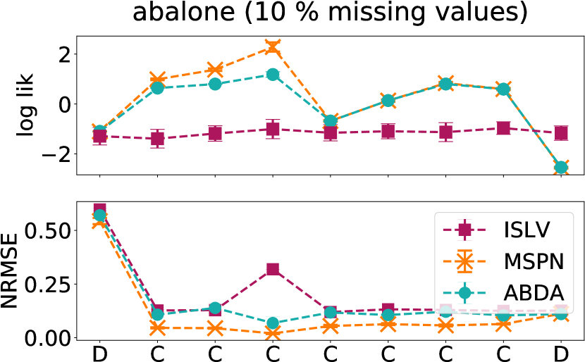
(a) Abalone

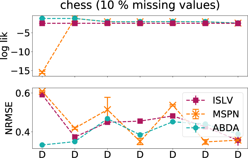
(b) Chess

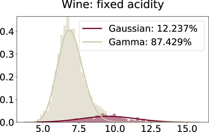
(c)

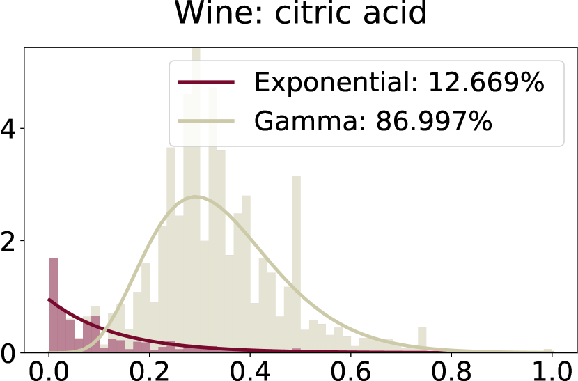
(d)

Figure 4: Left (a, b): Missing data estimation. Feature-wise test log-likelihood (top) and NRMSE (bottom) for 10% of missing values for ABDA (cyan) ISLV (purple) and MSPN (orange). Features on the x-axis are labeled as ($\mathsf{D}$)iscrete or ($\mathsf{C}$)ontinuous. More plots in Appendix E.
Right (c, d): Data exploration and dependency discovery with ABDA on the Wine quality dataset. ABDA identifies the two modalities in the data induced by red and white wines, and extracts the following patterns: $5.8\leq{\color[rgb]{0.80078125,0.79296875,0.6640625}\mathsf{FixAcid}}<8.1\wedge 0.2\leq{\color[rgb]{0.80078125,0.79296875,0.6640625}\mathsf{CitAcid}}<0.5$ and $7.1\leq{\color[rgb]{0.46484375,0.0390625,0.17578125}\mathsf{FixAcid}}<12.0\wedge 0.0\leq{\color[rgb]{0.46484375,0.0390625,0.17578125}\mathsf{CitAcid}}<0.3$ ($\theta=0.9$).

(Q2) Density estimation and imputation

We evaluate ABDA both in a transductive scenario, where we aim to estimate (or even impute) the missing values in the data used for inference/training; and in an inductive scenario, where we aim to estimate (impute) data that was not available during inference/training. We compare against ISLV [33], which directly accounts for data type (but not likelihood model) uncertainty, and MSPNs [23], to observe the effect of modeling uncertainty over the RV dependency structure via an SPN LV hierarchy.

From ISLV and MSPN original works we select 12 real-world datasets differing w.r.t. size and feature heterogeneity. Appendix C reports detailed dataset information, while Appendix H contains additional experiments in the MSPN original setting. Specifically, for the transductive setting, we randomly remove either 10% or 50% of the data entries, reserving an additional 2% as a validation set for hyperparameter tuning (when required), and repeating five times this process for robust evaluation. For the inductive scenario, we split the data into train, validation, and test (70%, 10%, and 20% splits).

For ABDA and ISLV, we run 5000 iteratations of Gibbs sampling , discarding the first 4000 for burn-in. We set for ISLV the number of latent factors to $\lfloor D/2\rfloor$. We learn MSPNs with the same hyper-parameters as for ABDA structure learning, i.e., stopping to grow the network when the data to be split is less than 10% of the dataset, while employing a grid search in $\{0.3,0.5,0.7\}$ for the RDC dependency test threshold.

Tab. 1 reports the mean test-log likelihoods–evaluated on missing values in the transductive or on completely unseen test samples in the inductive cases–for all datasets. Here, we can see that ABDA outperforms both ISLVs and MSPNs in most cases for both scenarios. Moreover, since aggregated evaluations of heterogeneous likelihoods might be dominated by a subset features, we also report in Fig 4 the average test log-likelihood and the normalized root mean squared error (NRMSE) of the imputed missing values (normalized by the range of each RV separately) for each feature in the data. Here, we observe that ABDA is, in general, more accurate and robust across different features and data types than competitors. We finally remark that due to the piecewise approximation of the likelihood adopted by the MSPN, evaluations of the likelihood provided by this approach might be boosted by the fact that it renormalizes an infinite support distribution to a bounded one.

(Q3) Anomaly detection.

We follow the unsupervised outlier detection experimental setting in [17] to evaluate the ability of ABDA to detect anomalous samples on a set of standard benchmarks. As a qualitative example, we can observe in Fig 3(d) that ABDA either clusters outliers together or relegates them to leaf distribution tails, assigning them low probabilities. Tab. 1 compares, in terms of the mean AUC ROC, ABDA—for which we use the negative log-likelihood as the outlier score—with staple outlier detection methods like one-class SVMs (1SVM) [30], local outlier factor (LOF) [2] and histogram-based outlier score (HBOS) [16].

It is clearly visible that ABDA perform as good as—or even better—in most cases than methods tailored for outlier detection and not being usable for other data analysis tasks. Refer to Appendix F for further experimental details and results.

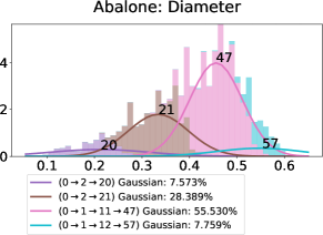
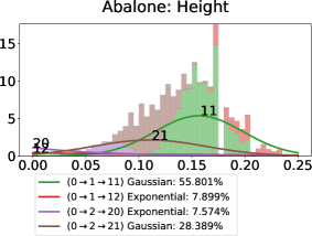
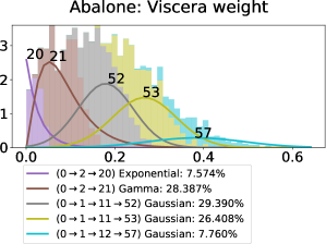
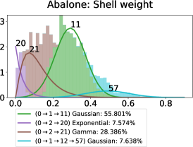
Figure 5: Data exploration and pattern discovery on the Abalone dataset, comprising physical measurements (e.g. diameter, height, weight) of different specimens. Each colored density belongs to a unique partition $\mathbf{X}^{\mathsf{N}}$ discovered by ABDA and here labeled by an integer indicating the corresponding node $\mathsf{N}$ (0 indicates the root of the SPN). Hierarchies over partitions are shown in the legend as the path connecting the root node to $\mathsf{N}$ (e.g., $0\rightarrow 1\rightarrow 11\rightarrow 47$ indicates that the partition #11 (green) is responsible for the green densities and it decomposes into the partitions #52 (gray), #53 (yellow) and #47 (pink), highlighting different correlation patterns across feature intervals). For instance, $\mathcal{P}_{1}:\quad 0.088\leq{\color[rgb]{0.171875,0.62890625,0.171875}\mathsf{Height}}<0.224\quad\wedge 0.158\leq{\color[rgb]{0.171875,0.62890625,0.171875}\mathsf{ShellWeight}}<0.425\quad(supp(\mathcal{P}_{1})=0.507)$ is a pattern within such a partition, correlating the height and the shell weight features. Additional patterns, and the other estimates for the dataset features, are reported in Appendix G.

(Q4) Dependency discovery.

Finally, we illustrate how ABDA may be used to find underlying dependency structure in the data on the Wine and Abalone datasets as use cases. By performing marginal inference for each feature, and by collapsing the resulting deep mixture distribution into a shallow one, with ABDA we can recover the data modes and reason about the likelihood distributions associated to them.

As an example, ABDA is able to discern the two modes in the Wine data which correspond to the two types of wine, red and white wines, information not given as input to ABDA (Figs 4(c) 4(d)). Moreover, ABDA is also able to assign to the two modes accurate and meaningful likelihood models: Gamma and Exponential distributions are generally captured for the features fixed and citric acidity, since they are a ratio and indeed follow a positive distribution, while being more skewed and decaying than a Gaussian, employed for the fixed acidity of red wines. Note that since ABDA partitions the data into white and red wines sub-populations, it allows us to reason about statistical dependencies in the data in the form of simple conjunctive patterns (see caption of Fig 4), as discussed in the previous Section. Here, we observe an anti-correlation between fixed and citric acidity: as the former increases the latter tends to zero.

A more involved analysis is carried on the Abalone dataset and summarized in Fig 10. There, retrieved data partitions clearly highlight correlations across features and samples of the data. For instance, it is possible to see how abalone samples differing by weight, height and diameters form neat sub-populations in the data. See Appendix G in the supplementary for a detailed discussion and more results.

Conclusions

Towards the goal of fully automating exploratory data analysis via density estimation and probabilistic inference, we introduced Automatic Bayesian Density Analysis (ABDA). It automates both data modeling and selection of adequate likelihood models for estimating densities via joint, robust and accurate Bayesian inference. We found that the inferred structures are able of accurately analyzing complex data and discovering the data types, the likelihood models and feature interactions. Overall, it outperformed state-of-the-art in different tasks and scenarios in which domain experts would perform exploratory data analysis by hand.

ABDA opens many interesting avenues for future work. First, we aim at inferring also prior models in an automatic way; abstracting from inference implementation details by integrating probabilistic programming into ABDA; and casting the LV structure learning as nonparametric Bayesian inference. Second, we plan on integrating ABDA in a full pipeline for exploratory data analysis, where probabilistic and logical reasoning can be performed over the extracted densities and patterns to generate human-readable reports, and be treated as input into other ML tasks.

quare id inferam fortasse requiris

Acknowledgements

We thank the anonymous reviewers and Wittawat Jitkrittum for their valuable feedback. IV is funded by the MPG Minerva Fast Track Program. This work has benefited from the DFG project CAML (KE 1686/3-1), as part of the SPP 1999, and from the BMBF project MADESI (01IS18043B). This project has received funding from the European Union’s Horizon 2020 research and innovation programme under the Marie Skłodowska-Curie Grant Agreement No. 797223.

Appendix A A. Gibbs sampling

Table 3: Average time (in seconds) per iteration for the best ABDA and ISLV models on the density estimation datasets.

	ISLV	ABDA		ISLV	ABDA
	(s/iter)	(s/iter)		(s/iter)	(s/iter)
Abalone	5.21	0.20	Australian	0.89	0.04
Autism	13.56	0.25	Breast	1.30	0.05
Chess	40.6	0.36	Crx	1.10	0.04
Dermatology	2.01	0.14	Diabetes	0.75	0.03
German	4.05	0.08	Student	1.81	0.06
Wine	7.05	0.15

A1 Implementation and times

The proposed Gibbs sampling scheme, sketched in Algorithm 1 is simple and efficient, scaling linearly in the size of $\mathbf{X}$ and the number of sum nodes in $\mathcal{S}$. Note that this time complexity does not depend on the domain size of discrete RVs, unlike ISLV [33] (which also has to perform a costly matrix inversion). Practically, exploiting the underlying SPN to efficiently condition on the LV hierarchy—allowing to keep updates for involved leaf distributions— enormously speeds Gibbs sampling in ABDA, also on continuous data. As a reference, see the average times (seconds) per iterations of ISLV and ABDA in Table 3.

Moreover, ABDA lends itself to be implemented parsimoniously if one has access to sampling routines for the parametric models employed in the leaf distributions. See Appendix B for a detailed specification of the likelihood and posterior parametric forms involved in the experiments.

A2. Rao-Blackwellised Gibbs sampler

In all our experiments, we observed it converging quickly to high likelihood posterior solutions. We use likelihood traceplots [6] to track the sampler convergence, noting that at most 3000 samples for the largest datasets, are generally are needed.

Nevertheless, to further improve convergence, one may devise a Rao-Blackwellised version [24] by collapsing out several parameters in ABDAs. For instance, leaf distribution parameters $\bm{\eta}_{j\ell}^{d}$ can be marginalized when sampling assignments to the LVs $\mathbf{Z}$. Indeed, one can draw them from:

$$p(Z_{n}^{{h}}=c|\mathbf{x}_{n},\{Z_{n}^{p}\}_{p\in\mathsf{anc}(h)},\bm{\Omega})\propto\omega_{hc}\mathcal{S}_{c}(\mathbf{x}_{n}|\mathbf{x}_{\setminus n},\bm{\Omega})$$ (5)

where $\mathcal{S}_{c}(\mathbf{x}_{n}|\mathbf{x}_{\setminus n},\bm{\Omega})$ denotes the posterior predictive distribution of sample $\mathbf{x}_{n}$ given all remaining samples $\mathbf{x}_{\setminus n}$ through SPN $\mathcal{S}$ equipped with weights $\bm{\Omega}$. Such a quantity can be computed again in time linear in the size of $\mathcal{S}$.

Algorithm 1 Gibbs sampling inference in ABDA

0:  data matrix $\mathbf{X}$, an SPN $\mathcal{S}$, $\{\bm{\eta}_{j,\ell}^{d}\}_{\mathsf{L}_{j}\in\mathcal{S},\ell\in\mathcal{L}^{d}},$ $\{\mathbf{Z}_{n}\}_{n=1}^{N},\bm{\Omega},\{\mathbf{w}_{k}^{d}\}_{L_{k}\in\mathcal{S},d=1}^{D},$$\{s_{j,n}^{d}\}_{\mathsf{L}_{j}\in\mathcal{S},d=1\dots D,n=1\dots N}$ and $I$ the number of iterations

1:  $\mathcal{D}\leftarrow\emptyset$

2:  Initialize $\{\bm{\eta}_{j,\ell}^{d}\}_{\mathsf{L}_{j}\in\mathcal{S},\ell\in\mathcal{L}^{d}},\{\mathbf{Z}_{n}\}_{n=1}^{N},\bm{\Omega},\{\mathbf{w}_{j}^{d}\}_{\mathsf{L}_{j}\in\mathcal{S},d=1\dots D},$ $\{s_{j,n}^{d}\}_{\mathsf{L}_{j}\in\mathcal{S},d=1\dots D,n=1\dots N}$

3:  for $it\in 1,\dots,I$ do

4:     for $n\in 1,\dots,N$ do

5:        Sample $\mathbf{Z}_{n}$, $\{s_{j,n}^{d}\}_{\mathsf{L}_{j}\in\mathcal{S},d=1\dots D,n=1\dots N}$ given $\mathbf{X},\bm{\Omega},\{\bm{\eta}_{j,\ell}^{d}\}$

6:     for $\mathsf{L}_{j}\in\mathcal{S}$, with scope $d$ do

7:        for $\ell\in\mathcal{L}^{d}$ do

8:           Sample $\bm{\eta}_{j,\ell}^{d}$ given $\mathbf{X},\{\mathbf{Z}_{n}\}_{n=1}^{N},\{s_{j,n}^{d}\}_{\mathsf{L}_{j}\in\mathcal{S},d=1\dots D,n=1\dots N}$

9:        for $d\in 1,\dots,D$ do

10:           Sample $\mathbf{w}_{j}^{d}$ given $\{s_{j,n}^{d}\}_{\mathsf{L}_{j}\in\mathcal{S},d=1\dots D,n=1\dots N}$

11:     Sample $\bm{\Omega}$ given $\{\mathbf{Z}_{n}\}_{n=1}^{N}$

12:     if $it>\mathsf{burn-in}$ then

13:        $\mathcal{D}\leftarrow\mathcal{D}\cup\{\{\bm{\eta}_{j,\ell}^{d}\}_{\mathsf{L}_{j}\in\mathcal{S},\ell\in\mathcal{L}^{d}},\{\mathbf{Z}_{n}\}_{n=1}^{N},\bm{\Omega},\{\mathbf{w}_{k}^{d}\}_{\mathsf{L}_{k}\in\mathcal{S}},$ $\{s_{j,n}^{d}\}_{\mathsf{L}_{j}\in\mathcal{S},d=1\dots D,n=1\dots N}\}$ Output: $\mathcal{D}$

Appendix B B. Likelihood and prior models

The parametric forms used in our experiments for the likelihood models, and their corresponding priors, are shown below, w.r.t. the statistical data type involved: $\mathsf{REAL}$-valued data, $\mathsf{POS}$itive real-valued data, $\mathsf{NUM}$erical, $\mathsf{NOM}$inal and $\mathsf{BIN}$ary.

Note that, even if in our experiments we focused on likelihood dictionaries within the exponential family for simplicity, ABDA can be readily extended to any likelihood model. E.g., for ordinal data one can just plug the ordinal probit model [33] in in the dictionary. Of course, introducing a prior distribution that does not allow to exploit conjugacy, but that could represent valuable prior knowledge about a distribution, would need to derive an approximate sampling routines for the involved likelihood model.

[real-valued]

Gaussian

$\mathcal{N}(\mu,\sigma^{2})$

• prior: $p(\mu,\sigma^{2}|m_{0},V_{0},\alpha_{0},\beta_{0})=\mathcal{N}(\mu|m_{0},\sigma^{2}V_{0})IGamma(\sigma^{2}|\alpha_{0},\beta_{0})$

• posterior: $p(\mu,\sigma^{2}|m_{0},V_{0},\alpha_{0},\beta_{0})=\mathcal{N}(\mu|\frac{V_{0}^{-1}m_{0}+N\bar{x}}{V_{0}^{-1}+N},V_{0}^{-1}+N)\times\\ IGamma(\alpha_{0}+N/2,\beta_{0}+\frac{1}{2}\sum_{i=1}^{N}(x_{i}-\bar{x})^{2}+\frac{V_{0}^{-1}N(\bar{x}-m_{0})^{2}}{2(V_{0}^{-1}+N)})$

[positive real-valued]

Gamma

with fixed $\alpha$, $Gamma(\alpha,\beta)$

• prior: $p(\beta|\alpha_{0},\beta_{0})=Gamma(\alpha_{0},\beta_{0})$

• posterior: $p(\beta|\mathbf{x},\alpha_{0},\beta_{0})=\\ Gamma(\alpha_{n}=\alpha_{0}+N\alpha,\beta_{n}=\beta_{0}+\sum_{i=1}^{N}x_{i})$

Exponential

$Exponential(\lambda)$

• prior: $p(\lambda|\alpha_{0},\beta_{0})=Gamma(\alpha_{0},\beta_{0})$

• posterior: $p(\lambda|\mathbf{x},\alpha_{0},\beta_{0})=\\ Gamma(\alpha_{n}=\alpha_{0}+N\alpha,\beta_{n}=\beta_{0}+\sum_{i=1}^{N}x_{i})$

[nominal]

Categorical

$Cat(\{\theta_{i}\}_{i=1}^{k})$

• prior: $p(\{\theta_{i}\}_{i=1}^{k}|\bm{\alpha}_{i})=Dirichlet(\{\theta_{i}\}_{i=1}^{k}|\bm{\alpha}_{i})$

• posterior: $p(\{\theta_{i}\}_{i=1}^{k}|\mathbf{x},\bm{\alpha}_{i})=Dirichlet(\{\theta_{i}\}_{i=1}^{k}|\bm{\alpha}_{i}+N_{i})$

[numerical]

Poisson

$Poisson(\lambda)$

• prior: $p(\lambda|\alpha_{0},\beta_{0})=Gamma(\lambda|\alpha_{0},\beta_{0})$

• posterior: $p(\lambda|\mathbf{x},\alpha_{0},\beta_{0})=Gamma(\lambda|\alpha_{n}=\alpha_{0}+\sum_{i=1}^{N}x_{i},\beta_{n}=\beta_{0}+N)$

Geometric

$Geometric(\theta)$

• prior: $p(\theta|\alpha_{0},\beta_{0})=Beta(\theta|\alpha_{0},\beta_{0})$

• posterior: $p(\theta_{i}|\mathbf{x},\alpha_{0},\beta_{0})=Beta(\theta|\alpha_{0}+N,\beta_{0}-N+\sum_{i=1}^{N}\mathbf{x}_{i})$

[binary]

Bernoulli

$Ber(\theta)$

• prior: $p(\theta|\alpha_{0},\beta_{0})=Beta(\theta|\alpha_{0},\beta_{0})$

• posterior: $p(\theta_{i}|\mathbf{x},\alpha_{0},\beta_{0})=Beta(\theta|\alpha_{0}+\sum_{i=1}^{N}\mathbf{x}_{i},\beta_{0}+N-\sum_{i=1}^{N}\mathbf{x}_{i})$

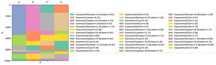
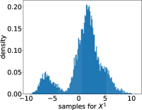
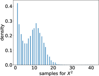
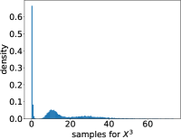
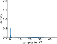
Figure 6: Synthetic data generation. (Top) An example of a partitioning for a synthetic dataset of $N=10000$ samples and $D=4$ features, where samples have been re-ordered to have contiguous partitions for the sake of visualization. Each partition is associated with a parametric likelihood model labeled by a color, instantiated with a set of parameters randomly drawn according to a sensible prior (see Appendix B). (Bottom) Histogram visualizations for the marginals of the $4$ features generated.

Appendix C C. Synthetic data experiments

C1. Synthetic data generation

Here we describe in detail the process we adopted for generating the 90 datasets employed in our controlled experiments. As stated in the main article, we consider an increasing number of samples $N\in\{2000,5000,10000\}$ and features $D\in\{4,8,16\}$ and for each combination of the two we generate 10 independent datasets. Later on, we split them into training, validation and test partitions (70%, 10%, 20% splits).

We generate each dataset by mimicing the structure learning process of an SPN. Please note that in such a way we are encompassing highly expressive and complex joint distributions that might have generated the data (while retaining control over their statistical dependencies, types and likelihood models. Indeed, SPNs have been demonstrated to capture linear [22] and highly non-linear correlations [23, 35] in the data, being also able to model constrained random vectors, as ones drawn from the simplex (see. [23]).

Each dataset is generated in the following way: For every feature, we fix a randomly selected type among real, positive, discrete numerical or nominal. To randomly create a ground truth generative model, i.e., an SPN—denoted as $\mathcal{S}^{\prime}$—we simulate a stochastic guillotine partitioning of a fictitious $N\times D$ data matrix. Specifically, we follow a LearnSPN-like [14, 34] structure learning scheme in which columns and rows of this matrix are clustered together, in this case in a random fashion.

At each iteration of the algorithm, it decides to try to split the columns or rows proportionally to a probability $\theta_{\mathsf{split}}=0.8$. For a tentative column split, the likelihood of a column to be assigned to one of two clusters is drawn from a $\mathsf{Beta}(a=4,b=5)$. In case all columns are assigned to a single cluster, no column split is performed and the process moves to the next iteration. Concerning row splits, on the other hand, each row is randomly assigned to one of two clusters with a probability drawn from $\mathsf{Beta}(a=4,b=5)$. We alternate these splitting processes until we reach a matrix partition with less than 10% of N number of rows. We assign these final partitions to univariate leave nodes in the spn. For each leaf node, we then randomly select a univariate parametric distribution valid for the type associated with the feature $d$, as listed in the previous Section.

An example of a synthetically generated dataset for $N=10000$ samples and $D=4$ features, and its random partitioning, is shown in Fig. 6. There, samples have been ordered in the data matrix (after performing bi-clustering) to enhance the visualization of contiguous partitions.

We employ the following priors to draw the corresponding parameters for each distribution: For Gaussian distributions we employ a $\mathsf{Normal-Inverse-Gamma}(\mu=0,V=30,a=10,b=10)$ for the mean and variance, we draw the shape parameter of the Gamma distributions from a $\mathsf{Uniform}(5,25)$ involved and their scale parameters from a $\mathsf{Gamma}(a=10,b=10)$ prior, while for Exponential distributions we randomly select the rate from a $\mathsf{Gamma}(a=20,b=5)$. For the discrete data, we draw the number of categories of a Categorical from a discrete $\mathsf{Uniform}(5,15)$. We then draw the corresponding probabilities from an equally sized and symmetric $\mathsf{Dirichlet}(\alpha=10)$; the mean parameter of Poissons is drawn from a $\mathsf{Gamma}(a=100,b=10)$.

C2. ABDA inference

We perform inference on ABDA for each synthetic dataset. We learn the LV structure by letting the RDC independence threshold parameter in $\{0.1,0.3,0.5\}$ while fixing to $10\%$ of $N$ the minimum number of samples to continue the partitioning process during SPN structure learning. We select then the best model w.r.t. the log-likelihood scored on a validation set. Then we run the Gibbs sampler for 3000 iterations discarding the first 2000 samples for burn-in.

For the log-likelihoods in Fig 2a, we estimate them as the mean log-likelihood computed by ABDA over the test samples and averaged across the last 1000 samples of the Gibbs chain.

For recovering the global weights measuring uncertainty over the likelihood models (or statistical data types), we average over the predicted arrays belonging to the last 1000 samples of Gibbs and perform the cosine similarity between these vector and the ground truth one.

For the hard predictions, as shown in the confusion matrixes in Fig.2, we select, from each vector, the likelihood model (or statistical data type) scoring the highest weight in the weight vector.

Appendix D D. Real-world datasets

D1. Density estimation and imputation datasets.

For our experiments we use some real-world datasets from the UCI[11] repository. The number of instances and features are what we used for the models after preprocessing. We took the datasets as available from [23] and [32] and put them in the same tabular formalism where we labeled each feature to be either continuous or discrete. We removed binary features from them and we either randomly selected a certain percentage of missing values for the transductive case or we randomly split them into train, validation and test sets for the inductive case (see main text).

Abalone is a dataset of abalone in Tasmania that includes different physical measurements. It contains 4177 instances, 9 features and no missing values. Adult is a "Census Income" dataset used to predict low or high income, it contains 32561 instances and 13 features. Australia contains information about credit card applications in Australia, with 690 and 10 features. Autism has data about the autistic spectrum disorder screening in adults. It contains 3521 instances and 25 features. Breast describes 10 attributes about 681 instances of two types of breast cancer. Chess is a chess endgame database, with 28056 and 7 features. Crx is a dataset of credit card applications, with 651 instances and 11 attributes. Dermatology provides 366 instances and 34 about the Eryhemato-Squamous dermatological disease. Diabetes is a dataset of diabetes patient records, with 768 instances and 8 features. German is a classification dataset of people described by a set of attributes as good or bad credit risks. It has 1000 instances and 17 attributes. Student is a dataset of student performance in secondary education. With 395 instances and 20 features. Wine is a dataset about wine quality based on physicochemical tests. It contains 6497 instances, with 12 features.

D2. Outlier detection datasets.

The datasets used for anomaly detection come from [17]. Thyroid is a dataset of thyroid diseases provided by the Garavan Institute of Sydney, Australia. It contains 6916 instances, 21 features, and 250 outliers. Letter contains classification data for 26 capital letters of the English alphabet. It contains 1600 instances, 32 features, and 100 outliers. Pen-* are datasets about pen-based handwritten digit recognition. Pen-global contains 809 instances, 16 features, and 90 outliers. Pen-local contains 6724, 16 features, and 10 outliers. Satellite is a dataset that contains multi-spectral values of pixels in 3x3 neighborhoods in a satellite image and a label for the central pixel. It contains 5100 instances, 36 features, and 75 outliers. Shuttle is a dataset about the space shuttle with 46464 instances, 9 features and 878 outliers. Speech is a speech recognition dataset with 3686 instances, 400 features and 61 outliers.

Appendix E E. Missing value estimation

E1. ABDA can efficiently marginalize over missing values during inference

In order to be able to deal with missing values at inference time, we first need to provide ABDA with a LV structure that has been induced from the non-missing data entries only. Secondly, we need to marginalize over these entries while performing Gibbs sampling. This can be done efficiently by exploiting SPNs’ ability to decompose marginal queries into simpler marginalizations at the leaf distributions [7, 25]. When updating the posterior parameters for the leaf likelihood models, we keep track of counts belonging only to non-missing entries.

To this end, we adapted the likelihood-agnostic structure learning introduced by MSPNs [23]. In a nutshell, in presence of missing entries in the training samples, these are not contributing to the evaluation of the RDC both for the partitioning along the rows of the data matrix (clustering), and for the partitioning along RVs or features (group independence seeking). Specifically, while transforming the data matrix through the copula transformation (for details, refer to [23]) we do not let missing entries contribute to the estimation of the empirical cumulative distribution. We reserve the same treatment for MSPNs as well.

E2. ABDA can estimate missing values efficiently

We assume each sample $\mathbf{x}_{n}$ to be in the form $\mathbf{x}_{n}=(\mathbf{x}_{n}^{o},\mathbf{x}_{n}^{m})$, where $\mathbf{x}_{n}^{o}$ comprises observed values and $\mathbf{x}^{m}_{n}$ missing ones.

To evaluate the effectiveness of a generative model $\mathcal{M}$ in estimating missing values, we employ the probability of seeing the true missing entries $\bar{\mathbf{x}}_{n}^{m}$, i.e., $p_{\mathcal{M}}(\bar{\mathbf{x}}_{n}^{m})$, as a standard approach indicating the ability of $\mathcal{M}$ of selecting the true value for a RV [32]. This operation requires marginalizing over all observed values $\mathbf{x}_{n}^{o}$, which can be done efficiently with SPN-based models [7, 25].

To impute missing values, on the other hand, we resolve to compute the the most probable explanation (MPE) [8] for the corresponding RVs, that is:

$$\tilde{\mathbf{x}}_{n}^{m}=\operatorname{\arg\max}_{\mathbf{x}_{n}^{m}}p_{\mathcal{M}}(\mathbf{x}_{n}^{m}|\mathbf{x}_{n}^{o})=\operatorname{\arg\max}_{\mathbf{x}_{n}^{m}}p_{\mathcal{M}}(\mathbf{x}_{n}^{m},\mathbf{x}_{n}^{o})$$

Note that this task is performed by factorization-based models like ISLV efficiently, since each RVs appearing in $\mathbf{x}^{m}_{n}$ is imputed independently from others. Conversely, ABDA and MSPNs can leverage all other RVs while performing imputation. The price to pay for this is that, for general SPNs, exact MPE imputation is NP-Hard [25, 5]. Nevertheless, reasonably accurate approximations to this tasks exist and allow to evaluate an SPN structure in linear time [7, 3]. In brief, they employ a bottom-up propagation step for observing $\mathbf{x}_{n}^{o}$, at first, while performing a Viterbi-like decoding top-down traversal of the SPN structure to retrieve the maximally likely states for the RVs in $\mathbf{x}^{m}_{n}$. Please refer to [25] for more details.

E3. Missing value estimation experiments

For our missing value estimation experiments in the transductive scenarios we monitor both the mean log-likelihood for the missing data entries in a run and the normalized root mean squared error (NRMSE) w.r.t. the imputation provided by each model (please refer to the previous Section for how to compute them in ABDA).

Figure 7 reports the feature-wise plots for the above mentioned metrics. As a general trend, one can see how ISLV performs less well than ABDA and MSPNs and how the difference between these two is often significant only on a small subset of the modeled features. Generally, it seems that ABDA has the advantage of modeling continuous RVs, confirming that the performing discretization as MSPNs do is potentially a problem. However, note also that in such cases, MSPNs log-likelihood values might be inflated by their adoption of piecewise polynomial approximations as likelihood models. Indeed, since they are fitted on the small range of values available during learning, their density is renormalized to integrate to 1. On the other hand, since the likelihood distributions used in ABDA generally have infinite tails, their mass is not concentrated only on that observed range.

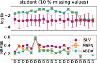
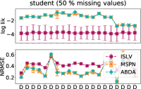
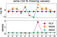
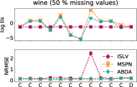
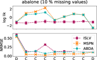
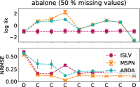
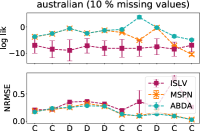
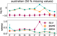
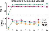
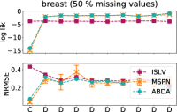
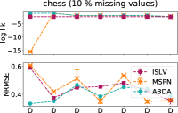
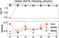
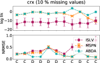
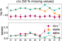
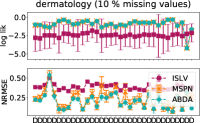
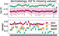
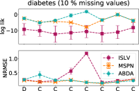
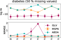
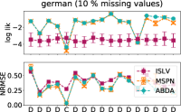
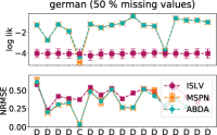
Figure 7: Performance (test log-likelihood, normalized RMSE feature-wise) on real datasets.

Appendix F F. Anomaly robustness and detection

F1. ABDA is robust to corrupted data and outliers

During inference, ABDA will tend to assign anomalous samples into low-weighted mixture components, i.e., sub-networks of the underlying SPN or leaf likelihood models. If more that one anomalous sample is relegated to the same partition, they will form a micro-cluster [4].

At test time, ABDA would assign low probability to outliers or novel samples. The (log-)likelihood of the whole joint distribution can be employed as a score for inliers [30, 4] and by proper thresholding, one can have a decision rule to detect anomalies.

This process can be repeated at each node in the underlying SPN structure, thus enabling ABDA to perform hierarchical anomaly detection to decide whether a sample—or just a subset of features in a sample (i.e., contextual outliers [4])—is anomalous with respect to the distribution induced at that node.

As a qualitative example, Figure 8 illustrates how ABDA partitioned the Shuttle data, correctly relegating most of the outliers into micro-clusters. Those not associated to a single micro-cluster are still belonging to the tail of the distribution modeling the time feature (x-axis).

Figure 8: ABDA separates outliers (pink ‘O’) from inliers (green ‘I’) via hierarchical partitioning on Shuttle data. Each ellipse represents a partition induced by the underlying SPN w.r.t. the first two features ($X^{0}$ and $X^{1}$) of the shuttle data. The thickness of the ellipses is inversely proportional to the number of samples in the corresponding partition, therefore it also indicates the depth of the partition—finer lines for finer grain clusters.

F2. Unsupervised outlier detection

We quantitatively evaluate how ABDA is able to perform unsupervised pointwise anomaly detection [4], that is detect outliers available at training time, without having access to their label.

We follow the experimental setting of [17], in which a set of UCI binary classification datasets have been processed to include all samples from one class (inliers) and a small percentage of dissimilar samples drawn from the other class (outliers). Please refer to [17] for detailed dataset statistics.

Once trained on these datasets, all models involved are required to output a score for each training sample, the higher the most confident the model is about the sample being an outlier. For ABDA, MSPN and ISLV we employ the sample negative log-likelihood as the outlier score.

As competitors we include one-class support vector machines (oSVM) [30], the local outlier factor (LOF) [2] and the histogram-based outlier score (HBOS) [16]. Accuracy performances for all models are measured in terms of the area under the receiving operating curve (AUC ROC) computed w.r.t. to the outlier scores.

We follow [17], and instead of picking one single model out of a grid search to optimize its hyperparameters, we average over all AUC scores from the cross validated models. We emply an RBF kernel ($\gamma=0.1$) for oSVMs, varying $\nu\in\{0.2,0.4,0.6,0.8\}$. For LOF, we run it by evaluating a number of nearest neighbors $k\in\{20,30,40,50\}$. For HBOS, instead, we explored these configurations with the Laplacian smoothing factor $\alpha\in\{0.1,0.2,0.5\}$ and number of bins in $\{10,20,30\}$. For ABDA and MSPNs we set the minimum number of instances $m$ to $5\%$ of the number of instances and explored the RDC coefficient $\rho\in\{0.1,0.3,0.5\}$. For ISLV, we run it several times for $k\in\{\left\lfloor\frac{D}{3}\right\rfloor,\left\lfloor\frac{D}{2}\right\rfloor,\left\lfloor\frac{2D}{3}\right\rfloor\}$.

Table 4: Unsupervised anomaly detection with ABDA. Mean and standard deviation (small) AUC ROC scores for all models and datasets.

	oSVM	LOF	HBOS	ABDA	MSPN	ISLV
Aloi	51.71	74.19	52.86	47.20	51.86	-
	$\scriptstyle\scriptstyle\pm 0.02$	$\scriptstyle\scriptstyle\pm 0.70$	$\scriptstyle\scriptstyle\pm 0.53$	$\scriptstyle\scriptstyle\pm 0.02$	$\scriptstyle\scriptstyle\pm 1.04$
Thyroid	46.18	62.38	62.77	84.88	77.74	-
	$\scriptstyle\scriptstyle\pm 0.39$	$\scriptstyle\scriptstyle\pm 1.04$	$\scriptstyle\scriptstyle\pm 3.69$	$\scriptstyle\scriptstyle\pm 0.96$	$\scriptstyle\scriptstyle\pm 0.33$
Breast	45.77	98.06	94.47	98.36	92.29	82.82
	$\scriptstyle\scriptstyle\pm 11.12$	$\scriptstyle\scriptstyle\pm 0.70$	$\scriptstyle\scriptstyle\pm 0.79$	$\scriptstyle\scriptstyle\pm 0.07$	$\scriptstyle\scriptstyle\pm 0.99$	$\scriptstyle\scriptstyle\pm 1.31$
Letter	63.38	86.55	60.47	70.36	68.61	61.98
	$\scriptstyle\scriptstyle\pm 17.60$	$\scriptstyle\scriptstyle\pm 2.23$	$\scriptstyle\scriptstyle\pm 1.80$	$\scriptstyle\scriptstyle\pm 0.01$	$\scriptstyle\scriptstyle\pm 0.23$	$\scriptstyle\scriptstyle\pm 0.44$
Kdd00	53.40	46.39	87.59	99.79	70.17	-
	$\scriptstyle\scriptstyle\pm 3.63$	$\scriptstyle\scriptstyle\pm 1.95$	$\scriptstyle\scriptstyle\pm 4.70$	$\scriptstyle\scriptstyle\pm 0.10$	$\scriptstyle\scriptstyle\pm 15.97$
Pen-global	46.86	87.25	71.93	89.87	75.93	75.54
	$\scriptstyle\scriptstyle\pm 1.02$	$\scriptstyle\scriptstyle\pm 1.94$	$\scriptstyle\scriptstyle\pm 1.68$	$\scriptstyle\scriptstyle\pm 2.87$	$\scriptstyle\scriptstyle\pm 0.14$	$\scriptstyle\scriptstyle\pm 5.40$
Pen-local	44.11	98.72	64.30	90.86	79.25	65.52
	$\scriptstyle\scriptstyle\pm 6.07$	$\scriptstyle\scriptstyle\pm 0.20$	$\scriptstyle\scriptstyle\pm 2.70$	$\scriptstyle\scriptstyle\pm 0.79$	$\scriptstyle\scriptstyle\pm 5.41$	$\scriptstyle\scriptstyle\pm 13.08$
Satellite	52.14	83.51	90.92	94.55	95.22	-
	$\scriptstyle\scriptstyle\pm 3.08$	$\scriptstyle\scriptstyle\pm 11.98$	$\scriptstyle\scriptstyle\pm 0.16$	$\scriptstyle\scriptstyle\pm 0.68$	$\scriptstyle\scriptstyle\pm 0.45$
Shuttle	89.37	66.29	98.47	78.61	94.96	-
	$\scriptstyle\scriptstyle\pm 5.13$	$\scriptstyle\scriptstyle\pm 1.69$	$\scriptstyle\scriptstyle\pm 0.24$	$\scriptstyle\scriptstyle\pm 0.02$	$\scriptstyle\scriptstyle\pm 2.13$
Speech	45.61	49.37	47.47	46.96	48.24	-
	$\scriptstyle\scriptstyle\pm 3.64$	$\scriptstyle\scriptstyle\pm 0.87$	$\scriptstyle\scriptstyle\pm 0.10$	$\scriptstyle\scriptstyle\pm 0.01$	$\scriptstyle\scriptstyle\pm 0.67$

Mean and average AUC scores are reported in Table 4. On the Thyroid dataset we were not able to run ISLV, while on the datasets where there is no value in Table 4 it either did not converge in 72hrs or in 1000 iterates. Otherwise, as for ABDA, we report the average AUC ROC w.r.t. the 100 last Gibbs samples after a burn-in of 3000 iterations. For KDD99, we observed ABDA converging in 1000 iterates (burn-in) and within the 72hrs limit.

It is clearly visible from Table 4 how ABDA can perform as good as, or even better in most cases than standard outlier detection models. Moreover, this unsupervised task demonstrates how ABDA is indeed more resilient to outliers and corrupt data w.r.t. MSPNs. Indeed, while the greedy structure learning procedure adopted by both MSPNs and ABDA can get fooled by some outliers, grouping them to inliers in the same partition, Bayesian inference in ABDA might be able to re-assign them to low-probability partitions.

Appendix G G. Exploratory pattern extraction

Here we discuss how to employ ABDA to unsupervisedly extract patterns among RVs—implying dependency among them—in a similar fashion to what Association Rule Mining (ARM) does [1]. The aim is, on the one hand, to automatize the way such patterns can be extracted, filtered and presented (as a ranking) to the user, and on the other hand, to extract a small set able to explain to the user—in a more interpretable way—what correlations ABDA has captured.

In ARM, given some data over discrete (generally assumed to be binary for simplicity) RVs $\mathbf{X}=\{X^{1},\dots,X^{D}\}$ one is interested in finding a set of association rules $\{\mathcal{R}_{i}\}$ where each rule $\mathcal{R}:\mathcal{A}\rightarrow\mathcal{C}$ is composed by an antecedent, $\mathcal{A}=P_{1}\wedge P_{2},\ldots,P_{a}$, and consequent, $\mathcal{C}=P_{a+1}\wedge P_{a+2},\ldots,P_{a+s}$, part, both of which are conjunctions of patterns, i.e. assignments to some RVs in $\mathbf{X}$. For instance one rule might state:

$$P_{1}:X^{1}=0\wedge P_{2}:X^{3}=1\rightarrow P_{3}:X^{2}=1$$

. which would state that whenever the antecedent is observed, i.e., $P_{1}$ and $P_{2}$ are satisfied, it is likely to observe $X^{2}$ set to value 1.

To quantify the “importance” of a rule—thus having a quantitative way to filter and rank rules— one computes for a rule $\mathcal{R}$ measures like its support and confidence. The former being defined as:

$$supp(\mathcal{R}:\mathcal{A}\rightarrow\mathcal{C})=\frac{\#\{P_{1},\ldots,P_{a},P_{a+1},\ldots,P_{r+s}\}}{N}$$

where the numerator indicates the number of samples for which the patterns $P_{1},\ldots,P_{a+s}$ are jointly satisfied and $N$ is the number of samples in the data. Confidence of a rule, instead is the ratio of its support and that of the antecedent:

$$conf(\mathcal{R}:\mathcal{A}\rightarrow\mathcal{C})=\frac{supp(\mathcal{A},\mathcal{C})}{supp(\mathcal{A})}=\frac{\#\{P_{1},\ldots,P_{a+s}\}}{\#\{P_{1},\ldots,P_{a}\}}$$

G1. Probabilistic patterns in ABDA

Clearly, the notion of support is the maximum likelihood estimation for the joint probability of its patterns

$$p(P_{1}\wedge\ldots\wedge P_{a}\wedge P_{a+1}\wedge\ldots\wedge P_{a+s})$$

Analogously, the confidence of a rule $\mathcal{R}$ is estimator for the conditional probability

$$p(P_{a+1}\wedge\ldots\wedge P_{a+s}|P_{1}\wedge\ldots\wedge P_{a})$$

.

By properly defining what a pattern is in ABDA, we might directly compute the above probabilities efficiently, by exploiting marginalization over the SPN structure of ABDA. We also have to take into consideration how to deal with continuous RVs natively, since the classical formulation of ARM patterns would require binarization.

We define an interval pattern over RV $X^{i}$ as the event $P:\pi_{low}^{i}\leq X^{i}<\pi_{high}^{i}$ where $\pi_{low}^{i}<\pi_{high}^{i}$ are two valid values from the domain of $X^{i}$. The probability of a single pattern is therefore:

$$p(P:\pi_{low}^{i}\leq X^{i}<\pi_{high}^{i})=\int_{\pi_{low}^{i}}^{\pi_{high}^{i}}f(X^{i})dX^{i}$$

where $f$ is the density function of $X^{i}$.

Consider now an dependency rule of the form $P_{1},\ldots P_{a}\rightarrow P_{a+1},\ldots,P_{a+s}$, its support can then be computed as multivariate integral over $P_{1}\ldots P_{a+s}$

$$\int_{\pi_{low}^{1}}^{\pi_{high}^{1}}\ldots\int_{\pi_{low}^{a+s}}^{\pi_{high}^{a+s}}f(\mathbf{X})dX^{1}\ldots X^{a+s}$$

If the joint density $f$ decomposes as an SPN structure, solving the above integral would require resolving univariate integrals at the leaves—which is doable assuming tractable univariate distributions there as we do in ABDA— and propagate the computed probabilities upwards.

By doing so we have a way to exploit the SPN structure in ABDA to efficiently compute the support of a rule—a collection of dependency pattern—here extended to continuous RVs. Therefore we can rank rules by computing their support. How to extract rules in a (semi-)automatic way?

G2. Automatic pattern mining in ABDA

The most straightforward approach to extract patterns and rules via ABDA would mimic Apriori, the stereotypical ARM algorithm. In a nutshell, first patterns of length 1 are mined (i.e., involving a single RV), the collection of patterns are combined by enumeration while at the same time filtering out patterns whose support is less than a user-specified threshold $\rho$ [1].

The main issue would be how to determine the atomic patterns in the form $P:\pi_{low}^{i}\leq X^{i}<\pi_{high}^{i}$, since we $X^{i}$ can also be continuous, and hence we can possibly find an infinite number of intervals $[\pi_{low}^{i},\pi_{high}^{i})$ from its domain. The solution comes from ABDA having already applied this partitioning during inference. Indeed, SPN leaves in ABDA already describe tractable distributions concentrated on a portion of the whole domain for a feature. Given a user defined percentile threshold $\lambda\in[0,1]$, we can determine the interval containing $\lambda$ percentage of the probability mass of density $f(X^{i})$. For instance, for $\lambda=90\%$, we might easily find $[\pi_{low}^{i},\pi_{high}^{i})$ as the the $5\%$ and $95\%$percentiles of $f(X^{i})$.

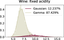
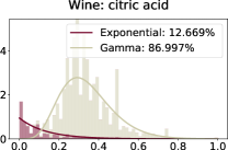
Figure 9: Data exploration on Wine data. Density estimation provided by ABDA on the Wine quality dataset. ABDA identifies the two modalities in the data induced by red and white wine over three different features.

G3. Wine data

As a concrete example, see Figure 9, depicting two marginal distributions as learned by ABDA for two features of the Wine dataset, $X^{1}=\mathsf{FixAcid}$ and $X^{2}=\mathsf{CitAcid}$. One might extract the following four patterns from them by fixing a threshold of $80\%$ of probability:

$$P_{1}:5.8\leq{\color[rgb]{0.80078125,0.79296875,0.6640625}\mathsf{FixAcid}}<8.1,\quad{\color[rgb]{0.80078125,0.79296875,0.6640625}\mathsf{FixAcid}}\sim\mathcal{N}$$

$$P_{2}:0.2\leq{\color[rgb]{0.80078125,0.79296875,0.6640625}\mathsf{CitAcid}}<0.5,\quad{\color[rgb]{0.80078125,0.79296875,0.6640625}\mathsf{CitAcid}}\sim Gamma$$

$$P_{3}:7.1\leq{\color[rgb]{0.46484375,0.0390625,0.17578125}\mathsf{FixAcid}}<12.0,\quad{\color[rgb]{0.46484375,0.0390625,0.17578125}\mathsf{FixAcid}}\sim Gamma$$

$$P_{4}:0.0\leq{\color[rgb]{0.46484375,0.0390625,0.17578125}\mathsf{CitAcid}}<0.3,\quad{\color[rgb]{0.46484375,0.0390625,0.17578125}\mathsf{CitAcid}}\sim Exp$$

After these atomic patterns have been extracted from leaves, one can first determine their support according to the whole SPN $\mathcal{S}$ Then, conjunctions of patterns may be mechanically combined as in Apriori, their support computed and filtered out if it is lower than the user-defined threshold $\rho$.

Back to the Wine features in Figure 9, one could compose the following composite pattern via conjunctions, by noting that the extracted patterns are belonging to product node children and thus referring to samples belonging the same partition (same color across histograms):

$$P_{1}:5.2\leq{\color[rgb]{0.80078125,0.79296875,0.6640625}\mathsf{FixAcid}}<8.1\wedge P_{2}:0.2\leq{\color[rgb]{0.80078125,0.79296875,0.6640625}\mathsf{CitAcid}}<0.5$$

$$P_{3}:7.1\leq{\color[rgb]{0.46484375,0.0390625,0.17578125}\mathsf{FixAcid}}<12.0\wedge P_{4}:0.0\leq{\color[rgb]{0.46484375,0.0390625,0.17578125}\mathsf{CitAcid}}<0.3$$

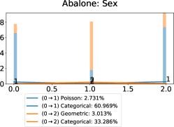
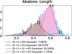
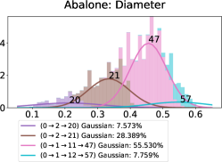
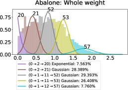
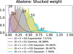
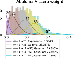
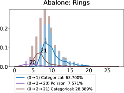
Figure 10: Data exploration on Abalone. Density estimation provided by ABDA on the Abalone UCI dataset, showing the extracted correlation patterns among sub-populations across different features like shell and viscera weights, sex and shell diameter and length. Equally colored densities model samples assigned by ABDA to the same sub-population (partition), while their numerical label indicates the position of such partition in the hierarchical decomposition discovered (paths are represented in parenthesis as sequences of labeled partitions, starting from the initial partition, representing the root of the hierarchy.)

G4. Abalone data

For a more complex example, we employ ABDA on the Abalone dataset (see Appendix D). The dataset contains physical measurements (features) over abalone samples, namely: the Sex of the specimen (’male’, ’female’ or ’infant’), its Length, Diameter, Height, Whole weight, Shucked Weight and Viscera Weight, its Shell Weight and the number of rings in it.

We employ ABDA on it by running it for 5000 iterates, stopping the SPN LV structure learning until 10% of the data was reached and employing $0.7$ as the RDC independence threshold.

Figure 10 shows the marginal distributions for all features upon which the densities as fit by ABDA. Each density is colored by a unique color—shared across all features—indicating the partition $\mathcal{K}$ induced by the SPN $\mathcal{S}$. Each of such partitions is also labeled with an integer, which serves the purpose to indicate the path—appearing in each legend entry—inside $\mathcal{S}$ leading from the top partition (numbered as 0, indicating the whole data matrix) to the finer grained one. For instance, the path $0\rightarrow 2\rightarrow 20$ appearing in the legend of the Length attribute, and associated to the purple partition numbered 20, indicates that such a partition is contained in the partition number 2 which in turn belongs to the initial partition.

By starting from the Sex feature, one can see that two partitions are discovered (1 and 2) in which the first mostly represents samples belonging to the first and last mode of the categorical features, indicating ’male’ and ’infant’ abalone samples, while the second comprises mostly ’female’ individuals. From these initial conditioning on the sex, all other feature correlations are characterized.

For instance, the green partition (11) is a sub-partition of the ’Male’ clustering, and shows a cross correlation across the Height feature and the Weight one, as one would expect. Additionally, the green partition itself later on splits into two sub-population, the gray (52) and yellow (53) representing correlations among the Shucked and Viscera weights, indicating a mode in the abalone population for specific ranges of these features.

By looking at all partitions and at each density belonging to them, one can build in a mechanical way (composite) patterns and rank them by their support. For this analysis of the Abalone data, these are the top 5 patterns that the ABDA automatically extracts:

$$\mathcal{P}_{1}:\quad 0.088 \leq{\color[rgb]{0.171875,0.62890625,0.171875}\mathsf{Height}}<0.224\quad\wedge\quad 0.158\leq{\color[rgb]{0.171875,0.62890625,0.171875}\mathsf{ShellWeight}}<0.425\quad(supp(\mathcal{P}_{1})=0.507)$$

$$\mathcal{P}_{2}:\quad 0.483 \leq{\color[rgb]{0.890625,0.46484375,0.76171875}\mathsf{Length}}<0.684\quad\wedge\quad 0.364\leq{\color[rgb]{0.890625,0.46484375,0.76171875}\mathsf{Diameter}}<0.547\quad(supp(\mathcal{P}_{2})=0.489)$$

$$\mathcal{P}_{3}:\quad 0.596 \leq{\color[rgb]{0.49609375,0.49609375,0.49609375}\mathsf{WholeWeight}}<1.040\quad\wedge\quad 0.205\leq{\color[rgb]{0.49609375,0.49609375,0.49609375}\mathsf{ShuckedWeight}}<0.491\quad\wedge$$

$$0.076 \leq{\color[rgb]{0.49609375,0.49609375,0.49609375}\mathsf{VisceraWeight}}<0.281\quad(supp(\mathcal{P}_{3})=0.223)$$

$$\mathcal{P}_{4}:\quad 0.596 \leq{\color[rgb]{0.73828125,0.7421875,0.1328125}\mathsf{WholeWeight}}<1.040\quad\wedge\quad 0.205\leq{\color[rgb]{0.73828125,0.7421875,0.1328125}\mathsf{ShuckedWeight}}<0.491\quad\wedge$$

$$0.076 \leq{\color[rgb]{0.73828125,0.7421875,0.1328125}\mathsf{VisceraWeight}}<0.281\quad(supp(\mathcal{P}_{4})=0.202)$$

$$\mathcal{P}_{5}:\quad 0.313 \leq{\color[rgb]{0.55078125,0.3359375,0.29296875}\mathsf{Length}}<0.554\quad\wedge\quad 0.230\leq{\color[rgb]{0.55078125,0.3359375,0.29296875}\mathsf{Diameter}}<0.438\quad\wedge$$

$$\quad 0.023 \leq{\color[rgb]{0.55078125,0.3359375,0.29296875}\mathsf{Height}}<0.197\quad\wedge\quad 0.165\leq{\color[rgb]{0.55078125,0.3359375,0.29296875}\mathsf{WholeWeight}}<0.639\quad\wedge$$

$$0.037 \leq{\color[rgb]{0.55078125,0.3359375,0.29296875}\mathsf{ShuckedWeight}}<0.408\quad\wedge\quad 0.019\leq{\color[rgb]{0.55078125,0.3359375,0.29296875}\mathsf{VisceraWeight}}<0.192\quad\wedge$$

$$0.027 \leq{\color[rgb]{0.55078125,0.3359375,0.29296875}\mathsf{ShellWeight}}<0.27\quad\wedge\quad 5\leq{\color[rgb]{0.55078125,0.3359375,0.29296875}\mathsf{Rings}}<13\quad(supp(\mathcal{P}_{5})=0.111)$$

Appendix H H. ABDA vs MSPN: accuracy and robustness

In our experimental section, we selected diverse datasets—w.r.t. size and feature heterogeneity—from both the ISLV and MSPN original papers with the aim to have a common, fair experimental setting. Moreover, we run for ABDA and MSPN a grid search in the same hyperparameter space, to block the effect of building the SPN LV hierarchy. Striving for automatic density analysis, such a grid search has been limited only to the independence test (RDC) threshold parameter, while original MSPNs were validated over more than five parameters.

For a more straightforward comparison in the original experimental setting of [23], we cross-validate ABDA also on one additional parameter, $m\in\{20\%,10\%,5\%\}$, the minimum number of samples in a partition (as a percentage over the whole number of samples) to stop the learning process to recursively further partition it. This parameter governs the degree of overparametrization of the learned LV structure.

Table 5 reports the average test log-likelihoods for the best ABDA model on the validation set, while MSPN results, considering unimodal isotonic regression applied to piecewise linear leaf distribution approximations, are directly taken from [23]. As one can see, ABDA provides competitive results to MSPNs even in this experimental setting, still requiring less parameter tuning. This is due to i) the likelihood mixtures in ABDA better generalizing than piecewise models—since their support is limited to samples seen during training and possibly infinite tails of a distribution are not natively captured—and ii) our Bayesian inference providing indeed robust models.

Table 5: Density estimation by ABDA vs MSPN over the original 14 datasets. Best average test log-likelihoods in bold.

	ABDA	MSPN		ABDA	MSPN
Anneal-U	-2.65	-38.31	Austr.	-17.70	-31.02
Auto	-70.62	-70.06	Bal-scale	-7.13	-7.30
Breast	-25.46	-24.04	Bre.-cancer	-9.61	-9.99
Cars	-35.04	-30.52	Cleve	-22.60	-25.44
Crx	-15.53	-31.72	Diabete	-17.48	-27.24
German	-32.10	-32.36	Ger.-org	-26.29	-27.29
Heart	-23.39	-25.90	Iris	-2.96	-2.84

To get a better understanding of how Bayesian inference in ABDA affects its robustness, we compare ABDA and MSPNs in an inductive scenario when we provide both with increasingly parametrized LV structures. More specifically, for both we explore deeper and deeper structures by letting the minimum sample percentage parameter $m$ vary in $\{5\%,1\%,0.5\%\}$, while we fix the RDC independence threshold to $0.5$. As one could expect, ABDA is at advantage since it performs an additional parameter learning step after the structure is provided. Nevertheless, it is worth measuring by how much more robust ABDA models are to an overparametrization than MSPNs and, at the same time, evaluate how much sparser the SPN structure in ABDA gets, that is, quantifying how “blindly” one user can run ABDA with limited or no possibility to cross-validate.

To this end, we measure the relative percentage of decreasing mean test log-likelihoods w.r.t. the mean test log-likelihood achieved by each model in the case in which $m=5\%$. Moreover, we measure the sparsity of a SPN structure in ABDA as the ratio between the number of relevant product nodes and leaf likelihood components over the number of all nodes and likelihood models. In this case, the relevancy of a node is measured by the fact that at least some samples have been associated to the corresponding node (or likelihood component) partition.

Table 6 reports these values for the 12 datasets involved in our density estimation and imputation experiments. Firstly, one can see that on the Chess and German datasets, growing a deeper SPN structure is not even possible, in general. However, for all other datasets, it is clear that MSPN accuracy tends to drop more quickly than ABDA’s, whose test predictions are not only more stable for different values of $m$ but sometimes even better. Lastly, the sparsity of the SPN structure in ABDA is indeed significantly increasing as $m$ becomes smaller.

Table 6: Robustness of MSPN and ABDA w.r.t. overparametrized structures, i.e. when the minimum percentage of samples ($m$) to split a partition is let vary up to $0.5\%$ Best relative test log-likelihoods improvement w.r.t. test log likelihoods for $m=5\%$ is reported in bold (in parenthesis). The last column reports the sparsity of ABDA structures ($s$) after inference, for each setting.

dataset	$m$	MSPN		ABDA		s
abalone	$5\%$	10.33		4.94		0.15
	$1\%$	10.16	($\mathbf{-1.68}\%$)	4.74	($-4.13\%$)	0.04
	$0.5\%$	9.59	($-7.15\%$)	5.00	($\mathbf{+1.30}\%$)	0.03
chess	$5\%$	-16.21		-12.54		0.66
	$1\%$	-16.21	($\mathbf{-0.00}\%$)	-12.54	($\mathbf{-0.00}\%$)	0.69
	$0.5\%$	-16.21	($\mathbf{-0.00}\%$)	-12.54	($-0.00\%$)	0.69
german	$5\%$	-31.85		-25.86		0.56
	$1\%$	-31.85	($\mathbf{-0.00}\%$)	-26.21	($-1.35\%$)	0.45
	$0.5\%$	-31.85	($\mathbf{-0.00}\%$)	-25.87	($\mathbf{-0.05}\%$)	0.59
student	$5\%$	-36.86		-28.93		0.25
	$1\%$	-44.86	($-21.70\%$)	-29.16	($\mathbf{-0.78}\%$)	0.09
	$0.5\%$	-49.95	($-35.49\%$)	-29.32	($\mathbf{-1.35}\%$)	0.05
wine	$5\%$	-0.10		-9.20		0.14
	$1\%$	-0.31	($-198.38\%$)	-8.43	($\mathbf{+8.37}\%$)	0.17
	$0.5\%$	-0.51	($-391.74\%$)	-8.73	($\mathbf{+5.05}\%$)	0.07
dermat.	$5\%$	-35.77		-24.96		0.36
	$1\%$	-46.82	($-30.91\%$)	-25.14	($\mathbf{-0.72}\%$)	0.20
	$0.5\%$	-57.42	($-60.54\%$)	-25.16	($\mathbf{-0.78}\%$)	0.14
anneal-U	$5\%$	-151.09		7.68		0.12
	$1\%$	-156.60	($\mathbf{-3.64}\%$)	3.80	($-50.53\%$)	0.14
	$0.5\%$	-166.26	($\mathbf{-10.04}\%$)	4.33	($-43.53\%$)	0.08
austral.	$5\%$	-37.67		-15.89		0.27
	$1\%$	-38.93	($-3.32\%$)	-16.27	($\mathbf{-2.38}\%$)	0.21
	$0.5\%$	-40.08	($-6.37\%$)	-16.36	($\mathbf{-2.98}\%$)	0.13
autism	$5\%$	-41.16		-27.69		0.23
	$1\%$	-42.30	($-2.78\%$)	-27.60	($\mathbf{+0.35}\%$)	0.12
	$0.5\%$	-42.54	($-3.34\%$)	-27.33	($\mathbf{+1.29}\%$)	0.10
breast	$5\%$	-33.42		-25.52		0.23
	$1\%$	-34.87	($-4.32\%$)	-26.01	($\mathbf{-1.89}\%$)	0.20
	$0.5\%$	-35.84	($-7.23\%$)	-25.64	($\mathbf{-0.46}\%$)	0.10
crx	$5\%$	-37.57		-12.86		0.45
	$1\%$	-38.79	($-3.26\%$)	-13.03	($\mathbf{-1.37}\%$)	0.18
	$0.5\%$	-39.39	($-4.87\%$)	-13.00	($\mathbf{-1.07}\%$)	0.14
diabetes	$5\%$	-31.55		-16.47		0.41
	$1\%$	-31.70	($\mathbf{-0.45}\%$)	-18.96	($-15.07\%$)	0.31
	$0.5\%$	-31.65	($\mathbf{-0.31}\%$)	-17.91	($-8.75\%$)	0.27
adult	$5\%$	-74.98		-5.50		0.28
	$1\%$	-76.15	($-1.55\%$)	-5.37	($\mathbf{+2.50}\%$)	0.17
	$0.5\%$	-77.25	($-3.03\%$)	-5.36	($\mathbf{+2.62}\%$)	0.13

References

- [1] Rakesh Agrawal and Ramakrishnan Srikant. Fast algorithms for mining association rules. In Proceedings of VLDB, volume 1215, pages 487–499, 1994.
- [2] Markus M Breunig, Hans-Peter Kriegel, Raymond T Ng, and Jörg Sander. LOF: identifying density-based local outliers. In ACM sigmod record, volume 29, pages 93–104, 2000.
- [3] Hei Chan and Adnan Darwiche. On the robustness of most probable explanations. In Proceedings of the Twenty-Second Conference on Uncertainty in Artificial Intelligence, UAI’06, pages 63–71, Arlington, Virginia, United States, 2006. AUAI Press.
- [4] Varun Chandola, Arindam Banerjee, and Vipin Kumar. Anomaly detection: A survey. ACM Comput. Surv., 41(3):15:1–15:58, July 2009.
- [5] Arthur Choi and Adnan Darwiche. On relaxing determinism in arithmetic circuits. In Proceedings of ICML, pages 825–833, 2017.
- [6] Mary Kathryn Cowles and Bradley P Carlin. Markov chain monte carlo convergence diagnostics: a comparative review. Journal of the American Statistical Association, 91(434):883–904, 1996.
- [7] Adnan Darwiche. A differential approach to inference in Bayesian networks. Journal of the ACM (JACM), 50(3):280–305, 2003.
- [8] Adnan Darwiche. Modeling and Reasoning with Bayesian Networks. Cambridge, 2009.
- [9] Aaron Dennis and Dan Ventura. Learning the architecture of sum-product networks using clustering on variables. In Proceedings of NIPS, pages 2033–2041, 2012.
- [10] Aaron Dennis and Dan Ventura. Greedy Structure Search for Sum-product Networks. In IJCAI’15, pages 932–938. AAAI Press, 2015.
- [11] Dua Dheeru and Efi Karra Taniskidou. Uci machine learning repository. University of California, Irvine, School of Information and Computer Sciences, 2017.
- [12] David K. Duvenaud, James Robert Lloyd, Roger B. Grosse, Joshua B. Tenenbaum, and Zoubin Ghahramani. Structure discovery in nonparametric regression through compositional kernel search. In Proceedings of ICML, pages 1166–1174, 2013.
- [13] Robert Gens and Pedro Domingos. Discriminative learning of sum-product networks. In Proceedings of NIPS, pages 3239–3247, 2012.
- [14] Robert Gens and Pedro Domingos. Learning the structure of sum-product networks. In Proceedings of ICML, pages 873–880, 2013.
- [15] Zoubin Ghahramani and Matthew J Beal. Variational inference for Bayesian mixtures of factor analysers. In Proceedings of NIPS, pages 449–455, 2000.
- [16] Markus Goldstein and Andreas Dengel. Histogram-based outlier score (HBOS): A fast unsupervised anomaly detection algorithm. KI-2012, pages 59–63, 2012.
- [17] Markus Goldstein and Seiichi Uchida. A comparative evaluation of unsupervised anomaly detection algorithms for multivariate data. PloS one, 11(4), 2016.
- [18] I. Guyon, I. Chaabane, J. H. Escalante, and S. Escalera. A brief review of the chalearn automl challenge: Any-time any-dataset learning without human intervention. In ICML Workshop on AutoML, 2016.
- [19] James Robert Lloyd, David K. Duvenaud, Roger B. Grosse, Joshua B. Tenenbaum, and Zoubin Ghahramani. Automatic construction and natural-language description of nonparametric regression models. In AAAI, 2014.
- [20] David Lopez-Paz, Philipp Hennig, and Prof. Bernhard Schölkopf. The randomized dependence coefficient. In NIPS, 2013.
- [21] V. Mansinghka, P. Shafto, E. Jonas, C. Petschulat, M. Gasner, and J. B Tenenbaum. Crosscat: A fully bayesian nonparametric method for analyzing heterogeneous, high dimensional data. JMLR, 2016.
- [22] Alejandro Molina, Sriraam Natarajan, and Kristian Kersting. Poisson sum-product networks: A deep architecture for tractable multivariate poisson distributions. In AAAI, 2017.
- [23] Alejandro Molina, Antonio Vergari, Nicola Di Mauro, Sriraam Natarajan, Floriana Esposito, and Kristian Kersting. Mixed sum-product networks: A deep architecture for hybrid domains. In AAAI, 2018.
- [24] Kevin P. Murphy. Machine Learning: A Probabilistic Perspective. MIT Press, 2012.
- [25] Robert Peharz, Robert Gens, Franz Pernkopf, and Pedro Domingos. On the latent variable interpretation in sum-product networks. IEEE Transactions on Pattern Analysis and Machine Intelligence, 39(10):2030–2044, 2017.
- [26] Robert Peharz, Sebastian Tschiatschek, Franz Pernkopf, and Pedro Domingos. On theoretical properties of sum-product networks. AISTATS, 2015.
- [27] Hoifung Poon and Pedro Domingos. Sum-Product Networks: a New Deep Architecture. UAI 2011, 2011.
- [28] Andrzej Pronobis, Francesco Riccio, and Rajesh PN Rao. Deep spatial affordance hierarchy: Spatial knowledge representation for planning in large-scale environments. In ICAPS 2017 Workshop, 2017.
- [29] Amirmohammad Rooshenas and Daniel Lowd. Learning Sum-Product Networks with Direct and Indirect Variable Interactions. In ICML, 2014.
- [30] Bernhard Schölkopf, John C. Platt, John C. Shawe-Taylor, Alex J. Smola, and Robert C. Williamson. Estimating the support of a high-dimensional distribution. Neural Comput., 13(7):1443–1471, July 2001.
- [31] Martin Trapp, Tamas Madl, Robert Peharz, Franz Pernkopf, and Robert Trappl. Safe semi-supervised learning of sum-product networks. UAI, 2017.
- [32] I. Valera, M. F. Pradier, and Z. Ghahramani. General Latent Feature Models for Heterogeneous Datasets. ArXiv e-prints, June 2017.
- [33] Isabel Valera and Zoubin Ghahramani. Automatic discovery of the statistical types of variables in a dataset. In ICML, pages 3521–3529, 06–11 Aug 2017.
- [34] Antonio Vergari, Nicola Di Mauro, and Floriana Esposito. Simplifying, Regularizing and Strengthening Sum-Product Network Structure Learning. In ECML-PKDD 2015, 2015.
- [35] Antonio Vergari, Nicola Di Mauro, and Floriana Esposito. Visualizing and understanding sum-product networks. MLJ, 2018.
- [36] Antonio Vergari, Robert Peharz, Nicola Di Mauro, Alejandro Molina, Kristian Kersting, and Floriana Esposito. Sum-product autoencoding: Encoding and decoding representations using sum-product networks. In AAAI, 2018.
- [37] Han Zhao, Pascal Poupart, and Geoffrey J Gordon. A unified approach for learning the parameters of sum-product networks. In NIPS, pages 433–441. Curran Associates, Inc., 2016.