Parallel Whale Optimization Algorithm for Solving Constrained and Unconstrained Optimization Problems

Abstract

Recently the engineering optimization problems require large computational demands and long solution time even on high multi-processors computational devices. In this paper, an OpenMP inspired parallel version of the whale optimization algorithm (PWOA) to obtain enhanced computational throughput and global search capability is presented. It automatically detects the number of available processors and divides the workload among them to accomplish the effective utilization of the available resources. PWOA is applied on twenty unconstrained optimization functions on multiple dimensions and five constrained optimization engineering functions. The proposed parallelism PWOA algorithms performance is evaluated using parallel metrics such as speedup, efficiency. The comparison illustrates that the proposed PWOA algorithm has obtained the same results while exceeding the sequential version in performance. Furthermore, PWOA algorithm in the term of computational time and speed of parallel metric was achieved better results over the sequential processing compared to the standard WOA.

1 Introduction

Optimization algorithms are needed everywhere and became a major part of nearly all applications. For instance; problems in basic science, engineering, medical sciences, and data science with all its countless applications. Upon using any optimization algorithm to solve problems, there are specific steps to be followed. The first step is to determine the objective function (or functions) of the problem and whether they should be maximized or minimized. The second step is to select a group of constraints that control the problem if they exist. The third step, determine the problem variables and investigate whether they are continues or discrete variables and the range of these variables. Optimization algorithms are generally utilized to obtain either the optimal or nearly optimal solution to a given problem as the exact solution are impossible or hard to find. There are many optimization algorithms. Researchers are still providing new algorithms every day hoping to find closer solutions. Meta-heuristic swarm-based algorithms recently emerged as a promising direction. This type of algorithms has proved to be highly efficient in approaching to the optimal solutions.

Meta-heuristic algorithms [1] are divided into several categories. The first category is evolutionary algorithms, such as genetic algorithms (GA) [1], genetic programming (GP) [2], evolution strategy (ES) [3], probability-based incremental learning (PBIL) [4], and biogeography-based optimizer (BBO) [5]. The second category is physics-based methods, this type mimic the physical rules in the universe. Some algorithms of this type are central force optimization (CFO) [6], gravitational search (GLSA) [7], gravitational algorithm (GSA) [8], and charged search (CSS) [9]. The third category is human-based algorithms; this type depends on behavior of humans. This type contains some of the most popular algorithms like group search optimizer (GSO) [10], harmony search (HS) [11], and teaching-learning based optimization (TLBO) [12]. The last category comprised of swarm-based algorithms that simulate the social behavior of animals. Particle swarm optimization (PSO) is considered the most popular algorithm in this category and originally, is developed by Kennedy and Eberhart [13], [35]. Also, ant colony optimization [14], ant lion optimizer [15], dragonfly algorithm [16], moth-flame optimization algorithm [17], and finally whale optimization algorithm (WOA) [18] in which in this paper we will propose a parallelization WOA version.

WOA is one of promising swarm optimization algorithms. WOA simulates the behavior of the humpback whale. Hunting method is considered the most interesting characteristic for the humpback whales. Also, the bubble-net feeding method describes the foraging behavior [19]. Humpback whales are similar to hunt krill or fishes schools closed to the surface. Furthermore, the foraging behaviors are accomplished by creating distinctive bubbles over a circle (9-shape). However, the foraging behavior has investigated by [20]. Goldbogen et al. has captured 300 bubble-net nutrition of nine separate humpback whales utilizing tag sensors. the obtained results, two correlating maneuvers with bubble and named have been found called ‘upward-spirals’ and ‘double-loops’. Orderly former, humpback immersion dive around twelve m to down and the bubble in a circle is starting around the prey and in the end, it swims up toward the surface. The comprehensive information about the foraging behaviors is founded in [20]. Mathematically, the spiral bubble-net feeding behavior has been modeled in order to solve many optimization problems. The location of prey has determined by Humpback whales and encircle them. In advance, the optimal position is not known in the search space and the present best agent solution has been assumed by WOA is considered the target prey or near to the optimal. whereas the best solution is obtained, other search agents aim to update their positions according to the best one.

Recently, the use of multi-processor architectures for general-purpose, high-performance parallel computing has been attracting researchers’ interest more and more, especially after the arrival datasets are becoming increasingly large, many applications and problems have huge amounts of data to be processed. So, with a bottleneck problem is being faced in terms of hardware capabilities for the above-mentioned algorithms. Also, the execution time is therefore often the only direct objective quantitative parameter on which comparisons can be based. The objective of this study is to design an OpenMP inspired parallel processing from the basic WOA to maximize its competitive advantage as it will be more efficient in handling big datasets. The proposed parallel algorithm is tested against twenty unconstrained functions and five constrained engineering problems [21].

The structure of this paper is organized as follows; in Section 2 the basics and background are described. In Section 3, the pseudo code for the parallel whale optimization algorithms is presented. In Section 4 the experimental results are illustrated to evaluate the proposed PWOA algorithm’s performance. Finally, Section 5 draws the conclusions and future work.

2 Basics and Background

2.1 OpenMp

OpenMP is the most representative parallelization library of the SMP approach [22]. OpenMP is also referred to as “fork-join parallelism” because a thread forks when a parallel region starts and threads join when a parallel region ends [23]. OpenMP is composed of a set of directives [24], [25]. Therefore, it is easy to program for parallelization using OpenMP. Also, OpenMP is scalable. The parallelized code using OpenMP can be applied to a single processor and multiple processors with the same source code. The use of single or multiple cores in calculations is determined depending on whether the OpenMP compiler is activated or not. In addition, OpenMP is portable, therefore, when a code is parallelized using OpenMP on one platform, the parallelized code can be used on other platforms with the use of the OpenMP compiler option turned on. In general, OpenMP is efficient for code parallelization because it does not re- quire programming the entire code. Instead, it can be developed just by modifying parts of the code. Thus, it requires less time to parallelize a code, and yields excellent performance with little effort [26].

In the past, OpenMP had a limitation in the reduction of calculation time because the maximum number of core in the CPU was only four, six, or eight. However, the number of cores in CPU has increased dramatically as the relevant technology advances. Processors with dozens of core are now widely available. Currently, the interest in OpenMP is rising again because OpenMP is more convenient to program than MPI and requires only improvements to the original code rather than writing a new code. OpenMP has been successfully used to parallelize code. Recently, OpenMP was used to parallelize the finite element analysis program (FEAP) [27], and the authors compared the performance of the parallel code Warp3D and the parallelized FEAP code using OpenMP.

2.2 Whale Optimization Algorithm (WOA)

The mathematical model for WOA is illustrated in this section and for more detailed can found in [19]. The following Equations describes the behavior of WOA to achieve encircling prey, spiral bubble-net feeding, and prey search.

$$\overrightarrow{D}=|\overrightarrow{C}.\overrightarrow{X^{*}}(t)-\overrightarrow{X}(t)|$$ (1)

$$\overrightarrow{X}(t+1)=\overrightarrow{X^{*}}(t)-\overrightarrow{A}.\overrightarrow{D}$$ (2)

$$\overrightarrow{A}=2\overrightarrow{a}.\overrightarrow{r}-\overrightarrow{a}$$ (3)

$$\overrightarrow{C}=2.\overrightarrow{r}$$ (4)

$$\overrightarrow{X}(t+1)=\overrightarrow{D^{^{\prime}}}.e^{b1}.cos(2\pi l)+\overrightarrow{X^{*}}(t)$$ (5)

$$\overrightarrow{X}(t+1)=\left\{\begin{matrix}\overrightarrow{{{X}^{*}}}(t)-\overrightarrow{A.}\overrightarrow{D}\,\,\,\,if\,P\prec 0.5\\ \overrightarrow{{{D}^{{}^{\prime}}}}.{{e}^{b1}}.\cos(2\pi l)+\overrightarrow{{{X}^{*}}}(t)\,\,\,\,\,if\,P\geq 0.5\\ \end{matrix}\right.\,\$$ (6)

Where $\overrightarrow{D^{^{\prime}}}=\left|\overrightarrow{X^{*}}(t)-\overrightarrow{X}(t)\right|$

$$\overrightarrow{D}=\left|\overrightarrow{C.}\overrightarrow{{{X}_{rand}}}-\overrightarrow{X}(t)\right|\$$ (7)

$$\overrightarrow{X}(t+1)=\left|\overrightarrow{{{X}_{rand}}}-\overrightarrow{A}.\overrightarrow{D}\right|$$ (8)

Where $\,P\in[0,\,1],\,l\in[-1,\,1],\,b=1.$

2.3 Unconstrained Benchmark Functions

Twenty optimization unconstrained functions are presented in this section. These unconstrained problems is a classical benchmark functions and utilizing in the optimization literature [28], [29]. These unconstrained functions are described in Table 1 and 2 with the number of variable (N), variables ranges and the minimum value for each function.

Table 1: Unimodal unconstrained benchmark functions.

No.	Function	Range	N	Min (f)
f1	${\sideset{}{}{\sum}_{i=1}^{n}}z_{j}^{2}$	[-100,100]	30	0
f2	$\sum\limits_{j=1}^{n}{\left|{{Z}_{j}}\right|}+\prod\limits_{j=1}^{n}{\left|{{Z}_{j}}\right|}$	[-10,10]	30	0
f3	${\sideset{}{}{\sum}_{i=1}^{n}}(\sideset{}{}{\sum}_{j-1}^{i}Z_{j})^{2}$	[-100,100]	30	0
f4	$\underset{j}{max}\{\left|{{Z}_{j}}\right|,1\leq j\leq n\}$	[-100,100]	30	0
f5	${\sideset{}{}{\sum}_{j=1}^{n-1}}(100(Z_{j+1}-Z_{j}^{2})^{2}+(Z_{j}-1)^{2})$	[-30,30]	30	0
f6	${\sideset{}{}{\sum}_{j=1}^{n}}(Z_{j}+0.5)^{2}$	[-100,100]	30	0
f7	${\sideset{}{}{\sum}_{j=1}^{n}}jZ_{j}^{4}+rand[0,1)$	[-1.28,1.28]	30	0

Table 2: Multimodal unconstrained benchmark functions.

No.	Function	Range	N	Min (f)
f8	$\sum\nolimits_{j=1}^{n}{-{{Z}_{j}}}\sin(\sqrt{\left|{{Z}_{j}}\right|})$	[-500,500]	30	-418.98*5
f9	${\sideset{}{}{\sum}_{i=1}^{n}}[z_{j}^{2}-10cos(2\pi z_{j})+10]$	[-5.12,5.12]	30	0
f10	$-20\exp(-0.2\sqrt{\frac{\sum\nolimits_{j=1}^{n}{z_{j}^{2}}}{n}})-\exp(\frac{1}{n}\sum\nolimits_{j=1}^{n}{\cos(2\pi{{Z}_{j}})+20+e}$	[-32,32]	30	0
f11	$\frac{1}{4000}\sum\nolimits_{j=1}^{n}{z_{j}^{2}}-\prod\limits_{j=1}^{n}{\cos(\frac{{{z}_{j}}}{\sqrt{j}}})+1$	[-600,600]	30	0
f12	$\frac{\pi}{n}{{\{10\sin(\pi{{y}_{1}})+\sum\nolimits_{j=1}^{n-1}{({{y}_{i}}}-1)}^{2}}[1+10{{\sin}^{2}}(\pi{{y}_{j+1}})]+{{({{y}_{n}}-1)}^{2}}\}+\sum\nolimits_{j=1}^{n}{u({{x}_{j}},10,100,4)},{{y}_{j}}=1+\frac{{{x}_{j}}+1}{4}$, $u({{x}_{j}},a,k,m)=\left\{\begin{matrix}k{{({{x}_{j}}-a)}^{m}}\,\,\,{{x}_{j}}\succ a\\ 0\,\,\,\,\,\,\,\,\,\,\,\,-a\prec{{x}_{j}}\prec a\\ k{{(-{{x}_{j}}-a)}^{m}}\,\,-a\succ{{x}_{j}}\\ \end{matrix}\right.$	[-50,50]	30	0
f13	$0.1\{{{\sin}^{2}}(3\pi{{z}_{1}})+\sum\nolimits_{j=1}^{n}{{{({{z}_{j}}-1)}^{2}}}[1+{{\sin}^{2}}(3\pi{{z}_{j}}+1)]+{{({{z}_{n}}-1)}^{2}}[1+{{\sin}^{2}}(2\pi{{z}_{n}})]\}+\sum\nolimits_{j=1}^{n}{u({{z}_{j}},\,5,100,4)}$	[-50,50]	30	0
f14	$-cos(z_{1})cos(z_{2})exp(-(z_{1}-\pi)^{2}-(z_{2}-\pi)^{2})$	[-100,100]	2	-1
f15	$0.26(z_{1}^{2}+z_{2}^{2})-0.48z_{1}z_{2}$	[-100,100]	2	0
f16	$4x_{1}^{2}-2.1x_{1}^{4}+1/3x_{1}^{6}+x_{1}x_{2}-4x_{2}^{2}+4x_{2}^{4}$	[-5,5]	2	−1 .0316
f17	$(z_{1}+2z_{2}-7)^{2}+(2z_{1}+z_{2}-5)^{2}$	[-10,10]	2	0
f18	$0.5+\frac{{{\sin}^{2}}(\sqrt{{{a}^{2}}+{{b}^{2}}})-0.5}{{{(1+0.001({{a}^{2}}+{{b}^{2}}))}^{2}}}$	[-100,100]	2	0
f19	$x_{1}^{2}+2x_{2}^{2}-0.3cos(3\pi x_{1})(4\pi x_{2})+0.3$	[-100,100]	2	0
f20	$x_{1}^{2}+2x_{2}^{2}-0.3cos(3\pi x_{1}+4\pi x_{2})+0.3$	[-100,100]	2	0

2.4 Constrained Engineering Optimization Problems

Five constrained engineering optimization problems are demonstrated in this section.

2.4.1 Gear Train Problem (Optim I)

The main objective of this problem is to minimize The ratio of gear cost to train gear. The boundary constraints are the only parameters constructed and the decision variables are discrete for each gear have teeth integration. So, when the discrete variables have handled may the complexity is increased [30]. This is the structural design problem in the literature formulated as follows:

$$Minf(x)=((\frac{1}{6.931})-(\frac{x_{2}x_{3}}{x_{1}x_{4}}))^{2}$$ (9)

Where, $12\leq{{x}_{i}}\leq 60$

2.4.2 Cantilever Beam Design Problem (Optim II)

Five hollow elements are included with square shaped in a cantilever beam problem. Each element is illustrated by one variable and a constant for the thickness, so five structural parameters are existing. Also, a vertical load utilized to a free end (node 6) of the beam and the right side (node 1) of the beam is rigidly defined [31]. The mathematical structural design problem in the literature formulated as follows:

$$Minimize\,f({{x}_{1}},{{x}_{2}},{{x}_{3}},{{x}_{4}},{{x}_{5}})=0.6224({{x}_{1}}+{{x}_{2}}+{{x}_{3}}+{{x}_{4}}+{{x}_{5}})$$ (10)

Subject to:
$g({{x}_{1}},{{x}_{2}},{{x}_{3}},{{x}_{4}},{{x}_{5}})=\frac{61}{x_{1}^{3}}+\frac{27}{x_{2}^{3}}+\frac{19}{x_{3}^{3}}+\frac{7}{x_{4}^{3}}+\frac{1}{x_{5}^{3}}-1\leq 0,$
Where, $0.01\leq{{x}_{1}},{{x}_{2}},{{x}_{3}},{{x}_{4}},{{x}_{5}}\leq 100.$

2.4.3 Himmelblau Problem (Optim III)

This problem was first proposed by Himmelblau [32], the following Equation illustrates the minimize function for Himmelblau problem.

$$f(X)=5.3578547x_{2}^{2}+0.835689{{x}_{1}}{{x}_{5}}+37.293239{{x}_{1}}-40729.141$$ (11)

Subject to:
$h1(X)=85.334407+0.0056858x_{2}x_{5}+0.0006262x_{1}x_{4}-0.0022053x_{3}x_{5}$
$h2(X)=80.51249+0.0071317x_{2}x_{5}+0.0029955x_{1}x_{2}+0.002181x_{3}^{2}$
$h3(X)=9.300961+0.0047026x_{3}x_{5}+0.0012547x_{1}x_{3}+0.0019085x_{3}x_{4}$
Where, $0\leq h1(X)\leq 92,90\leq h2(X)\leq 110,20\leq h3(X)\leq 25$ $78\leq x1\leq 102;33\leq x2\leq 45,27\leq xi\leq 45;i=3;4;5.$

2.4.4 Constraint Problem (Optim IV)

This problem is defined in [33].

$$Min\,f(Z)={{({{z}_{1}}-10)}^{2}}+5{{({{z}_{2}}-12)}^{2}}+z_{3}^{4}+3{{({{z}_{4}}-11)}^{2}}+10z_{5}^{6}+7z_{6}^{2}+z_{7}^{4}-4{{z}_{6}}{{z}_{7}}-10{{z}_{6}}-8{{z}_{7}}$$ (12)

Subject to:
$h1(Z)=127-2z_{1}^{2}-3z_{2}^{4}-z_{3}-4z_{4}^{2}-5z_{5}^{\geq}0$
$h2(Z)=282-7z_{1}-3z_{2}-10z_{3}^{2}-z_{4}+z_{5}\geq 0$
$h3(Z)=196-23z_{1}-z_{2}^{2}-6z_{6}^{2}+8z_{7}\geq 0$
$h4(Z)=-4z_{1}^{2}-z_{2}^{2}+3z_{1}z_{2}-2z_{3}^{2}–5z_{6}+11z_{7}\geq 0$
Where, $-10\leq z_{i}\leq 10;i=1;2;3;4;5;6;7$

2.4.5 Constraint Problem (Optim V)

This minimization problem consists of 729 disjoint spheres in which to construct the feasible region. This point $(z_{1};z_{2};z_{3})$ called feasible point, if $r,q,andp$ have the inequality, [34]. the following Equation demonstrates the minimize function for this constrained optimization problem as follows:

$$Min\,f(Z)=(-100-{{({{z}_{1}}-5)}^{2}}-{{({{z}_{2}}-5)}^{2}}+{{({{z}_{3}}-5)}^{2}})/100$$ (13)

Subject to:
$h(Z)=(z_{1}-p)^{2}+(z_{2}-q)^{2}+(z_{3}-r)^{2}-0.0625\leq 0$
Where, $0\leq z_{i}\leq 10;i=1,2,3,andP,q,r=1,2,3\dots 9.$

3 Parallel Whale Optimization Algorithm (PWOA)

Parallel whale algorithm (PWOA) is inspired by OpenMP and designed to speed up the performance and efficiency of traditional whale optimization algorithm. The pseudo code for parallel whale algorithm is illustrated in Algorithm 1. The parallel WOA algorithm is represented by the flow diagram in Figure 1.

Algorithm 1 PWOA pseudo code.

1:Input:

2:Output:

3:Determine the $max$ number of processor available (NP).

4:Initialize $X_{i}(i=1,2...n)$, the whales population.

5:Figure the fitness utilizing NP Parallelization process.

6:while $t<=<maximumnumberofiterations$ do

7:     Utilizing NP Parallelization process.

8:     for  Search agent do

9:         Figure and adjust a; A, C, p and l.

10:         if $p<0.5$ then

11:              if $(|A|<1)$ then

12:                  Adjust the position by Eq 1.

13:              else$(|A|\geq 1)$

14:                  Select the random search agent ($X_{rand}$)

15:                  Adjust the position by Eq 8.

16:              end if

17:         else$(p\geq 0.5)$

18:              Adjust the position by Eq 5.

19:         end if

20:     end for

21:     Until all search agents adjusted.

22:     Figure the fitness for each agent.

23:     Adjust the best solution $(X*)$ if there exist a better one.

24:     t=t+1

25:end while

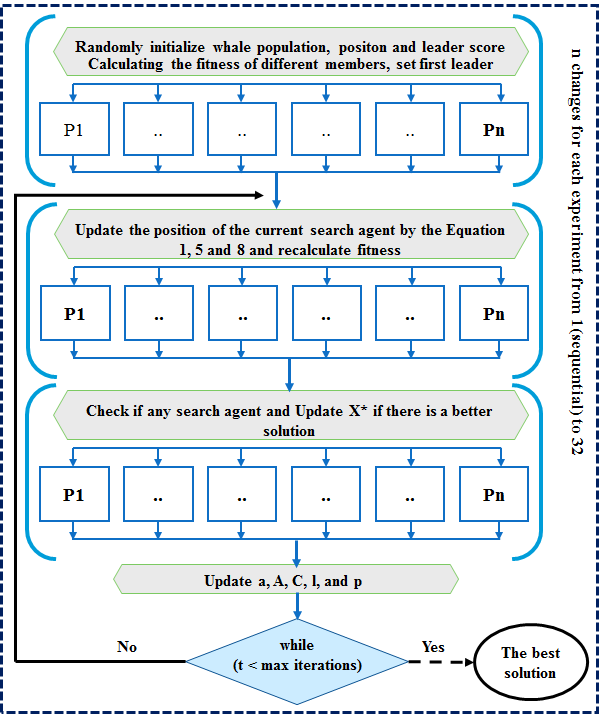
Figure 1: The flow diagram of PWOA.

4 Experimental Results and Discussion

This section will introduce the experimental results to evaluate the performance of the proposed PWOA algorithm. For each function, the PWOA algorithm was run using the parameters depicted in Table 3.

Table 3: Parameters setting of PWOA.

Parameter	Value
Number of Processors	1:32
Number of Runs	30
Number of Generations	500
Number of Populations	30

4.1 Performance Measurements

Three performance measurements, time, speed up, and efficiency are utilized to measures the performance of the proposed PWOA algorithm.

Speedup:

Speedup measures the ration between the sequential execution time and the parallel execution time and obtained as follows:

$$S(P)=\ \frac{T(1)}{T(N)}$$ (14)

Where, $T(1)$ is the execution time with one processor and $T(N)$ is the execution time with $N$ processors.

Efficiency:

Efficiency is the ration between performance and the resources used to achieve that performance. Also it measures the usage of the computational resources and calculating by the following Equation.

$$E(N)=\ \frac{S(N)}{N}$$ (15)

Where, $S(N)$ is the speedup for $N$ processors.

4.2 Results and Discussion

We evaluated the proposed novel version of the parallel WOA implementation on a ‘classical’ benchmark which comprised a set of functions and optimization problems which are often used to evaluate stochastic optimization algorithms.

Table 5 and Table 4,presents the comparison between the results for each unconstrained function on different number of processors.

Table 4: the average results for each unconstrained unimodal benchmark functions on different processors.

Uni	1 pr avg	2 pr avg	4 Pr avg	8 Pr avg	16 Pr avg	32 Pr avg
F1	0	0	0	0	0	0
F2	0	0.072074	0.054917	0.043621	0.033433	0.019102
F3	0.079938	0.103134	0.151403	0.111385	0.156628	0.156449
F4	0.000185	0.062434	0.184934	0.101786	0.169903	0.167528
F5	24.7332	25.30602	26.11116	26.02233	25.85528	25.96711
F6	0.002263	0.127186	0.196034	0.195236	0.213673	0.178586
F7	0.311751	0.171542	0.205471	0.191338	0.151258	0.209223

Table 5: the the average results for each unconstrained multimodal benchmark functions on different processors.

Uni	1 pr avg	2 pr avg	4 Pr avg	8 Pr avg	16 Pr avg	32 Pr avg
F8	-12565.6	-11116.9	-9704.73	-9688.25	-10431.9	-11110.2
F9	0	0.031745	0.021057	0.020036	0.033443	0.018585
F10	2.81E-15	0.063487	0.041188	0.031537	0.016977	0.036255
F11	-1.02131	-0.93397	-0.8071	-0.87707	-0.87715	-0.85914
F12	0.020837	0.247476	0.214033	0.219846	0.238623	0.233929
F13	0.000514	0.051837	0.032604	0.022862	0.031467	0.074587
F14	-1	-1	-1	-1	-1	-1
F15	0	0	0	0	0	0
F16	0	0	0	0	0	0
F17	2.01E-06	2.09E-06	1.11E-06	9.57E-07	3.28E-07	4.95E-06
F18	0	0	0	0	0	0
F19	0	0	0	0	0	0
F20	0	0	0	0	0	0

Table 6, presents the optimization comparison results obtained for the constrained engineering optimization problems over different number of processors.

Table 6: the average result for each constrained optimization problem on different processors (P).

Uni	1 pr avg	2 pr avg	4 Pr avg	8 Pr avg	16 Pr avg	32 Pr avg
Gear Train	6.60E-21	2.33E-19	1.65E-22	2.72E-20	2.72E-20	4.30E-20
Cantilever beam	13.03263	13.03258	13.03253	13.03255	13.03258	13.03253
Himmelblau	-30288.6	-30288.6	-30288.6	-30288.6	-30288.6	-30288.6
Constraint	707.1735	707.458	707.3283	707.2103	707.2301	707.1876
Constraint	-1.16168	-1.17116	-1.17426	-1.17431	-1.17419	-1.17426

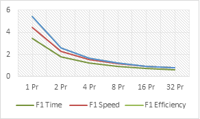
(a) Function 1.

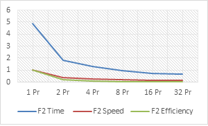
(b) Function 2.

Figure 2: The graphical results obtained by the proposed PWOA algorithm in terms of time, speedup, and efficiency for different number of processors for each unconstrained multimodal benchmark functions from Function 1 to Function 2.

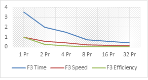
(a) Function 3.

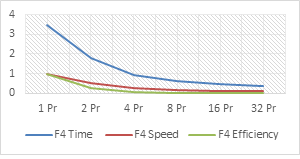
(b) Function 4.

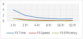
(c) Function 5.

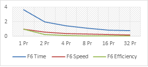
(d) Function 6.

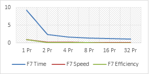
(e) Function 7.

Figure 3: The graphical results obtained by the proposed PWOA algorithm in terms of time, speedup, and efficiency for different number of processors for each unconstrained multimodal benchmark functions from Function 3 to Function 7.

Figure 2 and 3 shows the graphical results for the proposed PWOA algorithm in terms of time, speedup, and efficiency for different number of processors for each unconstrained unimodal benchmark functions. The execution time changing dependent on the problem dimension. This happens because of the limited internal resources can dedicate to each thread (processor). its clear from Figure 2 and 3, the time, speed up and efficiency starts with high value associated with Pr1 and decreases proportionally when the number of processors increases.

Therefore, we have examined alternative solutions to solve the optimization problems. A parallel WOA is designed to deal with high-dimensional problems while allowing one to run each stage of a swarm (whale) in parallel. Even when one swarm (whale) is to be engaged, the full advantage of the parallel computation could be utilized, this an observation related to PWOA. Meanwhile, the parallelism cannot be utilized in computing the objective (fitness) function in this design. Whereas the fitness computation must be implemented as a sequential process associated to the swarm within the thread, subsequently, in such case of large-scale optimization problems PWOA becomes a very promising tool, according to the large amounts of computation and data.

Figure 4 and 5shows the graphical results for the proposed PWOA algorithm in terms of time, speedup, and efficiency for different number of processors for each unconstrained multimodal benchmark functions.

Also, Figure 6 shows the graphical results for the proposed PWOA algorithm in terms of time, speedup, and efficiency for different number of processors for each constrained optimization problems.

Actually, in most of the sequential evolutionary algorithms, the fitness considered as the significant task in which the performance of the algorithm depending on it as well as WOA. So, the number of fitness evaluations is the most primary measure of the execution time. In particular, we observed that the proposed PWOA, has achieved a better performance in terms of the time, speed up and efficiency when the number of processors increases.

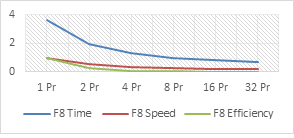
(a) Function 8.

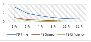
(b) Function 9.

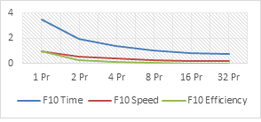
(c) Function 10.

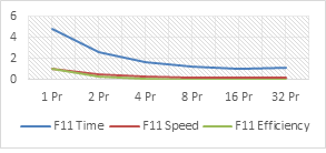
(d) Function 11.

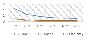
(e) Function 12.

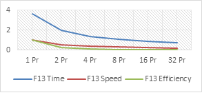
(f) Function 13.

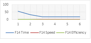
(g) Function 14.

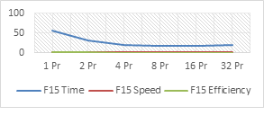
(h) Function 15.

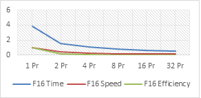
(i) Function 16.

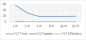
(j) Function 17.

Figure 4: The graphical results obtained by the proposed PWOA algorithm in terms of time, speedup, and efficiency for different number of processors for each unconstrained multimodal benchmark functions from F8 to F17.

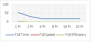
(a) Function 18.

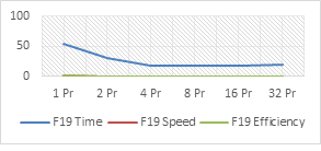
(b) Function 19.

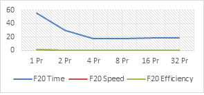
(c) Function 20.

Figure 5: The graphical results obtained by the proposed PWOA algorithm in terms of time, speedup, and efficiency for different number of processors for each unconstrained multimodal benchmark functions from F18 to F20.

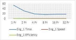
(a) Optimization problem 1.

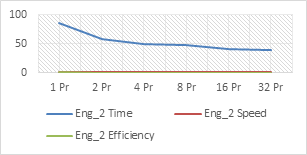
(b) Optimization problem 2.

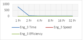
(c) Optimization problem 3.

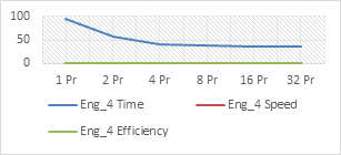
(d) Optimization problem 4.

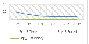
(e) Optimization problem 5.

Figure 6: The graphical results for the proposed PWOA algorithm in terms of time, speedup, and efficiency for different number of processors for each constrained optimization problems.

5 Conclusion

Recently, the huge development for the parallel computational techniques and rapid increasing in the complex optimization problems in which are composed of performing many amounts of calculations. According to the aforementioned, in this paper, a novel parallel whale optimization algorithm (PWOA) is proposed, in order to enhance the WOA performance for solving optimization problems. The completed implementation was tested using 20 constrained benchmark functions and 5 unconstrained optimization problems. However, the time required to solve large-scale optimization problem was reduced extraordinarily by utilizing the parallel computation exhibiting multiple local minima. The experimental results have verified that PWOA has achieved a good performance in terms of the time, speed up and the efficiency. Furthermore, the proposed parallel algorithm based on OpenMP greatly improved the performance compared with the basic WOA and fully demonstrates the powerful calculating capacity of parallel processing. the proposed algorithm is an efficient algorithm for image processing, classification and great significance in improving the performance of intelligence systems dealing with big data and large-scale optimization problem. The future study will focus on hybrid recent swarm optimization algorithm in terms of the similar method presented in the paper in order to eliminate wasted CPU cycles via a dynamic task queue.

References

- [1] A. E. Hassanien, E. Emary, Swarm intelligence: principles, advances, and applications, CRC Press, 2016.
- [2] L. Davis, Handbook of genetic algorithms.
- [3] W. Banzhaf, P. Nordin, R. E. Keller, F. D. Francone, Genetic programming: an introduction, Vol. 1, Morgan Kaufmann San Francisco, 1998.
- [4] H.-P. Schwefel, Numerische optimierung von computermodellen mittels der evolutionsstrategie, Vol. 1, Birkha¨user, Basel Switzerland, 1977.
- [5] D. Dasgupta, Z. Michalewicz, Evolutionary algorithms in engineering applications, Springer Science & Business Media, 2013.
- [6] D. Simon, Biogeography-based optimization, IEEE transactions on evolutionary computation 12 (6) (2008) 702–713.
- [7] R. A. Formato, Central force optimization: a new metaheuristic with applications in applied electromagnetics, Progress In Electromagnetics Research 77 (2007) 425–491.
- [8] B. Webster, P. J. Bernhard, A local search optimization algorithm based on natural principles of gravitation, Tech. rep. (2003)
- [9] E. Rashedi, H. Nezamabadi-Pour, S. Saryazdi, Gsa: a gravitational search algorithm, Information sciences 179 (13) (2009) 2232–2248.
- [10] A. Kaveh, S. Talatahari, A novel heuristic optimization method: charged system search, Acta Mechanica 213 (3) (2010) 267–289.
- [11] ] S. He, Q. H. Wu, J. Saunders, Group search optimizer: an optimization algorithm inspired by animal searching behavior, IEEE transactions on evolutionary computation 13 (5) (2009) 973–990.
- [12] ] Z. W. Geem, J. H. Kim, G. Loganathan, A new heuristic optimization algorithm: harmony search, Simulation 76 (2) (2001) 60–68.
- [13] R. Rao, V. J. Savsani, D. Vakharia, Teaching–learning-based optimization: an optimization method for continuous non-linear large scale problems, Information Sciences 183 (1) (2012) 1–15.
- [14] J. Kennedy, Particle swarm optimization, in: Encyclopedia of machine learning, Springer, 2011, pp. 760–766.
- [15] M. Dorigo, M. Birattari, T. Stutzle, Ant colony optimization, IEEE computational intelligence magazine 1 (4) (2006) 28–39.
- [16] S. Mirjalili, The ant lion optimizer, Advances in Engineering Software 83 (2015) 80–98.
- [17] S. Mirjalili, Dragonfly algorithm: a new meta-heuristic optimization technique for solving single-objective, discrete, and multi-objective problems, Neural Computing and Applications 27 (4) (2016) 1053–1073.
- [18] S. Mirjalili, Moth-flame optimization algorithm: A novel nature-inspired heuristic paradigm, Knowledge-Based Systems 89 (2015) 228–249.
- [19] S. Mirjalili, A. Lewis, The whale optimization algorithm, Advances in Engineering Software 95 (2016) 51–67.
- [20] W. A. Watkins, W. E. Schevill, Aerial observation of feeding behavior in four baleen whales: Eubalaena glacialis, balaenoptera borealis, megaptera novaeangliae, and balaenoptera physalus, Journal of Mammalogy 60 (1) (1979) 155–163.
- [21] J. A. Goldbogen, A. S. Friedlaender, J. Calambokidis, M. F. Mckenna, M. Simon, D. P. Nowacek, Integrative approaches to the study of baleen whale diving behavior, feeding performance, and foraging ecology, BioScience 63 (2) (2013) 90–100.
- [22] J. Cao, H. Cui, H. Shi, L. Jiao, Big data: A parallel particle swarm optimization-back-propagation neural network algorithm based on mapreduce, PLoS One 11 (6) (2016) e0157551.
- [23] C. K. Filelis-Papadopoulos, G. A. Gravvanis, Parallel multigrid algorithms based on generic approximate sparse inverses: an smp approach, The Journal of Supercomputing 67 (2) (2014) 384–407.
- [24] O. Pantal´e, Parallelization of an object-oriented fem dynamics code: influence of the strategies on the speedup, Advances in Engineering Software 36 (6) (2005) 361–373.
- [25] E. L. Turner, H. Hu, A parallel cfd rotor code using openmp, Advances in Engineering Software 32 (8) (2001) 665–671.
- [26] B. Chapman, G. Jost, R. Van Der Pas, Using OpenMP: portable shared memory parallel programming, Vol. 10, MIT press, 2008.
- [27] R. Chandra, Parallel programming in OpenMP, Morgan kaufmann, 2001.
- [28] P. Jarzebski, K. Wisniewski, R. Taylor, On parallelization of the loop over elements in feap, Computational Mechanics 56 (1) (2015) 77–86.
- [29] J. G. Digalakis, K. G. Margaritis, On benchmarking functions for genetic algorithms, International journal of computer mathematics 77 (4) (2001) 481–506.
- [30] X.-S. Yang, Firefly algorithm, stochastic test functions and design optimisation, International Journal of Bio-Inspired Computation 2 (2) (2010) 78–84.
- [31] A. Askarzadeh, A novel metaheuristic method for solving constrained engineering optimization problems: crow search algorithm, Computers & Structures 169 (2016) 1–12.
- [32] H. Chickermane, H. Gea, Structural optimization using a new local approximation method, International journal for numerical methods in engineering 39 (5) (1996) 829–846.
- [33] D. M. Himmelblau, Applied nonlinear programming, McGrawHill Companies, 1972.
- [34] K. S. Lee, Z. W. Geem, A new meta-heuristic algorithm for continuous engineering optimization: harmony search theory and practice, Computer methods in applied mechanics and engineering 194 (36) (2005) 3902–3933.
- [35] A. Kaveh, S. Talatahari, A particle swarm ant colony optimization for truss structures with discrete variables, Journal of Constructional Steel Research 65 (8) (2009) 1558–1568.