Deorbitalized meta-GGA Exchange-Correlation Functionals in Solids

Abstract

A procedure for removing explicit orbital dependence from meta-generalized-gradient approximation (mGGA) exchange-correlation functionals by converting them into Laplacian-dependent functionals recently was developed by us and shown to be successful in molecules. It uses an approximate kinetic energy density functional (KEDF) parametrized to Kohn-Sham results (not experimental data) on a small training set. Here we present extensive validation calculations on periodic solids that demonstrate that the same deorbitalization with the same parametrization also is successful for those extended systems. Because of the number of stringent constraints used in its construction and its recent prominence, our focus is on the SCAN meta-GGA. Coded in vasp, the deorbitalized version, SCAN-L, can be as much as a factor of three faster than original SCAN, a potentially significant gain for large-scale ab initio molecular dynamics.

I Background and Motivation

Accuracy, generality, and computational cost are competing priorities in the unrelenting search for theoretical constructs on which to base predictive condensed matter calculations. A critical problem is to predict the stable zero-temperature lattice structure of a crystal, its cohesive energy, its bulk modulus, and fundamental gap. Treatment of other physical properties (e.g., phonon spectra, transport coefficients, response functions, etc.) is, in principle at least, built upon ingredients drawn from solution of that central problem.

Beginning about four decades ago, the dominant paradigm which emerged for treating that central problem is density functional theory (DFT) HK ; Levy79 ; Lieb83 in its Kohn-Sham (KS) KS ; EngelDreizlerBuch form. For an $N_{e}$ electron system, the KS procedure recasts the DFT variational problem as one for a counterpart non-interacting system which has its minimum at the physical system ground state energy $E_{0}$ and electron number density $n_{0}({\mathbf{r}})$. The computational problem is to solve the KS equation

$$\{-\tfrac{1}{2}\nabla^{2}+v_{\mathrm{KS}}([n];{\mathbf{r}})\}\varphi_{i}({\mathbf{r}})=\epsilon_{i}\varphi_{i}({\mathbf{r}})\;.$$ (1)

(in Hartree atomic units). The KS potential is

$$v_{\rm KS}=\delta(E_{\rm Ne}+E_{\rm H}+E_{\rm xc})/\delta n\equiv v_{\mathrm{ext}}+v_{\mathrm{H}}+v_{\mathrm{xc}}$$ (2)

where we have assumed, as appropriate for clamped nucleus solids, that the external potential, $v_{\mathrm{ext}}=\delta E_{\rm Ne}/\delta n$, is from nuclear-electron attraction. The electron-electron Coulomb interaction energy customarily is partitioned as shown, namely the classical Coulomb repulsion (Hartree energy), $E_{\mathrm{H}}$, and the residual exchange-correlation (XC) piece $E_{\mathrm{xc}}$. Note that $E_{\mathrm{xc}}$ also contains the kinetic energy correlation contribution, namely the difference between the interacting and non-interacting system kinetic energies ($T$ and $T_{s}$ respectively).

The only term of this problem which is not known explicitly is $E_{\mathrm{xc}}$. Great effort has gone into constructing approximations to it. A convenient classification, the Perdew-Schmidt Jacob’s ladder PerdewSchmidt01 , proceeds by the number and type of ingredients, e.g. spatial derivatives, non-interacting kinetic energy density, exact exchange, etc. For present purposes the pertinent rungs of that ladder are the generalized gradient approximation (GGA; dependent upon $n({\mathbf{r}})$ and $\nabla n({\mathbf{r}})$) and meta-GGA functionals, which also depend upon the non-interacting KE density,

$$t^{\mathrm{orb}}_{\rm s}({\mathbf{r}}):=\tfrac{1}{2}\sum_{i=1}^{N_{e}}|\nabla\varphi_{i}({\mathbf{r}})|^{2}\;.$$ (3)

(For simplicity of exposition, we have assumed unit occupancy and no degeneracy of KS orbitals.)

Most often (but not universally) mGGA XC functionals use $t^{\mathrm{orb}}_{\rm s}$ in the combination

$$\alpha[n]:=(t_{\mathrm{s}}^{\mathrm{orb}}[n]-t_{W}[n])/t_{TF}[n]:=t_{\theta}/t_{TF}\vspace{-2pt}$$ (4)

as a way to detect chemically distinct spatial regions SunXiaoRuzsinszky12 . The other ingredients in $\alpha[n]$ are the Thomas-Fermi Thomas ; Fermi and von Weizsäcker Weizsacker KE densities:

$$t_{TF} = c_{TF}n^{5/3}({\mathbf{r}})\;\;\;,\;\;\;c_{TF}:=\frac{3}{10}(3\pi^{2})^{2/3}$$ (5)

$$t_{W} = \frac{5}{3}t_{TF}s^{2}\;.$$ (6)

The dimensionless reduced density gradient used in GGAs and mGGAs is

$$s:=\frac{|\nabla n({\mathbf{r}})|}{2(3\pi^{2})^{1/3}n^{4/3}({\mathbf{r}})}\;.$$ (7)

Because $\alpha[n]$ is explicitly orbital dependent, the mGGA XC potential, $v_{\mathrm{xc}}=\delta E_{\mathrm{xc}}/\delta n$ is not calculable directly but instead must be obtained as an optimized effective potential (OEP) StadeleMajewskiVoglGoerling1997 ; GraboKreibichGross1997 ; GraboKreibachKurthGross2000 ; HesselmannGoerling2008 . The computational cost of OEP calculations is high enough that the procedure rarely is used in practice. Instead the so-called generalized Kohn-Sham (gKS) scheme is used. In gKS, the variational procedure is done with respect to the orbitals, not $n$. That delivers a set of non-local potentials $\delta E_{\mathrm{xc}}/\delta{\varphi_{i}}$ rather than the local $v_{\mathrm{xc}}$. For a mGGA, the KS and gKS schemes are inequivalent YangPengSunPerdewGKSBandGap2016 , a matter of both conceptual and practical consequences.

Very recently we have shown DMRSBTPRA2017 that it is possible, at least for molecules, to convert several successful mGGAs to Laplacian-level XC functionals, mGGA-L, by a constraint-based deorbitalization strategy. The scheme is to evaluate $\alpha[n]$ with an orbital-independent approximation for $t_{\theta}$, i.e., for $t_{\mathrm{s}}^{\mathrm{orb}}[n]$. This is done with a KE density functional (KEDF) that is parametrized to KS calculations on a small data set (18 atoms). The parametrization is required to satisfy known constraints on the KE density. When tested against standard molecular datasets for a considerable variety of properties, the deorbitalized (Laplacian-level) versions of three well-known meta-GGAs, MVS MVS2015 , TPSS TPSSa , and SCAN SCAN , gave as good or better results than the originals. Details are in Ref. DMRSBTPRA2017, .

An obvious, crucial challenge is whether the identical deorbitalization of a mGGA can deliver equally satisfactory results on bulk solid validation tests. If that were to be true, then the deorbitalization strategy would be validated as truly successful in that it is general for ground states, not restricted to a particular state of aggregation. Here we focus on the SCAN SCAN functional because of recent intense exploration of its broad efficacy on a considerable variety of molecular and solid systems. In short, we show that indeed SCAN-L, the deorbitalized SCAN, is essentially as accurate on a variety of solid validation tests as the original SCAN. The deorbitalization strategy thus is validated as general, not specific to finite, self-bound systems.

In order, the sections which follow give computational details (Sect. II), numerical results (Sect. III), interpretive comparison of original and deorbitalized quantities such as $\alpha[n]$ (Sect. IV), computational performance (Sect. V), and brief conclusions (Sect. VI).

II Computational details

The deorbitalized SCAN (SCAN-L) used in all calculations is precisely the form and parametrization given in Ref. DMRSBTPRA2017, .

All computations presented in this work were performed with a locally modified version of the Vienna ab initio Simulation Package (vasp). Two separate implementations of the deorbitalized scheme were coded. One used the mGGA trunk of vasp, modified as necessary to handle the Laplacian-dependence. That included use of the KS rather than gKS solution. The second version used the GGA trunk, augmented to include the Laplacian in the one place it appears, $\alpha[n]$, and its derivative appearance in $v_{\mathrm{KS}}$. These coding differences have pronounced computational performance consequences, as discussed in Sect. V.

The PAW data sets utilized correspond to the PBE 5.4 package and are summarized in Table 1. We note that the use of inconsistent PAW data sets (PBE with SCAN) follows precedent. To our knowledge there is no alternative; no SCAN-based PAW data set is available for vasp. These PAW data sets contain information about the core kinetic energy density needed by SCAN SCAN . There are two exceptions, H and Li, for which the selected PAW data sets are all-electron but violate the requirement given in the VASP Wiki VASPwiki . We found, nevertheless, that the equilibrium lattice constants for LiH, LiF, and LiCl from an equation of state fitted (see below) to calculations that used those PAW data sets are quite sensible. It is important to mention that in order to obtain the same equilibrium lattice constants from the stress tensor values as from the equation of state fitting the patch #1 VASPpatch needs to be applied to VASP.

The default energy cutoff (vasp variable ENCUT) was overridden and set to 800 eV, except for calculations involving Li. In those, the cutoff was increased to 1000 eV for LiCl and LiF, and to 1200 eV for Li.

The precision parameter in vasp was set to “accurate” (PREC=A) and the minimization algorithm used an “all-band simultaneous update of orbitals” conjugate gradient method (ALGO=A). Non-spherical contributions within the PAW spheres were included self-consistently (LASPH=.TRUE.).

For hexagonal close-packed structures we used the ideal $c/a$ ratio. For graphite and hexagonal boron nitride, we fixed the intralayer lattice constant to its experimental value and varied the interlayer lattice constant only.

Brillouin zone integrations were performed on ($17\times 17\times 17$) $\Gamma$-centered symmetry reduced Monkhorst-Pack MonkhorstPack $k$-meshes using the tetrahedron method with Blöchl corrections Bloechl .

The equilibrium lattice constants $a_{0}$ and bulk moduli $B_{0}$ at $T=0K$ were determined by calculating the total energy per unit cell in the range $V_{0}\pm 10\%$ (where $V_{0}$ is the equilibrium unit cell volume), followed by a twelve-point-fit to the stabilized jellium equation of state (SJEOS) SJEOS . The SJEOS is

$$E(V)=\alpha\left(\frac{V_{0}}{V}\right)+\beta\left(\frac{V_{0}}{V}\right)^{2/3}+\gamma\left(\frac{V_{0}}{V}\right)^{1/3}+\omega\;.$$ (8)

A linear fit to Eq, (8) yields parameters $\alpha_{s}=\alpha V_{0}$, $\beta_{s}=\beta V_{0}^{2/3}$, $\gamma_{s}=\gamma V_{0}^{1/3}$ and $\omega$, from which

$$V_{0}=\left(\frac{-\beta_{s}+\sqrt{\beta_{s}^{2}-3\alpha_{s}\gamma_{s}}}{\gamma_{s}}\right)^{3}\;,$$ (9)

$$B_{0}=\frac{18\alpha+10\beta+4\gamma}{9V_{0}}\;.$$ (10)

To obtain cohesive energies, approximate isolated atom energies were calculated from a $14\times 15\times 16$ ų cell. The lowest energy configuration was sought by allowing spin-polarization and breaking spherical symmetry, but without spin-orbit coupling.

III Numerical Results

Table 3 compares static-crystal lattice constants and cohesive energies of 55 solids and Table 4 compares bulk moduli of 44 solids computed with the orbital-dependent SCAN and its deorbitalized version SCAN-L. Experimental values shown in Table 3 were taken from Ref. SCAN+rVV10, . Those in Table 4 were taken from Ref. TranStelzlBlaha, . The overall excellent agreement between the values obtained with SCAN and SCAN-L for all three properties indicate that SCAN-L provides a faithful reproduction of the SCAN potential energy surfaces near equilibrium for these systems. Figure 1 depicts the correlation between SCAN and SCAN-L results for each of the three properties.

Outliers differing more than $\pm 10\%$ are indicated by their chemical symbol. It is readily apparent from Figure 1 that SCAN-L predicts Pt, Rh and Ir to be more compressible than does the original SCAN functional. On the other hand, SCAN-L predicts Al, LiCl, K, and Rb to be less compressible (these solids are not highlighted in Figure 1 due to cluttering). At the resolution of that figure, there are no serious outliers for equilibrium lattice constant. In fact, the differences between lattice constants predicted by SCAN and SCAN-L are $1\%$ or less for each one of the solids. There are a few outliers in the cohesive energies set. However, it is notable that there is no systematic under- or overbinding from SCAN-L with respect to SCAN values of $E_{coh}$. The ground-state configurations of all elements were the same with SCAN and SCAN-L, however, we must note that one must start from a previously converged PBE density to obtain the lowest lying state of Hf with SCAN-L.

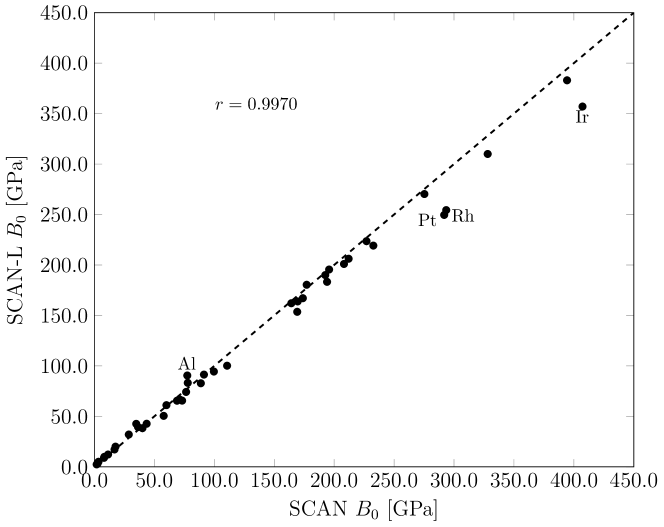
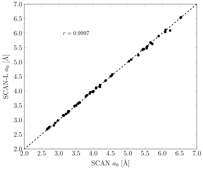
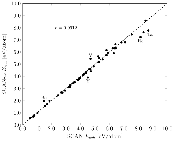
Figure 1: Comparison between SCAN and SCAN-L bulk moduli $B_{0}$ (top), static-crystal lattice constants $a_{0}$ (middle), and cohesive energies $E_{coh}$ (bottom). A dashed line with slope $1$ and Pearson correlation coefficient $r$ is shown in each of the three plots.

Table 5 displays KS band gaps for SCAN-L compared to those from SCAN. As expected, the SCAN-L band gap values always are less than or equal to those from the orbital-dependent SCAN. This systematic difference arises because the exchange-correlation potential of SCAN-L is a local multiplicative one, whereas the one from orbital-dependent SCAN is non-multiplicative SCAN+BG . In other words, the difference in KS band gaps is a direct consequence of the difference between KS and generalized gKS methods. If SCAN-L is a faithful deorbitalization of SCAN, then the SCAN-L exchange-correlation potential should be a good approximation to the SCAN OEP (which, so far as we know, has not been generated for any solid), Thus, the SCAN-L KS band gaps should agree reasonably well with the values obtained in Ref. SCAN+BG, for the Krieger-Li-Iafrate (KLI) approximation to the OEP of SCAN. To facilitate such comparison, Table 5 shows both the “SCAN(BAND)” and “SCAN(KLI)” band gaps reported in Ref. SCAN+BG, . “SCAN(BAND)” results are all-electron gKS values from the BAND code BANDcode . The SCAN band gaps computed here with vasp and PAWs are smaller than those obtained with the BAND code as reported in Ref. SCAN+BG, . Presumably that is a consequence of the PAWs and the difference in basis sets. However, there is no systematic deviation of the SCAN-L KS band gaps from the SCAN(KLI) ones. Most are close, with the two outliers, in a relative sense, being GaAs and InP: 0.33 eV and 0.59 eV from SCAN-L versus 0.45 eV and 0.77 eV from SCAN(KLI), respectively. It therefore seems that the SCAN-L potential is at least a reasonably good approximation to the SCAN OEP.

One of the features of SCAN that has been emphasized in the literature is its ability to capture intermediate-distance correlation effects in weakly bonded systems such as graphite and hexagonal boron nitride (h-BN) SCAN+rVV10 ; SCANNature . Table 6 shows the interlayer binding energy $E_{b}$ and interlayer lattice constant $c$ for these two systems from SCAN and SCAN-L as well as reference values from Ref. SCAN+rVV10, . $E_{b}$ is small, thus particularly sensitive to formal and computational differences. Nevertheless SCAN-L reproduces the SCAN $E_{b}$ result for graphite and h-BN to less than 5.0% discrepancy. The SCAN-L $c$ values are somewhat closer to the reference ones but still agree to less than 2.5% difference with the SCAN ones. Note, however, that our SCAN binding energies for Graphite and h-BN are 10% smaller than those reported in Reference [SCAN+rVV10, ].

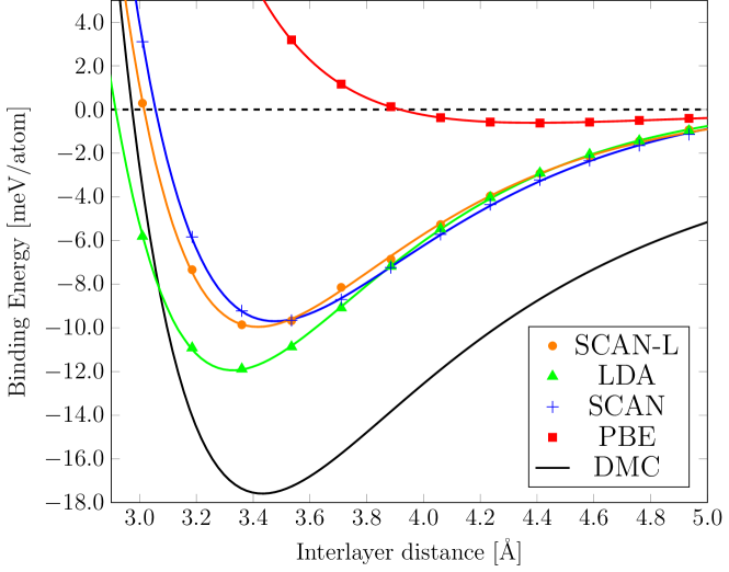
Figure 2: Graphene bilayer interplanar binding (meV/atom) as computed with LDA, PBE, SCAN, and SCAN-L XC functionals. A fit to diffusion quantum Monte Carlo (DMC) data DMC is shown as reference.

It is also significant for use of van der Waals correctionsSCAN+rVV10 ; HermannTkatchenko that SCAN-L reproduces the SCAN binding curve $E_{b}(c)$ for a bilayer of graphene (BLG) quite well. In Fig. 2 we show the binding curves for LDA, PBE PBE , SCAN and SCAN-L XC functionals compared to a diffusion quantum Monte Carlo (DMC) reference DMC . The SCAN-L functional is able to recover the binding “lost” by PBE and other GGA-type functionals. The interlayer separation predicted by SCAN (3.48 Å) and SCAN-L (3.41 Å) are in good agreement to the DMC-fit prediction (3.42 Å).

Table 1: PAWs used in the present work. The energy cutoffs $E_{cut}$ (eV) shown are the default for each PAW and were overridden as discussed in the text.

Element	Name	Valence	$E_{cut}$
H	H_h_GW	$1s$	700
Li	Li_AE_GW	$1s2s$	433
B	B	$2s2p$	319
C	C_GW_new	$2s2p$	414
N	N_GW_new	$2s2p$	421
O	O_GW_new	$2s2p$	434
F	F_GW_new	$2s2p$	487
Na	Na_pv	$2p3s$	373
Mg	Mg_sv_GW	$2s2p3s$	430
Al	Al_GW	$3s3p$	240
Si	Si_GW	$3s3p$	547
P	P_GW	$3s3p$	255
S	S_GW	$3s3p$	259
Cl	Cl_GW	$3s3p$	262
K	K_pv	$3p4s$	249
Ca	Ca_pv	$3p4s$	119
Sc	Sc_sv_GW	$3s3p3d4s$	379
Ti	Ti_sv_GW	$3s3p3d4s$	384
V	V_sv_GW	$3s3p3d4s$	382
Fe	Fe_sv_GW	$3s3p3d4s$	388
Co	Co_sv_GW	$3s3p3d4s$	387
Ni	Ni_sv_GW	$3s3p3d4s$	390
Cu	Cu_GW	$3d4s$	417
Ga	Ga_d_GW	$3d4s4p$	404
Ge	Ge_d_GW	$3d4s4p$	375
As	As_GW	$4s4p$	208
Rb	Rb_sv	$4s4p5s$	424
Sr	Sr_sv	$4s4p5s$	229
Y	Y_sv_GW	$4s4p4d5s$	340
Zr	Zr_sv_GW	$4s4p4d5s$	346
Nb	Nb_sv_GW	$4s4p4d5s$	354
Mo	Mo_sv_GW	$4s4p4d5s$	345
Tc	Tc_sv_GW	$4s4p4d5s$	351
Ru	Ru_sv_GW	$4s4p4d5s$	348
Rh	Rh_sv_GW	$4s4p4d5s$	351
Pd	Pd_pv	$4p4d5s$	250
Ag	Ag_GW	$4d5s$	250
In	In_d_GW	$4d5s5p$	279
Sn	Sn_d_GW	$4d5s5p$	260
Sb	Sb_GW	$5s5p$	172
Cs	Cs_sv_GW	$5s5p6s$	198
Ba	Ba_sv_GW	$5s5p6s$	237
Hf	Hf_sv_GW	$5p6s6d$	283
Ta	Ta_sv_GW	$5p6s6d$	286
W	W_sv_GW	$5p5d6s$	317
Re	Re_sv_GW	$5p5d6s$	317
Os	Os_sv_GW	$5p5d6s$	320
Ir	Ir_sv_GW	$5p5d6s$	320
Pt	Pt_pv	$5p5d6s$	295
Au	Au_GW	$5d6s$	248

Table 2: Strukturbericht symbols of the 57 solids used in the present work: A1 face-centered cubic, A2 body-centered cubic, A3 hexagonal close-packed, A9 hexagonal unbuckled graphite, B1 rock salt, B3 zinc blende, and B_k hexagonal boron nitride.

Solid	Symbol	Solid	Symbol	Solid	Symbol
C	A4	NaF	B1	Hf	A3
Si	A4	NaCl	B1	V	A2
Ge	A4	MgO	B1	Nb	A2
Sn	A4	Li	A2	Ta	A2
SiC	B3	Na	A2	Mo	A2
BN	B3	K	A2	W	A2
BP	B3	Rb	A2	Tc	A3
AlN	B3	Cs	A2	Re	A3
AlP	B3	Ca	A1	Ru	A3
AlAs	B3	Ba	A2	Os	A3
GaN	B3	Sr	A1	Rh	A1
GaP	B3	Al	A1	Ir	A1
GaAs	B3	Fe	A2	Pd	A1
InP	B3	Co	A1	Pt	A1
InAs	B3	Ni	A1	Cu	A1
InSb	B3	Sc	A3	Ag	A1
LiH	B1	Y	A3	Au	A1
LiF	B1	Ti	A3	C	A9
LiCl	B1	Zr	A3	BN	Bk

Table 3: Static-lattice lattice constants, $a_{0}$ (Å), and cohesive energies, $E_{coh}$ (eV/atom), of 55 solids. The experimental values, from Ref. SCAN+rVV10, , include zero-point effects.

Solid	Experimental			SCAN			SCAN-L
	$a_{0}$	$E_{coh}$		$a_{0}$	$E_{coh}$		$a_{0}$	$E_{coh}$
C	3.553	7.55		3.551	7.55		3.567	7.44
Si	5.421	4.68		5.429	4.69		5.423	4.60
Ge	5.644	3.89		5.668	3.94		5.667	3.82
Sn	6.477	3.16		6.540	3.27		6.546	3.25
SiC	4.346	6.48		4.351	6.45		4.357	6.31
BN	3.592	6.76		3.606	6.84		3.612	6.80
BP	4.525	5.14		4.525	5.31		4.530	5.19
AlN	4.368	5.85		4.360	5.80		4.364	5.75
AlP	5.451	4.32		5.466	4.24		5.449	4.16
AlAs	5.649	3.82		5.671	3.84		5.659	3.71
GaN	4.520	4.55		4.505	4.41		4.513	4.38
GaP	5.439	3.61		5.446	3.62		5.445	3.51
GaAs	5.640	3.34		5.659	3.29		5.677	3.15
InP	5.858	3.47		5.892	3.19		5.896	3.10
InAs	6.047	3.08		6.094	2.94		6.109	2.82
InSb	6.468	2.81		6.529	2.68		6.528	2.67
LiH	3.979	2.49		3.997	2.43		3.969	2.42
LiF	3.972	4.46		3.978	4.38		3.979	4.27
LiCl	5.070	3.59		5.099	3.51		5.086	3.43
NaF	4.582	3.97		4.553	3.90		4.574	3.78
NaCl	5.569	3.34		5.563	3.26		5.542	3.18
MgO	4.189	5.20		4.194	5.24		4.205	5.17
Li	3.443	1.67		3.457	1.56		3.470	1.56
Na	4.214	1.12		4.193	1.04		4.143	0.99
K	5.212	0.94		5.305	0.81		5.238	0.78
Rb	5.577	0.86		5.710	0.74		5.626	0.69
Cs	6.039	0.81		6.227	0.53		6.090	0.57
Ca	5.556	1.87		5.546	1.87		5.476	1.98
Ba	5.002	1.91		5.034	1.48		5.027	1.96
Sr	6.040	1.73		6.084	1.71		6.040	1.71
Al	4.018	3.43		4.006	3.57		3.997	3.52
Fe	2.853	4.30		2.855	4.60		2.811	4.58
Co	3.524	4.42		3.505	4.72		3.503	4.41
Ni	3.508	4.48		3.460	5.30		3.488	5.51
Sc	3.270	3.93		3.271	3.96		3.261	3.87
Y	3.594	4.39		3.608	4.52		3.599	3.90
Ti	2.915	4.88		2.897	4.92		2.898	4.83
Zr	3.198	6.27		3.212	5.90		3.211	5.94
Hf	3.151	6.46		3.123	6.30		3.159	5.90
V	3.021	5.35		2.973	4.70		2.981	5.44
Nb	3.294	7.60		3.296	6.37		3.306	6.31
Ta	3.299	8.13		3.272	8.69		3.300	7.77
Mo	3.141	6.86		3.145	5.80		3.151	6.16
W	3.160	8.94		3.149	8.36		3.165	7.63
Tc	2.716	6.88		2.711	6.42		2.724	6.65
Re	2.744	8.05		2.730	8.15		2.761	7.23
Ru	2.669	6.77		2.663	6.23		2.681	6.31
Os	2.699	8.20		2.686	8.50		2.710	8.59
Rh	3.794	5.78		3.786	5.22		3.817	5.65
Ir	3.831	6.99		3.814	7.08		3.856	6.80
Pd	3.876	3.93		3.896	4.16		3.913	4.07
Pt	3.913	5.87		3.913	5.53		3.956	5.39
Cu	3.595	3.51		3.566	3.86		3.570	3.73
Ag	4.062	2.96		4.081	2.76		4.098	2.65
Au	4.062	3.83		4.086	3.32		4.120	3.28
ME				0.011	-0.10		0.009	-0.17
MAE				0.025	0.24		0.024	0.26
MARE (%)				0.54	5.93		0.55	6.42

Table 4: Bulk modulus, $B_{0}$ (GPa) of the 44 cubic solids. The experimental values, from Ref. TranStelzlBlaha, , were obtained by subtracting the zero-point phonon effect from the experimental zero-temperature values.

Solid	Expt.	SCAN	SCAN-L
C	454.7	459.9	442.6
Si	101.3	99.7	94.4
Ge	79.4	71.2	66.7
Sn	42.8	40.1	38.3
SiC	229.1	227.0	223.6
BN	410.2	394.3	383.0
BP	168.0	173.9	167.1
AlN	206.0	212.1	206.2
AlP	87.4	91.4	91.4
AlAs	75.0	76.5	74.2
GaN	213.7	194.1	183.3
GaP	89.6	88.8	82.8
GaAs	76.7	73.2	65.6
InP	72.0	68.9	65.5
InAs	58.6	57.8	50.5
InSb	46.1	43.6	42.7
LiH	40.1	36.4	39.4
LiF	76.3	77.9	83.2
LiCl	38.7	34.9	42.6
NaF	53.1	60.1	61.1
NaCl	27.6	28.7	32.0
MgO	169.8	169.6	163.9
Li	13.1	16.8	17.2
Na	7.9	8.0	8.9
K	3.8	3.4	5.0
Rb	3.6	2.7	3.3
Cs	2.3	1.9	2.4
Ca	15.9	17.6	20.0
Ba	10.6	8.3	9.9
Sr	12.0	11.4	12.2
Al	77.1	77.5	90.5
Ni	192.5	232.7	219.2
V	165.8	195.8	195.5
Nb	173.2	177.1	180.4
Ta	202.7	208.2	201.0
Mo	276.2	275.3	270.3
W	327.5	328.1	310.0
Rh	277.1	293.5	254.4
Ir	362.2	407.2	357.0
Pd	187.2	192.6	190.0
Pt	285.5	291.8	249.6
Cu	144.3	164.3	162.1
Ag	105.7	110.7	100.2
Au	182.0	169.2	153.6
ME		3.0	-3.0
MAE		6.9	9.2
MARE (%)		7.1	9.4

Table 5: Band gap (eV) of 21 insulators and semiconductors. Experimental lattice parameters were used with all functionals. Experimental band gaps and lattice constants were taken from Ref. TranBlahaBG, .

Solid	Expt.	SCAN	SCAN-L	SCAN(BAND)	SCAN(KLI)
C	5.50	4.54	4.22	4.58	4.26
Si	1.17	0.82	0.80	0.97	0.78
Ge	0.74	0.14	0.00
SiC	2.42	1.72	1.55
BN	6.36	4.98	4.66	5.04	4.73
BP	2.10	1.54	1.41	1.74	1.52
AlN	4.90	3.97	3.50
AlP	2.50	1.92	1.81
AlAs	2.23	1.74	1.59
GaN	3.28	1.96	1.49
GaP	2.35	1.83	1.72	1.94	1.72
GaAs	1.52	0.77	0.33	0.80	0.45
InP	1.42	1.02	0.59	1.06	0.77
InAs	0.42	0.00	0.00
InSb	0.24	0.00	0.00
LiH	4.94	3.66	3.69
LiF	14.20	10.10	9.16	9.97	9.11
LiCl	9.40	7.33	6.80
NaF	11.50	7.14	6.45
NaCl	8.50	5.99	5.59	5.86	5.25
MgO	7.83	5.79	4.92	5.62	4.80
ME		-1.26	-1.58
MAE		1.26	1.58

Table 6: Inter-layer binding energy $E_{b}$ in meV/Ų and inter-layer lattice constant $c$ in Å. The reference $E_{b}$ values are from RPA calculations and from experiments for $c$.

Solid	Reference		SCAN		SCAN-L
	$E_{b}$	$c$	$E_{b}$	$c$	$E_{b}$	$c$
Graphite	18.32	6.70	7.23	6.97	7.37	6.81
$h$-BN	14.49	6.54	7.66	6.85	7.70	6.72

Table 7: Comparative timings for PBE, SCAN, and SCAN-L calculations in the original and modified mGGA and GGA trunks of vasp. All times in seconds. See text for trunk labels.

XC	Trunk	Original	Modified
		Code	Code
PBE	GGA=PE	12.38	12.85
PBE	METAGGA=PBE	36.75	37.57
SCAN	METAGGA=SCAN	61.28	–
SCAN-L	GGA=SL	–	19.32
SCAN-L	METAGGA=SCANL	–	50.72

IV Interpretive Results

How the faithful deorbitalization is achieved in SCAN-L can be understood by how well $\alpha$ is approximated by the kinetic energy density functional utilized. Figure 3 shows the comparison between the orbital-dependent $\alpha$ Eq. (4) and the approximation that results from use of the modified PC07 kinetic energy density functional in deorbitalizing SCAN DMRSBTPRA2017 . Details of the parametrization of PC07 are in that reference. The three systems selected as examples in that Figure were chosen because they span the bonding situations among which $\alpha$ is supposed to discriminate. The BeH radical has $\alpha\approx 0$ as is true of most covalently bounded systems. The sodium dimer has $\alpha\approx 1$ as in most metallic systems. The stacked benzene dimer is representative of weakly bound systems for which $\alpha\gg 1$ is typical. The deorbitalized $\alpha$ follows its orbital-dependent counterpart closely both within and outside the bonding regions. Important differences can be noted for the benzene dimer at the mid-point of the interplanar axis. However, even though the deorbitalized $\alpha$ is almost 50 % of the exact one, the difference between SCAN and SCAN-L enhancement factors is less than 5 %. Larger differences between the exact and approximate $\alpha$s might be observed in the tails of the density. Those are almost nonexistent in condensed systems near equilibrium and they prove to be inconsequential for molecules (which is why such points are screened out in most molecular computational packages). In short, where it counts in both solids and molecules, the PC07 function reproduces the behavior of the original SCAN $\alpha$.

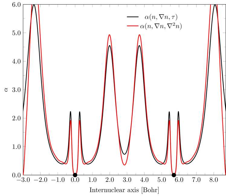
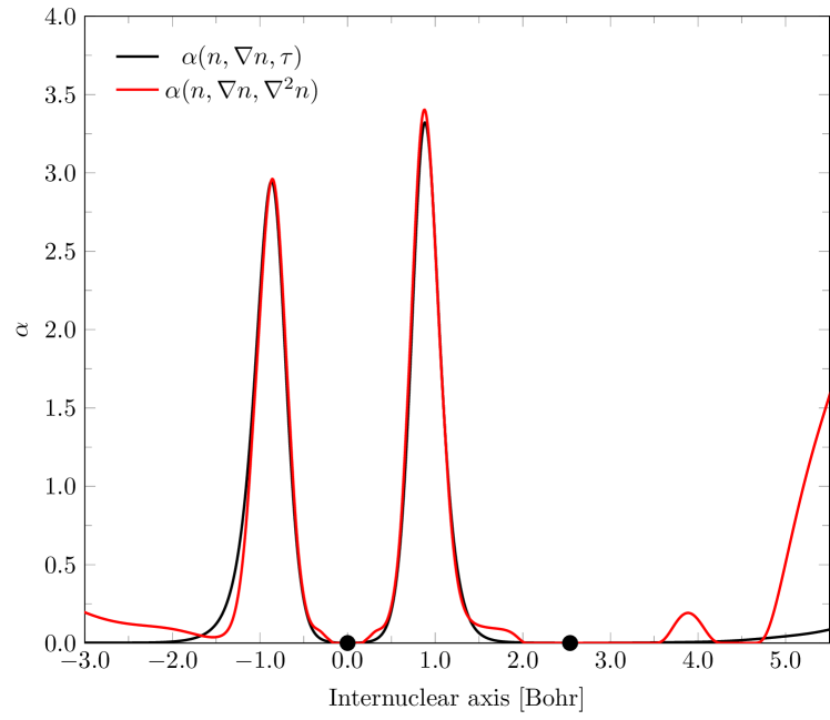
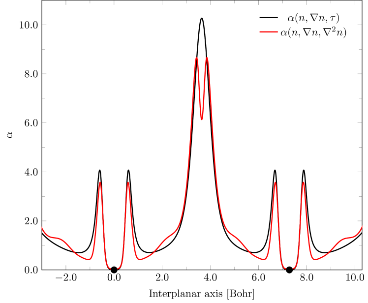
Figure 3: Orbital-dependent $\alpha$ and its deorbitalized approximation for three representative bonding situations. Na₂ (top) exemplifies systems with $\alpha\approx 1$; BeH (middle) exemplifies systems with $\alpha\approx 0$, and the benzene dimer exemplifies those with $\alpha\gg 1$.

V Computational Performance

To obtain a quantitative picture of the performance of GGA and mGGA calculations in vasp, we prepared a fully sequential (serial) version compiled in profiling mode and linked to the Intel Math Kernel and Fast Fourier Transform libraries. Two variants were compiled, original and with SCAN-L included. Within the original variant, three calculations were done: PBE using the GGA trunk (GGA=PBE), PBE using the mGGA trunk (METAGGA=PBE) and SCAN (METAGGA=SCAN). Correspondingly in the SCAN-L coded variant, the four were PBE using the extended GGA trunk (GGA=PE), PBE using the modified mGGA trunk (METAGGA=PBE), SCAN-L using the extended GGA trunk (GGA=SL) and SCAN-L using the modified mGGA trunk (METAGGA=SCANL).

The test system was diamond carbon at a lattice constant, $a_{0}$ = 3.560 Å, near the SCAN-L equilibrium value. Calculations used a 600 eV planewave cutoff, the all-bands conjugate gradient minimization (ALGO=A), aspherical corrections (LASPH=.TRUE.), doubling of the Fourier grid (ADDGRID=.TRUE.) and the tetrahedron method with Blöchl corrections (ISMEAR=-5). These are the same settings as were used for the validation studies, except for the energy cutoff. All calculations converged in 12 scf iterations.

Table 7 gives the results. Clearly the SCAN-L computational speed in the extended GGA trunk implementation is substantially superior to that for original SCAN. When using the mGGA trunk, SCAN-L performance degrades but the computation is still 20% faster than the original SCAN one.

Analysis of the detailed profiling shows that when a metaGGA functional is requested, vasp first computes results for PBE XC, but then overwrites those results with the corresponding ones from the requested mGGA XC functional. It is not clear why that is done. For mGGAs, additional time is used in computing $\nabla^{2}n$, especially on the radial grid within the PAW spheres, even if that Laplacian data actually is un-needed in the requested mGGA XC functional. (Of course, it is used in SCAN-L.) That is done in anticipation of computing the modified Becke-Johnson potential (also called Tran-Blaha 09)BJ ; TB09 if requested. Furthermore, the mGGA trunk always assumes spin-polarized densities, resulting in additional time used for spin-unpolarized systems. These three sources of wasted time make the difference between the GGA=PE and METAGGA=PBE timings.

In the original vasp version, the time difference between METAGGA=PBE and METAGGA=SCAN arises from the non-locality of the Hamiltonian of a conventional mGGA (as in SCAN). Implementing SCAN-L as an extension of the GGA trunk saves time because the associated $v_{\mathrm{KS}}$ is local. That implementation also avoids wasting time calculating un-needed PBE results and avoids treating spin unpolarized systems as spin polarized ones.

VI Conclusion

We have shown that the SCAN-L functional, a simple orbital-independent form of the sophisticated and much-advertised SCAN functional, can capture all the pertinent details of orbital-dependent functionals both in molecules and solids. We believe SCAN-L to be the first example of an orbital-independent functional that provides uniformly rather good performance in these two seemingly irreconcilable domains of aggregation. As such, SCAN-L opens the way for meta-GGA XC accuracy and reliability in orbital-free DFT simulations, a possibility that has not existed heretofore. It also opens the way for much faster ab initio molecular dynamics simulations than are possible with SCAN.

Differences between SCAN-L and SCAN KS band gaps arise as a well-understood consequence of the difference between KS and gKS solutions. The KS band gaps also provide some evidence that SCAN-L provides a reasonable approximation to the OEP for SCAN. Direct comparison with the exact OEP (rather than the KLI approximation) would be welcome. The performance of SCAN-L in combination with van der Waals correction schemes also remains to be investigated.

- (1) P. Hohenberg and W. Kohn, Phys. Rev. 136, B864 (1964).
- (2) M. Levy, Proc. Natl. Acad. Sci. USA 76, 6062 (1979).
- (3) E.H. Lieb, Int. J. Quantum Chem. 24, 243 (1983).
- (4) W. Kohn and L.J. Sham, Phys. Rev. 140, A1133 (1965).
- (5) Density Functional Theory: An Advanced Course, E. Engel and R.M. Dreizler (Springer-Verlag Berlin, Berlin, 2011) and refs. therein.
- (6) J.P. Perdew and K. Schmidt, A.I.P. Conf. Proc. 577, 1 (2001).
- (7) J. Sun, B. Xiao, and A. Ruzsinszky, J. Chem. Phys. 137, 051101 (2012).
- (8) L.H. Thomas, Proc. Cambridge Phil. Soc. 23, 542 (1927).
- (9) E. Fermi, Atti Accad. Nazl. Lincei 6, 602 (1927).
- (10) C.F. von Weizsäcker, Z. Phys. 96, 431 (1935).
- (11) M. Städele, J.A. Majewski, P. Vogl and A. Görling, Phys. Rev. Lett. 79, 2089 (1997)
- (12) T. Grabo, T. Kreibich and E.K.U. Gross, Molec. Eng. 7, 27 (1997).
- (13) T. Grabo, T. Kreibach, S. Kurth, and E.K.U. Gross, in Strong Coulomb Correlations in Electronic Structure: Beyond the Local Density Approximation, V.I. Anisimov ed. (Gordon and Breach, Tokyo, 2000) 203.
- (14) A. Heßelmann and A. Görling, Chem. Phys. Lett. 455, 110 (2008) and refs. therein.
- (15) Z-h. Yang, H. Peng, J. Sun, and J.P. Perdew, Phys. Rev. B 93, 205205 (2016)
- (16) Daniel Mejía-Rodríguez and S.B. Trickey, Phys. Rev. A 96, 052512 (2017).
- (17) J. Sun, J.P. Perdew, and A. Ruzsinszky, Proc. Nat. Acad. Sci. (USA) 112, 685 (2015).
- (18) J. Tao, J.P. Perdew, V.N. Staroverov, and G.E. Scuseria, Phys. Rev. Lett. 91, 146401 (2003).
- (19) J. Sun, A. Ruzsinszky and J.P. Perdew, Phys. Rev. Lett. 115, 036402 (2015).
- (20) http://cms.mpi.univie.ac.at/wiki/index.php/METAGGA
- (21) https://www.vasp.at/index.php/news/bugfixes/119-bugfix-patch-1-for-vasp-5-4-4-18apr17
- (22) H.J. Monkhorst and J. Pack, Phys. Rev. B 13, 5188 (1976).
- (23) P.E. Blöchl, O. Jepsen and O.K. Andersen, Phys. Rev. B 49, 16223 (1994).
- (24) A.B. Alchagirov, J.P. Perdew, J.C. Boettger, R.C. Albers and C. Fiolhais, Phys. Rev. B. 63 224115 (2001).
- (25) H. Peng, Z.-H. Yang, J.P. Perdew and J. Sun, Phys. Rev. X 6, 041005 (2016).
- (26) F. Tran, J. Stelzl and P. Blaha, J. Chem. Phys. 144, 204120 (2016).
- (27) Z.-H. Yang, H. Peng, J. Sun and J.P. Perdew, Phys. Rev. B 93, 205205 (2016).
- (28) G. te Velde and E.J. Baerends, Phys. Rev. B 44, 7888 (1991); G. Wiesenekker and E.J. Baerends, J. Phys.: Condens. Matter 3, 6721 (1991); P. H.T. Philipsen, G. te Velde, E.J. Baerends, J.A. Berger, P.L. de Boeij, M. Franchini, J.A. Groeneveld, E.S. Kadantsev, R. Klooster, F. Kootstra, P. Romaniello, D.G. Skachkov, J.G. Snijders, C.J.O. Verzijl, J.A. Celis Gil, J.M. Thijssen, G. Wiesenekker, and T. Ziegler, BAND2017, SCM, Theoretical Chemistry, Vrije Universiteit, Amsterdam, The Netherlands, 2017.
- (29) J. Sun, R.C. Remsing, Y. Zhang, Z. Sun, A. Ruzsinszky, H. Peng, Z. Yang, A. Paul, U. Waghmare, X. Wu, M.L. Klein, and J.P. Perdew, Nature Chemistry 8, 831 (2016).
- (30) F. Tran and P. Blaha, J. Phys. Chem. A 121, 3318 (2017).
- (31) J. Hermann and A. Tkatchenko, J. Chem. Theory Comput. 14, 1361 (2018).
- (32) J.P. Perdew, K. Burke and M. Ernzerhof, Phys. Rev. Lett. 77, 3865 (1996).
- (33) E. Mostaani, N.D. Drummond and V.I. Fal’ko, Phys. Rev. Lett. 115, 115501 (2015).
- (34) A.D. Becke and E.R. Johnson, J. Chem. Phys. 124, 221101 (2006).
- (35) F. Tran and P. Blaha, Phys. Rev. Lett. 102, 226401 (2009).