Excitation and control of large amplitude standing magnetization waves

Abstract

A robust approach to excitation and control of large amplitude standing magnetization waves in an easy axis ferromagnetic by starting from a ground state and passage through resonances with chirped frequency microwave or spin torque drives is proposed. The formation of these waves involves two stages, where in the first stage, a spatially uniform, precessing magnetization is created via passage through a resonance followed by a self-phase-locking (autoresonance) with a constant amplitude drive. In the second stage, the passage trough an additional resonance with a spatial modulation of the driving amplitude yields transformation of the uniform solution into a doubly phase-locked standing wave, whose amplitude is controlled by the variation of the driving frequency. The stability of this excitation process is analyzed both numerically and via Whitham’s averaged variational principle.

I I. Introduction

Because of the complexity and despite decades of studies, magnetization dynamics in ferromagnetic materials remains of interest to basic and applied research. For example, nonlinear spin waves and solitons in ferromagnetic films were studied experimentally extensively (e.g. Scott1 ; Scott2 ; Patton1 ; Patton2 ). Magnetostatic and boundary effects in such macroscopic films yield complex dispersion of the spin waves. Depending on the sign of the dispersion both bright and dark magnetic solitons were observed. The long wavelength approximation in this problem yields the nonlinear Schrodinger (NLS) model, providing a convenient theoretical basis for investigation. The NLS equation has well known traveling wave and soliton solutions, Scott , allowing interpretation of the experimentally observed magnetization dynamics.

In recent years, applications in ferromagnetic nanowires opened new perspectives in studying magnetization waveforms Braun . At the nanoscales a quasi-one-dimensional symmetry can be realized and magnetostatic effects can be reduced to additional contributions to the anisotropy Braun ; Garbou ; Kohn , which can be conveniently modeled by the Landau-Lifshitz-Gibert (LLG) equation. It is known that the one-dimensional (1D), dissipationless LLG equation, similar to the NLS equation is integrable and has a multitude of exact solutions including solitons and spatially periodic waveforms Braun ; Kosevich ; M , expected to be observed in nanowires. The simplest solitons are domain walls, which are studied extensively Beach ; R0 ; Neg ; Sitte ; W as a basis for new memory and logic devices Cr ; Th . A different type of solitons are so-called breathers Braun , which can be interpreted as an interacting pair of domain walls with opposite topological charges (soliton-antisoliton pair). They are stable localized objects in easy-axis ferromagnetic when dissipation is negligible Kosevich , which was also illustrated in numerical simulations Kosevich2 . These breather solitons correspond to the bright NLS solitons in the small amplitude approximation Kosevich . Solitons in ferromagnetic nonowires with a spin polarized current were also discussed in Li1 ; Li2 in the framework of a modified NLS model.

In this work, we focus on excitation of large amplitude standing LLG waves in an easy axis ferromagnetic, such that the projection $M_{z}$ of the magnetization vector $\mathbf{M}$ on the easy axis is independent of time and periodic in $z$, while $\mathbf{M}_{\bot}$ precesses uniformly around the axis. These waves approach a soliton limit as their wavelength increases (see below). The question is how to generate such waves by starting from a simple initial equilibrium and how to control their dynamics? Excitation by an impulse or localized external fields usually are unsuitable for generating pure large amplitude standing waves because of significant residual perturbations. Here, we suggest a simple method of exciting these waves based on the autoresonance approach via driving the system by a small, chirped frequency external rotating magnetic field or a spin torque. This approach allows to excite the waves with a predefined amplitude and phase and stabilize them with respect to dissipation. The autoresonance approach uses the salient property of a nonlinear system to stay in resonance with driving perturbations despite slow variation of parameters. The idea was used in many applications starting from particle accelerators McMillan ; Veksler , through planetary dynamics Malhotra , Planetary and atomic physics Atomic1 ; Atomic2 , to plasmas Plasma , magnetization dynamics in single domain nanoparticles Manfredi ; Lazar145 ; Lazar152 , and more. Autoresonant excitation of both bright and dark solitons and spatially periodic multiphase waves within the NLS model were studied in Ref. Lazar82 ; L2 ; Lazar104 , while the autoresonant control of NLS solitons is described in Refs. Batalov ; S2 . In all these applications, one drives the system of interest by an oscillating perturbation, captures it into a nonlinear resonance, while slowly varying the driving frequency (or other parameter). The resulting continuing self-phase-locking (autoresonance) yields excursion of the system in its solutions space, frequently leading to emergence and control of nontrivial solutions. In this work, motivated by the aforementioned results in related driven-chirped NLS systems, we apply a similar approach yielding arbitrary amplitude, standing magnetization waves.

The scope of the presentation will be as follows. In Sec. II, we introduce our autoresonant magnetization model and discuss the problem of capturing the system into resonance with a chirped frequency microwave field followed by formation of an autoresonant, spatially uniform magnetization state. In Sec. III, we study transition from the uniform state to a standing wave by spatially modulating the amplitude of the chirped frequency drive. In the same section, we will illustrate this process in simulations and present a qualitative picture of the dynamics. Section IV will be focussed on the theory of the autoresonant standing waves and discuss their modulational stability via Whitham’s averaged variational principle Whitham . In Sec. V, we illustrate excitation of the standing waves via spin torque driving and, finally, Sec. VI will present our conclusions.

II II Autoresonant magnetization model

Our starting point is the $1D$ Landau-Lifshitz-Gilbert (LLG) equation for a ferromagnetic with the easy axis along $\widehat{\mathbf{e}}_{z}$ in an external magnetic field $\mathbf{H}=H_{0}\widehat{\mathbf{e}}_{z}$ and in the presence of a weak rotating driving microwave field $\mathbf{H}_{d}=a(\cos\varphi_{d}\widehat{\mathbf{e}}_{x}+\sin\varphi_{d}\widehat{\mathbf{e}}_{y})$ of constant amplitude and slowly chirped frequency $\omega_{d}(t)=-\partial\varphi_{d}/\partial t$:

$$\frac{\partial\mathbf{m}}{\partial\tau}=\mathbf{h\times m+}\lambda\mathbf{m\times}\frac{\partial\mathbf{m}}{\partial\tau}.$$ (1)

Here

$$\mathbf{h=}\frac{\partial^{2}\mathbf{m}}{\partial\xi^{2}}+(m_{z}+h_{0})\widehat{\mathbf{e}}_{z}+\varepsilon(\cos\varphi_{d}\widehat{\mathbf{e}}_{x}+\sin\varphi_{d}\widehat{\mathbf{e}}_{y}),$$ (2)

and we use normalized magnetization $\mathbf{m=M/}M$, dimensionless time $\tau=\beta Mgt$ and coordinate $\xi=\sqrt{\beta/\gamma}z$ ($g$, $\gamma$, and $\beta$ being the gyromagnetic ratio, the exchange constant, and the anisotropy constant, respectively), while $h_{0}=H_{0}/(M\beta)$, $\varepsilon=a/(\beta Mg)$, $\varphi_{d}=-\int\Omega_{d}d\tau$, $\Omega_{d}(\tau)=\omega_{d}/(\beta Mg)$, and $\lambda$ is the Gilbert damping parameter. We seek spatially periodic solutions of Eq. (1) and proceed from the dissipationless version of this equation in polar coordinates ($m_{x}=\sin\theta\cos\varphi$, $m_{y}=\sin\theta\sin\varphi$, $m_{z}=\cos\theta$):

$$\theta_{\tau}=\Phi_{\xi\xi}\sin\theta+2\Phi_{\xi}\theta_{\xi}\cos\theta-\varepsilon\sin\Phi,$$ (3)

$$\Phi_{\tau}=\left(-\frac{1}{\sin\theta}\theta_{\xi\xi}+\Phi_{\xi}^{2}\cos\theta\right)+\cos\theta-\Omega_{d}^{\prime}(\tau)-\varepsilon\cot\theta\cos\Phi.$$ (4)

where $\Phi=\varphi-\varphi_{d}$ is the phase mismatch and $\Omega_{d}^{\prime}=\Omega_{d}-h_{0}$. This system is a spatial generalization of the recently studied autoresonant magnetization switching problem in single-domain nanoparticles Manfredi ; Lazar145 , where one neglects the spatial derivatives in Eqs. (3) and (4) to get

$$\theta_{\tau} = -\varepsilon\sin\Phi,$$ (5)

$$\Phi_{\tau} = \cos\theta-\Omega_{d}^{\prime}(\tau)-\varepsilon\cot\theta\cos\Phi.$$ (6)

In the 1D ferromagnetic case, Eqs. (5), (6) describe a spatially uniform, rotating around the axis magnetization dynamics. In the rest of this section, we discuss formation and stability of autoresonant uniform states in the dissipationless case, but include dissipation in numerical simulations for comparison.

The autoresonance idea is based on a self-sustained phase-locking of the driven nonlinear system to chirped frequency driving perturbation. Typically this phase-locking is achieved by passage through resonance with some initial equilibrium. In our case, we assume linearly chirped driving frequency $\Omega_{d}^{\prime}(\tau)=1-\alpha\tau$ for simplicity, proceed from $\theta\approx 0$ $(m_{z}=1)$ at large negative time and slowly pass the resonance $\Omega_{d}^{\prime}=1$ at $\tau=0$. For small $\theta$ Eqs. (5), (6) can be written as

$$\frac{d\theta}{d\tau} = -\varepsilon\sin\Phi,$$ (7)

$$\theta\frac{d\Phi}{d\tau} = \left(\alpha\tau-\theta^{2}/2\right)\theta-\varepsilon\cos\Phi,$$ (8)

which can be transformed into a single complex equation for $\Psi=\theta e^{i\Phi}$

$$i\frac{d\Psi}{d\tau}+(\alpha\tau-\left|\Psi\right|^{2}/2)\Psi=\varepsilon.$$ (9)

This NLS-type equation was studied in many applications and yields efficient phase locking at $\Phi\approx\pi$ after passage through linear resonance at $\tau=0,$ provided $\varepsilon$ exceeds a threshold Scholarpedia

$$\varepsilon_{th}=0.58\alpha^{3/4}.$$ (10)

Later (for $\tau>0$), the phase locking continues as the nonlinear frequency shift follows that of the driving frequency, i.e. $\theta^{2}/2\approx\alpha\tau$. Importantly, this continuing phase-locking is characteristic of any variation of the driving frequency [then $\alpha$ in (9) represents the local frequency chirp rate at the initial resonance], while the system remains in an approximate nonlinear resonance

$$m_{z}=\cos\theta\approx\Omega_{d}^{\prime}(\tau),$$ (11)

as long as the driving frequency chirp rate remains sufficiently small. Under these conditions, the magnetization angles $\theta$ and $\varphi\approx\varphi_{d}+\pi$ are efficiently controlled by simply varying the driving frequency.

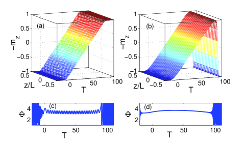
Figure 1: (Color online) The uniform autoresonant magnetization state. (a) -z-component of magnetization $-m_{z}$ versus slow time $T=\alpha^{1/2}\tau$; (c) phase mismatch $\Phi(0,T)=\phi-\phi_{d}$. In both panels $\lambda=0$ and $\varepsilon=3\times 10^{-3}$. Panels (b) and (d) are the same as (a) and (c), but $\lambda=3\times 10^{-3}$ and $\varepsilon=3\times 10^{-2}$.

We illustrate this effect in Fig. 1, showing the results of numerical simulations of the original system (1), assuming spatial periodicity of length $l=6$ and linearly chirped frequency $\Omega_{d}^{\prime}(\tau)=1-\alpha\tau$. The initial conditions $\theta=0.01\left|\cos(\kappa\xi)\right|$ ($\kappa=2\pi/l$) represented a small spatial perturbation for studying stability of the uniform state and we used parameters $\lambda=0$, $h_{0}=5$, $\varepsilon=3\times 10^{-3}$, and $\alpha=5\times 10^{-4}$ in Figs. 1a and 1c, while $\lambda=3\times 10^{-3}$ and $\varepsilon=3\times 10^{-2}$ in Figs. 1b and d. Our numerical scheme used an equivalent system of two coupled NLS-type equations based on the quantum two-level analog Feynman ; Lazar145 described in the Appendix. Figures 1a,b (without and with damping, respectively) show the evolution of $-m_{z}=-\cos\theta$ versus slow time $T=\alpha^{1/2}\tau$, which approximately follows the linear time dependence $\cos\theta\approx\Omega_{d}^{\prime}$ on time, while Figs. 1c,d represents the corresponding phase mismatch $\Phi(0,T)=\varphi(0,T)-\varphi_{d}(T)$, and illustrate the continuing azimuthal phase-locking in the system at $\Phi\approx\pi$. Note that the uniform solution in this case is stable with respect to spatial perturbations. The dissipation changes the threshold condition for entering the autoresonant uniform state Lazar94 ; Lazar145 , has some effect on the phase mismatch (compare Figs. 1c and d) and leads to the collapse of the solution to the initial equilibrium after dephasing. Nevertheless, in the phase-locked stage the autoresonant uniform solutions are similar with and without damping and remains stable with respect to spatial perturbations. In contrast to the example in Fig. 1, one observes a spatial instability of the autoresonant uniform state in Figs. 2a and b, showing the numerical simulations with the same parameters as in Fig. 1a and b, but $l=8$ instead of $6$. One can see the destruction of the uniform state in Fig. 2 and formation of a complex spatio-temporal structure of $m_{z}(\xi/l,T)$ starting $T\approx 21$ in Fig. 1a and somewhat earlier in Fig. 1b. These results can be explained by a perturbation theory as described below.

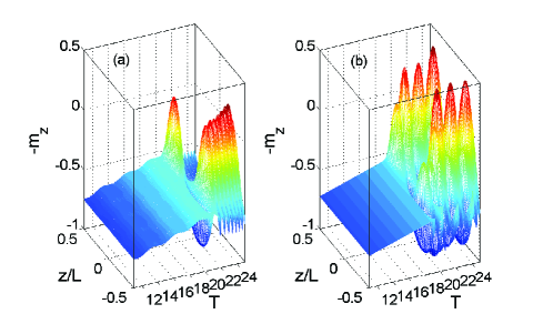
Figure 2: (Color online) The instability of the uniform magnetization state. The parameters of the simulations in (a) and (b) are the same as in Figs. 1a and 1b respectively, but $\kappa=2\pi/L<1$. A complex spatio-temporal magnetization profile develops beyond the point of instability.

We neglect damping for simplicity, freeze the time at $\tau=\tau_{0}$ and set $\Phi=\pi+\delta\Phi$ and $\theta=\theta_{0}+\delta\theta$, where $\theta_{0}$ satisfies

$$\cos\theta_{0}-\Omega_{d}^{\prime}(\tau_{0})+\varepsilon\cot\theta_{0}=0.$$ (12)

Then, for small perturbations $\delta\Phi$ and $\delta\theta$ of frequency $\nu$ and wave vector $\kappa$, Eqs. (3) and (4) become

$$-i\nu\delta\theta = -(\kappa^{2}\sin\theta_{0}-\varepsilon)\delta\Phi,$$ (13)

$$-i\nu\delta\Phi = \left(-\sin\theta_{0}+\frac{\kappa^{2}}{\sin\theta_{0}}-\frac{\varepsilon}{\sin^{2}\theta_{0}}\right)\delta\theta,$$

yielding

$$\nu^{2}=\frac{1}{\sin^{2}\theta_{0}}(\kappa^{2}\sin\theta_{0}-\varepsilon)\left(-\sin^{3}\theta_{0}+\kappa^{2}\sin\theta_{0}-\varepsilon\right).$$ (14)

One can see that for small $\varepsilon$, the uniform solution is stable with respect to spatial perturbations provided

$$\kappa>\sin\theta_{0}.$$ (15)

The examples in Figs. 1 ($\kappa=1.047$) and 2 ($\kappa=0.785$) are consistent with this result.

III III Transformation from spatially uniform solution to a standing wave

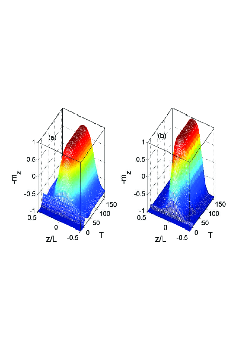
Figure 3: (Color online) The formation of autoresonant standing waves from the uniform magnetization state: (a) $\kappa=0.78$, (b) $\kappa=0.45$. The final waveform is reached as the driving frequency gradualy decreases and stays constant for $T>69$.

The formation of a uniform autoresonant solution $\cos\theta_{0}(\tau)\approx$ $\Omega_{d}^{\prime}(\tau)$ in the spatially periodic LLG problem was demonstrated above using a constant amplitude chirped frequency drive, yielding stable evolution provided the inequality (15) is satisfied (see Fig. 1). If during the evolution, this inequality is violated, the spatial instability develops (see Fig. 2). However, one can avoid the instability and transform the uniform autoresonant solution into an autoresonant standing wave by adding a simple spatial modulation of the driving amplitude, i.e., uses $\varepsilon=\varepsilon_{0}+\varepsilon_{1}\cos(\kappa\xi)$. We illustrate this phenomenon via simulations in Fig. 3, where we use parameters $\alpha=5\times 10^{-4}$ and $\lambda=0$, but, in the driving term, apply a modulated drive with $\varepsilon_{1}=\varepsilon_{0}=3\times 10^{-3}$ and switch on $\varepsilon_{1}$ at $\tau=0$. The chirped driving frequency in this numerical example is of form $\Omega_{d}^{\prime}=1-\Delta\Omega\sin(\alpha\tau/\Delta\Omega)$ for $\tau<\pi\Delta\Omega/2\alpha$ and $\Omega_{d}^{\prime}=1-\Delta\Omega$ for $\tau>\pi\Delta\Omega/2\alpha$, and we use $\Delta\Omega=0.98$. Thus, as in previous illustrations, the frequency passes the resonance at $\tau=0$ having chirp rate $\alpha$, but then gradually decreases reaching a constant. Figure 3a (where we use $l=8$) shows that the addition of the spatial modulation of the driving amplitudes prevents the spatial instability and leads to the emergence of a growing amplitude standing wave solution. Figure 3b (where $l=13)$ shows a similar dynamics, yielding formation of larger amplitude standing wave, which starts earlier, at $T\approx 5$ (we again use the slow time $T=\alpha^{1/2}\tau$ in this and the following figures). The excited standing wave is fully controlled by the variation of the driving frequency and precesses azimuthaly with the angular velocity of the driving phase (due to the continuing phase locking of $\Phi\approx\pi$). Furthermore, the magnetization waveform is spatially locked to the driving perturbation, while the wave amplitude and form is controlled by the instantaneous frequency of the drive. Importantly, as $l$ increases, the maximum and the minimum of the final solution for $m_{z}$ become near $+1$ and $-1$, respectively. We have also verified numerically that this solution approaches the well known soliton form with exponentially falling tails [see Eq. (6.21) in Ref. Kosevich ]. We further illustrate the autoresonant control of the standing magnetization waves in Figs. 4a and 4c, where we show the results of simulations with all the parameters of Fig. 3b, but instead of saturating the driving frequency, allow it to vary according the same sinusoidal formula for an additional time interval $\pi\Delta\Omega/2\alpha<\tau<\pi\Delta\Omega/2\alpha$, so the frequency returns to its original value. Figures 4b and 4d show the results of similar simulations with the same parameters as in Figs. 4a and 4c, but $\varepsilon=10^{-2}$ and $\lambda=10^{-3}$. One observes the return of the magnetization to its initial uniform state, being continuously phase locked (see Fig. 4c and 4d) to the drive with or without dissipation.

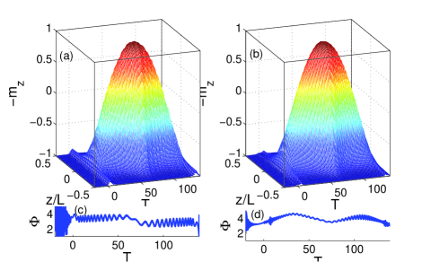
Figure 4: (Color online) The control of the phase-locked standing magnetization wave by varying the driving frequency. In (a) and (c) the parameters of the simulations are the same as in Fig. 3b, but after reaching its minimal value at $T=69$, the driving frequency increases back to the initial value, while the magnetization returns to the initial state. Panels (b) and (d) show $-m_{z}$ and phase mismatch $\Phi$, respectively versus slow time in the same case as (a) and (c), but $\lambda=10^{-3}$ and $\varepsilon=10^{-2}$.

The idea of the transformation from the uniform to standing wave solution by passage through the spatial instability originates from the similarity to the autoresonant excitations of standing waves of the driven-chirped nonlinear Schrodinger (NLS) equation Lazar82 :

$$i\psi_{\tau}+\psi_{\xi\xi}+\left|\psi\right|^{2}\psi+\varepsilon e^{-i\int\omega_{d}d\tau}=0.$$ (16)

If one writes $\psi=ae^{-i\phi}$ and separates the real and imaginary parts in (16), one arrives at the system

$$a_{\tau} = a\Phi_{\xi\xi}+2\Phi_{\xi}a_{\xi}-\varepsilon\sin\Phi,$$ (17)

$$\Phi_{\tau} = -\frac{a_{\xi\xi}}{a}+\Phi_{\xi}^{2}-a^{2}-\omega_{d}(t)-\frac{\varepsilon}{a}\cos\Phi.$$ (18)

where $\Phi=\phi-\int\omega_{d}d\tau$. Similarly to our ferromagnetic problem, the passage through the linear resonance in this system yields excitation of the uniform autoresonant NLS solution followed by transformation into autoresonant standing wave Lazar82 . One notices the structural similarity between this NLS system and LLG Eqs. (3) and (4), so we proceed to the theory for the magnetization case using the driven NLS ideas.

We assume that the time evolution in Eqs. (3) and (4) is slow and interpret the solutions at a given time $\tau$, as being a slightly perturbed solutions of the same system of equations, but with the time derivatives and the forcing terms set to zero, i.e.,

$$\Phi_{\xi\xi}\sin\theta+2\Phi_{\xi}\theta_{\xi}\cos\theta = 0,$$ (19)

$$\left(-\frac{1}{\sin\theta}\theta_{\xi\xi}+\Phi_{\xi}^{2}\cos\theta\right)-\Omega_{d}^{\prime}(\tau)+\cos\theta = 0.$$

We notice that this is a dynamical, two degrees of freedom problem ($\xi$ serving as ”time”) governed by Hamiltonian

$$H=\frac{1}{2}(\theta_{\xi}^{2}+\Phi_{\xi}^{2}\sin^{2}\theta)+V(\theta),$$ (20)

where

$$V(\theta)=-\Omega_{d}^{\prime}(\tau)\cos\theta+\frac{1}{4}\cos(2\theta).$$ (21)

This fixed $\tau$ problem is integrable since it conserves the canonical momentum $B=\Phi_{\xi}\sin^{2}\theta$ and energy

$$A=\frac{1}{2}\theta_{\xi}^{2}+V_{eff},$$ (22)

where $V_{eff}(\theta,\tau)=\frac{B^{2}}{2\sin^{2}\theta}+V(\theta)$. Next, we discuss oscillating solutions of this problem and introduce the conventional action-angle variables $(I,\Theta)$ and $(B,\Phi)$, where the first pair describes pure $\theta$ oscillations in the effective potential $V_{eff}$, while the second pair is associated with the dynamics of $\Phi$. If one returns to the original (time dependent and driven) system  (3) and (4), $A(\tau)$ and $B(\tau)$ become slow functions of time. We will present a theory describing these slow parameters via Whitham’s average variational principle Whitham in the next section and devote the remaining part of the current section to a simple qualitative picture of the dynamics.

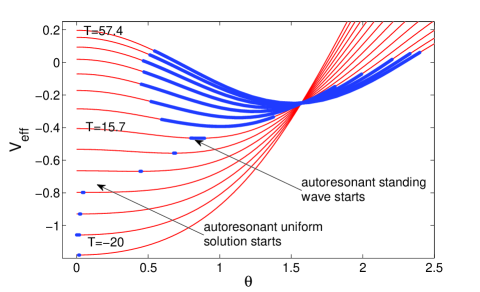
Figure 5: (Color online) The formation of the autoresonant standing wave modelled via dynamics of a quasi-particle in a slowly varying effective potential $V_{eff}$. $V_{eff}$ versus $\theta$ is shown for successive times (thin red lines) starting at $T=-20$. The thick blue lines show spatial oscillations of $\theta$ at these times, as obtained in simulations in Fig. 3a. The excitation proceeds as the quasi-particle remains at the bottom of the potential well continuously, corresponding to the flat solution. After passage through resonance with the spatial modulation of the driving amplitude, autoresonant oscillations of the quasi-particle in the effective potential are excited, describing the standing magnetization wave.

Our qualitative picture is based on the assumption of almost purely $\theta$ dynamics in the problem, i.e., setting $B\approx 0,$ which means a continuous phase locking $\Phi\approx\pi$, simplifying the effective potential to $V_{eff}\approx-\Omega_{d}^{\prime}(\tau)\cos\theta+\frac{1}{4}\cos(2\theta)$. As already discussed above, the phase locking at $\pi$ is guaranteed in the initial excitation stage via temporal autoresonance with constant amplitude $\varepsilon=\varepsilon_{0}$, chirped frequency perturbation. But now our driving amplitude $\varepsilon=\varepsilon_{0}+\varepsilon_{1}\cos(\kappa\xi)$ has two terms, where the first leads to excitation of the uniform autoresonant solution as discussed above, while the second term yields transition to the standing wave solution. Initially, $\theta$ is efficiently trapped at the minimum location $\theta_{m}$ of the potential well $V_{eff}$ given by $\cos\theta_{m}=\Omega_{d}^{\prime}(\tau).$ To $O(\varepsilon)$ this yields $\theta\approx\theta_{m}$, so this dynamics corresponds to the uniform autoresonant solution [see Eq. (12)]. The second term $\varepsilon_{1}\cos(\kappa\xi)$ in the driving has little effect on the evolution at this stage, until the spatial frequency $\kappa_{0}=\sqrt{\partial^{2}V_{eff}/\partial\theta_{m}^{2}}$ of oscillations of $\theta$ around $\theta_{m}$ passes the resonance with this driving term, i.e. when

$$\Omega_{d}^{\prime}(\tau)\cos\theta_{m}-\cos(2\theta_{m})\approx\sin^{2}\theta_{m}=\kappa^{2}.$$ (23)

But this is exactly the location of the instability of the uniform solution [see Eq. (15)] without the term $\varepsilon_{1}\cos(\kappa\xi)$ in the drive. The passage through the resonance with this new drive term excites growing amplitude oscillations of $\theta$ in the effective potential. After the passage, the oscillations of $\theta$ become autoresonant as the amplitude increases to preserve their spatial frequency near $\kappa$ continuously. These newly induced spatially phase-locked, growing amplitude oscillations of $\theta$ comprise the autoresonant standing wave solution. The amplitude of these oscillations  does not grow indefinitely. Indeed, when the potential $V_{eff}$ becomes shallower again as $\theta_{m}$ passes $\pi/2$ at $\Omega_{d}^{\prime}(\tau)=0$, the spatial resonance can not be sustained, and the autoresonance is expected to interrupt. We illustrate this dynamics in Fig. 5, showing the effective potential $V_{eff}$ (thin red lines) at $14$ successive values of slow time starting $T=-20$. The thick blue lines in the figure show the value of the potential at $\theta(\xi,T)$ at these times, as obtained in the simulations in the example in Fig. 3a.

IV IV Whitham’s averaged variational analysis

IV.1 Averaged Lagrangian density

The LLG problem governed by Eqs. (3) and (4) allows Lagrangian formulation with the Lagrangian density $L=L_{0}+L_{1}$ where

$$L_{0}(\theta,\theta_{\xi},\Phi_{\tau},\Phi_{\xi},\tau) = \frac{1}{2}(\theta_{\xi}^{2}+\Phi_{\xi}^{2}\sin^{2}\theta)+\Phi_{\tau}\cos\theta$$ (24)

$$+\Omega_{d}^{\prime}(\tau)\cos\theta-\frac{1}{4}\cos(2\theta)$$

and the perturbing part

$$L_{1}=-\varepsilon\sin\theta\cos\Phi.$$ (25)

For studying the slow autoresonant evolution in system (3) and (4), we use Whitham’s averaged Lagrangian approach. Following Lazar81 ; Lazar82 , describing a similar NLS problem, we seek solutions of form

$$\theta=\vartheta(\tau)+U(\Theta,\tau),\Phi=\upsilon(\tau)+V(\Theta,\tau),$$ (26)

where the explicit time dependence is slow, while $\Theta(\xi,\tau)$ is a fast variable and $U$ and $V$ are $2\pi$ periodic in $\Theta$. In addition, the frequencies $\Theta_{\tau}=-\Omega(\tau)$ and $\beta=\upsilon_{\tau}$ are slow functions of time and the wave vector $\Theta_{\xi}=\kappa=const$ ($\kappa=2\pi/l$, $l$ being the periodicity length in our problem). The Whitham’s averaging Whitham in this system proceeds from the unperturbed Lagrangian density $L_{0}$, where one freezes the slow time dependence at some $\tau$ and, using $\Phi_{\xi}=\kappa V_{\Theta}$, replaces $\Phi_{\tau}=\beta-\Omega V_{\Theta}=\beta-(\Omega/\kappa)\Phi_{\xi}$. This yields

$$L_{0} = \frac{1}{2}(U_{\xi}^{2}+\Phi_{\xi}^{2}\sin^{2}\theta)$$ (28)

$$+\left(\beta+\Omega_{d}^{\prime}-\frac{\Omega}{\kappa}\Phi_{\xi}\right)\cos\theta-\frac{1}{4}\cos(2\theta).$$

Recall that the explicit dependence on $U$ in (28) enters via $\theta=\vartheta+U$. This Lagrangian density describes a two degrees of freedom dynamical problem (for $U$ and $\Phi$), where $\xi$ plays the role of ”time”. In dealing with this problem we use Hamiltonian formulation. We define the usual canonical momenta

$$P^{U} = \partial L_{0}/\partial U_{\xi}=U_{\xi}$$ (29)

$$P^{\Phi} = \partial L_{0}/\partial\Phi_{\xi}=\Phi_{\xi}\sin^{2}\theta-\frac{\Omega}{\kappa}\cos\theta$$ (30)

and observe that $\Phi$ is a cyclic variable and therefore $P^{\Phi}=B$ is the integral of motion. We will unfreeze the slow time dependence later and $B(\tau)$ will becomes a slow function of time. The Lagrangian density $L_{0}$ yields the Hamiltonian in the time-frozen problem

$$H_{0}=P^{U}U_{\xi}+P^{\Phi}\Phi_{\xi}-L_{0}$$ (31)

and, after some algebra,

$$H_{0}=H_{0}^{\prime}(P^{\theta},\theta)+V_{1}(\theta,B,\Omega,\beta),$$ (32)

where

$$H_{0}^{\prime}(P^{U},U) = \frac{1}{2}\left(P^{U}\right){}^{2}+V(\theta)-V(\vartheta),$$ (33)

$$V(\theta) = -\Omega_{d}^{\prime}\cos\theta+\frac{1}{4}\cos(2\theta),$$ (34)

and

$$V_{1}(B,\Omega,\beta,\theta)=V(\vartheta)+\frac{\left(B+\frac{\Omega}{\kappa}\cos\theta\right)^{2}}{2\sin^{2}\theta}-\beta\cos\theta.$$

At this stage, we return to the full driven (still time-frozen) problem governed by the Hamiltonian

$$H=H_{0}^{\prime}(P^{U},U)+V_{1}-L_{1}$$ (35)

(recall that $L_{1}=-[\varepsilon_{0}+\varepsilon_{1}\cos(\kappa\xi)]\sin\theta\cos\Phi$) and make canonical transformation from $P^{U},U$ to the action-angle ($AA$) variables $I,\Theta$ of Hamiltonian $H_{0}^{\prime}$. The dynamics governed by this Hamiltonian conserves its energy $A=H_{0}^{\prime}$ and is periodic of period $2\pi$ in $\Theta$, and, at this stage, we identify $\Theta$ with the angle variable used in the definitions (26). The action variable in $H_{0}^{\prime}$ problem is

$$I=\frac{1}{2\pi}\oint P^{U}dU=\frac{1}{2\pi}\oint\sqrt{2[A-V(\theta)+V(\vartheta)]}dU,$$ (36)

were the time dependence enters both explicitly in $V$ and via $\vartheta$. Note that

$$\frac{\partial I}{\partial A}=\frac{1}{2\pi}\oint\frac{1}{\sqrt{2[A-V(\theta)+V(\vartheta)]}}dU=\frac{1}{\widetilde{\kappa}},$$ (37)

$\widetilde{\kappa}(\vartheta,A)$ being the (spatial) frequency of the oscillations of $U$ governed by $H_{0}^{\prime}$. Next, we write the full Lagrangian in our problem in terms of the new action angle variables

$$L=\frac{d\Theta}{d\xi}I-H=\kappa I-A-V_{1}(B,\Omega,\beta,\theta)+L_{1}(\theta,\xi,\tau),$$ (38)

where $\theta=\vartheta+U(I,\Theta,\tau)$ in $V_{1}$ and $L_{1}$, as the result of the canonical transformation. The Whitham’s averaged Lagrangian density $\Lambda$ is obtained by averaging $L$ in the time-frozen problem over one oscillation governed by $H_{0}^{\prime}$:

$$\Lambda=\frac{1}{2\pi}\int_{0}^{2\pi}Ld\Theta=\kappa I-A-\frac{1}{2\pi}\int_{0}^{2\pi}(V_{1}-L_{1})d\Theta.$$ (39)

To complete the averaging, we calculate two remaining components $\left\langle V_{1}\right\rangle=\frac{1}{2\pi}\int_{0}^{2\pi}V_{1}d\Theta$ and $\Lambda_{1}=\frac{1}{2\pi}\int_{0}^{2\pi}L_{1}d\Theta$ in (39).

$$\left\langle V_{1}\right\rangle = V(\vartheta)+\frac{1}{2\pi}\int_{0}^{2\pi}\left[\frac{\left(B+\frac{\Omega}{\kappa}\cos\theta\right)^{2}}{2\sin^{2}\theta}-\beta\cos\theta\right]d\Theta$$ (40)

$$= V(\vartheta)+I_{1}\frac{B^{2}}{2}+I_{2}\frac{B\Omega}{\kappa}+I_{3}\frac{\Omega^{2}}{2\kappa^{2}}-\beta I_{4},$$

where $I_{1}=\left\langle\frac{1}{\sin^{2}\theta}\right\rangle,I_{2}=\left\langle\frac{\cos\theta}{\sin^{2}\theta}\right\rangle,I_{3}=\left\langle\frac{\cos^{2}\theta}{\sin^{2}\theta}\right\rangle,I_{4}=\left\langle\cos\theta\right\rangle$ and the averages $\left\langle...\right\rangle$ are defined as

$$\left\langle...\right\rangle=\frac{1}{2\pi}\int_{0}^{2\pi}(...)d\Theta=\frac{\kappa}{2\pi}\oint\frac{(...)}{\sqrt{2[A-V(\theta)+V(\vartheta)]}}dU.$$ (41)

Finally, we calculate the averaged driving part of the Lagrangian density (recall that $\theta=\vartheta+U$ and $\Phi=\upsilon+V$)

$$\Lambda_{1}=-\frac{1}{2\pi}\int_{0}^{2\pi}\left[\varepsilon_{0}+\varepsilon_{1}\cos(\kappa\xi)\right]\sin(\vartheta+U)\cos(\upsilon+V)d\Theta.$$ (42)

Here, we limit evaluation of this averaged object to small spatial oscillations of $\theta$ around $\vartheta$, write $U\approx a(I)\cos\Theta$ and replace $\sin(\vartheta+U)\approx\sin\vartheta+a(I)\cos\vartheta\cos\Theta$. Furthermore, we will also assume that $V$ is sufficiently small to replace $\cos(\upsilon+V)\approx\cos\upsilon$. Finally, assuming a continuous approximate double resonance in the problem, i.e. $\upsilon(\tau)-\pi=\upsilon^{\prime}\approx 0$ and $\Theta-\kappa\xi-\pi=\mu(\tau)\approx 0$ (initial phase locking of $\upsilon$ at $\pi$ was shown in the uniform autoresonant solution stage), after averaging

$$\Lambda_{1}\approx(\varepsilon_{0}\sin\vartheta-\frac{\varepsilon_{1}}{2}a(I)\cos\vartheta\cos\mu)\cos\upsilon^{\prime}.$$ (43)

Therefore, our final averaged Lagrangian becomes

$$\Lambda = \kappa I-A-V(\vartheta)-\frac{I_{1}B^{2}}{2}-\frac{I_{2}B\Omega}{\kappa}-\frac{I_{3}\Omega^{2}}{2\kappa^{2}}+I_{4}\beta$$ (44)

$$+\left[\varepsilon_{0}\sin\vartheta-\frac{\varepsilon_{1}}{2}a(I)\cos\vartheta\cos\mu\right]\cos\upsilon^{\prime}.$$

We discuss the slow evolution of the full driven system next. Following Whitham, this evolution is obtained by unfreezing the time and taking variations of $\Lambda$ with respect to all dependent variables $A,\vartheta,B,\Theta$ and $\upsilon$. Obviously, only slow objects enter the averaged Lagrangian density.

IV.2 Evolution equations and stability analysis

At this stage, we write variational evolution equations. The variation of $\Lambda$ with respect to $B$ yields

$$\frac{d\mu}{d\tau}=-\Omega=\frac{\kappa I_{1}}{I_{2}}B,$$ (45)

and the variation with respect to $\Theta$ and use of (45) results in

$$\frac{d}{d\tau}\left[\left(I_{2}^{2}-I_{1}I_{3}\right)\frac{B}{\kappa I_{2}}\right]\approx\frac{\varepsilon_{1}}{2}a\cos\vartheta\sin\mu.$$ (46)

Similarly, the variation with respect to $A$ and $\upsilon$ gives

$$I_{4A}\frac{d\upsilon^{\prime}}{d\tau} = 1-\frac{\kappa}{\widetilde{\kappa}}+B^{2}\left(\frac{I_{1A}}{2}-\frac{I_{2A}I_{1}}{I_{2}}+\frac{I_{3A}I_{1}^{2}}{2I_{2}^{2}}\right)$$

$$+\frac{\varepsilon_{1}}{2}a_{A}\cos\vartheta\cos\mu\cos\upsilon^{\prime}$$

and

$$\frac{dI_{4}}{d\tau}\approx-(\varepsilon_{0}\sin\vartheta-\frac{\varepsilon_{1}}{2}a\cos\vartheta\cos\mu)\sin\upsilon^{\prime}$$ (48)

Finally, the variation with respect to $\vartheta$ yields

$$I_{4\vartheta}\frac{d\upsilon^{\prime}}{d\tau} = \frac{\partial V(\vartheta)}{\partial\vartheta}-\kappa\frac{\partial I}{\partial\vartheta}+B^{2}\left(\frac{I_{1\vartheta}}{2}-\frac{I_{2\vartheta}I_{1}}{I_{2}}+\frac{I_{3\vartheta}I_{1}^{2}}{2I_{2}^{2}}\right)$$ (49)

$$-(\varepsilon_{0}\cos\vartheta+\frac{\varepsilon_{1}}{2}a\sin\vartheta\cos\mu)\cos\upsilon^{\prime}.$$

Equations (45)-(49) comprise a complete set of slow evolution equations for $A,B,\mu,\upsilon^{\prime}$ and $\vartheta$. The solution of these equations proceeds by defining a quasi-steady state $B_{0}=\mu_{0}=$ $\upsilon_{0}^{\prime}=0$, $\vartheta=\vartheta_{0}$ and $A_{0}$ given by

$$\left(V_{\vartheta}-\kappa I_{\vartheta}\right)_{A_{0},\vartheta_{0}}-\varepsilon_{0}\cos\vartheta_{0}-\frac{\varepsilon_{1}}{2}a\sin\vartheta_{0}=0,$$ (50)

$$G(A_{0},\vartheta_{0})=\left(1-\frac{\kappa}{\widetilde{\kappa}}+\frac{\varepsilon_{1}}{2}a_{A}\cos\vartheta_{0}\right)_{A_{0},\vartheta_{0}}=0,$$ (51)

Note that in the case $\varepsilon_{1}=0$ and small $A$, Eq. (50) nearly coincides with Eq. (12) describing the autoresonant uniform solution. Furthermore, for small $A,$ to $O(\varepsilon)$, Eq. (50) yields $V_{\vartheta_{0}}\approx 0$, i.e. $\vartheta_{0}$ remains near the location of the minimum of $V(\theta)$ given by $\cos\vartheta_{0}\approx\Omega_{d}^{\prime}$, as was suggested in the qualitative model in Sec. IV and seen in simulations. On the other hand, Eq. (51) clarifies the phase locking at $\mu\approx 0$ as $\widetilde{\kappa}$ approaches the resonance $\widetilde{\kappa}=\kappa$ from below. For small perturbations $\delta A,\delta B,\delta\mu,\delta\upsilon^{\prime}$ and $\delta\vartheta$ of the quasi-steady state, we use $I\approx\delta A/\widetilde{\kappa}\approx\delta A/\sin\vartheta$ to get the lowest order (linear) set of equations

$$\frac{d\delta\mu}{d\tau} = \frac{\kappa I_{1}}{I_{2}}\delta B,$$ (52)

$$\frac{d\delta B}{d\tau} = -\frac{\kappa\varepsilon_{1}aI_{2}\cos\vartheta}{2(I_{1}I_{3}-I_{2}^{2})}\delta\mu,$$ (53)

$$I_{4A}\frac{d\delta\upsilon^{\prime}}{d\tau} = G_{\vartheta}\delta\vartheta+G_{A}\delta A,$$ (54)

$$I_{4A}\frac{d\delta A}{d\tau}+I_{4\vartheta}\frac{d\delta\vartheta}{d\tau} = -(\varepsilon_{0}\sin\vartheta-\frac{\varepsilon_{1}}{2}a\cos\vartheta)\delta\upsilon^{\prime},$$ (55)

$$I_{4\vartheta}\frac{d\delta\upsilon^{\prime}}{d\tau} = V_{\vartheta\vartheta}\delta\vartheta-\kappa R\delta A$$ (56)

where we use $\widetilde{\kappa}\approx\sin\vartheta$, so $R\approx\cos\vartheta/\sin^{2}\vartheta$ and all coefficients in (52) - (56) are viewed as constants evaluated at the quasi-steady state. Eqs. (52) and (53) yield

$$\frac{d^{2}\delta\mu}{d\tau^{2}}+\nu_{1}^{2}\delta\mu\approx 0,$$ (57)

while Eqs. (54)-(56) reduce to

$$\frac{d^{2}\delta\upsilon^{\prime}}{d\tau^{2}}+\nu_{2}^{2}\delta\upsilon^{\prime}\approx 0,$$ (58)

where the two frequencies satisfy

$$\nu_{1}^{2} = \frac{\varepsilon_{1}\kappa^{2}I_{1}a\cos\vartheta}{2(I_{1}I_{3}-I_{2}^{2})},$$

$$\nu_{2}^{2} = \frac{(\varepsilon_{0}\sin\vartheta-\frac{\varepsilon_{1}}{2}a\cos\vartheta)(G_{A}V_{\vartheta\vartheta}-\kappa RG_{\vartheta})}{I_{4A}(I_{4A}V_{\vartheta\vartheta}-\kappa RG_{\vartheta})+I_{4\vartheta}(G_{A}I_{4\vartheta}-G_{\vartheta}I_{4A})}.$$

A positiveness of $\nu_{1,2}^{2}$ guarantees stability of the (doubly) autoresonant ($\upsilon^{\prime}\approx 0$ and $\mu\approx 0$) evolution of the system. We observe that

$$I_{1}I_{3}-I_{2}^{2}\propto\left(\sum_{i}\frac{1}{s_{i}}\right)\left(\sum_{j}\frac{x_{j}^{2}}{s_{j}}\right)-\left(\sum_{i}\frac{x_{i}}{s_{i}}\right)^{2},$$

where $x_{i}=\cos\theta_{i}$ and $s_{i}=\sin^{2}\theta_{i}\sqrt{[A-V_{eff}(\theta_{i})]}$ . Then

$$I_{1}I_{3}-I_{2}^{2}\propto\sum_{i,j>i}\frac{(x_{i}-x_{j})^{2}}{s_{i}s_{j}},$$ (59)

so $\nu_{1}^{2}$ is positive for $\vartheta_{0}<\pi/2$. Then, since $B=\delta B$, and $\mu=\delta\mu$, they both remain small. Furthermore, for small excitations of $A$, to lowest order in $A,$ $\kappa=\sin\vartheta$, $G_{\vartheta}=\cos\vartheta/\sin\vartheta$, $G_{A}=(\frac{1}{\sin\vartheta}-\frac{3}{2\sin^{3}\vartheta})$, $I_{4\vartheta}=-\sin\vartheta$, $I_{4A}=\cos\vartheta/\sin^{2}\vartheta$. With these substitutions, one finds $\nu_{2}^{2}\approx\varepsilon_{0}\sin\vartheta-\frac{\varepsilon_{1}}{2}a\cos\vartheta$. Then condition $\varepsilon_{0}\sin\vartheta-\frac{\varepsilon_{1}}{2}a\cos\vartheta>0$ guarantees the stability of the autoresonant evolution.

V V Spin torque driving

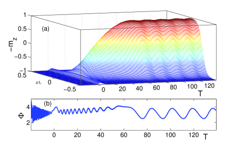
Figure 6: (Color online) Formation of the autoresonant standing magnetization wave by chirped frequency spin torque drive. The parameters in the simulations are the same as in Fig. 3b for the AC drive. Panels (a) and (b) show $-m_{z}$ and phase mismatch $\Phi(0,T)$, respectively versus $T$.

The excitation of the uniform solution and its transition to the autoresonant standing wave can be also achieved by using spin torque drive instead of the microwave drive used above (a related autoresonant problem for single domain nano-particles was studied in Ref. Lazar152 ). The effective magnetic field associated with the spin torque is

$$\mathbf{h}_{s}=\mathbf{m\times I}_{s},$$ (60)

where $\mathbf{I}_{s}$ is the dimensionless spin polarized current, which will be assumed of form $\mathbf{I}_{s}=2\varepsilon\sin\varphi_{d}\mathbf{e}_{x}$ in the following, yielding

$$\mathbf{h}_{s}=2\varepsilon(m_{z}\mathbf{e}_{y}-m_{y}\mathbf{e}_{z}).$$ (61)

The analog of system (3), (4) for this drive is

$$\theta_{\tau} = \Phi_{\xi\xi}\sin\theta+2\Phi_{\xi}\theta_{\xi}\cos\theta-\varepsilon\cos\theta\sin\Phi,$$ (62)

$$\Phi_{\tau} = \left(-\frac{1}{\sin\theta}\theta_{\xi\xi}+\Phi_{\xi}^{2}\cos\theta\right)-\Omega_{D}^{\prime}-\frac{\varepsilon\cos\Phi}{\sin\theta},$$ (63)

where $\Phi=\varphi-\varphi_{d}+\pi/2$.

Note that for small $\theta$ the last two equations are nearly the same as Eqs. (3), (4) for the microwave drive. One consequence of this is that the autoresonance threshold when passing the linear resonance is the same for both cases. Figure 6 illustrates the formation and control of the autoresonant standing wave via a spin torque drive in simulations using the parameters of Fig. 3b. One can see that the form of the excited solution in Figs. 3b and 6a are very similar. Despite this similarity, a complete Whitham’s-type theory of the spin torque driven problem is more complex than that for the microwave drive case, because the driving parts in Eqs. (62) and (63) do not allow Lagrangian description. Therefore, we leave this theory outside the scope of the present work.

VI VI Conclusions

In conclusion, we have studied the problem of autoresonant excitation and control of 1D standing magnetization waves in easy axis ferromagnetics in an external magnetic field  and driven by a weak circularly polarized, chirped frequency microwave field. We had modeled this problem by the spatially periodic time dependent LLG equation [see Eq. (1)]. We had discussed the excitation of the autoresonant solutions in this system via theory and compared the results with numerical simulations. The excitation proceeded as the driving frequency passed a resonance with the initially spatially uniform magnetization equilibrium in the direction of the easy axis (polar angle $\theta=0$), yielding a driven spatially uniform magnetization with the azimuthal angle $\varphi$ of the magnetization locked (and therefore controlled) by the phase of the microwave. This phase locking (autoresonance) reflects a continuous self-adjustment of $\theta$ [ see Eq. (11)], so that the resonance is preserved despite the variation of the driving frequency. It was shown that the condition for this autoresonant evolution is the driving amplitude $\varepsilon$ exceeding a threshold, which scales with the driving frequency chirp rate as $\varepsilon_{th}\sim\alpha^{3/4}$ [see Eq. (10)]. We had also shown that the uniform autoresonant magnetization state remained stable with respect to spatial perturbations if $\sin\theta<\kappa=2\pi/l$, $l$ being the periodicity length in the problem. In the case $2\pi/l>1$, the stable uniform state reached a complete magnetization inversion ($\theta\rightarrow\pi$)̇. In contrast, when $\theta$ increased during the autoresonant uniform state evolution and passed the point where $\sin\theta=2\pi/l$, the spatial instability developed, yielding a complex spatio-temporal magnetization wave form.

We had shown that if instead of a constant driving amplitude, one introduced a spatially modulated amplitude $\varepsilon_{0}+\varepsilon_{1}\cos(\kappa\xi)$, then, instead of the instability, a growing amplitude standing wave with the amplitude and form controlled by the frequency of the driving wave. This emerging autoresonant solution is doubly phase locked, i.e. its azimuthal angle $\varphi$ is locked to the phase of the driving wave, while $\theta$ performs slowly evolving growing amplitude nonlinear spatial oscillations in an effective potential, which are continuously phase-locked to the spatial frequency $\kappa$ of the modulation of the drive. Furthermore, as the periodicity length $l$ increases, the autoresonant standing wave approaches the well know soliton form [see Eq. (6.21) in Kosevich ]. The formation of the autoresonant standing is fully reversible and can be returned to its initial uniform ($\theta\approx 0$) state by simply reversing the variation of the driving frequency. In addition to suggesting a qualitative description of this autoresonant evolution (see Sec. III), we had developed a complete theory of the dynamics in the problem based on the Whitham’s averaged variational approach and studied modulational stability of the autoresonant solutions (see sec. IV). We had found numerically that a sufficiently weak dissipation does not affect the autoresonant evolution significantly. We had also discussed formation of autoresonant standing waves when replacing the microwave drive by a spatially modulated transverse spin torque driving and illustrated this possibility in numerical simulations. Developing a full Whitham’s type theory in this case and inclusion of dissipation and thermal fluctuations in the theory seem to be important goals for future research. Finally, it is known that the undriven, dissipationless LLG problem (1) is integrable Kosevich . This means that there exist many additional, so called multiphase solutions in this problem. Addressing the question of excitation and control of this multitude of solutions by chirped frequency perturbations seems to comprise another interesting goal for the future.

VII Appendix: Quantum two-level model

We perform our numerical simulations to lowest significant order in $\lambda$ and, therefore, approximate LLG Eq. (1) as

$$\frac{\partial\mathbf{m}}{\partial\tau}\approx\mathbf{h\times m+}\lambda\mathbf{m\times(h\times m)=h}^{\prime}\mathbf{\times m,}$$ (64)

where $\mathbf{h}^{\prime}=\mathbf{h}-\lambda\mathbf{h\times m.}$ Our numerical scheme for studying the evolution governed by Eq. (64) is based on the equivalent quantum two-level system (idea originated by Feynman Feynman , and recently used in studying magnetization inversion in single domain nano-particles Lazar145 ; Lazar152 ). We solve

$$i\frac{\partial A_{1}}{\partial\tau}=\frac{d_{0}}{2}A_{1}+dA_{2},$$ (65)

$$i\frac{dA_{2}}{\partial\tau}=-\frac{d_{0}}{2}A_{2}+d^{\ast}A_{1},$$ (66)

where $A_{1,2}=A_{1,2}(\xi,\tau)$ are the wave functions of a pair of coupled quantum levels and

$$d_{0} = h_{z}^{\prime},$$ (67)

$$d = \frac{(h_{x}^{\prime}-ih_{y}^{\prime})}{2}.$$ (68)

The magnetization $\mathbf{m}$ in $d_{0\text{ }}$and $d$ in Eqs. (65), (66) is related to $A_{1,2}$ via

$$m_{x} = A_{1}A_{2}^{\ast}+A_{1}^{\ast}A_{2}=2B_{1}B_{2}\cos\varphi,$$

$$m_{y} = i(A_{1}A_{2}^{\ast}-A_{1}^{\ast}A_{2})=2B_{1}B_{2}\sin\varphi,$$ (69)

$$m_{z} = \left|A_{1}\right|^{2}-\left|A_{2}\right|^{2}=B_{1}^{2}-B_{2}^{2},$$

where $A_{1,2}=B_{1,2}\exp(i\varphi_{1,2})$ and $\varphi=\varphi_{2}-\varphi_{1}$. Note that, as expected, the total population of our two level system remains constant, $\left|A_{1}\right|^{2}+\left|A_{2}\right|^{2}=|\mathbf{m|}=1$. Note also that $m_{\bot}=\sqrt{m_{x}^{2}+m_{y}^{2}}=2B_{1}B_{2}$, while $\varphi$ is the azimuthal rotation angle of the magnetization around $\xi$. Formally, the system (65), (66) comprises a set of two coupled NLS-type equations for wave functions $A_{1,2}$. The numerical approach to solving this system throughout this work used a standard pseudospectral method Canuto subject to given initial and periodic boundary conditions.

References

- (1) M.M. Scott, M.P. Kostylev, B.A. Kalinikos, C.E. Patton, Phys. Rev. B 71, 174440 (2005).
- (2) M. Wu, M. A. Kraemer, M.M. Scott, C.E. Patton, B.A. Kalinikos, Phys. Rev. B 70, 054402 (2004).
- (3) M. Wu, P.Krivosik, B.A. Kalinikos, C.E. Patton, Phys. Rev. Lett. 96, 227202 (2006).
- (4) M. Chen, M.A. Tsankov, J.M. Nash, C.E. Patton, Phys. Rev. Lett. 70, 1707 (1993).
- (5) A Scott, Nonlinear Science (Oxford University Press, New York, 1999) p. 279.
- (6) H.B. Braun, Adv. Phys. 61, 1 (2012).
- (7) G. Garbou, Math. Models. Meth. Appl. Sci. 11, 1529 (2001).
- (8) R.V. Kohn and V. Slastikov, Arch. Rat. Mech. Anal. 178, 227 (2005).
- (9) A.M. Kosevich, B.A. Ivanov, A.S. Kovalev, Phys. Rep. 194, 117 (1990).
- (10) H. -J. Mikeska, M. Steiner, Adv. Phys. 40, 191 (1991).
- (11) G. S. D. Beach, C. Nistor, C. Knutson, M. Tsoi, J. L. Erskine, Nature Mater. 4, 741 (2005).
- (12) A. Goussev, R.G. Lund, J.M. Robbins, V. Slastikov, C.Sonnenberg, Phys.Rev. B 88, 024425 (2013).
- (13) M. Negoita, T.J. Hayward, J.A. Miller, D. A. Allwood, J. Appl. Phys. 114, 013904 (2013).
- (14) M. Sitte, K. Everschor-Sitte, T. Valet, D.R. Rodrigues, J. Sinova, and Ar. Abanov, Phys. Rev. B 94, 064422 (2016).
- (15) W. Wang, Z. Zhang, R. A. Pepper, C. Mu, Y. Zhou, H. Fangohr, J. Phys.: Condens. Matter 30, 015801 (2018).
- (16) R. P. Cowburn, Nature (London) 448, 544 (2007).
- (17) L. Thomas, R. Moriya, C. Rettner, and S. S. P. Parkin, Science 330, 1810 (2010).
- (18) A.M. Kosevich, V.V. Gann, A.I.Zhukov, V.P. Voronov, Zh. Eksp. Teor. Fiz. 114, 735 (1998).
- (19) P.B. He, W.M. Liu, Phys. Rev. B 72, 064410 (2005).
- (20) Zai-Dong Li, Qiu-Yan Li, Lu Li, W.M. Liu, Phys.Rev. E 76, 026605 (2007).
- (21) E. M. McMillan, Phys. Rev. 68, 143 (1945).
- (22) V. I. Veksler, J. Phys. USSR 9, 153 (1945).
- (23) R. Malhotra, Nature (London) 365, 819 (1993).
- (24) L. Friedland, Astroph. J. Lett. 547, L75 (2001).
- (25) B. Meerson and L. Friedland, Phys. Rev. A 41, 5233 (1990).
- (26) H. Maeda, J. Nunkaew, and T. F. Gallagher, Phys. Rev. A 75, 053417 (2007).
- (27) J. Fajans, E. Gilson, and L. Friedland, Phys. Plasmas 6, 4497 (1999).
- (28) G. Klughertz, P-A. Hervieux, and G. Manfredi, J. Phys. D: Appl. Phys. 47, 345004 (2014).
- (29) G. Klughertz, L. Friedland, P-A. Hervieux, and G. Manfredi, Phys. Rev. B 91, 104433 (2015).
- (30) G. Klughertz, L. Friedland, P-A. Hervieux, and G. Manfredi, J. Phys. D 50, 415002 (2017).
- (31) L. Friedland, A. G. Shagalov, Phys. Rev. Lett. 81, 4357 (1998).
- (32) M.A. Borich, A. G. Shagalov, L. Friedland, Phys. Rev. E 91, 012913 (2015).
- (33) L. Friedland, A. G. Shagalov, Phys. Rev. E 71, 036206 (2005).
- (34) S. V. Batalov, A. G. Shagalov, Phys. Metals and Metallog. 109, 3 (2010).
- (35) S. V. Batalov, A. G. Shagalov, Phys.Rev. E 84 016603 (2011).
- (36) G. B. Whitham, Linear and Nonlinear Waves (Wiley, New York, 1974).
- (37) L. Friedland, Scholarpedia 4, 5473 (2009).
- (38) R. Feynman, F. L. Vernon, and R. W. Hellwarth, J. Appl. Phys. 28, 49 (1957).
- (39) J. Fajans, E. Gilson, and L. Friedland, Phys. Plasmas 8, 423 (2001).
- (40) L. Friedland, Phys. Rev. E 58, 3865 (1998).
- (41) C. Canuto, M. Y. Hussaini, A. Quarteroni, and T. A. Zang, Spectral Methods in Fluid Dynamics (Springer-Verlag, New York, 1988).