Peer Methods for the Solution of Large-Scale Differential Matrix Equations

Abstract

We consider the application of implicit and linearly implicit (Rosenbrock-type) peer methods to matrix-valued ordinary differential equations. In particular the differential Riccati equation (DRE) is investigated. For the Rosenbrock-type schemes, a reformulation capable of avoiding a number of Jacobian applications is developed that, in the autonomous case, reduces the computational complexity of the algorithms. Dealing with large-scale problems, an efficient implementation based on low-rank symmetric indefinite factorizations is presented. The performance of both peer approaches up to order 4 is compared to existing implicit time integration schemes for matrix-valued differential equations.

Author’s addresses:
Peter Benner
Max Planck Institute for Dynamics of Complex Technical Systems,
Computational Methods in Systems and Control Theory,
D-39106 Magdeburg, Germany,
and
Technische Universität Chemnitz,
Faculty of Mathematics, Mathematics in Industry and Technology
D-09126 Chemnitz, Germany
benner@mpi-magdeburg.mpg.de
Norman Lang
Technische Universität Chemnitz,
Faculty of Mathematics, Mathematics in Industry and Technology
D-09126 Chemnitz, Germany
norman.lang@mathematik.tu-chemnitz.de

1 Introduction

Differential matrix equations are of major importance in many fields like optimal control and model reduction of linear dynamical systems, see, e.g., [36, 1] and [49, 57], respectively. In that context, the most common differential matrix equations are the differential Riccati and Lyapunov equations (DREs/DLEs), where the latter can be considered as a special case of the Riccati equation. Therefore, as an illustrating example, in this article, we consider the numerical solution of the time-varying DRE

$$\begin{aligned} \dot{X}(t)&=A(t)^{T}X(t)+X(t)A(t)-X(t)S(t)X(t)+W(t)=:\mathcal{R}(t,X),\\ X(t_{0})&=X_{0},\end{aligned}$$ (1)

where $t\in[t_{0},t_{f}]$, $X(t)\in\mathbb{R}^{n\times n}$ is the sought for solution to Equation (1) and $A(t)$, $W(t)$, $S(t)\in\mathbb{R}^{n\times n}$ are given matrix-valued functions and the matrix $X_{0}\in\mathbb{R}^{n\times n}$ denotes the initial value with $n$ being the problem dimension. The differential Lyapunov equation results if we set $S(t)\equiv 0$. Provided that the matrices $A,W,S$ are piecewise continuous and locally bounded, from [1, Theorem 4.1.6] we have that a solution to Equation (1) exists and further is unique.

The DRE is one of the most deeply studied nonlinear matrix differential equations due to its importance in optimal control, optimal filtering, $\mathbf{H}_{\infty}$-control of linear-time varying systems, differential games and many more (see, e.g., [1, 22, 23, 42]). Over the last four decades many solution strategies have been presented, see, e.g., [15, 30, 35, 21, 25, 37]. Most of these methods are only applicable to small-scale systems, i.e., systems with a rather small number $n$ of unknowns. Others, suitable for the application to large-scale problems have to deal with numerical difficulties like, e.g., instability, see [38, Section 4.1] for a detailed overview. Due to the fact that in many control applications fast and slow modes are present, the DRE (1) is usually fairly stiff. For that reason, the numerical solution based on matrix versions of classical implicit time integration schemes, such as the BDF, Rosenbrock methods, and the Midpoint and Trapezoidal rules [16, 7, 38, 8, 9] has become a popular tool for the solution of (1). Recently, also splitting methods [20, 52, 53] and a structure preserving solution method for large-scale DREs [28], using Krylov subspace methods, were proposed. Note that “unrolling” the matrix differential equation into a standard (vector-valued) ordinary differential equation (ODE) is usually infeasible due to the resulting complexity - the ODE would then be posed in $\mathbb{R}^{n^{2}\times n^{2}}$.

In the field of implicit time integration methods, linear multistep and one-step methods, such as e.g., the BDF and the Rosenbrock methods, respectively, have been known for many decades and in addition have proven their effectiveness over the years for a wide range of problems. These two traditional classes of time integration methods have been studied separately until recently. As a unifying framework for stability, consistency and convergence analysis for a wide variety of methods, also containing the aforementioned classes, in [12] the general linear methods (GLMs) were introduced. Detailed explanations on GLMs are given in the surveys [13, 14]. Most of the classical methods contain a number of solution variables $X_{k+1,j}$ and in addition compute a separate number of auxiliary variables related to function evaluations $F(\tilde{t}_{k},\tilde{X}_{k})$ at $t_{k}\leq\tilde{t}_{k}\leq t_{k+1}$, $\tilde{X}_{k}\approx X(\tilde{t}_{k})$ that are designated to improve the accuracy and stability properties of the approximate solutions. In particular, usually only one solution variable for the approximation of the solution in each time interval is employed. Moreover, for different time intervals, as, e.g., for variable time step sizes, these solution variables may have distinguished accuracy and stability properties. Due to that e.g., the Rosenbrock methods often suffer from order reduction. Now, the idea of the so-called peer methods is to define an integration scheme that only contains peer variables, each representing an approximation to the exact solution of (1) at different time locations that share the same accuracy and stability properties.

For all the above mentioned implicit solution methods, including the peer methods to be presented, it turns out that the main ingredient for the solution of the DRE (1) is to solve a number of either algebraic Riccati or Lyapunov equations (AREs/ALEs) in each time step. Dealing with large-scale systems, the simple application of the implicit integration methods leads to an enormous computational effort and storage amount in the sense that the solution to the DRE (1) is a dense square matrix of dimension $n$ being computed at each point of the discrete time set. However, in practice it is often observed that the singular values of the solution of the ALEs occurring in the innermost iteration of the solution methods decay rapidly to zero, see, e.g., [2, 18, 40, 56]. Thus, the solution is of low numerical rank, meaning it can be well approximated by products of low-rank matrices. Based on this observation, modern and efficient algorithms rely on low-rank based solution algorithms. In [38, 8, 9] classical implicit time integration methods, originally developed for standard scalar and vector-valued ODEs, exploiting the low-rank phenomena were presented. Therein a factorization $X=ZZ^{T}$ with $Z\in\mathbb{R}^{n\times k}$, $k\ll n$, is employed in order to efficiently solve large-scale DREs. This decomposition will be referred to as a low-rank Cholesky-type factorization (LRCF) in the remainder. In [33, 34], it has be shown that for integration methods of order $\geq 2$, the right hand sides of the ALEs to be solved become indefinite and thus the LRCF involves complex data and therefore requires complex arithmetic and storage. Moreover, therein a low-rank symmetric indefinite factorization (LRSIF) of the form $X=LDL^{T}$, $L\in\mathbb{R}^{n\times k},~{}D\in\mathbb{R}^{k\times k}$, $k\ll n$, of the solution, was introduced in order to avoid complex data.

The paper is organized as follows. In Section 2, the implicit and linearly implicit Rosenbrock-type peer methods are introduced for the application to the matrix-valued differential Riccati equation. Efficient numerical algorithms based on the low-rank symmetric indefinite factorization for both peer approaches are presented in Section 3. In Section 4, the performance of the new peer solution methods up to order 4 is compared to the existing implicit integration schemes of similar orders. A conclusion is given in Section 5.

2 Peer Methods

The class of peer methods first appeared in [45] in terms of linearly implicit integration schemes with peer variables, suitable for parallel computations by only using information from the previous time interval. A number of specific peer schemes and applications are presented in, e.g., [43, 44, 46, 47]. Further, for a recent detailed overview see [54, Chapters 5,10].

2.1 General Implicit Peer Methods

A general (one-step) implicit peer method, applied to the matrix-valued initial value problem (1) reads

$$X_{k,i}= \sum_{j=1}^{s}b_{i,j}X_{k-1,j}+\tau_{k}\sum_{j=1}^{i}g_{i,j}\mathcal{R}(t_{k,j},X_{k,j}).$$ (2)

Here, $s$ is the number of stages and

$$t_{k,j}=t_{k}+c_{j}\tau_{k},$$ (3)

where the variables $c_{j},~{}j=1,\dots,s$, with $c_{s}=1,~{}t_{k,s}=t_{k+1}$, define the locations of the peer variables $X_{k,i},~{}i=1,\dots,s$, for the time step $t_{k}\rightarrow t_{k+1}$. In general, $c_{j}<0$ for some $j$ will also be allowed. Furthermore, the peer variables $X_{k,i}$ represent the solution approximations of (1) at the time locations $t_{k,i}$, i.e, $X_{k,i}\approx X(t_{k,i})=X(t_{k}+c_{i}\tau_{k})$. From $c_{s}=1$, the solution $X_{k}$ at time $t_{k}$ is given by $X_{k-1,s}$. The variables $b_{i,j}$ and $g_{i,j}$ are the determining coefficients of the method.

The convergence order of these methods is restricted to $s-1$. Thus, additionally using function values from the previous time interval, two-step peer methods of order $s$ can be constructed. Under special conditions even a superconvergent subclass of the implicit peer methods with convergence order $s+1$ can be found. Details on the convergence analysis are given in, e.g., [51] and the references therein. The corresponding two-step scheme becomes

$$X_{k,i}= \sum_{j=1}^{s}b_{i,j}X_{k-1,j}+\tau_{k}\sum_{j=1}^{s}a_{i,j}\mathcal{R}(t_{k-1,j},X_{k-1,j})+\tau_{k}\sum_{j=1}^{i}g_{i,j}\mathcal{R}(t_{k,j},X_{k,j})$$ (4)

with additional coefficients $a_{i,j}$.

Note that, given from the order conditions, the coefficients will in general depend on the step size ratio $\tau_{k}/\tau_{k-1}$ of two consecutive time steps. Moreover, the computation of the coefficients is based on highly sophisticated optimization processes. Therefore, for details on the order conditions and the computation of the associated coefficients, we refer to [51] and the references therein. Further, note that the scheme (2) can easily be recovered from (4) by setting $a_{i,j}=0$ and therefore in the remainder the statements restrict to the more general class (4) of implicit (two-step) peer methods.

From the application of the peer scheme (4) to the DRE (1) with $F(t_{k,i},X_{k,i})=\mathcal{R}(t_{k,i},X_{k,i})$ one obtains

$$\tilde{A}_{k,i}^{T}X_{k,i}+X_{k,i}\tilde{A}_{k,i}-X_{k,i}\tilde{S}_{k,i}X_{k,i}+\tilde{W}_{k,i}=0,\qquad i=1,\dots,s,$$ (5)

that in fact is an algebraic Riccati equation. Here, the coefficient matrices are given by

$$\tilde{A}_{k,i} =\tau_{k}g_{i,i}A_{k,i}-\frac{1}{2}I,\quad\tilde{S}_{k,i}=\tau_{k}g_{i,i}S_{k,i},$$

$$\tilde{W}_{k,i} =\tau_{k}g_{i,i}W_{k,i}+\sum_{j=1}^{s}b_{i,j}X_{k-1,j}+\tau_{k}\sum_{j=1}^{s}a_{i,j}\mathcal{R}(t_{k-1,j},X_{k-1,j})+\tau_{k}\sum_{j=1}^{i-1}g_{i,j}\mathcal{R}(t_{k,j},X_{k,j}).$$

Moreover, we have $A_{k,i}=A(t_{k,i})$, $W_{k,i}=W(t_{k,i})$ and $S_{k,i}=S(t_{k,i})$ with $t_{k,i}$ from Equation (3). Note that, according to the number of peer variables to be computed, $s$ AREs have to be solved at every time step $t_{k}\to t_{k+1}$ of the method.

In comparison, the BDF methods, as well as the Midpoint and Trapezoidal rules, require the solution of only one ARE at every time step, see e.g., [38, 34, 32]. That is, directly solving the occurring algebraic Riccati equations, the expected computational effort of the peer methods is in general $s$-times higher than that of the other implicit methods. Still, from the fact that $s$ peer variables with the same accuracy and stability properties are computed within every time interval, the peer methods allow us to use larger step sizes in order to achieve a comparable accuracy. A comparison and detailed investigation is given in Section 4. Note that analogously to the DRE case, the peer method can be applied to differential Lyapunov equations or any other differential matrix equation. The application to differential Lyapunov equations is presented in [32].

For solving the AREs, in general, any solution method suitable for sparse large-scale problems can be applied. A detailed overview can, e.g., be found in [11, 50]. In this contribution, Newton’s method is going to be used in order to find a solution to the AREs (5) arising within the peer scheme (4). Following [26, 31], Newton’s method applied to the AREs (5) results in the solution of an algebraic Lyapunov equation

$${{}\hat{A}_{k,i}^{(\ell)}}^{T}X_{k,i}^{(\ell)}+X_{k,i}^{(\ell)}\hat{A}_{k,i}^{(\ell)}=-\tilde{W}_{k,i}-X_{k,i}^{(\ell-1)}\tilde{S}_{k,i}X_{k,i}^{(\ell-1)}$$ (6)

with

$$\hat{A}_{k,i}^{(\ell)} =\tilde{A}_{k,i}-\tilde{S}_{k,i}X_{k,i}^{(\ell-1)}.$$

at each step $\ell$ of the Newton iteration and thus the solution of (1), using the implicit peer scheme (4) boils down to the solution of a sequence of ALEs at every time step of the integration scheme.

2.2 Rosenbrock-Type Peer Methods

2.2.1 Standard Representation

For the implicit peer methods applied to the DRE, a number of AREs has to be solved. In order to avoid the solution of these nonlinear matrix equations, we also consider linearly implicit peer methods in terms of the two-step Rosenbrock-type peer schemes

$$\begin{aligned} (I-\tau_{k}g_{i,i}J_{k})X_{k,i}=&\sum_{j=1}^{s}b_{i,j}X_{k-1,j}+\tau_{k}\sum_{j=1}^{s}a_{i,j}\left(F(t_{k-1,j},X_{k-1,j})-J_{k}X_{k-1,j}\right)\\ &+\tau_{k}J_{k}\sum_{j=1}^{i-1}g_{i,j}X_{k,j},\end{aligned}$$ (7)

introduced in [43]. As for the implicit schemes, here we consider methods with
$g_{1,1}=\dots=g_{s,s}=\gamma$. For the comprehensive derivation of coefficients $a_{i,j},~{}b_{i,j}$ and $g_{i,j}$ that result in stable schemes (7), for arbitrary step size ratios, we refer to [43, Section 3]. Expression $J_{k}$ denotes the Jacobian represented by the Fréchet derivative

$$J_{k}:=\frac{\partial\mathcal{R}}{\partial X}(t_{k},X_{k}):U\rightarrow(A_{k}-S_{k}X_{k})^{T}U+U(A_{k}-S_{k}X_{k}).$$ (8)

of $F$ at $(t_{k},X_{k})$. Now, replacing the Jacobian $J_{k}$ in (7) by (8), for the solution of the DRE, the procedure reads

$$\begin{aligned} \tilde{A}_{k,i}^{T}X_{k,i}&+X_{k,i}\tilde{A}_{k,i}=-\tilde{W}_{k,i}\quad i=1,\dots,s,\\ \tilde{W}_{k,i}=&\sum_{j=1}^{s}b_{i,j}X_{k-1,j}+\tau_{k}\sum_{j=1}^{s}a_{i,j}\left(\mathcal{R}(t_{k-1,j},X_{k-1,j})-(\hat{A}_{k}^{T}X_{k-1,j}+X_{k-1,j}\hat{A}_{k})\right)\\ &+\tau_{k}\sum_{j=1}^{i-1}g_{i,j}(\hat{A}_{k}^{T}X_{k,j}+X_{k,j}\hat{A}_{k})\end{aligned}$$ (9)

with the matrices $\hat{A}_{k}=A_{k}-S_{k}X_{k}$ and $\tilde{A}_{k,i}=\tau_{k}g_{i,i}\hat{A}_{k}-\frac{1}{2}I$.

2.2.2 Reformulation to avoid Jacobian applications

The Rosenbrock-type peer scheme (7) involves the solution of an ALE at each stage. The right hand sides of these ALEs particularly require the application of the Jacobian $J_{k}$ to the sums $\sum_{j=1}^{s}a_{i,j}X_{k-1,j}$ and $\sum_{j=1}^{i}g_{i,j}X_{k,j}$ of the previous and current solution approximations, respectively. In order to at least avoid the application of the Jacobians to the sum of new variables $X_{k,j}$, a reformulation, similar to what is standard for the classical Rosenbrock schemes, see, e.g., [19, Chapter IV.7], based on the variables

$$Y_{k,i}=\sum_{j=1}^{i}g_{i,j}X_{k,j},~{}i=1,\dots,s\Leftrightarrow\mathbf{Y}_{k}=(G\otimes I_{n})\mathbf{X}_{k}$$ (10)

can be stated. Here, $\mathbf{X}_{k}=(X_{k,i})_{i=1}^{s},~{}\mathbf{Y}_{k}=(Y_{k,i})_{i=1}^{s}\in\mathbb{R}^{sn\times n}$ and $\otimes$ denotes the Kronecker product. Provided that $g_{i,i}\neq 0,~{}\forall i$, the lower triangular matrix $G=(g_{i,j})$ is non-singular and the original variables $X_{k,i}$ can be recovered from the relation

$$\mathbf{X}_{k}=(G^{-1}\otimes I_{n})\mathbf{Y}_{k}\Leftrightarrow X_{k,i}=\sum_{j=1}^{i}\mathbf{g}_{i,j}Y_{k,j},~{}i=1,\dots,s$$ (11)

where $G^{-1}=(\mathbf{g}_{i,j})$ and $\mathbf{g}_{i,i}=\frac{1}{g_{i,i}}$. Then, from (11), we obtain

$$\begin{aligned} \sum_{j=1}^{s}\!a_{i,j}X_{k-1,j},i=1,\dots,s\Leftrightarrow\quad\!&~{}((a_{i,j})\otimes I)\mathbf{X}_{k}&\\ \!=&~{}((a_{i,j})\otimes I)(G^{-1}\!\otimes I)\mathbf{Y}_{k}&\\ \!=&~{}((a_{i,j})G^{-1}\otimes I)\mathbf{Y}_{k}&\!\!\!\!\!\Leftrightarrow\!\sum_{j=1}^{s}\!\mathbf{a}_{i,j}Y_{k-1,j},i=1,\dots,s\end{aligned}$$ (12)

with the coefficients

$$\begin{aligned} (\mathbf{a}_{i,j})=(a_{i,j})G^{-1}.\end{aligned}$$ (13)

and analogously, for the sum $\sum_{j=1}^{s}b_{i,j}X_{k-1,j}$, we have

$$\sum_{j=1}^{s}b_{i,j}X_{k-1,j}=\sum_{j=1}^{s}\mathbf{b}_{i,j}Y_{k-1,j},~{}i=1,\dots,s$$

with $(\mathbf{b}_{i,j})=(b_{i,j})G^{-1}$.

Now, inserting the auxiliary variables (10) into (7) and dividing the result by $\tau_{k}$, the linearly implicit scheme can be reformulated to

$$\begin{aligned} \left(\frac{1}{\tau_{k}g_{i,i}}I-J_{k}\right)Y_{k,i}=&~{}\sum_{j=1}^{s}\frac{\mathbf{b}_{i,j}}{\tau_{k}}Y_{k-1,j}+\sum_{j=1}^{s}a_{i,j}F(t_{k-1,j},\sum_{\ell=1}^{j}\mathbf{g}_{j,\ell}Y_{k-1,\ell})\\ &-J_{k}\sum_{j=1}^{s}\mathbf{a}_{i,j}Y_{k-1,j}-\sum_{j=1}^{i-1}\frac{\mathbf{g}_{i,j}}{\tau_{k}}Y_{k,j},\quad i=1,\dots,s.\end{aligned}$$ (14)

Again, replacing the Jacobian $J_{k}$ by (8), the modified Rosenbrock-type scheme, applied to the DRE, reads

$$\begin{aligned} \tilde{A}_{k,i}^{T}Y_{k,i}&+Y_{k,i}\tilde{A}_{k,i}=-\tilde{W}_{k,i},\\ \tilde{W}_{k,i}=&\sum_{j=1}^{s}\frac{\mathbf{b}_{i,j}}{\tau_{k}}Y_{k-1,j}+\sum_{j=1}^{s}a_{i,j}\mathcal{R}(t_{k-1,j},\sum_{\ell=1}^{j}\mathbf{g}_{j,\ell}Y_{k-1,\ell})\\ &-\sum_{j=1}^{s}\mathbf{a}_{i,j}(\hat{A}_{k}^{T}Y_{k-1,j}+Y_{k-1,j}\hat{A}_{k})-\sum_{j=1}^{i-1}\frac{\mathbf{g}_{i,j}}{\tau_{k}}Y_{k,j}\end{aligned}$$ (15)

with $\hat{A}_{k}$ from the original scheme and $\tilde{A}_{k,i}=\hat{A}_{k}-\frac{1}{2\tau_{k}g_{i,i}}I$.

Recall that the introduction of the auxiliary variables is capable of avoiding the application of the Jacobian $J_{k}$ to the sum of current stage variables. Still, the application remains for the sum of the previously determined peer variables. Moreover, in contrast to the classical Rosenbrock methods, the original solution approximations $X_{k,i}$ have to be reconstructed from the auxiliary variables by (11). That is, the reconstruction doubles the online storage amount for storing the solution approximations $X_{k,i}$ and the corresponding auxiliary variables $Y_{k,i},~{}i=1,\dots,s$, during the runtime of the integration method.

Summarizing, the linearly implicit peer methods result in the solution of $s$ ALEs, just like the classical Rosenbrock methods [38, 8], but directly compute the sought for solutions, instead of additional stage variables. Moreover, the additional stage variables from the classical Rosenbrock methods have a low stage order and therefore the integration procedures may suffer from order reduction. The computation of peer variables in the Rosenbrock-type peer scheme, sharing the same accuracy and stability properties, can overcome this well-known disadvantage [43] and again allows us to use larger time steps compared to the classical Rosenbrock methods.

3 Efficient Solution using Low-Rank Representations

As mentioned in the introduction, for small-scale problems, the implicit and Rosenbrock-type peer methods can directly be applied to the DRE, in general resulting in dense solutions. Thus, the explicit computation of the solution is not recommended for large-scale applications. Based on the observation that the solution to the ALEs in the innermost iteration often is of low numerical rank [2, 18, 40, 56], the literature provides a number of solution methods for large-scale ALEs based on low-rank versions of the alternating directions implicit (ADI) iteration and Krylov subspace methods. First developments considered a two-term LRCF of both ALE solution philosophies. Most recent improvements can, e.g., be found in [3, 4, 5, 29] and [24, 55, 17], respectively. Three-term LRSIF based formulations of these solution strategies have first been investigated for the more general case of Sylvester equations [6]. The specific application to ALEs, is extensively studied in [33, 34, 32]. The latter factorization is of major importance for the efficient solution of differential matrix equations. That is, the LRSIF allows to avoid complex data and arithmetic, arising within the classical low-rank two-term representation of the ALEs within the classical implicit integration schemes of order $\geq 2$. Note that for the implicit and Rosenbrock-type peer schemes complex data and arithmetic, in general, already occur for order $1$. The LRSIF has proven to show considerably better performance with respect to computational timings and storage amount in most applications. Note that there is some exceptions, see [34, 32] for details. Still, for the numerical experiments in Section 4, the algorithms used are restricted to the LRSIF based schemes. Moreover, we restrict to implementations using the ADI iteration for the solution of the innermost ALEs.

In order to exploit the low-rank phenomenon, a suitable low-rank representation of the right hand sides of the ALEs (6) and (9)/(15) within the implicit and linearly implicit Rosenbrock-type peer schemes, respectively, has to be found. In what follows, the LRSIF representations are presented. A detailed derivation of the LRCF based strategy and an extension to generalized DREs, also for the LRSIF approach, can be found in [32]. For the remainder, we define the mapping

$$H:\mathbb{R}^{n\times n}\rightarrow\mathbb{R}^{2n\times 2n},\quad H:I\mapsto H(I)=\begin{bmatrix}0&I\\ I&0\end{bmatrix}.$$

3.1 Low-Rank Implicit Peer Scheme

For the solution of the DRE (1) by implicit peer schemes, the main ingredient is to solve the algebraic Lyapunov equation

$$\begin{aligned} &{{}\hat{A}_{k,i}^{(\ell)}}^{T}X_{k,i}^{(\ell)}+X_{k,i}^{(\ell)}\hat{A}_{k,i}^{(\ell)}=-\tilde{W}_{k,i}-\tau_{k}g_{i,i}X_{k,i}^{(\ell-1)}S_{k,i}X_{k,i}^{(\ell-1)},\\ &\tilde{A}_{k,i}=\tau_{k}g_{i,i}A_{k,i}-\frac{1}{2}I,\quad\tilde{S}_{k,i}=\tau_{k}g_{i,i}S_{k,i},\\ &\hat{A}_{k,i}^{(\ell)}=\tilde{A}_{k,i}-\tilde{S}_{k,i}X_{k,i}^{(\ell-1)}-\frac{1}{2}I,\\ &\tilde{W}_{k,i}=\tau_{k}g_{i,i}W_{k,i}\!+\!\sum_{j=1}^{s}b_{i,j}X_{k-1,j}\!+\!\tau_{k}\!\sum_{j=1}^{s}\!a_{i,j}\mathcal{R}(t_{k-1,j},X_{k-1,j})\!+\!\tau_{k}\!\sum_{j=1}^{i-1}\!g_{i,j}\mathcal{R}(t_{k,j},X_{k,j})\end{aligned}$$ (16)

within every Newton step $\ell$ at each time step $t_{k}\to t_{k+1}$. Using low-rank versions of the ADI method, this requires the right hand side to be given in low-rank form as well. Provided $S_{k,i}$ and $W_{k,i}$ in the DRE (1) are given in the form

$$S_{k,i}=B_{k,i}B_{k,i}^{T},\quad W_{k,i}=C_{k,i}^{T}C_{k,i}$$

with $B_{k,i}\in\mathbb{R}^{n\times m}$ and $C_{k,i}\in\mathbb{R}^{q\times n}$, $m,q\ll n$, the right hand side of the ALE can also be written in factored form. Assume that the previous solution approximations $X_{k,j}$’s admit a decomposition of the form $X_{k,j}=L_{k,j}D_{k,j}L_{k,j}^{T}$ with $L_{k,j}\in\mathbb{R}^{n\times n_{L_{k,j}}},~{}D_{k,j}\in\mathbb{R}^{n_{L_{k,j}}\times n_{L_{k,j}}}$ such that the right hand side of (16) can be written in the form $-G_{k,i}^{(\ell)}S_{k,i}^{(\ell)}{{}G_{k,i}^{(\ell)}}^{T}$. In order to find such a symmetric indefinite decomposition of the entire right hand side, we first define a factorization for the Riccati operator $\mathcal{R}(.,.)$ in the form

$$\begin{aligned} \mathcal{R}(t_{k,j},\!X_{k,j})&\!=\!C_{k,j}^{T}C_{k,j}\!+\!A_{k,j}^{T}X_{k,j}\!+\!\!X_{k,j}A_{k,j}\!-\!\!X_{k,j}B_{k,j}B_{k,j}^{T}X_{k,j}\!=\!\mathcal{T}_{k,j}\mathcal{M}_{k,j}\mathcal{T}_{k,j}^{T},\\ \mathcal{T}_{k,j}&=\begin{bmatrix}C_{k,j}^{T},&A_{k,j}^{T}L_{k,j},&L_{k,j}\end{bmatrix}\in\mathbb{R}^{n\times(q+2n_{L_{k,j}})},\\ \mathcal{M}_{k,j}&=\begin{bmatrix}I_{q}&0&0\\ 0&0&D_{k,j}\\ 0&\quad D_{k,j}&\quad-D_{k,j}L_{k,j}^{T}B_{k,j}B_{k,j}^{T}L_{k,j}D_{k,j}\\ \end{bmatrix}\!\in\mathbb{R}^{(q+2n_{L_{k,j}})\times(q+2n_{L_{k,j}})}.\end{aligned}$$ (17)

For a more detailed derivation, we refer to [32]. Then, applying (17) to the right hand side

$$-\tilde{W}_{k,i} -\tau_{k}g_{i,i}X_{k,i}^{(\ell-1)}S_{k,i}X_{k,i}^{(\ell-1)},$$

of the ALE from Equation (16), the decomposition $G_{k,i}^{(\ell)}S_{k,i}^{(\ell)}{{}G_{k,i}^{(\ell)}}^{T}$ is given by the factors

$$G_{k,i}^{(\ell)}= \begin{bmatrix}C_{k,i}^{T},&L_{k-1,1},\dots,L_{k-1,s},&\mathcal{T}_{k-1,1},\dots,\mathcal{T}_{k-1,s},&\mathcal{T}_{k,1},\dots,\mathcal{T}_{k,i-1},&X_{k,i}^{(\ell-1)}B_{k,i}\end{bmatrix},$$

$$S_{k,i}^{(\ell)}= \operatorname{diag}\left(\tau_{k}g_{i,i}I_{q},~{}b_{i,1}D_{k-1,1},\dots,b_{i,s}D_{k-1,s},~{}\tau_{k}a_{i,1}\mathcal{M}_{k-1,1},\dots,\tau_{k}a_{i,s}\mathcal{M}_{k-1,s},\right.$$

$$\qquad\left.\tau_{k}g_{i,1}\mathcal{M}_{k,1},\dots,\tau_{k}g_{i,i-1}\mathcal{M}_{k,i-1},~{}\tau_{k}g_{i,i}I_{m}\right)$$

can be formulated and the desired factor $G_{k,i}^{(\ell)}$ is of column size

$$~{}q+\sum_{j=1}^{s}n_{L_{k-1,j}}+\sum_{j=1}^{s}(q+2n_{L_{k-1,j}})+\sum_{j=1}^{i-1}(q+2n_{L_{k,j}})+n_{L_{k,i}^{(\ell-1)}}$$

$$= ~{}(s+i)q+3\sum_{j=1}^{s}n_{L_{k-1,j}}+2\sum_{j=1}^{i-1}n_{L_{k,j}}+m.$$

For autonomous systems with constant system matrices, the inner ALE becomes

$${{}\hat{A}_{k,i}^{(\ell)}}^{T}X_{k,i}^{(\ell)}+X_{k,i}^{(\ell)}\hat{A}_{k,i}^{(\ell)}=-\tilde{W}_{k,i}-\tau_{k}g_{i,i}X_{k,i}^{(\ell-1)}BB^{T}X_{k,i}^{(\ell-1)}=-G_{k,i}^{(\ell)}S_{k,i}^{(\ell)}{{}G_{k,i}^{(\ell)}}^{T},$$

where $\hat{A}_{k,i}$ and the right hand side factors $G_{k,i}^{(\ell)},~{}S_{k,i}^{(\ell)}$ are given by

$$\hat{A}_{k,i}^{(\ell)} =\!\!\tau_{k}g_{i,i}(A-BB^{T}X_{k,i}^{(\ell-1)})-\frac{1}{2}I$$

$$G_{k,i}^{(\ell)} =\begin{bmatrix}C^{T},&L_{k-1,1},\dots,L_{k-1,s},&\mathcal{T}_{k-1,1},\dots,\mathcal{T}_{k-1,s},&\mathcal{T}_{k,1},\dots,\mathcal{T}_{k,i-1},&X_{k,i}^{(\ell-1)}B\end{bmatrix},$$

$$S_{k,i}^{(\ell)}= \operatorname{diag}\left(\tau_{k}(\sum_{j=1}^{s}a_{i,j}+\sum_{j=1}^{i}g_{i,j})I_{q},~{}b_{i,1}D_{k-1,1},\dots,b_{i,s}D_{k-1,s},\right.$$

$$~{}~{}\qquad\left.\tau_{k}a_{i,1}\mathcal{M}_{k-1,1},\dots,\tau_{k}a_{i,s}\mathcal{M}_{k-1,s},~{}\tau_{k}g_{i,1}\mathcal{M}_{k,1},\dots,\tau_{k}g_{i,i-1}\mathcal{M}_{k,i-1},~{}\tau_{k}g_{i,i}I_{m}\vphantom{\sum_{j=1}^{i}}\right)$$

where the factors $\mathcal{T}_{k,j},\mathcal{M}_{k,j}$ simplify to

$$\mathcal{T}_{k,j} =\begin{bmatrix}A^{T}L_{k,j},&L_{k,j}\end{bmatrix}\in\mathbb{R}^{n\times 2n_{L_{k,j}}},$$

$$\mathcal{M}_{k,j} =\begin{bmatrix}0&D_{k,j}\\ D_{k,j}&\quad-D_{k,j}L_{k,j}^{T}B_{k,j}B_{k,j}^{T}L_{k,j}D_{k,j}\\ \end{bmatrix}\in\mathbb{R}^{2n_{L_{k,j}}\times 2n_{L_{k,j}}}.$$

Then, the right hand side factor $G_{k,i}^{(\ell)}$ is of column size

$$q+3\sum_{j=1}^{s}n_{L_{k-1,j}}+2\sum_{j=1}^{i-1}n_{L_{k,j}}+m.$$

3.2 Low-Rank Rosenbrock-type Peer Scheme

3.2.1 Standard Rosenbrock-type Peer Representation

For the low-rank symmetric indefinite factorization based solution of a non-autonomous DRE (1), using the Rosenbrock-type peer method, we consider the ALE

$$\begin{aligned} \tilde{A}_{k,i}^{T}X_{k,i}&+X_{k,i}\tilde{A}_{k,i}=-\tilde{W}_{k,i},\quad i=1,\dots,s,\\ \tilde{W}_{k,i}=&~{}\sum_{j=1}^{s}b_{i,j}X_{k-1,j}+\tau_{k}\sum_{j=1}^{s}a_{i,j}\left(\mathcal{R}(t_{k-1,j},X_{k-1,j})-(\hat{A}_{k}^{T}X_{k-1,j}+X_{k-1,j}\hat{A}_{k})\right),\\ &+\tau_{k}\sum_{j=1}^{i-1}g_{i,j}(\hat{A}_{k}^{T}X_{k,j}+X_{k,j}\hat{A}_{k}),\end{aligned}$$ (18)

where we have $\hat{A}_{k}=A_{k}-B_{k}B_{k}^{T}X_{k},~{}\tilde{A}_{k,i}=\tau_{k}g_{i,i}\hat{A}_{k}-\frac{1}{2}I$. In contrast to small-scale and dense computations, it is recommended to never explicitly form the matrices $\hat{A}_{k}$. Therefore, instead we use

$$\begin{aligned} \hat{A}_{k}^{T}X_{k-1,j}+X_{k-1,j}\hat{A}_{k}=&~{}A_{k}^{T}X_{k-1,j}+X_{k-1,j}A_{k}\\ &-X_{k}B_{k}B_{k}^{T}X_{k-1,j}-X_{k-1,j}B_{k}B_{k}^{T}X_{k}.\end{aligned}$$ (19)

Using (19) and further exploiting the structure of the Riccati operators $\mathcal{R}(t_{k-1,j},X_{k-1,j})$, the right hand side $\tilde{W}_{k,i}$ of the standard Rosenbrock-type peer scheme (18) can be reformulated in the form

$$\begin{aligned} \tilde{W}_{k,i}=&~{}\tau_{k}\sum_{j=1}^{i-1}g_{i,j}\left(A_{k}^{T}X_{k,j}+X_{k,j}A_{k}-X_{k}B_{k}B_{k}^{T}X_{k,j}-X_{k,j}B_{k}B_{k}^{T}X_{k}\right)\\ &+\sum_{j=1}^{s}\biggl{(}\tau_{k}a_{i,j}\bigl{(}C_{k-1,j}^{T}C_{k-1,j}-X_{k-1,j}B_{k-1,j}B_{k-1,j}^{T}X_{k-1,j}\biggr{.}\\ &~{}\biggl{.}+X_{k}B_{k}B_{k}^{T}X_{k-1,j}+X_{k-1,j}B_{k}B_{k}^{T}X_{k}\bigr{)}+\check{A}_{k,i,j}^{T}X_{k-1,j}+X_{k-1,j}\check{A}_{k,i,j}\biggr{)},\end{aligned}$$

where $\check{A}_{k,i,j}=\tau_{k}a_{i,j}(A_{k-1,j}-A_{k})+\frac{b_{i,j}}{2}I$. The matrix $\check{A}_{k,i,j}$ can efficiently be computed, since $A_{k-1,j}$ and $A_{k}$ are sparse matrices and so is $\check{A}_{k,i,j}$. Note that for $j=s$, we have $A_{k-1,s}=A_{k},~{}B_{k-1,s}=B_{k}$ and $X_{k-1,s}=X_{k}$. Therefore $\check{A}_{k,i,s}=\frac{b_{i,s}}{2}I$ and the right hand side at every stage $i=1,\dots,s$ reduces to

$$\begin{aligned} \tilde{W}_{k,i}=&~{}\tau_{k}\sum_{j=1}^{i-1}g_{i,j}\left(A_{k}^{T}X_{k,j}+X_{k,j}A_{k}-X_{k}B_{k}B_{k}^{T}X_{k,j}-X_{k,j}B_{k}B_{k}^{T}X_{k}\right)\\ &+\sum_{j=1}^{s-1}\biggl{(}\tau_{k}a_{i,j}\bigl{(}C_{k-1,j}^{T}C_{k-1,j}-X_{k-1,j}B_{k-1,j}B_{k-1,j}^{T}X_{k-1,j}\biggr{.}\\ &~{}\biggl{.}+X_{k}B_{k}B_{k}^{T}X_{k-1,j}+X_{k-1,j}B_{k}B_{k}^{T}X_{k}\bigr{)}+\check{A}_{k,i,j}^{T}X_{k-1,j}+X_{k-1,j}\check{A}_{k,i,j}\biggr{)}\\ &+\tau_{k}a_{i,s}\left(C_{k}^{T}C_{k}+X_{k}B_{k}B_{k}^{T}X_{k}\right)+b_{i,s}X_{k}.\end{aligned}$$

Also, we see that a considerable number of quadratic terms share the product $X_{k}B_{k}$ or its transpose. Combining these expressions, we obtain the formulation

$$\begin{aligned} \tilde{W}_{k,i}=&~{}\tau_{k}\sum_{j=1}^{i-1}g_{i,j}\left(A_{k}^{T}X_{k,j}+X_{k,j}A_{k}\right)+X_{k}B_{k}K_{k,i}^{T}+K_{k,i}B_{k}^{T}X_{k}\\ &+\sum_{j=1}^{s-1}\biggl{(}\tau_{k}a_{i,j}\bigl{(}C_{k-1,j}^{T}C_{k-1,j}-X_{k-1,j}B_{k-1,j}B_{k-1,j}^{T}X_{k-1,j}\bigr{)}\\ &+\check{A}_{k,i,j}^{T}X_{k-1,j}+X_{k-1,j}\check{A}_{k,i,j}\biggr{)}+\tau_{k}a_{i,s}C_{k}^{T}C_{k}+b_{i,s}X_{k},\end{aligned}$$ (20)

where

$$K_{k,i}=\tau_{k}\left(\sum_{j=1}^{s-1}a_{i,j}X_{k-1,j}+\frac{a_{i,s}}{2}X_{k}-\sum_{j=1}^{i-1}g_{i,j}X_{k,j}\right)B_{k}$$

collects all products, interacting with $X_{k}B_{k}$. Again, the previous solution approximations $X_{k-1,j}=L_{k-1,j}D_{k-1,j}L_{k-1,j}^{T},j=1,\dots,s$, $X_{k}=L_{k}D_{k}L_{k}^{T}$ with $L_{k}=L_{k-1,s},D_{k}=D_{k-1,s}$ and $X_{k,j}=L_{k,j}D_{k,j}L_{k,j}^{T},j=1,\dots,i-1$, are assumed to be given in low-rank format. Then, defining the matrices

$$\mathcal{T}_{k,j} =\begin{bmatrix}A_{k}^{T}L_{k,j},&L_{k,j}\end{bmatrix}\in\mathbb{R}^{n\times 2n_{L_{k,j}}},\ \mathcal{M}_{k,j}=\tau_{k}g_{i,j}H(D_{k,j})\in\mathbb{R}^{2n_{L_{k,j}}\times 2n_{L_{k,j}}},$$

$$\check{\mathcal{T}}_{k,i,j} =\begin{bmatrix}C_{k-1,j}^{T},&\check{A}_{k,i,j}^{T}L_{k-1,j},&L_{k-1,j}\end{bmatrix},$$

$$\check{\mathcal{M}}_{k,i,j} =\begin{bmatrix}\tau_{k}a_{i,j}I_{q}&0&0\\ 0&0&D_{k-1,j}\\ 0&\quad D_{k-1,j}&\quad-\tau_{k}a_{i,j}D_{k-1,j}L_{k-1,j}^{T}B_{k-1,j}B_{k-1,j}^{T}L_{k-1,j}D_{k-1,j}\end{bmatrix}$$

with $\check{\mathcal{T}}_{k,i,j}\in\mathbb{R}^{n\times(q+2n_{L_{k-1,j}})}$, $\check{\mathcal{M}}_{k,i,j}\in\mathbb{R}^{(q+2n_{L_{k-1,j}})\times(q+2n_{L_{k-1,j}})}$, the low-rank symmetric indefinite factorization $\tilde{W}_{k,i}=G_{k,i}S_{k,i}G_{k,i}^{T}$ of (20) is given by

$$G_{k,i}= \begin{bmatrix}\mathcal{T}_{k,1},\dots,\mathcal{T}_{k,i-1},&X_{k}B_{k},&K_{k,i},&\check{\mathcal{T}}_{k,i,1},\dots,\check{\mathcal{T}}_{k,i,s-1},&C_{k}^{T},&L_{k}\end{bmatrix},$$

$$S_{k,i}= \operatorname{diag}\left(\mathcal{M}_{k,1},\dots,\mathcal{M}_{k,i-1},~{}H(I_{m}),~{}\check{\mathcal{M}}_{k,i,1},\dots,\check{\mathcal{M}}_{k,i,s-1},~{}\tau_{k}a_{i,s}I_{q},~{}b_{i,s}D_{k}\right)$$

with $G_{k,i}$ being of column size

$$\begin{aligned} &~{}\sum_{j=1}^{i-1}2n_{L_{k,j}}+2m+\sum_{j=1}^{s-1}(q+2n_{L_{k-1,j}})+q+n_{L_{k}}\\ =&~{}2\sum_{j=1}^{i-1}n_{L_{k,j}}+2\sum_{j=1}^{s-1}n_{L_{k-1,j}}+n_{L_{k}}+sq+2m.\end{aligned}$$ (21)

In the autonomous case, we in particular have $A_{k-1,j}=A_{k}=A$. Hence, $\check{A}_{k,i,j}=\frac{b_{i,j}}{2}I$, $i,j=1,\dots,s$, and together with the modifications for $j=s,~{}X_{k-1,s}=X_{k}$, the right hand side $\tilde{W}_{k,i}$ in (20) becomes

$$\begin{aligned} \tilde{W}_{k,i}=&\tau_{k}\sum_{j=1}^{i-1}g_{i,j}\left(A_{k}^{T}X_{k,j}+X_{k,j}A_{k}\right)+X_{k}B_{k}K_{k,i}^{T}+K_{k,i}B_{k}^{T}X_{k}\\ &+\sum_{j=1}^{s}\left(\tau_{k}a_{i,j}C^{T}C+b_{i,j}X_{k-1,j}\right)-\sum_{j=1}^{s-1}\tau_{k}a_{i,j}X_{k-1,j}BB^{T}X_{k-1,j}.\end{aligned}$$

Then, similar to the non-autonomous scheme, for the simplified right hand side, we have

$$G_{k,i}= \begin{bmatrix}\mathcal{T}_{k,1},\dots,\mathcal{T}_{k,i-1},&X_{k}B,&K_{k,i},&C^{T},&L_{k-1,1},\dots,L_{k-1,s-1},&L_{k}\end{bmatrix},$$

$$S_{k,i}= \operatorname{diag}\left(\mathcal{M}_{k,1},\dots,\mathcal{M}_{k,i-1},~{}H(I_{m}),~{}\tau_{k}\sum_{j=1}^{s}a_{i,j}I_{q},~{}\tilde{D}_{k-1,1},\dots,\tilde{D}_{k-1,s-1},~{}b_{i,s}D_{k}\right)$$

where

$$\mathcal{T}_{k,j} =\begin{bmatrix}A_{k}^{T}L_{k,j},&L_{k,j}\end{bmatrix}\in\mathbb{R}^{n\times 2n_{L_{k,j}}},\ \mathcal{M}_{k,j}=\tau_{k}g_{i,j}H(D_{k,j})\in\mathbb{R}^{2n_{L_{k,j}}\times 2n_{L_{k,j}}},$$

$$\tilde{D}_{k-1,j} =b_{i,j}D_{k-1,j}-\tau_{k}a_{i,j}D_{k-1,j}L_{k-1,j}BB^{T}L_{k-1,j}D_{k-1,j}.$$

Here, the column size of the factor $G_{k,i}$ is

$$\sum_{j=1}^{i-1}2n_{L_{k,j}}+2m+q+\sum_{j=1}^{s}n_{L_{k-1,j}}=2\sum_{j=1}^{i-1}n_{L_{k,j}}+\sum_{j=1}^{s}n_{L_{k-1,j}}+q+2m.$$ (22)

3.2.2 Modified Rosenbrock-type Peer Representation

Now, for the modified Rosenbrock-type peer formulation applied to the non-autonomous DRE, we consider the ALE

$$\begin{aligned} \tilde{A}_{k,i}^{T}Y_{k,i}&+Y_{k,i}\tilde{A}_{k,i}=-\tilde{W}_{k,i},\quad i=1,\dots,s,\\ \tilde{W}_{k,i}=&\sum_{j=1}^{s}\frac{\mathbf{b}_{i,j}}{\tau_{k}}Y_{k-1,j}+\sum_{j=1}^{s}a_{i,j}\mathcal{R}(t_{k-1,j},\sum_{\ell=1}^{j}\mathbf{g}_{j,\ell}Y_{k-1,\ell})\\ &-\sum_{j=1}^{s}\mathbf{a}_{i,j}(\hat{A}_{k}^{T}Y_{k-1,j}+Y_{k-1,j}\hat{A}_{k})-\sum_{j=1}^{i-1}\frac{\mathbf{g}_{i,j}}{\tau_{k}}Y_{k,j},\\ \tilde{A}_{k,i}=&~{}\hat{A}_{k}-\frac{1}{2\tau_{k}g_{i,i}}I,\quad\hat{A}_{k}=A_{k}-B_{k}B_{k}^{T}X_{k}I.\end{aligned}$$

Note that the matrix $\hat{A}_{k}$ is given in terms of $X_{k}$. This is due to the fact that $\hat{A}_{k}$ originates from the Jacobian (8) that, as in the original scheme, is given as the Fréchet derivative of $\mathcal{R}(t_{k},X_{k})=\mathcal{R}(t_{k-1,s},X_{k-1,s})=\mathcal{R}(t_{k-1,s},\sum_{\ell=1}^{s}\mathbf{g}_{j,\ell}Y_{k-1,\ell})$. Thus, instead of explicitly forming $\hat{A}_{k}$, again relation (19) is utilized.

For the sake of simplicity the original variables $X_{k}$ within $\hat{A}_{k}$, as well as in the Riccati operators $\mathcal{R}(t_{k-1,j},X_{k-1,j})$, are kept throughout the computations. As previously mentioned in Section 2.2, we have to reconstruct the solution from the auxiliary variables anyway. Thus, using both sets of variables does not require additional computations. In order to give a more detailed motivation for mixing up the original and auxiliary scheme, the following considerations are stated.

From the relation of the original and auxiliary variables, given in (11), we have

$$X_{k-1,j}=\sum_{\ell=1}^{j}\mathbf{g}_{j,\ell}Y_{k-1,\ell}.$$

Further, defining the decomposition $Y_{k-1,\ell}=\hat{L}_{k-1,\ell}\hat{D}_{k-1,\ell}\hat{L}_{k-1,\ell}^{T}$, $\ell=1,\dots,j$ with $\hat{L}_{k-1,\ell}\in\mathbb{R}^{n\times n_{\hat{L}_{k-1,\ell}}}$, $\hat{D}_{k-1,\ell}\in\mathbb{R}^{n_{\hat{L}_{k-1,\ell}}\times n_{\hat{L}_{k-1,\ell}}}$, the original solution approximation admits a factorization $X_{k-1,j}=L_{k-1,j}D_{k-1,j}L_{k-1,j}^{T}$, $j=1,\dots,s$, based on the factors

$$L_{k-1,j} =\begin{bmatrix}\hat{L}_{k-1,1},\dots,\hat{L}_{k-1,j}\end{bmatrix},\quad D_{k-1,j}=\operatorname{diag}{\mathbf{g}_{j,1}\hat{D}_{k-1,1},\dots,\mathbf{g}_{j,j}\hat{D}_{k-1,j}}.$$

The factors $L_{k-1,j}\in\mathbb{R}^{n\times n_{L_{k-1,j}}},D_{k-1,j}\in\mathbb{R}^{n_{L_{k-1,j}}\times n_{L_{k-1,j}}}$ are given as a block concatenation of the solution factors of the auxiliary variables $Y_{k-1,\ell}$, $\ell=1,\dots,j$. That is, the column size $n_{L_{k-1,j}}=\sum_{\ell=1}^{j}n_{\hat{L}_{k-1,\ell}}$ may dramatically grow with respect to the number of stages and time steps. Still, the numerical rank of the original solution is assumed to be “small”. Thus, using column compression techniques, see [32, Section 6.3], being a tacit requirement for large-scale problems anyway, the column size of $L_{k-1,j}$ is presumably “small” as well. To be more precise, the factors $L_{k-1,j}$ and $\hat{L}_{k-1,j}$ are expected to be of compatible size. Consequently, one can make use of both representations at the one place or another without messing up the formulations with respect to both, the notational and computational complexity.

However, expanding $\hat{A}_{k}$ and combining the linear parts with respect to $Y_{k-1,j}$, the right hand side reads

$$\begin{aligned} \tilde{W}_{k,i}\!=&\!-\!\!\sum_{j=1}^{s}\biggl{(}\check{A}_{k,i,j}^{T}Y_{k-1,j}+Y_{k-1,j}\check{A}_{k,i,j}\!-\!\mathbf{a}_{i,j}\left(X_{k}B_{k}B_{k}^{T}Y_{k-1,j}\!+\!Y_{k-1,j}B_{k}B_{k}^{T}X_{k}\right)\biggr{)}\\ &+\sum_{j=1}^{s}a_{i,j}\mathcal{R}(t_{k-1,j},X_{k-1,j})-\sum_{j=1}^{i-1}\frac{\mathbf{g}_{i,j}}{\tau_{k}}Y_{k,j}\end{aligned}$$ (23)

with $\check{A}_{k,i,j}=\mathbf{a}_{i,j}A_{k}-\frac{\mathbf{b}_{i,j}}{2\tau_{k}}I$. Then, separating $\mathcal{R}(t_{k-1,s},X_{k-1,s})=\mathcal{R}(t_{k},X_{k})$ and again combining the quadratic terms including the products $X_{k}B_{k}$, we end up with the formulation

$$\begin{aligned} \tilde{W}_{k,i}=&-\sum_{j=1}^{s}\biggl{(}\check{A}_{k,i,j}^{T}Y_{k-1,j}+Y_{k-1,j}\check{A}_{k,i,j}\biggr{)}+X_{k}B_{k}K_{k,i}^{T}+K_{k,i}B_{k}^{T}X_{k}\\ &+\sum_{j=1}^{s-1}a_{i,j}\mathcal{R}(t_{k-1,j},X_{k-1,j})+a_{i,s}\left(C_{k}^{T}C_{k}+A_{k}^{T}X_{k}+X_{k}A_{k}\right)-\sum_{j=1}^{i-1}\frac{\mathbf{g}_{i,j}}{\tau_{k}}Y_{k,j},\\ K_{k,i}=&~{}\left(\sum_{j=1}^{s}\mathbf{a}_{i,j}Y_{k-1,j}-\frac{a_{i,s}}{2}X_{k}\right)B_{k}.\end{aligned}$$

Then, the associated symmetric indefinite formulation is given by the factors

$$G_{k,i}= ~{}\bigl{[}\check{\mathcal{T}}_{k-1,i,1},\dots,\check{\mathcal{T}}_{k-1,i,s},~{}X_{k}B_{k},~{}K_{k,i},~{}\mathcal{T}_{k-1,1},\dots,\mathcal{T}_{k-1,s-1},$$

$$~{}~{}~{}C_{k}^{T},A_{k}^{T}L_{k},~{}L_{k},\sqrt{a_{i,s}}\hat{L}_{k,1},\dots,\hat{L}_{k,i-1},\bigr{]},$$

$$S_{k,i}= \operatorname{diag}\left(\vphantom{\frac{\mathbf{g}_{i,i-1}}{\tau_{k}}}-\check{\mathcal{M}}_{k-1,i,1},\dots,-\check{\mathcal{M}}_{k-1,i,s},~{}H(I_{m}),~{}a_{i,1}\mathcal{M}_{k-1,1},\dots,a_{i,s-1}\mathcal{M}_{k-1,s-1},\right.$$

$$\qquad~{}\left.a_{i,s}I_{q},~{}a_{i,s}H(D_{k}),~{}-\frac{\mathbf{g}_{i,1}}{\tau_{k}}\hat{D}_{k,1},\dots,-\frac{\mathbf{g}_{i,i-1}}{\tau_{k}}\hat{D}_{k,i-1}\right)$$

with

$$\check{\mathcal{T}}_{k-1,i,j} =\begin{bmatrix}\check{A}_{k,i,j}^{T}\hat{L}_{k-1,j},&\hat{L}_{k-1,j}\end{bmatrix}\!\in\mathbb{R}^{n\times 2n_{\hat{L}_{k-1,j}}},\check{\mathcal{M}}_{k-1,i,j}=H(\hat{D}_{k-1,j})\!\in\mathbb{R}^{2n_{\hat{L}_{k-1,j}}\times 2n_{\hat{L}_{k-1,j}}},$$

$$\mathcal{T}_{k-1,j} =\begin{bmatrix}C_{k-1,j}^{T},&A_{k-1,j}^{T}L_{k-1,j},&L_{k-1,j}\end{bmatrix}\in\mathbb{R}^{n\times(q+2n_{L_{k-1,j}})},$$

$$\mathcal{M}_{k-1,j} =\begin{bmatrix}I_{q}&\!\!0&\!\!0\\ 0&\!\!0&\!\!D_{k-1,j}\\ 0&\!\!D_{k-1,j}&\!\!-D_{k-1,j}L_{k-1,j}^{T}B_{k-1,j}B_{k-1,j}^{T}L_{k-1,j}D_{k-1,j}\end{bmatrix}\!\!\!\in\!\mathbb{R}^{(q+2n_{L_{k-1,j}})\times(q+2n_{L_{k-1,j}})},$$

defining the factorization of the Lyapunov-type expression and the Riccati operators, respectively. The resulting column size of $G_{k,i}$ is then given by

$$\begin{aligned} &~{}\sum_{j=1}^{s}2n_{\hat{L}_{k-1,j}}+2m+\sum_{j=1}^{s-1}(q+2n_{L_{k-1,j}})+q+2n_{L_{k}}+\sum_{j=1}^{i-1}n_{\hat{L}_{k,j}}\\ =&~{}\sum_{j=1}^{i-1}n_{\hat{L}_{k,j}}+2\sum_{j=1}^{s}(n_{\hat{L}_{k-1,j}}+n_{L_{k-1,j}})+sq+2m.\end{aligned}$$ (24)

Note that the use of both, the auxiliary variables in the linear parts and the original variables within the Fréchet derivative and the Riccati operator, does not allow us to completely combine these parts, as we have seen for the condensed form (20) of the original Rosenbrock-type peer scheme. Therefore, assume the associated low-rank factors $L_{k-1,j},D_{k-1,j}$ and $\hat{L}_{k-1,j},\hat{D}_{k-1,j}$ of $X_{k-1,j}$ and $Y_{k-1,j}$, respectively, to be of comparable column sizes $n_{L_{k-1,j}}$ and $n_{\hat{L}_{k-1,j}}$. Then, comparing (21) and (24), the modified scheme results in a larger overall number of columns in the right hand side factorization, although avoiding the application of the Jacobian to the current solutions $Y_{k,j},~{}j=1,\dots,i$, saves $2\sum_{j=1}^{i-1}n_{\hat{L}_{k,j}}$ columns in the first place. That is, for large-scale non-autonomous DREs, the standard version of the Rosenbrock-type peer schemes seems to be preferable.

Still, a more beneficial situation can be found for autonomous DREs. Here, additional modifications, based on the time-invariant nature of the system matrices, allow to further reduce the complexity of the ALEs to be solved. In that case, the associated ALEs are of the form

$$\begin{aligned} \tilde{A}_{k,i}^{T}Y_{k,i}&+Y_{k,i}\tilde{A}_{k,i}=-\tilde{W}_{k,i},\quad i=1,\dots,s,\\ \tilde{W}_{k,i}=&\sum_{j=1}^{s}\frac{\mathbf{b}_{i,j}}{\tau_{k}}Y_{k-1,j}+\sum_{j=1}^{s}a_{i,j}\mathcal{R}(\sum_{\ell=1}^{j}\mathbf{g}_{j,\ell}Y_{k-1,\ell})\\ &-\sum_{j=1}^{s}\mathbf{a}_{i,j}(\hat{A}_{k}^{T}Y_{k-1,j}+Y_{k-1,j}\hat{A}_{k})-\sum_{j=1}^{i-1}\frac{\mathbf{g}_{i,j}}{\tau_{k}}Y_{k,j},\\ \tilde{A}_{k,i}=&~{}\hat{A}_{k}-\frac{1}{2\tau_{k}g_{i,i}},\quad\hat{A}_{k}=A-BB^{T}X_{k}.\end{aligned}$$ (25)

We start the investigations at $\mathcal{R}(\sum_{\ell=1}^{j}\mathbf{g}_{j,\ell}Y_{k-1,\ell})$. For that, first consider the sum of Riccati operators

$$\sum_{j=1}^{s}a_{i,j}\mathcal{R}(X_{k-1,j})=\sum_{j=1}^{s}a_{i,j}\left(C^{T}C+A^{T}X_{k-1,j}+X_{k-1,j}A-X_{k-1,j}BB^{T}X_{k-1,j}\right).$$

Further, recall the definitions $\mathbf{X}_{k}=(X_{k,i})_{i=1}^{s}$ and $\mathbf{Y}_{k}=(Y_{k,i})_{i=1}^{s}$. Then, from $A_{k}=A$ being constant and motivated by (12), for the linear part, we find

$$\begin{aligned} &\sum_{j=1}^{s}a_{i,j}A^{T}X_{k-1,j}+\sum_{j=1}^{s}a_{i,j}X_{k-1,j}A,~{}i=1,\dots,s\\ \Leftrightarrow\quad&((a_{i,j})\otimes A^{T})\mathbf{X}_{k-1}+((a_{i,j})\otimes I)\mathbf{X}_{k-1}A.\end{aligned}$$

Moreover, from the definition (11) of $\mathbf{X}_{k}$ in terms of the auxiliary variables $\mathbf{Y}_{k}$ the following reformulation holds:

$$\begin{aligned} &~{}((a_{i,j})\otimes A^{T})\mathbf{X}_{k-1}\!+\!((a_{i,j})\otimes I)\mathbf{X}_{k-1}A\\ =&~{}((a_{i,j})\otimes A^{T})(G^{-1}\otimes I)\mathbf{Y}_{k-1}+((a_{i,j})\otimes I)(G^{-1}\otimes I)\mathbf{Y}_{k-1}A\\ =&~{}((a_{i,j})G^{-1}\otimes A^{T})\mathbf{Y}_{k-1}+((a_{i,j})G^{-1}\otimes I)\mathbf{Y}_{k-1}A\\ =&~{}((\mathbf{a}_{i,j})\otimes A^{T})\mathbf{Y}_{k-1}+((\mathbf{a}_{i,j})\otimes I)\mathbf{Y}_{k-1}A.\end{aligned}$$

with $(\mathbf{a}_{i,j})=(a_{i,j})G^{-1}$ from (13). Then, together with

$$\begin{aligned} &\quad((\mathbf{a}_{i,j})\otimes A^{T})\mathbf{Y}_{k-1}+((\mathbf{a}_{i,j})\otimes I)\mathbf{Y}_{k-1}A\\ \Leftrightarrow&\sum_{j=1}^{s}\mathbf{a}_{i,j}A^{T}Y_{k-1,j}+\sum_{j=1}^{s}\mathbf{a}_{i,j}Y_{k-1,j}A,~{}i=1,\dots,s,\end{aligned}$$

the sum of Riccati operators $\mathcal{R}(X_{k-1,j})$ can be written in the mixed form

$$\sum_{j=1}^{s}a_{i,j}\mathcal{R}(X_{k-1,j}) =\sum_{j=1}^{s}a_{i,j}\left(C^{T}C+A^{T}X_{k-1,j}+X_{k-1,j}A-X_{k-1,j}BB^{T}X_{k-1,j}\right)$$

$$=\sum_{j=1}^{s}a_{i,j}\left(C^{T}C-X_{k-1,j}BB^{T}X_{k-1,j}\right)+\sum_{j=1}^{s}\mathbf{a}_{i,j}\left(A^{T}Y_{k-1,j}+Y_{k-1,j}A\right).$$

Note that in this formulation only the quadratic term of the Riccati operator uses the original variables and analogously to the right hand side $\tilde{W}_{k,i}$ in (23), for an autonomous DRE, we obtain

$$\begin{aligned} \tilde{W}_{k,i}=&-\sum_{j=1}^{s}\biggl{(}\check{A}_{k,i,j}^{T}Y_{k-1,j}+Y_{k-1,j}\check{A}_{k,i,j}-\mathbf{a}_{i,j}\left(X_{k}BB^{T}Y_{k-1,j}+Y_{k-1,j}BB^{T}X_{k}\right)\biggr{)}\\ &+\sum_{j=1}^{s}a_{i,j}\left(C^{T}C-X_{k-1,j}BB^{T}X_{k-1,j}\right)+\sum_{j=1}^{s}\mathbf{a}_{i,j}\left(A^{T}Y_{k-1,j}+Y_{k-1,j}A\right)\\ &-\sum_{j=1}^{i-1}\frac{\mathbf{g}_{i,j}}{\tau_{k}}Y_{k,j}\end{aligned}$$

with $\check{A}_{k,i,j}=\mathbf{a}_{i,j}A-\frac{\mathbf{b}_{i,j}}{2\tau_{k}}I$. Now, combining the expressions that are linear in $Y_{k-1,j}$, as well as the quadratic terms containing $X_{k}B$ and again paying particular attention to $j=s$ with $X_{k-1,s}=X_{k}$, $Y_{k-1,s}=Y_{k}$, the right hand side reads

$$\begin{aligned} \tilde{W}_{k,i}=&~{}\sum_{j=1}^{s}a_{i,j}C^{T}C-\sum_{j=1}^{s-1}a_{i,j}X_{k-1,j}BB^{T}X_{k-1,j}+X_{k}BK_{k,i}^{T}+K_{k,i}B^{T}X_{k}\\ &+\sum_{j=1}^{s}\frac{\mathbf{b}_{i,j}}{\tau_{k}}Y_{k-1,j}-\sum_{j=1}^{i-1}\frac{\mathbf{g}_{i,j}}{\tau_{k}}Y_{k,j},\\ K_{k,i}=&~{}\left(\sum_{j=1}^{s}\mathbf{a}_{i,j}Y_{k-1,j}-\frac{a_{i,s}}{2}X_{k}\right)B.\end{aligned}$$ (26)

For the autonomous case and the associated ALE (25) and its condensed right hand side (26), we find the factors

$$G_{k,i}= ~{}\bigl{[}C^{T},~{}X_{k-1,1}B,\dots,X_{k-1,s-1}B,~{}X_{k}B,~{}K_{k,i},$$

$$~{}~{}~{}\hat{L}_{k-1,1},\dots,\hat{L}_{k-1,s},~{}\hat{L}_{k,1},\dots,\hat{L}_{k,i-1}\bigr{]},$$

$$S_{k,i}= \operatorname{diag}\left(\sum_{j=1}^{s}a_{i,j}I_{q},~{}-a_{i,1}I_{m},\dots,-a_{i,s-1}I_{m},~{}H(I_{m}),\right.$$

$$\qquad~{}\left.\frac{\mathbf{b}_{i,1}}{\tau_{k}}\hat{D}_{k-1,1},\dots,\frac{\mathbf{b}_{i,s}}{\tau_{k}}\hat{D}_{k-1,s},~{}-\frac{\mathbf{g}_{i,1}}{\tau_{k}}\hat{D}_{k,1},\dots,-\frac{-\frac{1}{\tau_{k}}}{\tau_{k}}\hat{D}_{k,i-1}\right)$$

where $G_{k,i}$ is of column size

$$q+\sum_{j=1}^{s-1}m+2m+\sum_{j=1}^{s}n_{\hat{L}_{k-1,j}}+\sum_{j=1}^{i-1}n_{\hat{L}_{k,j}}=\sum_{j=1}^{i-1}n_{\hat{L}_{k,j}}+\sum_{j=1}^{s}n_{\hat{L}_{k-1,j}}+q+(s+1)m.$$ (27)

Again, assume that the column sizes of the solution factors $L_{k,j}$ and $\hat{L}_{k,j}$ of the original Rosenbrock-type peer and its modified version, respectively, are compatible. Then, from (22) and (27) it can be seen that the modified version can save a number of system solves within the ALE solver, as long as $(s-1)m$ does not exceed $\sum_{j=1}^{i-1}n_{L_{k,j}}$ from the original scheme. This will most likely be true for a small number $m$, i.e, a low numerical rank of $S(t)$ in the DRE (1). Considering control problems, $m$ represents the number of inputs to the system to be controlled and thus will be rather small for numerous examples.

4 Numerical Experiments

The following computations have been executed on a 64bit CentOS 5.5 system with two Intel^® Xeon^® X5650@2.67 GHz with a total of 12 cores and 48GB main memory, being one computing node of the linux cluster otto at the Max Planck Institute for Dynamics of Complex Technical Systems in Magdeburg. The numerical algorithms have been implemented and tested in MATLAB^® version 8.0.0.783 (R2012b).

For the numerical experiments, we consider the implicit peer method (4) and both versions of the Rosenbrock-type schemes (7), (14) up to order $4$. For a comparison of the computational times and relative errors with respect to a reference solution, the several peer schemes are also compared to the BDF methods of order 1 to 4 [7, 34, 32], Rosenbrock methods of orders $1,2$ [8], $4$ [48], and the midpoint and trapezoidal rules [16]. The relative errors are given in the Frobenius norm $\|.\|_{F}$. An overview of the corresponding low-rank formulations, except for the Rosenbrock method of order 4, can be found in [34, 32]. For the latter, no low-rank representation has been published so far. The additional initial values for multi-step and the peer integrators of order$\geq 2$, the one-step Rosenbrock methods of appropriate order are chosen. In what remains, the abbreviations, given in Table 1, are used to identify the several integration schemes. For the integration methods, using Newton’s method to solve the arising AREs, a tolerance of $1e$-10 and a maximum number of 15 Newton steps are chosen. The ADI iteration, used in the innermost loop of all schemes, is terminated at a tolerance of $n\varepsilon$ or at a maximum of 100 ADI steps. Here again, $n$ is the system dimension and $\varepsilon$ denotes the machine precision.

Table 1: Acronyms of the time integration methods ($s=1,\dots,4$).

Time integration method	Acronym
BDF of order $s$	BDF$(s)$
Rosenbrock of order $s$	Ros$(s)$
Midpoint rule	Mid
Trapezoidal rule	Trap
Implcit peer of order $s$	Peer$(s)$
Rosenbrock-type peer of order $s$	RosPeer$(s)$
Modified RosPeer$(s)$	mRosPeer$(s)$

Table 2: $2$-stage implicit peer method of order $2$.

$c_{1}:$	$0.4831632475943920$	$c_{2}:$	$1.0000000000000000$
$b_{1,1}:$	$-0.3045407685048590$	$b_{1,2}:$	$1.3045407685048591$
$b_{2,1}:$	$-0.3045407685048590$	$b_{2,2}:$	$1.3045407685048591$
$g_{1,1}:$	$0.2584183762028040$	$g_{1,2}:$	$0.0000000000000000$
$g_{2,1}:$	$0.4376001712448750$	$g_{2,2}:$	$0.2584183762028040$

Implicit Peer Coefficients

The $1$-stage implicit peer scheme is given by the coefficients $c_{1}=1$, $b_{1,1}=1$ and $g_{1,1}=1$. The coefficients of the $2$-stage implicit peer method, given in Table 2, were provided by the group of Prof. R. Weiner at the Martin-Luther-Universität Halle and cannot, to the best of the authors’ knowledge, be found in any publication so far. The coefficients for the $3$- and $4$-stage peer schemes are provided by methods 3a and 4b in [51].

Rosenbrock-type Peer Coefficients

The $1$-stage Rosenbrock-type peer method is given by the coefficients $c_{1}=1$, $a_{1,1}=1$, $b_{1,1}=1$ and $g_{1,1}=1$. The coefficients for the Rosenbrock-type peer schemes used here, can be computed following the instructions in [43, Section 3].

4.1 Steel Profile

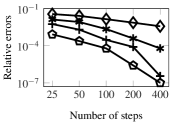
(a) Peer(1-4)

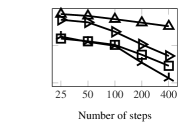
(b) RosPeer(1-4)

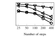
(c) mRosPeer(1-4)

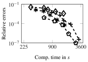
(d) Peer(1-4)

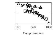
(e) RosPeer(1-4)

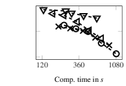
(f) mRosPeer(1-4)

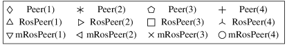
Figure 1: Steel profile: Accuracy and efficiency plots

Table 3: Steel profile: Computational timings and relative errors with respect to the reference solution for $\tau=0.1125\ s$, 400 steps.

Method	Time in $s$	Rel. Frobenius err.
BDF(1)	1 627.76	3.75e-03
BDF(2)	1 347.55	3.20e-04
BDF(3)	1 228.07	1.29e-04
BDF(4)	1 179.00	4.58e-05
Ros1	806.00	3.75e-03
Ros2	1 028.04	1.24e-03
Ros4	1 001.05	1.30e-06
Mid	1 239.78	1.33e-04
Trap	1 202.90	1.32e-04
Peer(1)	1 551.03	3.75e-03
Peer(2)	1 635.30	6.09e-05
Peer(3)	2 815.84	1.01e-07
Peer(4)	3 268.56	3.57e-07
RosPeer(1)	605.64	3.75e-03
RosPeer(2)	702.46	1.50e-05
RosPeer(3)	892.35	2.41e-06
RosPeer(4)	1 087.55	2.41e-07
mRosPeer(1)	610.31	3.75e-03
mRosPeer(2)	698.74	1.50e-05
mRosPeer(3)	883.33	2.41e-06
mRosPeer(4)	1 088.86	2.41e-07

As a first example, we consider a semi-discretized heat transfer problem for optimal cooling of steel profiles [10, 39]. This example is a mutli-input multi-output (MIMO) system with $m=7$ inputs and $q=6$ outputs. The solution to the DRE is computed on the simulation time interval $[0,\;4\,500]\ s$ with the step sizes $\tau\in\{180,90,45,25.5,12.75\}\ s$ and $\{25,50,100,200,400\}$ steps, respectively. Note that the actual time line is implicitly scaled by $1e2$ within the model such that a real time of $[0,45]\ s$ with corresponding step sizes is investigated. To ensure the computability of a reference solution in appropriate time, the smallest available discretization level with $n=371$ is chosen. The reference is computed by the small-scale dense version of the fourth-order Rosenbrock (Ros4) method. In particular, the Parareal based implementation with $450$ coarse and additionally $1000$ fine steps at each of those intervals, considered in [27], has been used.

Figures 1(1(a))-(1(c)) show the accuracy plots for the implicit peer methods, the RosPeer schemes and the modified RosPeer integrators, respectively. It can be observed that, for this example, the convergence orders are reached asymptotically. Further, note that the Peer(3) scheme outperforms its Peer(4) successor. This is due to the superconvergence of the Peer(3) method (see [51, Section 4, Method 3a]) and the fact that, for this example, the convergence order 4 of the Peer(4) scheme has just been reached for the last step size refinement. It can further be observed that the implicit peer and the Rosenbrock-type schemes of corresponding order achieve a comparable accuracy. This is not too surprising considering an autonomous problem. The efficiency plots are presented in Figures (1(d))-(1(f)). In Table 3, the LRSIF computation times and the relative errors with respect to the reference solution are given. Here, it becomes clear that the peer methods of order $s\geq 2$ show a significantly better performance compared to the other implicit time integrators of similar order with respect to the accuracy. Solely comparing the computational times, the Rosenbrock-type peer scheme of first-order shows best performance. Taking the efficiency into account, i.e., studying the required computational time versus the achieved error level, see also Figures 1(1(d))-(1(f)), the RosPeer schemes and its modified versions surpass the already existing LRSIF versions of the implicit integration schemes for DREs. Further, it is noteworthy that the fourth-order peer schemes do not reach better error levels that was already visible from Figures 1(1(a))-(1(c)). A more detailed investigation of all methods up to order $2$ and in particular the peer schemes can be found in [32].

4.2 Convection-diffusion - Small-Scale LTV

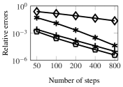
(a) Peer(1-4)

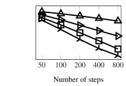
(b) RosPeer(1-4)

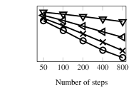
(c) mRosPeer(1-4)

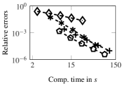
(d) Peer(1-4)

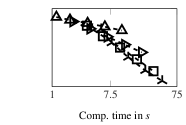
(e) RosPeer(1-4)

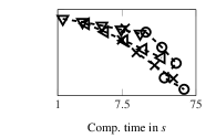
(f) mRosPeer(1-4)

Figure 2: Convection-diffusion LTV: Accuracy and efficiency plots

The second example is a convection-diffusion model problem originating from a centered finite differences discretization of the partial differential equation

$$\dot{v}=-\Delta v-f_{1}\frac{\partial v}{\partial\xi_{1}}-f_{2}\frac{\partial v}{\partial\xi_{2}}-f_{3}=0,$$ (28)

for $v=v(\xi_{1},\xi_{2})$ defined on the unit square $\Omega=(0,1)^{2}$ with homogeneous Dirichlet boundary conditions. Here, $f_{i},~{}i=1,2,3$, are functions depending on $\xi_{1},\xi_{2}$ and are often referred to as convection and reaction terms. The system matrices $A$ and $B,C$ are generated by the MATLAB routines fdm_2d_matrix and fdm_2d_vector, respectively, from LyaPack [41] with $n_{0}=9$ equidistant grid points for each spatial dimension, resulting in $n=n_{0}^{2}=81$ unknowns, and the convection and reaction terms are chosen as $f_{1}=20,~{}f_{2}=5,~{}f_{3}=0$. Further, the model represents a single-input single-output (SISO) system with $m=1$ input and $q=1$ output. The regions, where $B$ and $C$ act are restricted to the lower left corner $\xi_{1}\in(0,0.35),\xi_{2}\in(0,0.35)$ for the input and the upper area defined by $\xi_{1}\in(0,1),\xi_{2}\in(0.95,1)$ for the output, respectively. In order to obtain an LTV model, we introduce an artificial time-variability $\mu(t)=\frac{3}{4}\sin(8\pi t)+1\in[0.25,1.75]$ to the system matrix $A$. As a result, we obtain a time-varying system with constant matrices $E,B,C$ and a time dependent matrix $A(t)=\mu(t)A$. The model is simulated for the time interval $[0,0.5]\ s$ with the time step sizes $\tau\in\{\frac{1}{100},\frac{1}{200},\frac{1}{400},\frac{1}{800},\frac{1}{1600}\}\ s$, resulting in $\{50,100,200,400,800\}$ steps, respectively. As for the previous example, Figures 2(2(a))-(2(c)) show the error behavior with respect to the several time step sizes used. Here, the predicted convergence behavior is clearly visible except for the Peer(4) scheme. The efficiency plots are presented in Figures 2(2(d))-(2(f)). For this example, again the peer schemes show best performance with respect to the achieved accuracy. Additionally considering the computational effort of the integration schemes, the BDF methods show best performance up to order 3. See also Table 4. For large-scale model problems, the computational effort for solving the ARE inside the implicit schemes will become more expensive compared to the ALE solves within the linear implicit time integrators such that the latter will become more effective.

Table 4: Convection-diffusion LTV: Computational timings and relative errors with respect to the reference solution for $\tau=6.25e$-4 $s$, 800 steps.

Method	Time in $s$	Rel. Frobenius err.
BDF(1)	25.07	2.32e-02
BDF(2)	23.33	6.79e-04
BDF(3)	23.05	7.34e-05
BDF(4)	23.08	2.91e-05
Ros1	12.57	2.09e-02
Ros2	48.50	2.87e-03
Ros4	62.18	4.36e-04
Mid	29.46	1.91e-04
Trap	29.11	2.13e-04
Peer(1)	26.92	2.32e-02
Peer(2)	51.93	4.26e-05
Peer(3)	84.82	3.84e-06
Peer(4)	108.81	9.81e-06
RosPeer(1)	11.16	2.09e-02
RosPeer(2)	22.15	4.32e-04
RosPeer(3)	33.28	1.54e-05
RosPeer(4)	45.03	2.77e-06
mRosPeer(1)	13.09	2.09e-02
mRosPeer(2)	25.60	4.32e-04
mRosPeer(3)	37.00	1.54e-05
mRosPeer(4)	51.74	2.77e-06

4.3 Convection-Diffusion - Large-Scale LTI

Table 5: Convection-diffusion LTI: Computational timings for $\tau=6.25e$-4, 480 steps.

Method	Time in $s$
BDF(1)	1 260.43
BDF(2)	1 038.41
BDF(3)	870.76
BDF(4)	813.07
Ros1	1 107.56
Ros2	5 779.17
Ros4	10 571.82
Mid	793.03
Trap	796.44
Peer(1)	1 239.61
Peer(2)	1 322.49
Peer(3)	2 068.50
Peer(4)	2 652.84
RosPeer(1)	583.14
RosPeer(2)	561.36
RosPeer(3)	740.52
RosPeer(4)	913.28
mRosPeer(1)	584.07
mRosPeer(2)	543.07
mRosPeer(3)	647.03
mRosPeer(4)	887.04

The third example is again the convection-diffusion model (28) from Example 2. Here, the convection and reaction terms $f_{1}=50,~{}f_{2}=10,~{}f_{3}=0$ and no additional artificial time-variability are used. Further, $n_{0}=45$ grid nodes in each direction, yielding a system dimension of $n=2\,025$, are considered. The model is simulated for the time interval $[0,0.3]\ s$ with time step sizes $\tau\in\{\frac{1}{100},\frac{1}{200},\frac{1}{400},\frac{1}{800},\frac{1}{1600}\}\ s$, and $\{30,60,120,240,480\}$ steps, respectively. Due to the system size, no reference solution is computed. Similar to the previous examples, Table 4 shows the computational timings for the several integration schemes. Again, the Rosenbrock-type peer schemes up to order 3 come up with the lowest computational times. It can also be seen that for this autonomous SISO system, the reformulated Rosenbrock-type schemes (mRosPeer) outperform their counterparts given in the original formulation.

5 Conclusion

In this contribution, the classes of implicit and Rosenbrock-type peer methods have been applied to matrix-valued ODEs. Further, a reformulation of the latter has been proposed in order to avoid a number of Jacobian applications to the currently computed stage variables. An efficient low-rank formulation in terms of the low-rank symmetric indefinite factorization (LRSIF) has been presented. The performance of the peer methods was presented for three different examples. It has been shown that the Rosenbrock-type schemes and their reformulated version outperform their classical implicit one- and multi-step opponents with respect to the relation of accuracy and computational effort in most cases. Thus, the peer methods and in particular Rosenbrock-type schemes make an important contribution to the efficient low-rank based solution of differential Riccati equations and most probably differential matrix equations, in general.

References

- [1] H. Abou-Kandil, G. Freiling, V. Ionescu, and G. Jank, Matrix Riccati Equations in Control and Systems Theory, Birkhäuser, Basel, Switzerland, 2003.
- [2] A. C. Antoulas, D. C. Sorensen, and Y. Zhou, On the decay rate of Hankel singular values and related issues, Systems Control Lett., 46 (2002), pp. 323–342.
- [3] P. Benner, P. Kürschner, and J. Saak, Efficient handling of complex shift parameters in the low-rank Cholesky factor ADI method, Numer. Algorithms, 62 (2013), pp. 225–251, https://doi.org/10.1007/s11075-012-9569-7.
- [4] P. Benner, P. Kürschner, and J. Saak, An improved numerical method for balanced truncation for symmetric second order systems, Math. Comput. Model. Dyn. Sys., 19 (2013), pp. 593–615, https://doi.org/10.1080/13873954.2013.794363.
- [5] P. Benner, P. Kürschner, and J. Saak, Self-generating and efficient shift parameters in ADI methods for large Lyapunov and Sylvester equations, Electron. Trans. Numer. Anal., 43 (2014), pp. 142–162.
- [6] P. Benner, R.-C. Li, and N. Truhar, On the ADI method for Sylvester equations, J. Comput. Appl. Math., 233 (2009), pp. 1035–1045, https://doi.org/10.1016/j.cam.2009.08.108.
- [7] P. Benner and H. Mena, BDF methods for large-scale differential Riccati equations, in Proc. 16th Intl. Symp. Mathematical Theory of Network and Systems, MTNS, B. De Moor, B. Motmans, J. Willems, P. Van Dooren, and V. Blondel, eds., 2004.
- [8] P. Benner and H. Mena, Rosenbrock methods for solving Riccati differential equations, IEEE Trans. Autom. Control, 58 (2013), pp. 2950–2957.
- [9] P. Benner and H. Mena, Numerical solution of the infinite-dimensional LQR-problem and the associated differential Riccati equations, J. Numer. Math., 26 (2018), pp. 1–20, https://doi.org/10.1515/jnma-2016-1039. published online May 2016.
- [10] P. Benner and J. Saak, Linear-quadratic regulator design for optimal cooling of steel profiles, Tech. Report SFB393/05-05, Sonderforschungsbereich 393 Parallele Numerische Simulation für Physik und Kontinuumsmechanik, TU Chemnitz, D-09107 Chemnitz (Germany), 2005, http://nbn-resolving.de/urn:nbn:de:swb:ch1-200601597.
- [11] P. Benner and J. Saak, Numerical solution of large and sparse continuous time algebraic matrix Riccati and Lyapunov equations: a state of the art survey, GAMM Mitteilungen, 36 (2013), pp. 32–52, https://doi.org/10.1002/gamm.201310003.
- [12] J. C. Butcher, On the convergence of numerical solutions to ordinary differential equations, Math. Comp., 20 (1966), pp. 1–10.
- [13] J. C. Butcher, General linear methods: a survey, Appl. Numer. Math., 1 (1985), pp. 273–284, https://doi.org/10.1016/0168-9274(85)90007-8.
- [14] J. C. Butcher, General linear methods, Comput. Math. Appl., 31 (1996), pp. 105–112, https://doi.org/10.1016/0898-1221(95)00222-7.
- [15] E. J. Davison and M. C. Maki, The numerical solution of the matrix Riccati differential equation, IEEE Trans. Autom. Control, 18 (1973), pp. 71–73.
- [16] L. Dieci, Numerical integration of the differential Riccati equation and some related issues, SIAM J. Numer. Anal., 29 (1992), pp. 781–815.
- [17] V. Druskin, V. Simoncini, and M. Zaslavsky, Adaptive tangential interpolation in rational Krylov subspaces for MIMO dynamical systems, SIAM J. Matrix Anal. Appl., 35 (2014), pp. 476–498, https://doi.org/10.1137/120898784.
- [18] L. Grasedyck, Existence of a low rank or -matrix approximant to the solution of a Sylvester equation, Numer. Lin. Alg. Appl., 11 (2004), pp. 371–389.
- [19] E. Hairer and G. Wanner, Solving Ordinary Differential Equations II - Stiff and Differential-Algebraic Problems, Springer Series in Computational Mathematics, Springer-Verlag, second ed., 2002.
- [20] E. Hansen and T. Stillfjord, Convergence analysis for splitting of the abstract differential riccati equation, SIAM J. Numer. Anal., 52 (2014), pp. 3128–3139, https://doi.org/10.1137/130935501.
- [21] J. Harnard, P. Winternitz, and R. L. Anderson, Superposition principles for matrix Riccati equations, J. Math. Phys., 24 (1983), pp. 1062–1072.
- [22] A. Ichikawa and H. Katayama, Remarks on the time-varying Riccati equations, Systems Control Lett., 37 (1999), pp. 335–345.
- [23] O. L. R. Jacobs, Introduction to Control Theory, Oxford Science Publications, Oxford, UK, 2nd ed., 1993.
- [24] I. M. Jaimoukha and E. M. Kasenally, Krylov subspace methods for solving large Lyapunov equations, SIAM J. Numer. Anal., 31 (1994), pp. 227–251.
- [25] C. Kenney and R. B. Leipnik, Numerical integration of the differential matrix Riccati equation, IEEE Trans. Autom. Control, 30 (1985), pp. 962–970.
- [26] D. L. Kleinman, On an iterative technique for Riccati equation computations, IEEE Trans. Autom. Control, 13 (1968), pp. 114–115.
- [27] M. Köhler, N. Lang, and J. Saak, Solving differential matrix equations using parareal, Proc. Appl. Math. Mech., 16 (2016), pp. 847–848, https://doi.org/10.1002/pamm.201610412.
- [28] A. Koskela and H. Mena, A structure preserving Krylov subspace method for large scale differential Riccati equations, e-print arXiv:1705.07507, arXiv, May 2017, https://arxiv.org/abs/1705.07507. math.NA.
- [29] P. Kürschner, Efficient Low-Rank Solution of Large-Scale Matrix Equations, Dissertation, Otto-von-Guericke-Universität, Magdeburg, Germany, Apr. 2016, http://hdl.handle.net/11858/00-001M-0000-0029-CE18-2. Shaker Verlag, ISBN 978-3-8440-4385-3.
- [30] D. G. Lainiotis, Generalized Chandrasekhar algorithms: Time-varying models, IEEE Trans. Automat. Control, 21 (1976), pp. 728–732.
- [31] P. Lancaster and L. Rodman, The Algebraic Riccati Equation, Oxford University Press, Oxford, UK, 1995.
- [32] N. Lang, Numerical Methods for Large-Scale Linear Time-Varying Control Systems and related Differential Matrix Equations, Dissertation, Technische Universität Chemnitz, Germany, June 2017, https://www.logos-verlag.de/cgi-bin/buch/isbn/4700. Logos-Verlag, Berlin, ISBN 978-3-8325-4700-4.
- [33] N. Lang, H. Mena, and J. Saak, An factorization based ADI algorithm for solving large scale differential matrix equations, Proc. Appl. Math. Mech., 14 (2014), pp. 827–828, https://doi.org/10.1002/pamm.201410394.
- [34] N. Lang, H. Mena, and J. Saak, On the benefits of the factorization for large-scale differential matrix equation solvers, Linear Algebra Appl., 480 (2015), pp. 44–71, https://doi.org/10.1016/j.laa.2015.04.006.
- [35] A. J. Laub, Schur techniques for Riccati differential equations, in Feedback Control of Linear and Nonlinear Systems, D. Hinrichsen and A. Isidori, eds., Springer-Verlag, New York, 1982, pp. 165–174.
- [36] A. Locatelli, Optimal Control: An Introduction, Birkhäuser, Basel, Switzerland, 2001.
- [37] V. Mehrmann, The Autonomous Linear Quadratic Control Problem, Theory and Numerical Solution, no. 163 in Lecture Notes in Control and Information Sciences, Springer-Verlag, Heidelberg, July 1991.
- [38] H. Mena, Numerical Solution of Differential Riccati Equations Arising in Optimal Control Problems for Parabolic Partial Differential Equations, Ph.D. Thesis, Escuela Politecnica Nacional, 2007.
- [39] Oberwolfach Benchmark Collection, Steel Profile. hosted at MORwiki – Model Order Reduction Wiki, 2005, http://modelreduction.org/index.php/Steel_Profile.
- [40] T. Penzl, Eigenvalue decay bounds for solutions of Lyapunov equations: the symmetric case, Systems Control Lett., 40 (2000), pp. 139–144.
- [41] T. Penzl, Lyapack Users Guide, Tech. Report SFB393/00-33, Sonderforschungsbereich 393 Numerische Simulation auf massiv parallelen Rechnern, TU Chemnitz, 09107 Chemnitz, Germany, 2000. Available from http://www.tu-chemnitz.de/sfb393/sfb00pr.html.
- [42] I. R. Petersen, V. A. Ugrinovskii, and A. V. Savkin, Robust Control Design Using Methods, Springer-Verlag, London, UK, 2000.
- [43] H. Podhaisky, R. Weiner, and B. A. Schmitt, Rosenbrock-type ‘peer’ two-step methods, Appl. Numer. Math., 53 (2005), pp. 409–420, https://doi.org/10.1016/j.apnum.2004.08.021.
- [44] H. Podhaisky, R. Weiner, and B. A. Schmitt, Linearly-implicit two-step methods and their implementation in Nordsieck form, Appl. Numer. Math., 56 (2006), pp. 374–387, https://doi.org/10.1016/j.apnum.2005.04.024.
- [45] B. A. Schmitt and R. Weiner, Parallel two-step W-methods with peer variables, SIAM J. Numer. Anal., 42 (2004), pp. 265–282 (electronic), https://doi.org/10.1137/S0036142902411057.
- [46] B. A. Schmitt, R. Weiner, and K. Erdmann, Implicit parallel peer methods for stiff initial value problems, Appl. Numer. Math., 53 (2005), pp. 457–470, https://doi.org/10.1016/j.apnum.2004.08.019.
- [47] B. A. Schmitt, R. Weiner, and H. Podhaisky, Multi-implicit peer two-step -methods for parallel time integration, BIT, 45 (2005), pp. 197–217, https://doi.org/10.1007/s10543-005-2635-y.
- [48] L. F. Shampine, Implementation of Rosenbrock methods, ACM Transactions on Mathematical Software, 8 (1982), pp. 93–103.
- [49] S. Shokoohi, L. Silverman, and P. Van Dooren, Linear time-variable systems: balancing and model reduction, IEEE Trans. Automat. Control, 28 (1983), pp. 810–822.
- [50] V. Simoncini, Computational methods for linear matrix equations, SIAM Review, 58 (2016), pp. 377–441, https://doi.org/10.1137/130912839.
- [51] B. Soleimani and R. Weiner, A class of implicit peer methods for stiff systems, Journal of Computational and Applied Mathematics, 316 (2017), pp. 358 – 368, https://doi.org/https://doi.org/10.1016/j.cam.2016.06.014.
- [52] T. Stillfjord, Low-rank second-order splitting of large-scale differential Riccati equations, IEEE Trans. Autom. Control, 61 (2015), pp. 2791–2796, https://doi.org/10.1109/TAC.2015.2398889.
- [53] T. Stillfjord, Adaptive high-order splitting schemes for large-scale differential Riccati equations, Numerical Algorithms, (2017), https://doi.org/10.1007/s11075-017-0416-8.
- [54] K. Strehmel, R. Weiner, and H. Podhaisky, Numerik gewöhnlicher Differentialgleichungen, Vieweg+Teubner-Verlag, 2nd ed., 2012, https://doi.org/10.1007/978-3-8348-2263-5.
- [55] T. Stykel and V. Simoncini, Krylov subspace methods for projected Lyapunov equations, Appl. Numer. Math., 62 (2012), pp. 35–50, https://doi.org/10.1016/j.apnum.2011.09.007.
- [56] N. Truhar and K. Veselić, Bounds on the trace of a solution to the Lyapunov equation with a general stable matrix, Systems Control Lett., 56 (2007), pp. 493–503, https://doi.org/10.1016/j.sysconle.2007.02.003.
- [57] E. I. Verriest and T. Kailath, On generalized balanced realizations, IEEE Trans. Automat. Control, 28 (1983), pp. 833–844.