Phase correlations in chaotic dynamics
A Shannon entropy measure

Abstract

In the present work we investigate phase correlations by recourse to the Shannon entropy. Using theoretical arguments we show that the entropy provides an accurate measure of phase correlations in any dynamical system, in particular when dealing with a chaotic diffusion process. We apply this approach to different low dimensional maps in order to show that indeed the entropy is very sensitive to the presence of correlations among the successive values of angular variables, even when it is weak. Later on, we apply this approach to unveil strong correlations in the time evolution of the phases involved in the Arnold’s Hamiltonian that lead to anomalous diffusion, particularly when the perturbation parameters are comparatively large. The obtained results allow us to discuss the validity of several approximations and assumptions usually introduced to derive a local diffusion coefficient in multidimensional near–integrable Hamiltonian systems, in particular the so-called reduced stochasticity approximation.

1 Introduction

Chaotic diffusion in multidimensional near–integrable systems is a quite relevant dynamical process observed in different fields of astronomy, physics and chemistry. Particularly in dynamical astronomy, diffusion plays a major role in planetary and galactic dynamics, as recently reviewed and discussed in MCB16 , CGMB17 , MGCG18 and references therein. The characterization of this instability is still an open subject, phase correlations mainly due to stickiness, prevent in general the free diffusion that exhibits for instance an ergodic system, where the variance of any phase space variable, $\sigma^{2}$, increases linearly with time. This type of behavior is known in the literature as normal diffusion.

As shown in several works, it seems that in the limit of weak chaos, the diffusion that proceeds along the chaotic layer of a single resonance (or along different layers of the resonance web) over very large motion times might be approximated by a normal process (see for example LGF03 , FGL05 , GLF05 , FLG06 , LFG08 , EH13 and CEGM14 ), leading then to a slow drift of the unperturbed integrals of motion. On the other hand, in the strongly chaotic scenario and relatively short (or physical) motion times, diffusion could deviate significantly from the normal regime as it was presented in CGMB17 . This anomalous behavior of the diffusion imposes serious limitations on the derivation of a diffusion coefficient. Indeed, within this approach to the stability problem, the diffusion coefficient is introduced as the constant rate at which the variance evolves with time.

Let us mention that anomalous diffusion has been observed also in many low dimensional dynamical systems. In for instance Z94 ,ZA95 , ZEN97 , ZN97 , ZE00 and Z02 as well as in KBZS90 , KZS93 , KK04 , SGM17 , V08 , MSV14 , a different approach to diffusion is considered through a transport process formulation, where a generalization of the normal regime is introduced, i.e. the variance scales as $\sigma^{2}=Dt^{b}$ where the value of the exponent $b$ determines the regime of anomalous transport, namely super–diffusion if $b>1$ or sub–diffusion when $b<1$, and the diffusion coefficient $D$ is thus defined.

In GC18 we present an alternative way to measure both, the extent and the time rate of chaotic diffusion by means of the Shannon entropy (see SW49 ). A relevant aspect of this approach is that the time evolution of the entropy is independent of the transport process that takes place in phase space and therefore a measure of the diffusion rate could be derived independently of the power law the variance satisfies.

In any case, as we have already mentioned, phase correlations are responsible for anomalous diffusion. The analysis of phase correlations is a quite difficult problem and thus restrictive assumptions are adopted in order to obtain analytical estimates for local diffusion coefficients (see for instance Ch79 , C02 , CEGM14 ). Therefore, herein we face with the problem of phase correlations in order to get some insight on the time evolution of chaotic diffusion.

While the time–correlation function (see for instance D87 , R98 ) seems to be an appropriate tool to quantify phase correlations, its computation is not an easy task (as shown for example in BH70 ) and its numerical implementation is in fact quite expensive. Thus, in the present effort, also by recourse to the Shannon entropy, we provide a very efficient and simple way to clearly detect phase correlations.

In Section 2 we outline the underneath theory of the Shannon entropy in a similar fashion as that given in GC18 , while in Section 3 profuse numerical experiments are presented in several well known maps to finally investigate phase correlations in the Arnold’s Hamiltonian A64 , the very same system studied in CGMB17 and GC18 . In this direction, we discuss the limitations of the assumptions behind the analytical derivation of expressions for a local diffusion coefficient in Chirikov’s formulation of Arnold Diffusion Ch79 .

2 The Shannon entropy

As we have already discussed, it is not a simple task to provide a measure of correlations among successive values of a dynamical variable, in particular at large times. Thus, in the present section we propose the Shannon Entropy as an efficient tool to measure correlations.

Theoretical background on the Shannon entropy can be found in SW49 however, different approaches to the entropy in dynamical systems are presented in, for instance, K67 , AA89 and W78 . Applications to time series analysis can be found in CHMNV99 and C99 . A recent approach concerning the use of the Shannon entropy to measure chaotic diffusion and its time rate is addressed in GC18 .

Following for instance AA89 and L14 , consider the function $Z$ defined in $[0,1]$ as:

$$Z(x)=\begin{cases}-x\,\mathrm{ln}x,\qquad&x\in(0,1]\\ \\ 0\qquad&x=0.\end{cases}$$ (1)

It is evident that $Z(x)\geq 0$ and $Z^{\prime\prime}<0$. Consider now an open domain $B\in\mathbb{R}^{n}$ and let

$$\alpha\,=\,\{a_{i};\,i=1,\cdots,q\}$$ (2)

be a partition of $B$, let us say a collection of $q$ $n$-dimensional cells that completely cover $B$. The elements $a_{i}$ are assumed to be both measurable and disjoint. We consider $n=1$ and $B=\mathbb{S}^{1}$ or the unit interval $(0,1)$ with opposite sides identified.

Let $x_{i}=x(t_{i})$ be the phase variable of a given map $M$ (or Hamiltonian flow) such that $(y_{n},x_{n})\,\to\,(y_{n+1},x_{n+1})$, with $y\in G\subset\mathbb{R}$ some action variable .

For any finite trajectory $\gamma=\{(y_{i},x_{i})\in G\times B,i=1,\dots,N\}$ of $M$, let us define $\gamma_{x}=\{x_{i}\in B,i=1,\dots,N\}\subset\gamma$, then a probability density on $B$ can be defined as

$$\rho({u},\gamma_{x}),=\,\frac{1}{N}\sum_{i=1}^{N}\delta({u}-{{x}}_{i}),$$ (3)

where $\delta$ denotes the delta function. It is clear that

$$\int_{B}\;\rho({u},\gamma_{x})\,d{u}\,=\,1,$$ (4)

and the measure $\mu(a_{i})$ results

$$\mu(a_{i}(\gamma_{x}))\,=\,\int_{a_{i}}\;\rho({u},\gamma_{x})\,d{u}.$$ (5)

Then, for the partition $\alpha$ the entropy for $\gamma_{x}$ is defined as

$$S(\gamma_{x},\alpha)\,=\,\sum_{i=1}^{q}\,Z\left(\,\mu(a_{i}(\gamma_{x}))\,\right)\,=\,-\sum_{i=1}^{q}\,\mu(a_{i}(\gamma_{x}))\,\ln(\mu(a_{i}(\gamma_{x}))).$$ (6)

Notice that for a given partition and trajectory, the entropy is bounded. Indeed, for the partition (2) it is $0\leq S(\gamma_{x},\alpha)\leq\ln q$, for any $\gamma_{x}$. The minimum corresponds to the situation in which the $x_{i}$ are restricted to a single element of $\alpha$, say the $j$–th element, which would correspond to the extreme case of full correlation of the phase values at all times, such as for example at a first order resonance or one-period fixed point of $M$ ($x_{n+1}=x_{n},\forall n$). In such a case it is $\mu(a_{j})=1,\mu(a_{i})=0,\forall i\neq j$, leading to $S=0$. On the other hand, the maximum value, $S=\ln q$, would be obtained when the $q$ elements of the partition had an equal measure, that is $\mu(a_{j})=1/q$, which corresponds to the situation in which the $x$ values are dense and uniformly distributed in $B$. Therefore, in the case of a non-integrable system, the entropy seems to be a natural measure of correlations.

Let $n_{k}$ be the number of phase values in the cell $a_{k}$, then $\mu(a_{k})=n_{k}/N$. From the normalization condition, $\sum_{k=1}^{q}\mu(a_{k})=1,$ it follows that $\sum_{k=1}^{q}n_{k}=N.$ Therefore, the entropy given in (6) reduces to

$$S(\gamma_{x},\alpha)=\ln N-\frac{1}{N}\sum_{k=1}^{q}n_{k}\ln n_{k}.$$ (7)

Take for instance $\gamma_{x}^{r}=\{x_{i}=\theta^{r}_{i}\in B,i=1,\dots,N\}$ where the $\theta^{r}_{i}$ are random numbers and $N\gg 1$, then the $n_{k}$ obey a Poisson distribution:

$$P_{\lambda}(n)=\frac{\lambda^{n}}{n!}\mathrm{e}^{-\lambda},\qquad\lambda=\frac{N}{q},$$

where $\lambda$ is the mean value of the distribution as well as its variance. Let us assume $\lambda\gg 1$ and take $n_{k}=\lambda+\xi_{k}$ with $|\xi_{k}|\ll\lambda$ ($n_{k}\in\mathbb{R}$), so

$$\sum_{k=1}^{q}\xi_{k}=0,$$ (8)

which clearly follows from the normalization condition. Then it is straightforward to show that, up to second order in $\xi_{k}/\lambda$, it is

$$\sum_{k=1}^{q}n_{k}\ln n_{k}=N\ln N-N\ln q+\frac{1}{2\lambda}\sum_{k=1}^{q}\xi_{k}^{2},$$ (9)

and (7) reads

$$S(\gamma_{x}^{r},\alpha)=\ln q-\frac{q}{2N^{2}}\sum_{k=1}^{q}\xi_{k}^{2}.$$ (10)

Now on introducing the information $\mathcal{I}$ as

$$\mathcal{I}(\gamma_{x},\alpha)\equiv 1-\frac{1}{\ln q}S(\gamma_{x},\alpha),$$ (11)

and estimating $\xi_{k}^{2}=\lambda$ we get, in this particular limit of absence of correlations, that

$$\mathcal{I}(\gamma_{x}^{r},\alpha)\approx\frac{q}{2N\ln q}>0,$$ (12)

which results independent of $\gamma_{x}^{r}$. Since $N$ denotes the number of iterates of the map, we observe that, for completely random motion, $\mathcal{I}$ would decrease with time as $t^{-1}$.

On the other hand, from (6) the time derivative of the entropy results

$$\frac{dS}{dt}(\gamma_{x},\alpha)=-\sum_{k=1}^{q}\dot{\mu}(a_{k})(1+\ln\mu(a_{k})),$$ (13)

and, for random motion, its theoretical estimate is

$$\frac{dS}{dt}(\gamma_{x}^{r},\alpha)\approx\frac{q}{2N^{2}}\dot{N}>0,$$ (14)

which is seen to decrease as $t^{-2}$.

The above results clearly state that, for a random system, the information decreases as time increases, or alternatively, the entropy would reach asymptotically its maximum value; the system approaches the full mixing as $t^{-1}$.

Now let us consider $\gamma_{x}^{s}=\{x_{i}=\theta^{s}_{i}\in B,i=1,\dots,N\}$ with $N\gg 1$ and where $\theta^{s}_{i}$ are correlated phases, for instance $\theta^{s}=\omega t$ with $\omega\in\mathbb{R}\setminus\mathbb{Q}$, which represents the motion on a torus. Being $\omega$ irrational, the motion is ergodic on $\mathbb{S}^{1}$, thus the distribution function of $n\in\mathbb{R}$ approaches $f(n_{k})\approx\delta(n_{k}-\lambda)$, with $\lambda=N/q$. Therefore, if we consider again $n_{k}=\lambda+\xi_{k}$ with $|\xi_{k}|\ll\lambda$, up to second order in $\xi_{k}/\lambda$, (10) holds. The fluctuations should satisfy $|\xi_{k}|<1$, since every $n_{k}$ would be the closest integer number to $\lambda$ which, in general, is a real quantity. Therefrom, setting $|\xi_{k}|\approx 1/2$, the information (12) for a single quasiperiodic trajectory on the torus reduces to

$$\mathcal{I}(\gamma_{x}^{s},\alpha)\approx\frac{q^{2}}{8N^{2}\ln q},$$ (15)

and, in this particular case, the information would decrease as $t^{-2}$. Notice that if we consider instead an ensemble of $n_{p}$ nearby trajectories, the estimate $|\xi_{k}|\approx n_{p}/2$ has to be adopted (see below) and since $N=n_{p}\times t$, (15) becomes

$$\mathcal{I}(\gamma_{x}^{s},\alpha)\approx\frac{q^{2}}{8\ln q}\frac{1}{t^{2}}.$$ (16)

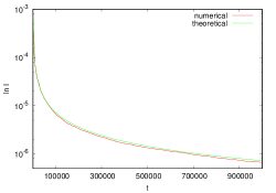
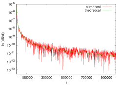
Figure 1: Left panel: evolution of $\mathcal{I}$ for $n_{p}=100$ initial values of $x_{i}\in(0,1)$ evolving randomly (in red) and the expected theoretical trend given by (12) with $N=n_{p}\times t$ (in green). Right panel: the time derivative of the entropy computed numerically (in red) and the theoretical evolution given by (14) (in green), see text for details.

In order to check the analytical estimates given in (12) and (14), we pick up $n_{p}=100$ initial values of the phases $x_{i}\in(0,1)$ and evolve each initial condition in a random way taking $x\leavevmode\nobreak\ \mathrm{mod}\leavevmode\nobreak\ 1$ to finally compute the information given by (11) and the derivative of the entropy every $\Delta t=10^{3}$. The information $\mathcal{I}$ for the ensemble corresponding to a partition $\alpha$ defined by $q=10^{3}$ cells on the unit interval, is computed for $N=n_{p}\times t$, where $t=10^{3},\dots,10^{6}$. The time derivative of the entropy can be evaluated, either from equation (13) or by the numerical derivative corresponding to the time evolution of (6), also every $\Delta t=10^{3}$. In fact, both results completely agree, though the latter procedure results somewhat less noisy than the former, so from now on we will restrict ourselves to show solely the numerical derivative of the entropy. Fig. 1 displays the results concerning the numerical simulation and the theoretical estimates for both the information and the time derivative of $S$, revealing the consistency of the proposed analytical approach.

Now, let us consider a similar example as the one above but for the 1D-map $x_{n+1}=x_{n}+\omega$ with $x\leavevmode\nobreak\ \mathrm{mod}\leavevmode\nobreak\ 1$ and $\omega\in\mathbb{R}$. We have carried out several experiments, taking different values of $n_{p}$ ranging from $1$ to $2000$, ensembles of size $10^{-5}$ to $10^{-9}$ and varying both $\Delta t$ and $q$. The outcome values of $\mathcal{I}$ given by (11) show to be only sensitive to the partition as (16) foresees, and to the $\omega$ value which could be either rational or irrational. For the particular case $\omega=l\in\mathbb{Z}$ we obtain $\mathcal{I}\approx 1\leavevmode\nobreak\ (S\approx 0)$ despite of the size of the partition $q>1$.

In Fig. 2 we present the representative behavior of $\mathcal{I}$ corresponding to ergodic motion on a torus for different $n_{p}$ values in ensembles with $|\omega-\sqrt{3}|\leq 10^{-8}$, $x_{0}=0$ and $N=n_{p}\times t$, $t=5\times 10^{3},\dots,5\times 10^{6}$, for a partition of the unit interval of $q=2\times 10^{3}$ and $\Delta t=5\times 10^{3}$. We also include in the figure the theoretical estimates given by (16). Again, we notice a good agreement between the numerical and theoretical estimates for the information in the case of ergodic motion.

The above examples, though rather simple, allow us to assert that in a non-linear system the information, that measures the phase correlations, should decrease at most as $t^{-1}$, the limit taking place when the system becomes completely mixed. Strong phase correlations would provide larger values of the information and $\mathcal{I}$ should scale with time as $\mathcal{I}\sim t^{\beta},\beta>-1$. On the other hand, if $\beta\to-2$, the phase evolves as in an integrable system, the successive values of $x$ though fully correlated are ergodic on the torus and so that the approximation $\langle\sin^{2}x\rangle=\langle\cos^{2}x\rangle\approx t/2$ holds, though this result does not imply that the phase values are completely uncorrelated.

[scale=0.6]regular3_x.eps

Figure 2: Evolution of $\mathcal{I}$ for three different $n_{p}$ values, $|\omega-\sqrt{3}|\leq 10^{-8}$ and $q=2000$ given by the map $x_{n+1}=x_{n}+\omega$ with $x_{0}=0$, and the expected theoretical trend for ergodicity given by (16) which is independent of $n_{p}$.

3 Numerical experiments

In this section we describe the numerical experiments regarding three different maps and provide evidence of how the information succeeds in yielding a measure of phase correlation in each case.

3.1 The standard map

This well known discrete area preserving dynamical system, introduced by Chirikov in Ch69 , Ch79 and largely studied in the last four decades (see for instance MSV14 and references therein), $(I,\theta)\to(I^{\prime},\theta^{\prime}),\,$ is defined by

$$I^{\prime}=I+K\sin\theta,\qquad\theta^{\prime}=\theta+I^{\prime},$$ (17)

with $I\in\mathbb{R},\,\theta\,\,\mathrm{mod}\,\,2\pi$, and $K$ a free parameter. We numerically investigate this system which describes the dynamics of a pendulum perturbed by an infinite set of periodic kicks of similar amplitude and frequency $\Omega=1$. In fact we deal with the reduced standard map defined in $\mathbb{S}^{1}\times\mathbb{S}^{1}$ as a consequence of introducing the new variables $(p,x)$ that comply $I=2\pi p,\,\theta=2\pi x$, both $p\,$ and $x\,\,$ being $\mathrm{mod}\,\,1$, so that

$$p^{\prime}=p+k\sin 2\pi x,\qquad x^{\prime}=x+p^{\prime},\qquad k=\frac{K}{2\pi}.$$ (18)

It is well known that for $K<1\,$ $\,(k<1/2\pi)$ the motion is mostly stable, except near the thin chaotic layers or homoclinic tangles around the integer resonance $p=0$ of size $\sqrt{k}$, and the main fractional resonances $p=1/2$ and $p=1/3,2/3$, whose half-widths are $k$ and $k^{3/2}$ respectively. For $K=K_{c}\approx 1$ the overlap of resonances becomes relevant and this critical value separates stable from unstable motion in a broad sense. For $K>4$ the centers of the integer resonances become unstable and therefrom the motion is usually assumed to be almost completely uncorrelated.

We have performed several numerical experiments with values of $K$ in the interval $0\leq K\leq 100$ though herein we only show a few examples corresponding to $K=0.1,1,5,10$, for an ensemble of $n_{p}=100$ random initial conditions with $p,x\approx 10^{-5}$. We have iterated the map (18) up to $N=10^{6}$, introducing a partition defined by $q=10^{3}$, and we have computed the information (11) and the derivative of the entropy (13) adopting a time interval of $\Delta=10^{3}$. The results are displayed in Fig. 3, where we have also included the theoretical estimates (12) and (14) for $\mathcal{I}$ and $dS/dt$ respectively, which correspond to the case of random motion, for a partition defined by $q$ and $N=n_{p}\times t$. The left panel shows the evolution of the information corresponding to different $K$ values. Notice that the phase values appear to be correlated for the lower values of $K$; in fact, even for $K$ values as large as $1$ or $5$ the successive values of the phases seem to be correlated for large times. A similar result is obtained for $K=9$ (not shown in the figure), but for $K\geq 10$ the dynamics in $x$ looks like random, the information decaying as $t^{-1}$. The right panel of Fig. 3 corresponds to the time derivative of the entropy. Besides the expected noisy behavior, it turns out evident that $dS/dt$ decreases as $t^{-2}$ only for the experiment corresponding to $K=10$. These results suggest that the usual assumption for the standard map,

$$\langle(I(t)-I(0))^{2}\rangle=K\sum_{l=1}^{t}\langle\sin^{2}\theta(l)\rangle\approx\frac{K}{2}t,$$

is a plausible approximation only for $K\gtrsim 10$, which is in agreement with the results given in MSV14 .

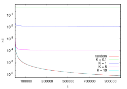
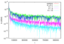
Figure 3: (Left panel) Evolution of $\mathcal{I}$ for $n_{p}=100$ initial values of $x_{i}\in(0,1)$ of the reduced standard map (18) for different values of the parameter $K$ and the analytical expected behavior for random motion given by (12) displayed in red for $N=n_{p}\times t$. (Right panel) Similar to the plot at the left but for the time derivative of the entropy computed numerically and the theoretical expected evolution given by (14).

3.2 The whisker mapping

Let us consider another canonical map, the whisker or separatrix mapping $(w,\tau)\to(w^{\prime},\tau^{\prime}),w\in\mathbb{R},\,\tau\,\,\mathrm{mod}\,\,2\pi$, also introduced by Chirikov in Ch69 ,Ch79 as

$$w^{\prime}=w+W\sin\tau,\qquad\tau^{\prime}=\tau+\lambda\ln\left(\frac{32}{|w^{\prime}|}\right),$$ (19)

where $W,\lambda$ are free parameters. This map represents the motion close to the separatrix of a non-linear resonance or pendulum subjected to a symmetric periodic perturbation; thus $|W|\sim A_{2}(\lambda)\ll 1$ for $\lambda\gg 1,$ where $A_{2}(\lambda)$ is the Melnikov-Arnold integral for $m=2$. This simple system models the chaotic layer around resonances. After rescaling the a-dimensional energy $w$ by $\lambda W$ and defining $y=w/(\lambda W)$, the mapping (19) reduces to

$$y^{\prime}=y+\frac{1}{\lambda}\sin\tau,\qquad\tau^{\prime}=\tau-\lambda\ln|y^{\prime}|+G,$$ (20)

where $G=\lambda\ln(32/\lambda|W|)$ is a constant. It is well known that, after the above rescaling, the chaotic layer has a finite width, $|y|\lesssim 1$, whose central part, $|y|\lesssim 1/4$, is highly chaotic, with no stability domains, while its external part reveals a divided phase space with large stability islands. Therefore, the strong correlation between the successive values of the phase $\tau$ for $|y|\sim 1$ should be responsible for the finite width of the layer. Roughly, near the edges of the layer it is $|y|\approx 1$ and thus from the second relation in (20) it is clear that the structure of the external part of the layer is dominated by $G$. Anyway, the study of its resonances, $y_{r_{k}}=(32/\lambda W)\exp(-2k\pi/\lambda)=\exp((G-2k\pi)/\lambda)),$ $k\in\mathbb{Z}$, by means of local standard maps clearly shows that the motion for $|y|\approx 1$ or larger should be mostly regular. Therefore it turns out fairly interesting to study phase correlations in this particular map by means of the Shannon entropy.

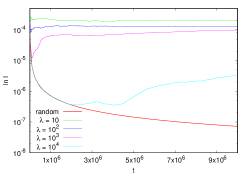
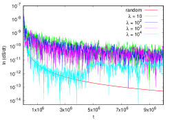
Figure 4: (Left panel) Evolution of $\mathcal{I}$ for $n_{p}=100$ initial values of $x_{i}\in(0,1)$ of the whisker mapping (20) for $W=10^{-6}$ and four different values of the parameter $\lambda$. The analytical expected behavior for random motion given by (12) is also included and displayed in red for $N=n_{p}\times t$. (Right panel) Similar to the plot at the left but for the time derivative of the entropy computed numerically and the theoretical expected evolution given by (14).

Then, we have thoroughly investigated the map (20) by numerical means taking different values of the parameters $W$ and $\lambda$. Herein we include the results concerning a single value of $W$, namely $W=10^{-6}$, since the map is almost independent of this scaling parameter, and four different values of $\lambda=10,10^{2},10^{3},10^{4}$. As before, we have considered an ensemble of $n_{p}=100$ random initial conditions with $(y,\tau)\approx 10^{-5}$. We have iterated the map up to $N=10^{7}$, after introducing the normalized phase $x=\tau/2\pi\,\mathrm{mod\leavevmode\nobreak\ 1}$, having taken a similar partition of the unit interval, $q=10^{3}$, and computed the information (11) and the derivative of the entropy (13) with a sample time interval $\Delta=10^{4}$. The results are displayed in Fig. 4, where again we have included the theoretical estimates (12) and (14) corresponding to random motion for $\mathcal{I}$ and $dS/dt$ respectively. In any case, the information reveals that at short times, while the trajectories are confined to the central part of the layer, the values of the phase $\tau$ seem to be uncorrelated, but for large times instead, when the system has already reached the border of the layer, the correlations are quite evident, the information $\mathcal{I}$ increasing significantly. Notice that the time required to become a correlated system is seen to increase with $\lambda$, as expected. The derivative of the entropy reveals the very same dynamical behavior.

3.3 A generalized whisker mapping

We devote this section to the numerical study of the map that describes, accordingly to Chirikov, the diffusion across and along the chaotic layer of the resonance $\omega_{1}=0$ for the Arnold Hamiltonian (see A64 , Ch79 ), which can be recast as

$$H(I_{1},I_{2},\theta_{1},\theta_{2},t;\varepsilon,\mu)=\frac{1}{2}(I_{1}^{2}+I_{2}^{2})+{\varepsilon}(\cos\theta_{1}-1)[1+{\mu}(\sin\theta_{2}+\cos t)],$$ (21)

with $I_{1},I_{2}\in\mathbb{R},\;\;\theta_{1},\theta_{2},t\in\mathbb{S}^{1}$, and $\mu\varepsilon\ll\varepsilon\ll 1$. Let us note that (21) can be re-arranged as

$$H(I_{1},I_{2},\theta_{1},\theta_{2},t;\varepsilon,\mu)=H_{1}(I_{1},\theta_{1};\varepsilon)+H_{2}(I_{2})+\mu V(\theta_{1},\theta_{2},t;\varepsilon),$$

where

$$H_{1}=\frac{1}{2}I_{1}^{2}+{\varepsilon}(\cos\theta_{1}-1),\qquad H_{2}=\frac{1}{2}I_{2}^{2},\qquad V={\varepsilon}(\cos\theta_{1}-1)(\sin\theta_{2}+\cos t),$$

and that the instantaneous change of $H$ and $H_{2}$ are given by

$$\dot{H}=\mu\frac{\partial V}{\partial t},\qquad\dot{H_{2}}=I_{2}\dot{I_{2}}=-\mu\omega_{2}\frac{\partial V}{\partial\theta_{2}},$$

where $\omega_{2}=I_{2}\neq 0$ is assumed to be constant and irrational, then

$$\dot{H} = \frac{\mu\varepsilon}{2}\left(2\sin t+\sin(\theta_{1}-t)-\sin(\theta_{1}+t)\right),$$

$$\dot{H}_{2} = \frac{\mu\varepsilon}{2}\left(2\omega_{2}\cos\theta_{2}-\cos(\theta_{2}-\theta_{1})-\cos(\theta_{2}+\theta_{1})\right).$$

Thus, taking $\theta_{2}(t)\approx\omega_{2}t+\theta_{2}^{0}$, $\theta_{1}(t)=4\arctan\left(\exp\left(\sqrt{\varepsilon}(t-t_{0})\right)\right)$, i.e. the motion on the separatrix, defined in such a way that $\theta_{1}=\pi$ for $t=t_{0}$, and neglecting the free oscillatory terms $\sin t$ and $\cos\theta_{2}$ , the variations of $H$ and $H_{2}$ over a half–period of oscillation of $\theta_{1}$ result (see Ch79 for more details)

$$\Delta H=\frac{\sqrt{\epsilon}\mu}{2}A_{2}\left(\frac{1}{\sqrt{\epsilon}}\right)\sin t^{0},\qquad\Delta H_{2}=\frac{\sqrt{\epsilon}\mu\omega_{2}}{2}A_{2}\left(\frac{\omega_{2}}{\sqrt{\epsilon}}\right)\cos\theta_{2}^{0},$$

where $t^{0}$ is the value of the phase $t$ when the pendulum crosses the surface $\theta_{1}=\pi$ where the stable equilibrium point lies, and $\theta_{2}^{0}=\theta_{2}(t^{0})$.

In Chirikov’s formulation, significant changes in $H$ are only possible due to large variations in $H_{2}$, since $H_{1}$ is bounded to the exponentially small (wrt $\mu$) width of the chaotic layer. Moreover, defining $D_{H}=\langle(H(t)-H(0))^{2}\rangle/t$ and $D_{2}=\langle(H_{2}(t)-H_{2}(0))^{2}\rangle/t$, for large times it should be $D_{H}=D_{2}$ and thus

$$\langle\sin^{2}t^{0}\rangle=v^{2}\langle\cos^{2}\theta_{2}^{0}\rangle,$$ (23)

with

$$v=\frac{\omega_{2}A_{2}\left(\frac{\omega_{2}}{\sqrt{\varepsilon}}\right)}{A_{2}\left(\frac{1}{\sqrt{\varepsilon}}\right)}=\omega_{2}^{2}\,\,\frac{\sinh\left(\pi/\sqrt{\varepsilon}\right)}{\sinh\left(\omega_{2}\pi/\sqrt{\varepsilon}\right)}\,\,e^{\frac{(\omega_{2}-1)\pi}{2\sqrt{\varepsilon}}}\,\approx\omega_{2}^{2}\,e^{\frac{(1-\omega_{2})\pi}{2\sqrt{\varepsilon}}},$$ (24)

where the approximation holds for $\varepsilon\ll 1$. The latter expression for the relative amplitude $v$ is significant only in the interval $|\omega_{2}-\omega_{2M}|<\sqrt{2\epsilon/\pi}$ where $\omega_{2M}=4\sqrt{\varepsilon}/\pi$ corresponds to its maximum value, being the latter $v_{M}\approx(4/\pi e)^{2}\varepsilon\exp\left(\pi/(2\sqrt{\varepsilon})\right)$; and goes to zero in both limits as $v\sim\omega_{2}^{2},\,\omega_{2}\to 0$ and as $v\sim\exp\left(-\omega_{2}/\sqrt{\varepsilon}\right),\,\omega_{2}\to\infty$. Then, for $\omega_{2}>1$ it is $v\ll 1$. On the other hand, for $\omega_{2}$ in the narrow range $\omega_{2}\approx\sqrt{\epsilon}\left(4/\pi\pm\sqrt{2/\pi}\right)$, it is $v\gg 1$. Therefore from (23) for $\omega_{2}$ away from $0$ and $1$, it turns out that both phases could not be simultaneously random.

The associated map represents the finite variation of the energy in $H_{1}$ (pendulum model for the resonance $\omega_{1}=0$) when the system is close to the separatrix of the resonance $\omega_{1}=0$ and it can be computed as the difference $\Delta H_{1}=\Delta H-\Delta H_{2}$ after a half period of oscillation or a period of rotation of the pendulum and it has the form $(y,\tau)\to(y^{\prime},\tau^{\prime})$,  $y\in\mathbb{R},\,\tau\,\mathrm{mod\leavevmode\nobreak\ 2\pi}$, where $y$ measures the energy changes in $H_{1}$ relative to the separatrix energy ($H_{1}=0$), $\tau$ represents the successive values of $t^{0}$ and it reads

$$y^{\prime}=y+\sin\tau-v\cos(\omega_{2}(\tau+\beta)),\qquad\tau^{\prime}=\tau-\frac{1}{\sqrt{\varepsilon}}\ln|y^{\prime}|+\eta,$$ (25)

where $\eta$ is a constant similar to $G$ introduced in the whisker mapping, that depends on both $\mu$ and $\varepsilon$ but not on $\omega_{2}$, $\omega_{2}\beta$ being the initial value of $\theta_{2}^{0}$.

Chirikov proposed that the map (25) not only describes the thin chaotic layer around the main or guiding resonance $\omega_{1}=0$ but the diffusion along the latter as well. For $\varepsilon\ll 1$ and $\omega_{2}>1\,(0<\omega_{2}\sim 4\sqrt{\varepsilon}/\pi)$ since $v\ll 1\,(v\gg 1)$, in the right hand side of the first equation of (25) a clearly dominant term is present. Thus at this order, the map reduces to the whisker mapping, being the largest term (layer resonances in Chirikov’s terminology) responsible for the properties of the chaotic layer, such as its width and resonances’ structure. Therefore, for large times, the successive values of the phase involved in such a dominant term would be strongly correlated ($\tau$ for $\omega_{2}\gg 1$ and $\theta_{2}$ for $\omega_{2}\sim 4\sqrt{\varepsilon}/\pi$). Note that for $v\ll 1\,(\omega_{2}\gg 1)$ the map becomes independent of $\omega_{2}$ and thus, while $\tau$ values should present correlations, phase values $\theta_{2}^{0}=\omega_{2}\tau$ could evolve, in principle, nearly in a random or ergodic fashion when $\omega_{2}$ is irrational and large.

Since when the system is close to the separatrix of the resonance $\omega_{1}=0$, the variation in $H_{1}$ is given by the largest term in the map ($y$), the successive values of the smaller term in the first of (25) are assumed to be nearly random, and this perturbation term (or driving resonances accordingly Chirikov) is responsible for a nearly normal diffusion process along the resonance, i.e. large variations in $I_{2}$ such that $\langle(H(t)-H(0))^{2}\rangle\propto t$ as in the standard map. In other words, for $\omega_{2}\sim 4\sqrt{\varepsilon}/\pi<1$ it is assumed that $\langle\sin^{2}\tau\rangle=R/2$, while for $\omega_{2}>1,\langle\cos^{2}\theta_{2}^{0}\rangle=R/2$, where $R<1$ is the so–called reduction factor that takes into account some correlations among the successive phase values when the system is moving within the external part of the chaotic layer (see Ch79 , C02 , CEGM14 ).

Let us remark that the derivation of the map (25) rests, among other simplifications, on the following assumptions: (i) $\varepsilon\ll 1$ such that no overlapping with other first order resonance takes place (as for instance among the resonances $\omega_{1}=\pm 1$ and $\omega_{1}=0$); (ii) $\varepsilon\mu\ll 1$ such that we could consider $\omega_{2}$ nearly constant and (iii) $|I_{2}|\gg 2\sqrt{\varepsilon\mu}$, the width of the resonance $\omega_{2}=0$, such that $\cos\theta_{2}$ can be regarded as a purely oscillatory term.

Therefore, the expected behavior of both phases depending on $\omega_{2}$ encourages the investigation of correlations in this map by means of the Shannon entropy.

We present the results of only one of the large set of experiments performed for $\varepsilon=0.05$ and $\mu=10^{-3}\varepsilon$ and eight different values of $\omega_{2}^{0}=\kappa\sqrt{3},\kappa\in K$ where

$$K=\{\kappa:\kappa=0.06,\,0.16,\,0.25,\,0.62,\,1.75,\,2.25,\,11.0,\,19.0\},$$

such that $0.10\lesssim\omega_{2}^{0}\lesssim 33$ and for $\kappa=0.62,\omega_{2}\approx 1$. For these values of $\varepsilon$ and $\kappa\in K$, the relative amplitude $v$ (24) ranges from $2\times 10^{-95}$ for the largest $\kappa$ value up to $12$ for $\kappa=0.16$, which it is in agreement with the analytical estimates given above. The resonances’ width is about $0.447$ for the resonance $\omega_{1}=0$ while it equals $0.003$ for the remainder ones, so that no overlap would be expected between the main resonance and $\omega_{1}=\pm 1$. For the smallest value of $\kappa\in K$, $\omega_{2}^{0}\approx 0.104$ and it would be plausible to assume that it is far from the resonance $\omega_{2}=0$ since its width is quite small. Anyway, we numerically integrated the Hamiltonian (21) for the same set of parameters and $n_{p}=100$ random initial values of $\omega_{2}^{0}$ and $I_{1}^{0}$ on the chaotic layer of the resonance $\omega_{1}=0$ such that $I_{1}^{0}=2\sqrt{\varepsilon}$, and we measured the variation of $\omega_{2}\approx I_{2}$ to find that the largest value of $|\omega_{2}-\omega_{2}^{0}|\leq 0.01$, which corresponds to $\kappa=0.06$ after a total motion time $t=10^{6}$. It outcomes then that the approximations assumed to derive the map (25) are valid for the adopted values of the parameters (see below). In Fig. 5 we present a three dimensional visualization of the diffusion for the smaller four values of $\kappa\in K$ for the section $|\theta_{2}|\leq 10^{-5}$ where we observe that at least up to $t=10^{6}$ the diffusion is almost irrelevant.

[scale=0.6]Arnold_dif_3d_5d-2.eps

Figure 5: Visualization of the diffusion along the chaotic layer of the resonance $\omega_{1}=0$ for four values of $\kappa\in K$, $0.06$ in red, $0.16$ in green, $0.25$ in blue and $0.62$ in magenta.

Again, we take for the map an ensemble of $n_{p}=1000$ random initial conditions with $y\leq 10^{-5}$, $|\omega_{2}-\omega_{2}^{0}|\leq 10^{-5}$, $\tau=10^{-5},\,\beta=0$ and iterate the map (25) up to $N=10^{6}$. We normalize both phases $\tau$ and $\theta_{2}$ to the unit interval and compute the information (11) and the time derivative (13) after time intervals of length $\Delta=10^{3}$ with $q=10^{3}$. The results for the information are displayed in Fig. 6, where $\mathcal{I}$ as a function of time is presented for both phases, $\tau,\theta_{2},\,\mathrm{mod}(1)$, for the eight different values of $\omega_{2}^{0}$. The left panel in Fig 6 shows the results of the information concerning the phase $\tau$ while the right panel does so for the phase $\theta_{2}$. We observe that Chirikov’s assumption might apply for $\omega_{2}<1$, where the phase $\tau$ behaves almost randomly though some correlations are clearly present while $\theta_{2}$ shows strongly correlated. On the other hand for $\omega_{2}>1$, while it is evident that the successive values of $\tau$ are not sensitive to $\omega_{2}$ and highly correlated, only for large values of $\omega_{2}$ the phase $\theta_{2}$ seems to be uncorrelated, when the amplitude $v$ is negligible. The results obtained from several experiments with different values of $\varepsilon$, $\mu$, $\kappa$ and $N$ are quite similar when considering $\mu\varepsilon\ll\epsilon\ll 1$ and the mentioned restrictions to the location of the ensemble. In sum, it seems that the conjecture that $\tau$ or $\theta_{2}$ are partially random, in the sense that either $\langle\sin^{2}t^{0}\rangle$ or $\langle\cos^{2}\theta_{2}^{0}\rangle$ (depending on $\omega_{2}$’s value) grows in mean linearly with time, could be a fairly good approximation provided that either $\omega_{2}\sim 4\sqrt{\varepsilon}/\pi<1$ or $\omega_{2}\gg 1$. Nevertheless, some departures from the linear trend should be expected due to the presence of correlations.

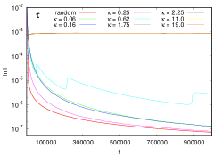
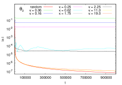
Figure 6: (Left panel) Evolution of $\mathcal{I}$ for $n_{p}=1000$ initial values of $\tau\in(0,1)$ for the map (25) for $\varepsilon=0.05,\mu=10^{-3}\varepsilon$ and eight values of $\omega_{2}^{0}=\kappa\sqrt{3}$. The analytically expected behavior for random motion given by (12) is also included for $N=n_{p}\times t$. (Right panel) Similar to the plot at the left but for the phase $\theta_{2}\in(0,1)$.

Let us now consider the ensemble variance,

$$\langle\Delta H_{2}(t_{j})^{2}\rangle=\frac{1}{n_{p}}\sum_{k=1}^{n_{p}}\left(H_{2}^{(k)}(t_{j})-H_{2}^{(k)}(0)\right)^{2},$$ (26)

where $t_{j}=t_{0}+j\delta t,j\in\mathbb{Z}^{+}$, $\delta t\ll 1$ (see below) being the integration time step of the Hamiltonian (21). We study the temporal evolution of $\langle\Delta H_{2}(t_{j})^{2}\rangle$ over the time span $t=10^{6}$. Fig. 7 presents the evolution of $H_{2}$’s variance for the four smaller values of $\kappa\in K$ where we observe that, within the regarded time interval, the variances increase in mean linearly as expected. Moreover, though the diffusion domains do not overlap, the general properties of the chaotic dynamics provided by $\langle\Delta H_{2}^{2}\rangle$ seems to be quite similar since the variances take nearly the same values. However some departures from the linear trend are noticeable, in particular for $\kappa=0.62$, which are due precisely to phase correlations. The variances for the remainder values of $\kappa$, which are not regarded for the figure, require a much longer time span for any increasing behavior to show up.

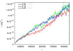
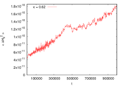
Figure 7: Evolution of $\langle\Delta H_{2}^{2}\rangle$ given in (26) for $\kappa=0.06,0.16,0.25,0.62$ in different panels due to their different scale in the variance. The adopted time-step in this computation is $\delta t=5\times 10^{-4}$

Let us now consider larger values of the parameters, namely, $\varepsilon=0.25$ and $\mu=0.1\varepsilon$, the ones adopted in CGMB17 . In this case the approximation for the relative amplitude $v$ given in (24) presents a maximum $v\approx 1.27$ at $\kappa\approx 0.36$. Thus we consider the following values of $\kappa\in K^{\prime}$:

$$K^{\prime}=\{\kappa:\kappa=0.25,\,0.57,\,0.75,\,1.00,\,1.50,\,2.00,\,9.00\},$$

such that $v$ ranges from $3\times 10^{-18}$ for the larger value of $\kappa$ up to $1.22$ for the smallest one. For the remainder values of $\kappa=0.57,0.75,1.00,1.50,2$ the relative amplitude amounts $1.02,0.66,0.31,4.5\times 10^{-2}$ and $5\times 10^{-3}$ respectively. We observe that for all values of $\kappa$, $v\sim 1$ or smaller and thus $\tau$ should exhibit strong correlations always while it is expected that for the largest values of $\kappa$, $\theta_{2}$ behaves nearly as random, accordingly to the discussion given from the map (25). However, as it is shown in CGMB17 , since both $\varepsilon$ and $\mu$ are comparatively large, resonance interaction is strong leading to large variations of $I_{2}$, $-2\lesssim I_{2}\lesssim 2$ for all values of $\kappa$ (except perhaps for the largest one, see below) and thus the approximations introduced in the derivation of the map seem to be no longer valid, i.e., $\omega_{2}$ could not be regarded as constant and moreover, the motion may be trapped in the resonance $\omega_{2}=0$. Additionally, the resonances $\omega_{1}=0$ and $\omega_{1}=\pm 1$ are close to be in overlap and the amplitude of the resonances $\omega_{1}\pm\omega_{2}=0$ are not negligible, thus around $\omega_{2}=1$ the motion could not be confined to the chaotic layer of the main resonance, as it was discussed in CGMB17 .

[scale=0.6]Arnold_dif_3d_025.eps

Figure 8: Visualization of the diffusion along the chaotic layer of the resonance $\omega_{1}=0$ for $\varepsilon=0.25$ and $\mu=0.1\varepsilon$ and six values of $\kappa\in K^{\prime}$, $0.25$ in red, $0.57$ in green, $0.75$ in blue, $1.00$ in magenta, $1.50$ in cyan and $2.00$ in yellow.

Fig. 8 presents the visualization of the diffusion for the adopted values of $\varepsilon$ and $\mu$ and several initial locations of the ensembles given by $\kappa\in K^{\prime}$. We observe that for $0.25\leq\kappa\leq 1$ the diffusion domains overlap and the action has a significant variation; $-2\lesssim I_{2}\lesssim 2$, while for $\kappa>1$, the diffusion in $I_{2}$ is much more confined, similar to what is observed in Fig. 5. Notice that near $I_{2}=1$ diffusion spreads out of the chaotic layer of the resonance $\omega_{1}=0$ where the motion is under the influence of at least three resonances, $\omega_{1}=0$, $\omega_{1}\pm\omega_{2}=0$ and $\omega_{1}=\pm 1$. Thus, the numerical results confirm that for $\omega_{2}^{0}\lesssim 2$ the map (25) does no longer describe the diffusion along the chaotic layer of the main resonance.

Therefore for these large values of the perturbation parameters we numerically investigate the Hamiltonian (21) instead of the map (25). To this aim, we take an ensemble of $n_{p}=100$ random initial conditions on the separatrix of the resonance $\omega_{1}=0$. We integrate the equations of motion up to $t=5\times 10^{5}$ with a small time step $\delta t=5\times 10^{-4}$ and take the values of $\theta_{2}$ and $t\equiv\tau$ each time $|\theta_{1}-\pi|\leq 0.001$, avoiding two consecutive crossings of the surface $\theta_{1}=\pi$ by a single trajectory. After normalizing $\theta_{2}$ and $\tau$ to the unit interval, on adopting a sample time interval $\Delta t=500$ and setting $q=10^{3}$, we compute the information (11) for the seven values of $\omega_{2}^{0}=\kappa\sqrt{3}$, with $\kappa\in K^{\prime}$.

For the theoretical estimates, the total number of points is now $N=n_{p}\times t/\delta t$, but since we are considering only those satisfying $|\theta_{1}-\pi|\leq 0.001$, we set $N=\beta n_{p}\times t/\delta t$, with $\beta\ll 1$, and therefore (12) and (16) become

$$\mathcal{I}(\gamma_{x}^{r},\alpha)\approx\frac{q\delta t}{2\beta n_{p}\ln q}\frac{1}{t},\qquad\mathcal{I}(\gamma_{x}^{s},\alpha)\approx\frac{q^{2}\delta t^{2}}{8\beta^{2}\ln q}\frac{1}{t^{2}},$$ (27)

respectively, where $\beta\approx 3\times 10^{-4}$ obtained numerically.

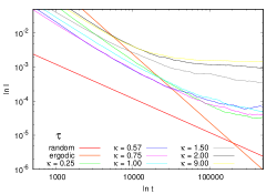
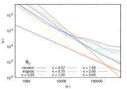
Figure 9: (Left panel) Evolution of $\mathcal{I}$ for the phase $\tau\in(0,1)$ corresponding to the values of $t$ when the the pendulum crosses the surface $\theta_{1}=\pi$ for $n_{p}=100$ random initial values on the separatrix of the resonance $\omega_{1}=0$ for the Hamiltonian (21) with $\varepsilon=0.25,\mu=0.1\varepsilon$ and seven values of $\omega_{2}^{0}=\kappa\sqrt{3}$. The analytical expected behavior for random and ergodic motion given by (27) are also included for $N=\beta n_{p}\times t/\delta t$, with $\beta\approx 3\times 10^{-4}$. (Right panel) Similar to the plot at the left but for the phase $\theta_{2}\in(0,1)$.

Fig. 9 shows the results for $\mathcal{I}$ for all the ensembles defined by $\omega_{2}^{0}=\sqrt{3}\kappa$, with $\kappa\in K^{\prime}$. It becomes evident that in any case, the phase $\tau$ is always correlated, though up to $t\approx 10^{4}$ $\mathcal{I}$ decreases with a power law near to $t^{-1}$, at larger times decreases in a much slower way and for large $\kappa$ it reaches a nearly constant value at relatively short times. On the other hand, while $\theta_{2}$ decreases with time for all ensembles, it could be assumed nearly random only for large values of $\omega_{2}$, precisely when $\omega_{2}\approx\mathrm{const}$ is a rough approximation. We observe that up to $t\approx 2\times 10^{4}$ it is $\mathcal{I}\sim t^{p}$ with $-2<p<-1$, but for larger times only those ensembles located at large $\omega_{2}^{0}$, $\mathcal{I}\sim t^{-1}$. Note that for $\kappa=9.00$, $\mathcal{I}$ behaves initially in an ergodic rather than random fashion, as expected since $\theta_{2}\approx\omega_{2}t$.

In CGMB17 as well as in GC18 it was shown that for $\varepsilon=0.25$ and $\mu=0.1\varepsilon$, the evolution of the ensemble variance (26) for $|\omega_{2}^{0}|<2$ reveals that the diffusion is clearly anomalous, in particular a sub-diffusive process. This fact motivated our introducing an alternative way of measuring both the extent and the rate of the diffusion in GC18 , namely by means of the Shannon entropy.

Regarding the diffusion observed in $I_{2}$, we can say that for $\omega_{2}\lesssim 1$, the diffusion is certainly driven by all first order resonances and it has no sense to speak about layer or driving resonances, all of them contributing to the motion along and across the chaotic layer of the guiding resonance. On the other hand, for $\omega_{2}\gg 1$ Chirikov’s description could apply, resonance interaction is weak so the assumptions beneath the map (25) become plausible, the amplitude being $v\ll 1$ and regarding the evolution of $\theta_{2}$ for large $\omega_{2}$ we could take $\langle\cos^{2}\theta_{2}\rangle\approx Rt/2$ with $R\lesssim 1$.

Let us mention that in case of a general multidimensional Hamiltonian, Chirikov derived a similar map than (25) but involving several phases and the discussion about the behavior of the different phases is quite similar to the one given above (see Ch79 , C02 , CEGM14 ).

4 Discussion

Herein we have shown that the Shannon entropy turns out to be a rather simple and effective way to measure phase correlations. Even though we apply this technique to area–preserving maps or near–integrable Hamiltonian systems, its formulation –given in Section 2– reveals that it can be used in a wide range of problems beyond dynamical systems. The numerical experiments included therein unfold that the derived analytical estimates for absence of correlations or ergodicity are quite accurate.

The numerical simulations presented in this work concern in general chaotic motion, thus a given phase variable cover completely the unit interval. Therefore, the key point in the present approach is the probability of occupation of each element of the partition, $\mu(a_{k})=n_{k}/N$. If the $n_{k}$ are randomly distributed, thus the information $\mathcal{I}$ decreases as the inverse of the integer time or total number of phase values. On the other hand, if the $n_{k}$ have a uniform distribution, then the information decreases faster, following an inverse square law. Any other dependence of $\mathcal{I}$ with $N$ reveals the existence of correlations among the phase values. Therefore a reference level for the information could be adopted for a given distribution of $N$ values of the phases, in order to discriminate between strong and weak correlations in the sample.

In dynamical systems like those studied in Section 3, it would be much more interesting to study how the information evolves with time. In such a way it is possible to reveal and understand the underlying dynamics, as for instance in Figs. 3 and 4.

More interesting is the use of this novel tool to revisit Chirikov’s approach to diffusion along the chaotic layer of a single resonance or Arnold diffusion, in a broad sense of this term. We succeed in revealing strong and weak correlations that prevent the free diffusion and therefore the so–called reduced stochasticity approximation, in the sense that $\langle\cos^{2}\theta_{2}\rangle\approx Rt/2$ or $\langle\sin^{2}\tau\rangle\approx Rt/2$ with $R<1$ is not applicable and thus the obtained estimates for the diffusion coefficient are not correct (see Ch79 –Section 7, CGMB17 for more details). Particularly, the map (25) could be a reliable model to investigate diffusion along the chaotic layer of resonance $\omega_{1}=0$ provided that $\mu\varepsilon\ll\varepsilon\ll 1$ and $\omega_{2}$ is far away from $0$ and $1$ as Fig. 6 shows. On the other hand, if the parameters are not too small, the map would provide a fair approximation to the diffusion that actually takes place only if $\omega_{2}\gg 1$. In other words, Chirikov’s formulation seems to be adequate when the diffusion extent is quite restricted and thus it makes sense to derive a local diffusion coefficient.

Conflict of interest

The authors declare that they have no conflict of interest.

References

- (1) Arnold, V. I., On the nonstability of dynamical systems with many degrees of freedom, Soviet Mathematical Doklady 5, 581-585 (1964)
- (2) Arnol’d, V., Avez, A. Ergodic Problems of Classical Mechanics, 2nd. Ed. (Addison-Wesley, New York), (1989)
- (3) Berne, B.J.,Harp, G.D. On the Calculation of Time Correlation Functions in I. Prigogine, Stuart A. Rice eds., Advance in Chemical Physics, Vol XVII (1970)
- (4) Chirikov, B. V., Institute of Nuclear Physics, Novosibirsk (in Russian), Preprint 267, (1969), Engl. Transl., CERN Trans. 71 - 40, Geneva, October (1971)
- (5) Chirikov, B. V., A Universal instability of many-dimensional oscillator systems, Physics Reports, 52, 263 (1979)
- (6) Cincotta, P. M., Helmi, A., Méndez, M., Núñez, J. A., Vucetich, H., Astronomical time-series analysis -II. A search for periodicity using the Shannon entropy, Monthly Notices of the Royal Astronomical Society, 302, 582 (1999)
- (7) Cincotta, P. M., Astronomical time-series analysis -III. The role of the observational errors in the minimum entropy method, Monthly Notices of the Royal Astronomical Society, 307, 941 (1999)
- (8) Cincotta, P. M., Arnold diffusion: an overview through dynamical astronomy, New Astronomy Reviews, 46, 13-39 (2002)
- (9) Cincotta, P. M., Efthymiopoulos, C., Giordano, C. M., Mestre, M. F., Chirikov and Nekhoroshev diffusion estimates: bridging the two sides of the river, Physica D, 266, 49 (2014)
- (10) Cincotta, P. M., Giordano, C. M., Martí, J. G., Beaugé, C., On the chaotic diffusion in multidimensional Hamiltonian systems, Celestial Mechanics and Dynamical Astronomy, 130 article id. (2018)
- (11) Chandler, D., Introduction to Modern Statistical Mechanics, (New York: Oxford University Press), (1987)
- (12) Efthymiopoulos, C., Harsoula, M., The speed of Arnold diffusion, Physica D, 251, 19 (2013)
- (13) Froeschlé, C., Guzzo, M., Lega, E., Local and global diffusion along resonant lines in discrete quasi-integrable dynamical systems Celestial Mechanics and Dynamical Astronomy, 92, 243 (2005)
- (14) Froeschlé, C., Lega, E., Guzzo, M., Analysis of the chaotic behavior of orbits diffusing along the Arnold web, Celestial Mechanics and Dynamical Astronomy, 95, 141 (2006)
- (15) Giordano, C.M, Cincotta, P.M., The Shannon entropy as a measure of diffusion in multidimensional dynamical systems, CMDA 130, article id. N (2018)
- (16) Guzzo, M., Lega, E., Froechlé, C., First numerical evidence of global Arnold diffusion in quasi–integrable systems Discrete and Ccontinuous Dynamical Systems B 5, 687 (2005)
- (17) Katz, A., Principles of Statistical Mechanics, The Information Theory Approach, (San Francisco: W.H. Freeman & Co.), (1967)
- (18) Klafter, J., Blumen, A., Zumofen, G., Shlesinger, M., Lévy walk approach to anomalous diffusion, Physica A, 168, 637 (1990)
- (19) Klafter, J., Zumofen, G., Shlesinger, M., Lévy walks in dynamical systems, Physica A, 200, 222 (1993)
- (20) Korabel, N., Klages, R., Microscopic chaos and transport in many-particle systems, Physica D, 187, 66 (2004).
- (21) Lega, E., Froeschlé, C., Guzzo, Diffusion in Hamiltonian quasi-integrable systems, Lecture Notes in Physics, 729, 29 (2008)
- (22) Lega, E., Guzzo, M., Froeschlé, C., Detection of Arnold diffusion in Hamiltonian systems, Physica D, 182, 179 (2003)
- (23) Lesne, A., Shannon entropy: a rigorous notion at the crossroads between probability, information theory, dynamical systems and statistical physics, Mathematical Structures in Computer Science, 24, e240311, doi:10.1017/S0960129512000783 (2014)
- (24) Maffione, N. P., Gómez F. A., Cincotta, P. M.,Giordano, C. M., Cooper, A. P., O’ Shea, B.W., On the relevance of chaos for halo stars in the solar neighbourhood, Monthly Notices of the Royal Astronomical Society, 453, 2830 (2015)
- (25) Maffione, N. P., Gómez F. A., Cincotta, P. M.,Giordano, C. M., Grand, R., Marinacci, F., Pakmor, R., Simpson, C., Springel, V., Frenk, C., On the relevance of chaos for halo stars in the solar neighbourhood II, Monthly Notices of the Royal Astronomical Society, 478, 4052 (2018)
- (26) Martí, J. G.; Cincotta, P. M.; Beaugé, C. Chaotic diffusion in the Gliese-876 planetary system, Monthly Notices of the Royal Astronomical Society, 460, 1094 (2016)
- (27) Miguel, N, Simó, C, Vieiro, A., On the effect of islands in the diffusive properties of the standard map, for large parameter values, Foundations of Computational Mathematics, 15, 89 (2014)
- (28) Reichl, L.E., A Modern Course in Statistical Physics, (New York: Wiley-Interscience), 1998.
- (29) Shannon, C., Weaver, W., The Mathematical Theory of Communication, (Urbana: Illinois U.P.), (1949)
- (30) Schwarzl, M., Godec, A., Metzler, R., Quantifying non-ergodicity of anomalous diffusion with higher order moments, Scientific Reports, 7, doi:10.1038/s41598-017-03712-x (2017)
- (31) Venegeroles, R. Calculation of superdiffusion for the Chirikov-Taylor model, Physical Review Letters, 101, 54102 (2008)
- (32) Wehrl, A., General properties of entropy, Review of Modern Physics, 50, 2, 221 (1978)
- (33) Zaslavsky, G. M., Fractional kinetic equation for Hamiltonian chaos, Physica D, 76, 110 (1994)
- (34) Zaslavsky, G. M., Abdullaev, S.S., Scaling properties and anomalous transport of particles inside the stochastic layer, Physical Review E, 51, 3901, 1995
- (35) Zaslavsky, G. M., Edelman, M., Niyazow, B. A., Self-similarity, renormalization, and phase space nonuniformity of Hamiltonian chaotic dynamics, Chaos, 7, 159, (1997)
- (36) Zaslavsky, G. M., Niyazow, B. A., Fractional kinetics and accelerator modes, Physics Reports, 283, 73 (1997)
- (37) Zaslavsky, G. M., Edelman, M., Hierarchical structures in the phase space and fractional kinetics: I. Classical systems, Chaos, 10, 135 (2000)
- (38) Zaslavsky, G. M. Chaos, fractional kinetics, and anomalous transport Physics Reports, 371, 461 (2002)