Supplementary Information “Experimental repetitive quantum channel simulation”

I Experimental System and Setup

Our experimental device is measured in a dilution refrigerator with a base temperature of about 10 mK. The device consists of an ancillary transmon qubit dispersively coupled to both a readout cavity and a storage cavity. The ancilla qubit is fabricated on a $c$-plane sapphire (Al₂O₃) substrate with the standard double-angle evaporation of aluminum and electron-beam lithography. The rectangular cavities are made of high purity 5N5 aluminum, chemically etched for a better coherence time Reagor et al. (2013, 2016). The ancillary transmon qubit has a frequency $\omega_{\mathrm{q}}/2\pi=5.692$ GHz, an energy relaxation time $T_{1}=30~{}{\mathrm{\mu}}$s, and a pure phasing time $T_{\phi}=120~{}{\mathrm{\mu}}$s. The storage cavity has a frequency $\omega_{\mathrm{s}}/2\pi=7.634$ GHz, a single-photon lifetime $T_{1}^{\mathrm{s}}=143~{}{\mathrm{\mu}}$s, and a coherence time $T_{2}^{\mathrm{s}}=250~{}{\mathrm{\mu}}$s. Fock states $\left|0\right\rangle$ and $\left|1\right\rangle$ of the storage cavity constitute the two bases of a photonic qubit on which channel simulations are realized. The dephasing, damping, and arbitrary channels all rely on the dispersive interaction $\chi_{\mathrm{s}}/2\pi=1.90$ MHz between the ancilla and the photonic qubit. The readout cavity is at a frequency of $\omega_{\mathrm{r}}/2\pi=8.610$ GHz, and has a lifetime of 44 ns and a dispersive interaction $\chi_{\mathrm{r}}/2\pi=3.65$ MHz with the ancilla. With the help of a Josephson parametric Amplifier (JPA) Hatridge et al. (2011); Roy et al. (2015); Kamal et al. (2009); Murch et al. (2013) as the first stage of amplification, quantum non-demolition single-shot measurements of the ancilla qubit can be realized with high fidelities: $>99.9\%$ for the ground state $\left|g\right\rangle$ and $98.9\%$ for the excited state $\left|e\right\rangle$ in a duration of 320 ns. Therefore, each readout measurement throughout our experiment returns a digitized value of the ancilla qubit state.

Fast real-time adaptive control is vital for the demonstrated channel simulations. This is achieved through three field programmable gate arrays (FPGA) with home-made logics, which are able to integrate readout signal sampling, ancilla state estimation, and manipulation signal generation together, and also allow us to individually control the ancilla qubit, the photonic qubit, and the readout cavity. The latency time, defined as the time interval between sending out the last point of the readout signal and sending out the first point of the control signal, is 340 ns (about $1\%$ of the ancilla qubit lifetime). This time includes the signal travel time through the whole experimental circuitry. More details of the experimental setup and FPGAs can be found in our earlier report in Ref. Hu et al., 2018.

II General Theory

II.1 Quantum channel and process matrix

The Kraus representation of a quantum channel or quantum operation can be written as Nielsen and Chuang (2000)

$$\rho\mapsto\mathcal{E}\left(\rho\right)=\sum_{k=1}^{M}E_{k}\rho E_{k}^{\dagger},$$ (S.1)

with $1\leq M\leq d^{2}$ ($d$ is the Hilbert space dimension) and the Kraus operators satisfy

$$\sum_{k}E_{k}^{\dagger}E_{k}=\mathbf{I},$$ (S.2)

where $\mathbf{I}$ is the unity matrix.

Representing the Kraus operators in a certain basis, the channel can also be expressed based on the process $\chi$ matrix Bhandari and Peters (2016)

$$\rho\mapsto\sum_{m,n}\chi_{mn}\widetilde{E_{m}}\rho\widetilde{E_{n}}^{\dagger},$$ (S.3)

where the $\chi$ matrix contains $d^{4}-d^{2}$ independent parameters under the constraints that

$$\sum_{m,n}\chi_{mn}\widetilde{E_{n}}^{\dagger}\widetilde{E_{m}}=\mathbf{I}.$$ (S.4)

Usually, we choose Pauli matrices as the operation elements, with the definition consistent with those in Nielsen and Chuang (2000):

$$\widetilde{E_{m}}\in\left\{\mathbf{I},\mathbf{X},-i\mathbf{Y},\mathbf{Z}\right\}$$ (S.5)

with

$$\mathbf{X}=\left[\begin{array}[]{cc}0&1\\ 1&0\end{array}\right],\,\mathbf{Y}=\left[\begin{array}[]{cc}0&-i\\ i&0\end{array}\right],\,\mathbf{Z}=\left[\begin{array}[]{cc}1&0\\ 0&-1\end{array}\right],$$ (S.6)

and the quantum state $\alpha\left|0\right\rangle+\beta\left|1\right\rangle$ is written in a vector notation as

$$\left[\begin{array}[]{c}\alpha\\ \beta\end{array}\right].$$ (S.7)

In the following, we provide details of the basic channels studied in this work.

II.1.1 Identity channel

The identity channel is trivial:

$$\mathcal{E}\left(\rho\right)=\rho,$$ (S.8)

and the corresponding process matrix is

$$\chi_{\mathrm{I}}=\left[\begin{array}[]{cccc}1&0&0&0\\ 0&0&0&0\\ 0&0&0&0\\ 0&0&0&0\end{array}\right].$$ (S.9)

To characterize the ability of quantum channel $\chi$ for keeping quantum information, we introduce the process fidelity as

$$F_{\chi}=\mathrm{Tr}\left(\chi_{\mathrm{I}}\chi\right)$$ (S.10)

II.1.2 Depolarization channel

The depolarization channel is defined as Nielsen and Chuang (2000)

$$\mathcal{E}\left(\rho\right)=\left(1-p\right)\mathbf{I}\rho\mathbf{I}+\frac{p}{3}\left(\mathbf{X}\rho\mathbf{X}+\mathbf{Y}\rho\mathbf{Y}+\mathbf{Z}\rho\mathbf{Z}\right),$$ (S.11)

and the corresponding process matrix is

$$\chi_{\mathrm{dpl}}=\left[\begin{array}[]{cccc}1-p&0&0&0\\ 0&\frac{p}{3}&0&0\\ 0&0&\frac{p}{3}&0\\ 0&0&0&\frac{p}{3}\end{array}\right].$$ (S.12)

The effect of this channel is to mix the input state with the completely mixed state $\mathbf{I}/2$.

II.1.3 Qubit dephasing channel

The dephasing channel is defined as Nielsen and Chuang (2000)

$$\mathcal{E}\left(\rho\right)=E_{0}\rho E_{0}^{\dagger}+E_{1}\rho E_{1}^{\dagger}$$ (S.13)

with

$$E_{0}=\sqrt{p}\mathbf{I},\,E_{1}=\sqrt{1-p}\mathbf{Z},$$ (S.14)

where $p\in\left[0,1\right]$. According to Eq. (S.3), we can get the $\chi$ matrix for a dephasing channel as

$$\chi_{\mathrm{dph}}=\left[\begin{array}[]{cccc}p&0&0&0\\ 0&0&0&0\\ 0&0&0&0\\ 0&0&0&1-p\end{array}\right].$$ (S.15)

After repetitively implementing the channel for $n$ times, we have the process matrix for $\mathcal{E}^{n}$

$$\chi_{\mathrm{dph}}^{\left(n\right)}=\left[\begin{array}[]{cccc}2^{n-1}(p-\frac{1}{2})^{n}+\frac{1}{2}&0&0&0\\ 0&0&0&0\\ 0&0&0&0\\ 0&0&0&\frac{1}{2}-2^{n-1}(p-\frac{1}{2})^{n}\end{array}\right].$$ (S.16)

Therefore, the process fidelity decays exponentially with $n$ as

$$F_{\chi}=\frac{1}{2}\left[1+\left(2p-1\right)^{n}\right],$$ (S.17)

which converges to $F_{\chi}=\frac{1}{2}$ for $n\gg 1$.

II.1.4 Qubit damping channel

The amplitude damping channel is defined as Nielsen and Chuang (2000)

$$\mathcal{E}\left(\rho\right)=E_{0}\rho E_{0}^{\dagger}+E_{1}\rho E_{1}^{\dagger},$$ (S.18)

with

$$E_{0}=\left[\begin{array}[]{cc}1&0\\ 0&\sqrt{1-\gamma}\end{array}\right],\,E_{1}=\left[\begin{matrix}0&\sqrt{\gamma}\\ 0&0\end{matrix}\right],$$ (S.21)

where $\gamma\in\left[0,1\right]$. According to Eq. (S.3), we can get the $\chi$ matrix for a damping channel

$$\chi_{{\rm dmp}}=\left[\begin{array}[]{cccc}\frac{\sqrt{1-\gamma}}{2}-\frac{\gamma}{4}+\frac{1}{2}&0&0&\frac{\gamma}{4}\\ 0&\frac{\gamma}{4}&-\frac{\gamma}{4}&0\\ 0&-\frac{\gamma}{4}&\frac{\gamma}{4}&0\\ \frac{\gamma}{4}&0&0&\frac{1}{2}-\frac{\sqrt{1-\gamma}}{2}-\frac{\gamma}{4}\end{array}\right].$$ (S.22)

After repetitively implementing the channel for $n$ times, we have the process matrix for $\mathcal{E}^{n}$

$$\chi_{{\rm dmp}}^{\left(n\right)}=\left[\begin{array}[]{cccc}\frac{[1+(1-\gamma)^{\frac{n}{2}}]^{2}}{4}&0&0&\frac{[1-(1-\gamma)^{n}]}{4}\\ 0&\frac{[1-(1-\gamma)^{n}]}{4}&-\frac{[1-(1-\gamma)^{n}]}{4}&0\\ 0&-\frac{[1-(1-\gamma)^{n}]}{4}&\frac{[1-(1-\gamma)^{n}]}{4}&0\\ \frac{[1-(1-\gamma)^{n}]}{4}&0&0&\frac{[1-(1-\gamma)^{\frac{n}{2}}]^{2}}{4}\end{array}\right].$$ (S.23)

Therefore, the process fidelity decays bi-exponentially with $n$ as

$$F_{\chi}=\frac{1}{4}+\frac{1}{2}(1-\gamma)^{\frac{n}{2}}+\frac{1}{4}(1-\gamma)^{n},$$ (S.24)

which converges to $F_{\chi}=\frac{1}{4}$ for $n\gg 1$.

II.2 Correspondence between quantum channel simulation and master equation

II.2.1 Liouvillian and repetitive quantum channel simulation

Here, we explain the correspondence between digital quantum channel simulation and master equation for continuous open system dynamics. We start the discussion with a simple example, in which the system couples to a Markovian environment through the operator $o$ as

$$H=H_{0}+\sum_{\omega}\omega b_{\omega}^{\dagger}b_{\omega}+\sum_{\omega}\left(g_{\omega}o^{\dagger}b_{\omega}+h.c.\right),$$ (S.25)

where the bosonic operator $b_{\omega}$ denotes the harmonic oscillator mode in the bath with frequency of $\omega$, and $g_{\omega}$ is the corresponding coupling strength. Applying the Born approximation, we obtain the evolution of the system density matrix as Carmichael (2003)

$$\frac{d}{dt}\rho_{\mathrm{s}} = -i\left[H_{0},\rho_{\mathrm{s}}\right]$$ (S.26)

$$-\left\{\int_{0}^{t}d\tau\left[oo^{\dagger}\rho_{\mathrm{s}}\left(t-\tau\right)-o^{\dagger}\rho_{\mathrm{s}}\left(t-\tau\right)o\right]\sum_{\omega}\left|g_{\omega}^{2}\right|\left\langle b_{\omega}^{\dagger}\left(t\right)b_{\omega}\left(t-\tau\right)\right\rangle+h.c.\right\}$$

$$-\left\{\int_{0}^{t}d\tau\left[o^{\dagger}o\rho_{\mathrm{s}}\left(t-\tau\right)-o\rho_{\mathrm{s}}\left(t-\tau\right)o^{\dagger}\right]\sum_{\omega}\left|g_{\omega}^{2}\right|\left\langle b_{\omega}\left(t\right)b_{\omega}^{\dagger}\left(t-\tau\right)\right\rangle+h.c.\right\}.$$

For a low-temperature reservoir, $\left\langle b_{\omega}^{\dagger}\left(t\right)b_{\omega}\left(t-\tau\right)\right\rangle\approx 0$ and $\left\langle b_{\omega}\left(t\right)b_{\omega}^{\dagger}\left(t-\tau\right)\right\rangle=\delta\left(\tau\right)$. If we define $\kappa=\frac{1}{2}\int d\omega\xi\left(\omega\right)\left|g_{\omega}^{2}\right|$ with $\xi\left(\omega\right)$ being the density of states in the bath, we obtain the master equation in the Lindblad form as Petruccione and Breuer (2002); Gardiner et al. (2004)

$$\frac{d}{dt}\rho =-i\left[H_{0},\rho\right]+\kappa\left(2o\rho o^{\dagger}-o^{\dagger}o\rho-\rho o^{\dagger}o\right)$$ (S.27)

$$=\mathcal{L}_{0}\left(\rho\right)+\mathcal{L}_{1}\left(\rho\right),$$ (S.28)

with Liouvillian $\mathcal{L}_{0}$ and $\mathcal{L}_{1}$ describing the coherent and incoherent evolutions, respectively. For $dt\rightarrow 0$, we have

$$\rho\left(t+dt\right)-\rho\left(t\right) =\mathcal{L}_{0}\left(\rho\right)dt+\mathcal{L}_{1}\left(\rho\right)dt+\mathcal{O}\left[\left(H_{0}dt\right)^{2}\rho\right]+\mathcal{O}\left[\left(\kappa dt\right)^{2}\rho\right].$$ (S.29)

Through channel simulation, we can implement unitary channel

$$\mathcal{E}_{0}\left(\rho\right) =e^{-iHdt}\rho e^{iHdt}$$ (S.30)

$$=\rho-i\left[H_{0}dt,\rho\right]+\mathcal{O}\left[\left(H_{0}dt\right)^{2}\rho\right]$$ (S.31)

$$=\rho+\mathcal{L}_{0}\left(\rho\right)dt+\mathcal{O}\left[\left(H_{0}dt\right)^{2}\rho\right]$$ (S.32)

through arbitrary unitary control Krastanov et al. (2015), and non-unitary channel

$$\mathcal{E}_{1}\left(\rho\right) =E_{1,0}\rho E_{1,0}^{\dagger}+E_{1,1}\rho E_{1,1}^{\dagger}$$ (S.33)

$$=\rho+\kappa dt\left(2o\rho o^{\dagger}-o^{\dagger}o\rho-\rho o^{\dagger}o\right)+\mathcal{O}\left[\left(\kappa dt\right)^{2}\rho\right]$$ (S.34)

$$=\mathcal{L}_{1}\left(\rho\right)dt+\mathcal{O}\left[\left(\kappa dt\right)^{2}\rho\right]$$ (S.35)

with

$$E_{1,0} =\sqrt{2\kappa dt}o,$$ (S.36)

$$E_{1,1} =\mathbf{I}-\kappa dto^{\dagger}o.$$ (S.37)

Therefore, by sequentially implementing these two channels

$$\mathcal{E}_{1}\circ\mathcal{E}_{0}\left(\rho\right) =\mathcal{L}_{0}\left(\rho\right)dt+\mathcal{L}_{1}\left(\rho\right)dt+\mathcal{O}\left[\left(H_{0}dt\right)^{2}\rho\right]+\mathcal{O}\left[\left(\kappa dt\right)^{2}\rho\right]$$ (S.38)

$$\approx e^{dt\left(\mathcal{L}_{0}+\mathcal{L}_{1}\right)}\rho,$$ (S.39)

we obtain the effective implementation of the Liouvillian with an error to the order of $\left(H_{0}dt\right)^{2}+\left(\kappa dt\right)^{2}$.

The above derivations can be easily generalized to multiple-Liouvillian case, i.e. $\sum_{j}\mathcal{L}_{j}$. As proved in Refs. Kliesch et al. (2011); Sweke et al. (2014), the effective continuous open quantum system dynamics can be realized by repetitively implementing the quantum channels which correspond to each individual Liouvillian alternatively.

II.2.2 Qubit dephasing channel

When $o=\mathbf{Z}$ and $H=0$ in Eq. (S.27), the master equation corresponds to a simple Markovian dephasing channel on a qubit. According to the analysis above, when

$$E_{1,0} =\sqrt{2\kappa dt}\mathbf{Z},$$ (S.40)

$$E_{1,1} =\sqrt{1-2\kappa dt}\mathbf{I},$$ (S.41)

the repetitive implementation of the channel (in the limit of $\kappa dt\ll 1$) will give us an effective continuous dephasing process. According to the definition of a dephasing channel (Eq. (S.13)), it requires that $p=1-2\kappa dt$. It also indicates that the implementation of the digital dephasing channel simulation with $1-p\ll 1$ and a duration of $\tau_{0}$ leads to an effective continuous dephasing Liouvillian with a dephasing rate $\kappa=\left(1-p\right)/2\tau_{0}$, and the corresponding phase coherence time is $T_{2}=1/4\kappa$.

II.2.3 Qubit damping channel

Similarly, when

$$o=\sigma_{-}=\left[\begin{array}[]{cc}0&1\\ 0&0\end{array}\right]$$ (S.42)

and $H=0$ in Eq. (S.27), the master equation corresponds to a simple Markovian excited state damping channel on a qubit. If

$$E_{1,0} =\sqrt{2\kappa dt}\sigma_{-},$$ (S.43)

$$E_{1,1} =\mathbf{I}-\kappa dt\frac{\mathbf{I}-\mathbf{Z}}{2},$$ (S.44)

the repetitive implementation of the channel (in the limit of $\kappa dt\ll 1$) will give us an effective continuous damping process. According to the definition of a damping channel Eq. (S.21), it requires that $\gamma=2\kappa dt$. It also indicates that the implementation of the digital damping channel simulation with $\gamma\ll 1$ and a duration of $\tau_{0}$ leads to an effective continuous damping Liouvillian with a damping rate $\kappa=\gamma/2\tau_{0}$.

III Experimental Quantum Channel Simulations

III.1 The dephasing channel simulation

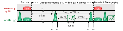
Figure S1: Experimental sequence for a dephasing channel simulation. Density matrices at the arrows are shown in detail in the text.

In our experiment, the dephasing channel is realized by using the control pulse sequence in Fig. 2(a) in the main text. To explain the protocol, we analyze the procedures in detail as follows.

1. The ancilla qubit is initialized to the ground state $\rho_{\mathrm{a}}=\left|g\right\rangle\left\langle g\right|$, and the photonic qubit is encoded in $\rho_{\mathrm{in}}$. Then the input of the system is

   $$\rho_{0}=\rho_{\mathrm{a}}\otimes\rho_{{\rm in}}=\left[\begin{array}[]{cc}1&0\\ 0&0\end{array}\right]\otimes\left[\begin{array}[]{cc}a&b\\ c&d\end{array}\right].$$ (S.45)

2. After applying $X_{\theta}$ (a unitary operation $U_{X}\left(\theta\right)=e^{-i\frac{\theta}{2}\mathbf{X}}$) to the ancilla qubit, we have

   $$\rho_{0}\mapsto\rho_{1} =U_{\mathbf{X}}\left(\theta\right)\rho_{0}U_{\mathbf{X}}^{\dagger}\left(\theta\right)$$ (S.46)

   $$=\left[\begin{array}[]{cc}\cos^{2}\left(\frac{\theta}{2}\right)&i\sin\left(\frac{\theta}{2}\right)\cos\left(\frac{\theta}{2}\right)\\ -i\sin\left(\frac{\theta}{2}\right)\cos\left(\frac{\theta}{2}\right)&\sin^{2}\left(\frac{\theta}{2}\right)\end{array}\right]\otimes\left[\begin{array}[]{cc}a&b\\ c&d\end{array}\right].$$ (S.51)

3. According to the Hamiltonian $H=\omega_{s}a^{\dagger}a+\omega_{a}|e\rangle\langle e|-\chi_{{\rm{s}}}a^{\dagger}a|e\rangle\langle e|$, the $\left|e\right\rangle\left|1\right\rangle$ state gains an extra phase $e^{i\chi_{{\rm{s}}}t}$ for a duration of $t$. Thus, waiting for a duration of $t=3\pi/\chi_{{\rm{s}}}$, a controlled-Z (CZ) gate between the ancilla and the photonic qubit can be realized as

   $$\rho_{1}\mapsto\rho_{2} =U_{\mathrm{CZ}}\rho_{1}U_{\mathrm{CZ}}^{\dagger}$$ (S.52)

   $$=\left[\begin{array}[]{cc}\cos^{2}\left(\frac{\theta}{2}\right)\left[\begin{array}[]{cc}a&b\\ c&d\end{array}\right]&i\sin\left(\frac{\theta}{2}\right)\cos\left(\frac{\theta}{2}\right)\left[\begin{array}[]{cc}a&-b\\ c&-d\end{array}\right]\\ -i\sin\left(\frac{\theta}{2}\right)\cos\left(\frac{\theta}{2}\right)\left[\begin{array}[]{cc}a&b\\ -c&-d\end{array}\right]&\sin^{2}\left(\frac{\theta}{2}\right)\left[\begin{array}[]{cc}a&-b\\ -c&d\end{array}\right]\end{array}\right].$$ (S.63)

4. When tracing out the ancilla qubit state, we have the output state of the photonic qubit as

   $$\rho_{\mathrm{out}} =\mathrm{Tr}_{\mathrm{a}}\left(\rho_{2}\right)$$ (S.64)

   $$=\cos^{2}\left(\frac{\theta}{2}\right)\left[\begin{array}[]{cc}a&b\\ c&d\end{array}\right]+\sin^{2}\left(\frac{\theta}{2}\right)\left[\begin{array}[]{cc}a&-b\\ -c&d\end{array}\right]$$ (S.69)

   $$=\left[\begin{array}[]{cc}a&b{\rm cos}\left(\theta\right)\\ c{\rm cos}\left(\theta\right)&d\end{array}\right].$$ (S.72)

5. To discard the ancilla qubit state, the ancilla is measured after the CZ gate and a conditional $X$ operation is implemented when the measurement outcome is $\left|e\right\rangle$. This measurement and adaptive operation on the ancilla qubit can be described as

   $$\mathcal{E}_{\mathrm{MF}}\left(\rho_{\mathrm{a}}\right):\,\rho_{\mathrm{a}}\mapsto\left|g\right\rangle\left\langle g\right|\rho_{\mathrm{a}}\left|g\right\rangle\left\langle g\right|+X\left|e\right\rangle\left\langle e\right|\rho_{\mathrm{a}}\left|e\right\rangle\left\langle e\right|X^{\dagger},$$ (S.73)

   i.e.

   $$\mathcal{E}_{\mathrm{MF}}\left(\rho_{\mathrm{a}}\right):\,\rho_{\mathrm{a}}\mapsto\left[\begin{array}[]{cc}1&0\\ 0&0\end{array}\right]\mathrm{Tr}_{\mathrm{a}}\left(\rho_{\mathrm{a}}\right).$$ (S.74)

   Thus, the system state before decoding is

   $$\rho_{2}\mapsto\rho_{3} =\mathcal{E}_{\mathrm{MF}}\left(\rho_{2}\right)=\left[\begin{array}[]{cc}1&0\\ 0&0\end{array}\right]\otimes\mathrm{Tr}_{\mathrm{a}}\left(\rho_{2}\right).$$ (S.77)

   $$=\left[\begin{array}[]{cc}1&0\\ 0&0\end{array}\right]\otimes\left[\begin{array}[]{cc}a&b{\rm cos}\left(\theta\right)\\ c{\rm cos}\left(\theta\right)&d\end{array}\right].$$ (S.82)

Comparing the input and output of the experimental procedure, we find the obtained channel is

$$\mathcal{E}_{\mathrm{anc}\otimes\mathrm{target}}=\mathcal{I}_{\mathrm{anc}}\otimes\mathcal{E}_{\mathrm{target}},$$ (S.83)

where $\mathcal{I}:\,\rho\mapsto\rho$ is the identity channel and

$$\mathcal{E}_{\mathrm{target}}:\,\rho\mapsto\cos^{2}\left(\frac{\theta}{2}\right)\mathbf{I}\rho\mathbf{I}^{\dagger}+\sin^{2}\left(\frac{\theta}{2}\right)\mathbf{Z}\rho\mathbf{Z}^{\dagger}.$$ (S.84)

According to the definition in last section [Eq. (S.13)], the dephasing channel with $p=\cos^{2}\left(\frac{\theta}{2}\right)$ is realized.

The effects of the repetitive dephasing channel simulation and the intrinsic decoherence can simply be added together, which leads to an effective channel coherence time

$$\frac{1}{T_{2}^{c}}=-\frac{{\rm ln}\left(2\cos^{2}\frac{\theta}{2}-1\right)}{\tau_{0}}+\frac{1}{T_{2}^{0}},$$ (S.85)

where $T_{2}^{0}$ is the intrinsic coherence time (when $\theta=0^{\circ}$) and $\tau_{0}$ is the time interval. In the main text, we get $T_{2}^{0}=240\pm 4~{}{\mathrm{\mu}}$s, which agrees well with $T_{2}^{{\rm{s}}}=250~{}{\mathrm{\mu}}$s.

In our experiments, the duration of the digital quantum channel simulation is variable. When $\tau_{0}\ll T_{1}^{0},T_{2}^{0}$, according to the discussions on the correspondence between continuous Liouvillian and repetitive channel simulation, the intrinsic dephasing and damping of the photonic qubit can also be treated as two channels. Therefore, the resulting effective dynamics when $\theta\ll 1$ can be approximated by a simple combination of the decoherence processes:

$$\frac{1}{T_{2}^{c}} \approx\frac{2\sin^{2}\left(\frac{\theta}{2}\right)}{\tau_{0}}+\frac{1}{T_{2}^{0}}.$$ (S.86)

III.2 The damping channel simulation

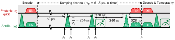
Figure S2: Experimental sequence for a damping channel simulation. Density matrices at the arrows are shown in detail in the text.

In our experiment, the damping channel is realized by using the control pulse sequence in Fig. 3(a) in the main text. To explain the protocol, we analyze the procedures in detail as follows.

1. The initial state of photonic qubit is $\rho_{\mathrm{in}}$, and the ancilla qubit is initialized to ground state $\rho_{\mathrm{a}}=\left|g\right\rangle\left\langle g\right|$. So, the input system of the system is

   $$\rho_{0}=\rho_{\mathrm{a}}\otimes\rho_{{\rm in}}=\left[\begin{array}[]{cc}1&0\\ 0&0\end{array}\right]\otimes\left[\begin{array}[]{cc}a&b\\ c&d\end{array}\right].$$ (S.87)

2. After applying $X_{\theta}$ ($U_{X}\left(\theta\right)=e^{-i\frac{\theta}{2}\mathbf{X}}$) to the ancilla qubit, we have

   $$\rho_{0}\mapsto\rho_{1} =U_{\mathbf{X}}\left(\theta\right)\rho_{0}U_{\mathbf{X}}^{\dagger}\left(\theta\right)$$ (S.88)

   $$=\left[\begin{array}[]{cc}\cos^{2}\left(\frac{\theta}{2}\right)&i\sin\left(\frac{\theta}{2}\right)\cos\left(\frac{\theta}{2}\right)\\ -i\sin\left(\frac{\theta}{2}\right)\cos\left(\frac{\theta}{2}\right)&\sin^{2}\left(\frac{\theta}{2}\right)\end{array}\right]\otimes\left[\begin{array}[]{cc}a&b\\ c&d\end{array}\right].$$ (S.93)

3. Due to the dispersive ancilla-photonic qubit interaction, a controlled-Z (CZ) gate can be obtained after a duration of $\pi/\chi_{{\rm{s}}}$, thus

   $$\rho_{1}\mapsto\rho_{2} =U_{\mathrm{CZ}}\rho_{1}U_{\mathrm{CZ}}^{\dagger}$$ (S.94)

   $$=\left[\begin{array}[]{cc}\cos^{2}\left(\frac{\theta}{2}\right)\left[\begin{array}[]{cc}a&b\\ c&d\end{array}\right]&i\sin\left(\frac{\theta}{2}\right)\cos\left(\frac{\theta}{2}\right)\left[\begin{array}[]{cc}a&-b\\ c&-d\end{array}\right]\\ -i\sin\left(\frac{\theta}{2}\right)\cos\left(\frac{\theta}{2}\right)\left[\begin{array}[]{cc}a&b\\ -c&-d\end{array}\right]&\sin^{2}\left(\frac{\theta}{2}\right)\left[\begin{array}[]{cc}a&-b\\ -c&d\end{array}\right]\end{array}\right].$$ (S.105)

4. After applying the second $X_{-\theta}$ (a unitary operation $U_{X}\left(-\theta\right)=e^{i\frac{\theta}{2}\mathbf{X}}$) to the ancilla qubit, we have

   $$\rho_{2}\mapsto\rho_{3} =U_{\mathbf{X}}\left(-\theta\right)\rho_{2}U_{\mathbf{X}}^{\dagger}\left(-\theta\right)$$ (S.106)

   $$=\left[\begin{array}[]{cc}\left[\begin{array}[]{cc}a&b{\rm cos}\left(\theta\right)\\ c{\rm cos}\left(\theta\right)&d{\rm cos}^{2}\left(\theta\right)\end{array}\right]&\left[\begin{array}[]{cc}0&-ib{\rm sin}\left(\theta\right)\\ 0&-id{\rm cos}\left(\theta\right){\rm sin}\left(\theta\right)\end{array}\right]\\ \left[\begin{array}[]{cc}0&0\\ ic{\rm sin}\left(\theta\right)&id{\rm cos}\left(\theta\right){\rm sin}\left(\theta\right)\end{array}\right]&\left[\begin{array}[]{cc}0&0\\ 0&d{\rm sin}^{2}\left(\theta\right)\end{array}\right]\end{array}\right].$$ (S.117)

5. After implementing a measurement-based adaptive operation on the photonic qubit, we have

   $$\rho_{3}\mapsto\rho_{4} =\left[\left|g\right\rangle\left\langle g\right|\otimes\mathbf{I}\right]\rho_{3}\left[\left|g\right\rangle\left\langle g\right|\otimes\mathbf{I}\right]^{\dagger}+\left[\left|e\right\rangle\left\langle e\right|\otimes\mathbf{X}\right]\rho_{3}\left[\left|e\right\rangle\left\langle e\right|\otimes\mathbf{X}\right]^{\dagger}$$ (S.118)

   $$=\left[\begin{array}[]{cc}a&b{\rm cos}\left(\theta\right)\\ c{\rm cos}\left(\theta\right)&d{\rm cos}^{2}\left(\theta\right)\end{array}\right]+\left[\begin{array}[]{cc}d{\rm sin}^{2}\left(\theta\right)&0\\ 0&0\end{array}\right]$$ (S.123)

   $$=\left[\begin{array}[]{cc}a+d{\rm sin}^{2}\left(\theta\right)&b{\rm cos}\left(\theta\right)\\ c{\rm cos}\left(\theta\right)&d{\rm cos}^{2}\left(\theta\right)\end{array}\right].$$ (S.126)

Comparing to the definition for a damping channel (Eq. S.21), we realize a damping channel to the photonic qubit with $\gamma=\sin^{2}\left(\theta\right)$.

Similar to the case of the dephasing channel, we have

$$\frac{1}{T_{1}^{c}} = -\frac{{\rm ln}({\rm cos}^{2}\theta)}{\tau_{0}}+\frac{1}{T_{1}^{0}},$$ (S.127)

$$\frac{1}{T_{2}^{c}} = -\frac{{\rm ln}({\rm cos}^{2}\theta)}{2\tau_{0}}+\frac{1}{T_{2}^{0}},$$ (S.128)

where $\tau_{0}$ is the time interval, and $T_{1}^{0}$, $T_{2}^{0}$ are the intrinsic decoherence times of the photonic qubit ($\theta=0^{\circ}$). In the main text, we get $T_{1}^{0}=137\pm 4~{}{\mathrm{\mu}}$s and $T_{2}^{0}=237\pm 3~{}{\mathrm{\mu}}$s, which agree well with $T_{1}^{{\rm{s}}}=143~{}{\mathrm{\mu}}$s and $T_{2}^{{\rm{s}}}=250~{}{\mathrm{\mu}}$s, respectively.

III.3 Arbitrary channel simulation

III.3.1 Simulation of arbitrary quantum channel

Following the proposal by Wang et al. Wang et al. (2013), we realize the arbitrary single-qubit channel by a convex combination of quasiextreme channels, where only a single ancilla qubit is required. As shown in Fig. 1(c) in the main text, the ancilla qubit is firstly prepared to a superposition state as

$$\rho_{\mathrm{a}}=X\left(\gamma_{p}\right)\left|g\right\rangle\left\langle g\right|X^{\dagger}\left(\gamma_{p}\right),$$ (S.129)

where $X\left(\theta\right)=e^{-i\frac{\theta}{2}\mathbf{X}}=\cos\frac{\theta}{2}\mathbf{I}-i\sin\frac{\theta}{2}\mathbf{X}$. Then, a projective measurement on the ancilla qubit in the computational basis is applied, and different channel branches are implemented according to the measurement result. This can be represented by the quantum instrument Wilde (2013)

$$\mathcal{E}:\,\rho\mapsto\mathcal{E}_{1}\otimes\left|g\right\rangle\left\langle g\right|+\mathcal{E}_{2}\otimes\left|e\right\rangle\left\langle e\right|.$$ (S.130)

Here, $\mathcal{E}_{j}$ with $j=0,1$ is the quasiextreme channel, which can be represented as

$$\mathcal{E}_{j}:\,\rho \mapsto U\left(\overrightarrow{\varphi}\right)\left[\left|g\right\rangle\left\langle g\right|\otimes I\right]X\left(2\gamma_{2}\right)U_{CZ}\left[X\left(2\gamma_{1}\right)\otimes U\left(\overrightarrow{\delta}\right)\right]\rho\left\{U\left(\overrightarrow{\varphi}\right)\left[\left|g\right\rangle\left\langle g\right|\otimes I\right]X\left(2\gamma_{2}\right)U_{CZ}\left[U\left(\overrightarrow{\delta}\right)\otimes X\left(2\gamma_{1}\right)\right]\right\}^{\dagger}$$ (S.131)

$$+U\left(\overrightarrow{\varphi}\right)\left[\left|e\right\rangle\left\langle e\right|\otimes X\right]X\left(2\gamma_{2}\right)U_{CZ}\left[X\left(2\gamma_{1}\right)\otimes U\left(\overrightarrow{\delta}\right)\right]\rho\left\{U\left(\overrightarrow{\varphi}\right)\left[\left|e\right\rangle\left\langle e\right|\otimes X\right]X\left(2\gamma_{2}\right)U_{CZ}\left[U\left(\overrightarrow{\delta}\right)\otimes X\left(2\gamma_{1}\right)\right]\right\}^{\dagger}$$

with parameters $\left\{\overrightarrow{\delta^{\left(j\right)}},\,\gamma_{1}^{\left(j\right)},\,\gamma_{2}^{\left(j\right)},\,\overrightarrow{\varphi^{\left(j\right)}}\right\}$, and unitary operation

$$U\left(\overrightarrow{\varphi}\right)=\left[\begin{array}[]{cc}\cos\frac{\varphi_{1}}{2}-i\sin\frac{\varphi_{1}}{2}\cos\frac{\varphi_{2}}{2}&-i\sin\frac{\varphi_{1}}{2}\sin\frac{\varphi_{2}}{2}e^{-i\varphi_{3}}\\ -i\sin\frac{\varphi_{1}}{2}\sin\frac{\varphi_{2}}{2}e^{i\varphi_{3}}&\cos\frac{\varphi_{1}}{2}+i\sin\frac{\varphi_{1}}{2}\cos\frac{\varphi_{2}}{2}\end{array}\right]$$ (S.132)

with $\varphi_{1,2,3}\in\left[0,2\pi\right]$. Therefore, there are 17 parameters in total, including $\gamma_{p}$ and two sets of $8$ parameters for quasiextreme channels. Actually, the dephasing and damping channels are two examples of quasiextreme channels. For a dephasing channel, we have $\gamma_{p}=0$ and $\left\{\overrightarrow{\delta^{\left(0\right)}},\,\gamma_{1}^{\left(0\right)},\,\gamma_{2}^{\left(0\right)},\,\overrightarrow{\varphi^{\left(0\right)}}\right\}=\left\{\left(0,0,0\right),0,\theta,\left(0,0,1\right)\right\}$. For a damping channel, we have $\gamma_{p}=0$ and $\left\{\overrightarrow{\delta^{\left(0\right)}},\,\gamma_{1}^{\left(0\right)},\,\gamma_{2}^{\left(0\right)},\,\overrightarrow{\varphi^{\left(0\right)}}\right\}=\left\{\left(0,0,0\right),\theta,-\theta,\left(0,0,1\right)\right\}$.

III.3.2 Random qubit channel

In our experiment, to demonstrate the ability of simulating arbitrary single-qubit channel, we first generate a single-qubit channel numerically with 12 random numbers in a target process matrix $\chi_{\mathrm{T}}$ that satisfy certain constraints Bhandari and Peters (2016). For the experimental results shown in the main text, we generated 6 random qubit channels as the targets for arbitrary quantum channel simulation. Here, we show the target $\chi_{\mathrm{T}}$ for channel arbi. 1 as an example

$$\chi_{\mathrm{T}}^{\left(1\right)}=\left(\begin{array}[]{cccc}0.362762&0.0143269\,+0.0767813i&-0.0305766+0.075406i&-0.00589476-0.134834i\\ 0.0143269\,-0.0767813i&0.22118&0.00589476\,+0.0979485i&-0.0331165-0.075406i\\ -0.0305766-0.075406i&0.00589476\,-0.0979485i&0.300734&0.0143269\,+0.027254i\\ -0.00589476+0.134834i&-0.0331165+0.075406i&0.0143269\,-0.027254i&0.115325\end{array}\right).$$ (S.133)

For a given target process matrix $\chi_{\mathrm{T}}$, the $17$ parameters for the arbitrary channel simulation are determined through numerical optimization that reduces the difference between $\chi_{\mathrm{sim}}$ and $\chi_{\mathrm{T}}$. Here, $\chi_{\mathrm{sim}}$ is the simulation result for the quantum circuit shown in Fig. 1(c) in the main text. Then, we implement the channel with the experimental sequence shown in Fig. 4(a) in the main text with the optimized $17$ parameters. The obtained experimental quantum channel $\chi_{\mathrm{E}}$ for the arbi. 1 is

$$\chi_{\mathrm{E}}^{\left(1\right)}=\left(\begin{array}[]{cccc}0.352118&0.0205553\,+0.0697286i&-0.0117642+0.0543421i&-0.00241937-0.107611i\\ 0.0205553\,-0.0697286i&0.244587&0.00241937\,+0.0722139i&-0.0386366-0.0543421i\\ -0.0117642-0.0543421i&0.00241937\,-0.0722139i&0.251896&0.0205553\,+0.0262903i\\ -0.00241937+0.107611i&-0.0386366+0.0543421i&0.0205553\,-0.0262903i&0.151398\end{array}\right).$$ (S.134)

III.3.3 Characterization of quantum channels

To characterize the performance of the experiment for arbitrary quantum channel simulation, we introduce two different figures of merit. The first one is the fidelity of state generation

$$F_{\mathrm{G}}=\mathrm{inf}_{\rho}\sqrt{\sqrt{\mathcal{E}_{\mathrm{T}}\left(\rho\right)}\left[\mathcal{E}_{\mathrm{E}}\left(\rho\right)\right]\sqrt{\mathcal{E}_{\mathrm{T}}\left(\rho\right)}}.$$ (S.135)

The physical meaning of $F_{\mathrm{G}}$ is the fidelity of the output quantum state $\mathcal{E}_{\mathrm{E}}\left(\rho\right)$ when we use the quantum channel to manipulate the quantum state for a given input compared with the result of the target quantum channel $\mathcal{E}_{\mathrm{T}}\left(\rho\right)$. Therefore, $F_{\mathrm{G}}$ is the worst fidelity of the quantum state generated by the experimental channel.

The other one is the measure of discriminating quantum channels. For two channels $\mathcal{E}_{1}$ and $\mathcal{E}_{2}$, the diamond distance is Wilde (2013)

$$D_{\diamond}=\left|\left|\mathcal{E}_{1}-\mathcal{E}_{2}\right|\right|_{\diamond}=\mathrm{sup}_{\rho}\left|\left|\left(\mathcal{E}_{1}\otimes\mathrm{Id}\right)\left(\rho\right)-\left(\mathcal{E}_{2}\otimes\mathrm{Id}\right)\left(\rho\right)\right|\right|_{1},$$ (S.136)

where the trace norm

$$\left|\left|T\right|\right|_{1}\equiv\mathrm{Tr}\sqrt{T^{\dagger}T}.$$ (S.137)

The diamond distance $D_{\diamond}\in\left[0,2\right]$ is related to the minimal probability $p_{\mathrm{dist}}=\frac{1}{2}-\frac{1}{4}D_{\diamond}$ of distinguishing two channels by allowing quantum entangled states between the channel and an ancillary space.

In the main text, both $F_{\mathrm{G}}$ and $D_{\diamond}$ are shown for different number of channel repetition $n$. It is shown that $F_{G}$ increases with $n$ while $D_{\diamond}$ decreases with $n$ for certain channels. To explain this behavior, we also present $D_{\diamond}$ between the target channel $\chi_{\mathrm{T}}$ (experimental channel $\chi_{\mathrm{E}}$) and the depolarization channel with $p=\frac{3}{4}$

$$\chi_{\mathrm{dpl}}=\frac{1}{4}\left[\begin{array}[]{cccc}1&0&0&0\\ 0&1&0&0\\ 0&0&1&0\\ 0&0&0&1\end{array}\right].$$ (S.138)

The results are presented in Fig. S3. These results indicate that repetitive arbitrary quantum channel eventually approaches a depolarization channel, therefore the distance between the target channel and the experimental channel may be closer after several rounds of repetition.

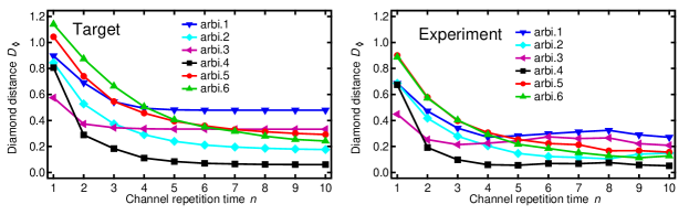
Figure S3: Diamond distances $D_{\diamond}$ between the target channel $\chi_{\mathrm{T}}$ (experimental channel $\chi_{\mathrm{E}}$) and the depolarization channel with $p=\frac{3}{4}$.

III.3.4 Correction of the measurement-induced phase shift

The measurement-induced phase on the photonic qubit does not commute with other processes in the arbitrary channel simulation. So we cannot ignore it during the experiment and deal with it in the final data analysis as for the cases of the dephasing and damping channel simulations. Instead, we experimentally eliminate this extra phase by modifying the measurement-adaptive sequence, as shown in Fig. S4.

In the arbitrary channel simulation [Fig. 4(a) of the main text], there are two measurement-adaptive processes: one is to get the quantum random number for deciding different branches and the other one is used in each branch. In our experiment, we want to keep the time interval between measurement and the following rotation pulse constant (320 ns) to minimize extra ancilla decoherence during this time interval. However, the measurement-adaptive sequence in Fig. S4(a) (used in both dephasing and damping channel simulations) will not lead to the same phase on the photonic qubit when associated with $\left|g\right\rangle$ and $\left|e\right\rangle$ respectively. To solve this problem, the measurement-adaptive sequence is replaced by Fig. S4(b). The time interval between the pre-rotation pulse on the ancilla and the measurement is increased such that the time interval between the pre-rotation and the $\pi$ pulse following the measurement is $(4\pi-0.3)/\chi_{{\rm{s}}}$. Here $0.3/\chi_{{\rm{s}}}$ corresponds to $17^{\circ}$ rotation of $\left|1\right\rangle$ state of the photonic qubit due to the cross Kerr between the readout cavity and the photonic qubit, independent of the ancilla state. If the measurement outcome of the ancilla state is $\left|e\right\rangle$, the $\pi$ pulse brings the ancilla to $\left|g\right\rangle$ after acquiring a total 4$\pi$ phase for $\left|e\right\rangle\left|1\right\rangle$ state (including the measurement-induced phase). Here, in the joint state notation the letters represent the ancilla states while the numbers correspond to the photonic qubit states. On the other hand, if the measurement outcome of the ancilla state is $\left|g\right\rangle$, the $\pi$ pulse after the measurement brings the ancilla to $\left|e\right\rangle$ to acquire an extra phase during the following $(2\pi-0.3)/\chi_{{\rm{s}}}$ interval before a second conditional $\pi$ pulse flips the ancilla back to $\left|g\right\rangle$. In the end, the original $\left|g\right\rangle\left|1\right\rangle$ also acquires a 2$\pi$ phase.

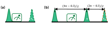
Figure S4: Correction of the measurement-induced phase shift in the arbitrary channel simulation. The measurement-adaptive sequence (a) used in both dephasing and damping channel simulations is replaced by the new one in (b). The goal is to acquire integer multiples of 2$\pi$ phase for both $\left|g\right\rangle\left|1\right\rangle$ and $\left|e\right\rangle\left|1\right\rangle$. Here $0.3/\chi_{{\rm{s}}}$ is the time interval for $\left|e\right\rangle\left|1\right\rangle$ state under free evolution to acquire a phase of $17^{\circ}$, which is the measurement-induced phase on both $\left|g\right\rangle\left|1\right\rangle$ and $\left|e\right\rangle\left|1\right\rangle$.

IV Discussions

IV.1 The limitations of dephasing and damping rates

The ancilla qubit facilitates all channel simulations. Consequently, its intrinsic decoherence prevents an arbitrary fast dephasing or damping rate, and eventually sets a limit on these rates. In this part, we show how the ancilla decoherence affects the simulated dephasing and damping rates in the corresponding channels.

IV.1.1 The dephasing channel

First, we show that the dephasing of the ancilla will not affect the dephasing channel. The dephasing channel relies on the dispersive interaction between the ancilla and the photonic qubit. Explicitly, the joint state $\left|e\right\rangle\left|1\right\rangle$ acquires a phase relative to other three states $\left|e\right\rangle\left|0\right\rangle$, $\left|g\right\rangle\left|1\right\rangle$, and $\left|g\right\rangle\left|0\right\rangle$ with a rate equal to the dispersive interaction strength $\chi_{{\rm{s}}}$. Before the projective measurement in the channel simulation, the dephasing of the ancilla only changes the sign associated with $\left|e\right\rangle$ state, which has no observable effect on the following projective measurement and adaptive control. Therefore, the dephasing channel remains unaffected, and we only need to consider thermal excitation and ancilla decay.

After a waiting time of $60~{}{\mathrm{\mu}}$s, the ancilla qubit can be considered in a thermal equilibrium state with an $\left|e\right\rangle$ state population $n_{{\rm{th}}}=0.87\%$ based on an independent calibration experiment. For an initial $\left|e\right\rangle$ state, the following channel simulation still works well except that the probability causing a phase flip of the photonic qubit changes from ${\rm sin}^{2}(\theta/2)$ to ${\rm cos}^{2}(\theta/2)$ due to the exchange of $\left|g\right\rangle$ and $\left|e\right\rangle$.

Between the $X_{\theta}$ gate and the adaptive $\pi$ pulse, random decay of the ancilla qubit from $\left|e\right\rangle$ to $\left|g\right\rangle$ causes random phase on $\left|1\right\rangle$ state instead of a complete phase flip. Therefore, this will reduce the phase-flip probability of $\left|1\right\rangle$. On average, we can treat this reduction factor as $1-p_{1}/2$ with $p_{1}=(3\pi/\chi_{{\rm{s}}})/T_{1}$, the probability of having an ancilla decay. The ancilla upwards transition probability from $\left|g\right\rangle$ to $\left|e\right\rangle$ is tiny during the short channel simulation process and can be neglected. Combining the above two effects, thermal excitation during $\tau_{0}$ and ancilla decay, we get the final phase flip probability for the photonic qubit as a function of the rotation angle in $X_{\theta}$:

$$p_{\phi}^{{\rm{lim}}}=(1-n_{{\rm{th}}}){\rm sin}^{2}(\theta/2)(1-p_{1}/2)+n_{{\rm{th}}}{\rm cos}^{2}(\theta/2)(1-p_{1}/2).$$ (S.139)

Then we can get the upper limit of the external and controllable dephasing rate in our channel simulation:

$$\Gamma_{\phi}^{{\rm lim}}=-\frac{{\rm ln}(1-2p_{\phi}^{{\rm{lim}}})}{\tau_{0}},$$ (S.140)

which is used for Fig. 2(e) in the main text.

IV.1.2 The damping channel

The ancilla dephasing will not affect the performance of the damping channel, provided the initial state of the photonic qubit is at $\left|1\right\rangle$ state. This is because the ancilla dephasing during the the parity-type protocol ($X_{\theta}$, $\pi/\chi_{{\rm{s}}}$, $X_{-\theta}$) only flips the phase on $\left|e\right\rangle\left|1\right\rangle$, and this flip has no effect on the following projective measurement and adaptive control. However, if the initial state is a superposition of $\alpha\left|0\right\rangle+\beta\left|1\right\rangle$, the ancilla dephasing will affect the resulting channel. Here, we focus on the case of an initial $\left|1\right\rangle$ state of the photonic qubit, since this is a direct reflection of the damping rate of this channel [Fig. 3(b) of the main text]. Therefore, we only need to consider the thermal excitation and energy decay of the ancilla.

Similar to the case of the damping channel, after a waiting time of $60~{}{\mathrm{\mu}}$s, the ancilla qubit can be treated in a thermal equilibrium state. For an initial $\left|e\right\rangle$ state of the ancilla, the following channel simulation also works well except that the probability causing the photonic qubit decay changes from ${\rm sin}^{2}\theta$ to ${\rm cos}^{2}\theta$ due to the exchange of $\left|g\right\rangle$ and $\left|e\right\rangle$.

During the parity-type protocol, random decay of the ancilla qubit from $\left|e\right\rangle$ to $\left|g\right\rangle$ [with a probability of $p_{1}=(\pi/\chi_{{\rm{s}}})/T_{1}$] changes the photonic qubit damping probability to ${\rm sin}^{2}(\theta/2)$ since only the second $X_{-\theta}$ is effective on the ancilla. The ancilla decay process could also happen with a probability $p_{2}$ during the measurement and the following waiting time. Then the adaptive $\pi$ rotation will flip the ancilla to $\left|e\right\rangle$ and mess up with the final GRAPE pulse to flip the photonic qubit from $\left|1\right\rangle$ to $\left|0\right\rangle$. Since the photonic qubit state is unknown and we simply treat this process causes a damping with a probability of 1/2 (completely mixed photonic qubit state). These processes will reduce the probability of damping the photonic qubit, and based on a probability calculation we finally get the damping probability limit $\gamma^{{\rm{lim}}}$ the channel:

$$\gamma^{{\rm{lim}}} =(1-n_{{\rm{th}}})\{[1-p_{1}{\rm sin}^{2}(\theta/2)](1-p_{2}){\rm sin}^{2}\theta+[1-p_{1}{\rm sin}^{2}(\theta/2)]p_{2}/2+p_{1}{\rm sin}^{2}(\theta/2){\rm sin}^{2}(\theta/2)\}$$ (S.141)

$$+n_{{\rm{th}}}\{[1-p_{1}{\rm cos}^{2}(\theta/2)](1-p_{2}){\rm cos}^{2}\theta+[1-p_{1}{\rm cos}^{2}(\theta/2)]p_{2}/2+p_{1}{\rm cos}^{2}(\theta/2){\rm sin}^{2}(\theta/2)\}$$ (S.142)

Then we can get the upper limit of the external and controllable damping rate in our channel simulation:

$$\Gamma_{1}^{{\rm lim}}=-\frac{{\rm ln}(1-\gamma^{{\rm{lim}}})}{\tau_{0}},$$ (S.143)

which is used for Fig. 3(e) in the main text.

IV.2 Fit of process fidelity curves in the dephasing and damping channel simulations

The channel simulation results presented in the main text are obtained with a waiting time $60~{}{\mathrm{\mu}}$s ($\tau_{0}\approx 61~{}{\mathrm{\mu}}$s). To see the channel behavior in a short time scale, we also perform simulations with a waiting time $5~{}{\mathrm{\mu}}$s [Figs. S5(c) and (g)]. The channel process fidelity, defined as the overlap of the measured $\chi$ matrix and $\chi_{{\rm{I}}}$ for the identity operation, decays exponentially when $\theta$ is small, but deviates from the exponential behavior when $\theta$ is large. In addition, we perform the experiment with $\theta>90^{\circ}$ as well, which corresponds to a phase-flip probability $p_{\phi}>1/2$ for the dephasing channel [Fig. S5(d)] or $-1\leq\sqrt{1-\gamma}\leq 0$ for the damping channel [Fig. S5(h)]. In these two cases, the process fidelity oscillates after each extra channel repetition.

In order to understand the decay and oscillation, and to verify the channel performance, we can do full numerical simulations and compare the results with the experimental data. To save time, we only numerically simulate the $\chi$ matrices of two processes with QuTip in Python Johansson et al. (2012, 2013): free evolution of the system for $60~{}{\mathrm{\mu}}$s and $5~{}{\mathrm{\mu}}$s respectively; and treat the channels as ideal ones because of the large number of different channels. Then, for different input states we can simply interleave the corresponding free evolution process and the ideal channel (dephasing or damping) for $n$ times to get the final states, and in turn the total process fidelity $\chi_{\theta}(t)$ at different times. We finally fit the experimental data with $F_{\chi}(t)=A[Tr(\chi_{{\rm I}}\chi_{\theta}(t)-0.25]+0.25$, where $A$ is a pre-factor to take into account the reduction due to the encoding and decoding processes in the experiment but not in the simulation, and 0.25 is final saturation value in the long time limit. The fitted results are shown in Fig. S5 connected with dashed lines to guide the eye, in excellent agreement with the experiment. The extracted $\theta$’s are plotted in Fig. S6, which also agree well with the externally controlled rotation angle in the experiment.

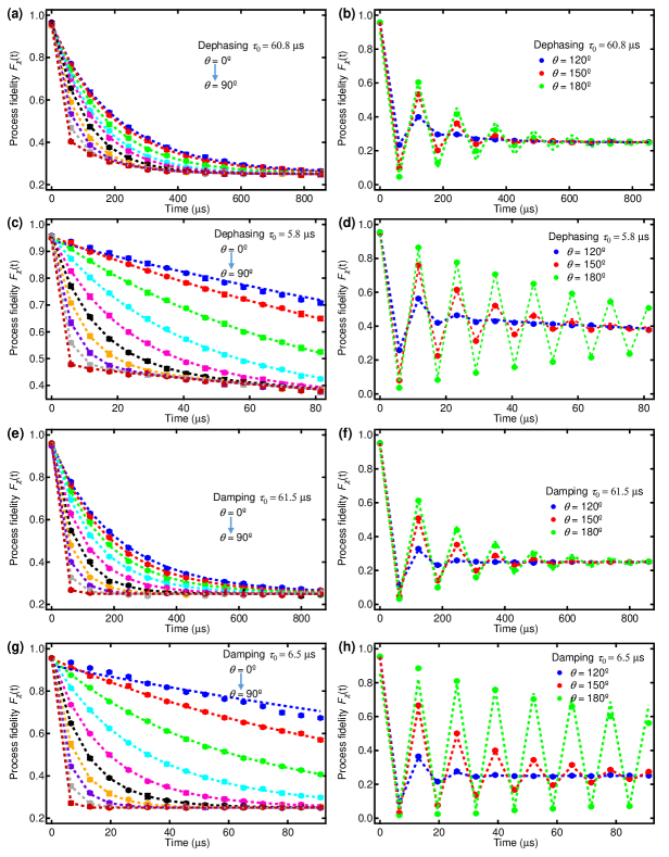
Figure S5: Fit process fidelity curves with simulated $\chi$ matrices. We do numerical simulations with QuTip to compare with the experimental data. To save time, we only numerically simulate the $\chi$ matrices of two processes: free evolution of the system for $60~{}{\mathrm{\mu}}$s and $5~{}{\mathrm{\mu}}$s respectively; and treat the channels as ideal ones because of the large number of different channels. Due to the repetitive nature of the channel, we then simply interleave the corresponding free evolution process and the ideal channel (dephasing or damping) for $n$ times to get the total process matrix $\chi(\theta)$ at different times. Finally, the experimental data are fitted with $F_{\chi}=A[Tr(\chi_{{\rm I}}\chi(\theta)-0.25]+0.25$, where $\chi_{{\rm I}}$ is for an identity channel, $A$ is a pre-factor to take into account the reduction due to the encoding and decoding processes in the experiment but not in the simulation, and 0.25 is final saturation value in the long time limit. The fitted results are connected with dashed lines to guide the eye and are in excellent agreement with the experiment.

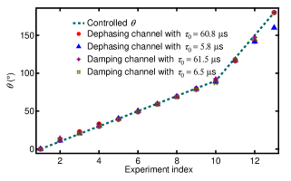
Figure S6: $\theta$ extracted from fit of the process fidelity curves in Fig. S5. Points are the extracted $\theta$ (12 of them), in good agreement with the externally controlled rotation angles in the experiment (connected with a dashed line).

References

- Reagor et al. (2013) M. Reagor, H. Paik, G. Catelani, L. Sun, C. Axline, E. Holland, I. M. Pop, N. A. Masluk, T. Brecht, L. Frunzio, M. H. Devoret, L. I. Glazman, and R. J. Schoelkopf, “Ten milliseconds for aluminum cavities in the quantum regime,” Appl. Phys. Lett. 102, 192604 (2013).
- Reagor et al. (2016) M. Reagor, W. Pfaff, C. Axline, R. W. Heeres, N. Ofek, K. Sliwa, E. Holland, C. Wang, J. Blumoff, K. Chou, M. J. Hatridge, L. Frunzio, M. H. Devoret, L. Jiang, and R. J. Schoelkopf, “Quantum memory with millisecond coherence in circuit qed,” Phys. Rev. B 94, 014506 (2016).
- Hatridge et al. (2011) M. Hatridge, R. Vijay, D. H. Slichter, J. Clarke, and I. Siddiqi, “Dispersive magnetometry with a quantum limited SQUID parametric amplifier,” Phys. Rev. B 83, 134501 (2011).
- Roy et al. (2015) T. Roy, S. Kundu, M. Chand, A. M. Vadiraj, A. Ranadive, N. Nehra, M. P. Patankar, J. Aumentado, A. A. Clerk, and R. Vijay, “Broadband parametric amplification with impedance engineering: Beyond the gain-bandwidth product,” Appl. Phys. Lett. 107, 262601 (2015).
- Kamal et al. (2009) A. Kamal, A. Marblestone, and M. H. Devoret, “Signal-to-pump back action and self-oscillation in double-pump Josephson parametric amplifier,” Phys. Rev. B 79, 184301 (2009).
- Murch et al. (2013) K. W. Murch, S. J. Weber, C. Macklin, and I. Siddiqi, “Observing single quantum trajectories of a superconducting quantum bit,” Nature 502, 211 (2013).
- Hu et al. (2018) L. Hu, Y. Ma, W. Cai, X. Mu, Y. Xu, W. Wang, Y. Wu, H. Wang, Y. Song, C. Zou, S. M. Girvin, L.-M. Duan, and L. Sun, “Demonstration of quantum error correction and universal gate set on a binomial bosonic logical qubit,” arXiv:1805.09072 (2018).
- Nielsen and Chuang (2000) M. A. Nielsen and I. L. Chuang, Quantum Computation and Quantum Information (Cambridge Univ. Press, 2000).
- Bhandari and Peters (2016) R. Bhandari and N. A. Peters, “On the general constraints in single qubit quantum process tomography,” Sci. Rep. 6, 26004 (2016).
- Carmichael (2003) H. J. Carmichael, “Statistical methods in quantum optics 1: Master equations and fokker-planck equations (theoretical and mathematical physics),” (2003).
- Petruccione and Breuer (2002) F. Petruccione and H. Breuer, The theory of open quantum systems (Oxford University Press, 2002) p. 625.
- Gardiner et al. (2004) C. Gardiner, P. Zoller, and P. Zoller, Quantum noise: a handbook of Markovian and non-Markovian quantum stochastic methods with applications to quantum optics, Vol. 56 (Springer Science & Business Media, 2004).
- Krastanov et al. (2015) S. Krastanov, V. V. Albert, C. Shen, C.-L. Zou, R. W. Heeres, B. Vlastakis, R. J. Schoelkopf, and L. Jiang, “Universal control of an oscillator with dispersive coupling to a qubit,” Phys. Rev. A 92, 040303 (2015).
- Kliesch et al. (2011) M. Kliesch, T. Barthel, C. Gogolin, M. Kastoryano, and J. Eisert, “Dissipative Quantum Church-Turing Theorem,” Phys. Rev. Lett. 107, 120501 (2011).
- Sweke et al. (2014) R. Sweke, I. Sinayskiy, and F. Petruccione, “Simulation of single-qubit open quantum systems,” Phys. Rev. A 90, 022331 (2014).
- Wang et al. (2013) D. S. Wang, D. W. Berry, M. C. De Oliveira, and B. C. Sanders, “Solovay-kitaev decomposition strategy for single-qubit channels,” Phys. Rev. Lett. 111, 130504 (2013).
- Wilde (2013) M. M. Wilde, Quantum Information Theory (Cambridge University Press, 2013).
- Johansson et al. (2012) J. R. Johansson, P. D. Nation, and F. Nori, “Qutip: An open-source python framework for the dynamics of open quantum systems,” Comp. Phys. Comm. 183, 1760 (2012).
- Johansson et al. (2013) J. R. Johansson, P. D. Nation, and F. Nori, “Qutip 2: A python framework for the dynamics of open quantum systems,” Comp. Phys. Comm. 184, 1234 (2013).