Dynamical Evolution of the Early Solar System

Abstract

Several properties of the Solar System, including the wide radial spacing of the giant planets, can be explained if planets radially migrated by exchanging orbital energy and momentum with outer disk planetesimals. Neptune’s planetesimal-driven migration, in particular, has a strong advocate in the dynamical structure of the Kuiper belt. A dynamical instability is thought to have occurred during the early stages with Jupiter having close encounters with a Neptune-class planet. As a result of the encounters, Jupiter acquired its current orbital eccentricity and jumped inward by a fraction of an au, as required for the survival of the terrestrial planets and from asteroid belt constraints. Planetary encounters also contributed to capture of Jupiter Trojans and irregular satellites of the giant planets. Here we discuss the dynamical evolution of the early Solar System with an eye to determining how models of planetary migration/instability can be constrained from its present architecture.

1 INTRODUCTION

The first Solar System solids condensed 4.568 Gyr ago (see Kleine et al. 2009 for a review). This is considered as time zero in the Solar System history ($t_{0}$). Jupiter and Saturn have massive gas envelopes and must have formed within the lifetime of the protoplanetary gas disk. From observations we know that the protoplanetary gas disks last 2-10 Myr (e.g., Williams & Cieza 2011). Assuming that the Solar System is typical, Jupiter and Saturn should thus have formed within 2-10 Myr after $t_{0}$ (Kruijer et al. 2017). Geochemical constraints and numerical modeling suggest that the terrestrial planet formation ended much later, probably some 30-100 Myr after the gas disk dispersal (e.g., Jacobson et al. 2014).

The subject of this review is the dynamical evolution of planets and small bodies in the Solar System after the dispersal of the protoplanetary gas nebula. Here we are therefore not primarily concerned with the growth and gas-driven migration of planets (for that, see reviews of Kley & Nelson 2012 and Youdin & Kenyon 2013). The earliest epochs are obviously relevant, because they define the initial conditions from which the Solar System evolved. Ideally, this link should be emphasized, but physics of the protoplanetary disk stage is not understood well enough to make definitive predictions (except those discussed in Section 3). Instead, a common approach to studying the early dynamical evolution of the Solar System is that of reverse engineering, where the initial state and subsequent evolution are deduced from various characteristics of the present-day Solar System.

2 PLANETESIMAL-DRIVEN MIGRATION

Planetary formation is not an ideally efficient process. The growth of planets from smaller disk constituents can be frustrated, for example, when the orbits become dynamically excited. The accretion of bodies in the asteroid belt region (2-4 au) is thought to have ended when Jupiter formed and migrated in the gas disk (Walsh et al. 2011). The growth of bodies in the region of the Kuiper belt ($>$30 au), on the other hand, progressed at a leisurely pace, because the accretion clock was ticking slowly at large orbital periods, and probably terminated, for the most part, when the nebular gas was removed. As a result, in addition to planets, the populations of small bodies –commonly known as planetesimals– emerged in the early Solar System.

The gravitational interaction between planets and planetesimals has important consequences. For example, the gravitational torques of planets on planetesimals can generate the apsidal density waves in planetesimal disks (e.g., Ward & Hahn 1998). A modest degree of orbital excitation arising in a planetesimal disk at orbital resonances and/or from gravitational scattering between planetesimals can shut down the wave propagation. In this situation, the main coupling between planets and planetesimals arises during their close encounters when they exchange orbital momentum and energy.

Consider a mass $m$ of planetesimals ejected from the Solar System by a planet of mass $M$ and orbital radius $r$. From the conservation of the angular momentum it follows that the planet suffers a decrease $\delta r$ of orbital radius given by $\delta r/r\simeq-Cm/M$, where $C$ is a coefficient of the order of unity (Malhotra 1993). For example, if Jupiter at $r\simeq 5$ au ejects 15 $M_{\oplus}$ of planetesimals, where $M_{\oplus}$ is the Earth mass, it should migrate inward by $\delta r\simeq-0.2$ au. Conversely, outer planetesimals scattered by a planet into the inner Solar System would increase the planet’s orbital radius.

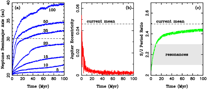
Figure 1: Planetesimal-driven migration in the outer Solar System. The outer planets were placed into a compact configuration with the semimajor axes $a_{5}=5.4$ au, $a_{6}=8.7$ au, $a_{7}=15.0$ au and $a_{8}=20.0$ au (index denotes planets in order of the heliocentric distance). The outer planetesimal disk at 20-30 au was resolved by 10,000 bodies and was given different masses in different $N$-body integrations (labeled in Earth masses, $M_{\oplus}$, in panel a). Panel (a): Outward migration of Neptune in different cases. The dashed line indicates the current mean semimajor axis of Neptune ($e_{8}=30.1$ au). Panel (b): Jupiter’s eccentricity becomes quickly damped by dynamical friction with scattered planetesimals. Panel (c): The evolution of Saturn/Jupiter period ratio, $P_{6}/P_{5}$, for $M_{\rm disk}=35$ $M_{\oplus}$. Secular resonances with the terrestrial planets and asteroids occur in the gray region ($2.1<P_{6}/P_{5}<2.3$).

Numerical simulations of planetesimal scattering in the outer Solar System show that Neptune, Uranus and Saturn tend to preferentially scatter planetesimals inward and therefore radially move outward. Jupiter, on the other hand, ejects planetesimals to Solar System escape orbits and migrates inward (Fernández & Ip 1984). This process is known as the planetesimal-driven migration. A direct evidence for the planetesimal-driven migration of Neptune is found in the Kuiper belt, where there are large populations of bodies in orbital resonances with Neptune (e.g., Pluto and Plutinos in the 3:2 resonance with Neptune; Malhotra 1993, 1995; Section 11).

The timescale and radial range of the planetesimal-driven migration depends on the total mass and distribution of planetesimals (Hahn & Malhotra 1999). Two migration regimes can be identified (Gomes et al. 2004). If the radial density of planetesimals exceeds certain value, the migration is self-sustained and Neptune proceeds to migrate outward (upper curves in Figure 1a). If, on the other hand, the radial mass density of planetesimals is low, the planet runs out of fuel and stops (the so-called damped migration; Gomes et al. 2004). The critical density is determined by the dynamical lifetime of planetesimals on planet-crossing orbits.

The critical mass density is near 1-1.5 $M_{\oplus}$ au^-1 but depends on other parameters as well. For example, a 20 $M_{\oplus}$ planetesimal disk extending from 20 au to 30 au with a surface density $\Sigma\propto 1/r$ is clearly super-critical (radial mass density 2 $M_{\oplus}$ au^-1). Neptune’s migration is self-sustained in this case and Neptune ends up migrating to the outer edge of the disk at 30 au. If the disk mass is higher than that, Neptune can even move beyond the original edge of the disk. A 5 $M_{\oplus}$ planetesimal disk with the same parameters, on the other hand, is sub-critical (mass density 0.5 $M_{\oplus}$ au^-1) and Neptune’s migration stalls just beyond 20 au (Figure 1). The planetesimal disk survives in the latter case, which may be relevant for the long-lived debris disks observed around other stars (Wyatt 2008).

For super-critical disks, the speed of planetary migration increases with planetesimal mass density. The Kuiper belt constrains require that the characteristic $e$-folding timescale of Neptune’s migration, $\tau$, satisfied $\tau\geq 10$ Myr (Section 11). This implies that the planetesimal disk at 20-30 au had mass $M_{\rm disk}\leq 20$ $M_{\oplus}$. For Neptune to migrate all the way to 30 au, as discussed above, $M_{\rm disk}\geq 15$ $M_{\oplus}$. Together, this implies $M_{\rm disk}\simeq 15$-20 $M_{\oplus}$ for the planetesimal disk between 20-30 au. Beyond 30 au, the planetesimal disk must have become sub-critical. The disk may have been truncated, for example, by photoevaporation (e.g., Adams 2010; see Section 11).

3 PLANETARY INSTABILITY

Planets form on nearly circular and coplanar orbits. The planetary orbits remain nearly circular and coplanar during planetesimal-driven migration, because the collective effect of small disk planetesimals on planets is to damp any excess motion due to eccentricity or inclination. This so-called dynamical ‘friction’ drives planetary orbits toward $e=0$ and $i=0$ ($e_{5}=0.002$ and $e_{6}=0.005$ at the end of the simulation with $M_{\rm disk}=35$ $M_{\oplus}$; Figure 1b). In contrast, Jupiter and Saturn have current mean eccentricities $e_{5}=0.046$ and $e_{6}=0.054$, respectively. Also, the orbits of Saturn and Uranus are significantly inclined ($i_{6}=0.90^{\circ}$ and $i_{7}=1.0^{\circ}$). This shows need for some excitation mechanism.

Tsiganis et al. (2005; also see Thommes et al. 1999) proposed that the excitation of planetary orbits occurred when Jupiter and Saturn crossed the 2:1 resonance during the planetesimal-driven migration. Because the planetary orbits diverge from each other (Jupiter moves in and Saturn out), the resonance is approached from a direction from which capture cannot occur. Instead, the orbits cross the 2:1 resonance and acquire modest eccentricities. This, in itself, would not be enough to provide the needed excitation (e.g., the orbits of Uranus and Neptune remained unaffected). The 2:1 resonant crossing, however, can trigger a dynamical instability in the outer Solar System with Uranus and/or Neptune eventually evolving onto Saturn-crossing orbits. A dynamical excitation of orbits then presumably happened during scattering encounters between planets. As a result of planetary encounters, Uranus and Neptune were thrown out into the outer planetesimal disk, where they stabilized and migrated to their current orbits (Figure 2).

This instability model, known as the ‘original’ Nice model (after a city in southern France where the model was conceived), has been successful in reproducing the orbits of the outer Solar System planets. It has also provided a scientific justification for the possibility that the Late Heavy Bombardment of the Moon was a spike in the impact record (Gomes et al. 2005, Levison et al. 2011; Section 13), and offered a convenient framework for understanding various other properties of the Solar System (e.g., Morbidelli et al. 2005, Nesvorný et al. 2007, Levison et al. 2008; Sections 6-12).

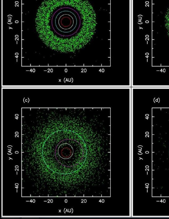
Figure 2: The original Nice model simulation showing the outer planets and planetesimals: (a) initial configuration; (b) early configuration, before Jupiter and Saturn reach the 2:1 resonance; (c) scattering of planetesimals after the orbital shift of Neptune (dark blue) and Uranus (light blue); (d) after ejection of planetesimals by planets.

The evolution of planets during the dynamical instability is stochastic. This means that small changes of the initial conditions can lead to different results. It is therefore insufficient to perform one or a few dynamical simulations. Instead, a statistical model must be developed, where many realizations of the same initial conditions are tested.

The initial conditions of a model can be informed from the gas-driven migration of planets during the protoplanetary disk phase. Hydrodynamic studies show that Jupiter and Saturn underwent a convergent migration in the gas disk with their orbits approaching each other. The orbits were subsequently captured into an orbital resonance. Under standard conditions (the gas surface density $\Sigma\simeq 1700$ g cm^-2 at 1 au from the Minimum Mass Solar Nebula model, MMSN, Weidenschilling 1977, Hayashi 1981; $\alpha$ viscosity $\simeq 10^{-3}$-$10^{-2}$, Shakura & Sunyaev 1973; aspect ratio $H/r\simeq 0.05$), the orbits cross the 2:1 resonance without being captured, because the convergent migration is too fast for capture to happen. They are eventually trapped in the 3:2 resonance (Masset & Snellgrove 2001, Morbidelli & Crida 2007, Pierens & Nelson 2008).

The 3:2 resonance configuration of the Jupiter-Saturn pair is the essential ingredient of the Grand Tack (GT) model (Walsh et al. 2011). In the GT model, Jupiter migrated down to $r\simeq 1.5$ au when the 3:2 resonance was established. After that, Jupiter and Saturn opened a common gap in the disk, the migration torques reversed their usual direction, and Jupiter, after executing the sailing maneuver of tacking, moved outward to beyond 5 au. The GT model helps to explain the small mass of Mars and asteroid belt, and mixing of the taxonomic types in the asteroid belt (Gradie & Tedesco 1982). Subsequent studies showed that capture of Jupiter and Saturn in the 2:1 resonance would be possible if planets migrated slowly in a low-mass and low-viscosity disk (Pierens et al. 2014). It is harder in this case, however, to obtain the torque reversal and stable outward migration.

Given these results, it is reasonable to expect that Jupiter and Saturn emerged from the protoplanetary disk with orbits locked in the 3:2 resonance (or, somewhat less likely, in the 2:1 resonance). The initial orbits of Uranus and Neptune should have been resonant as well (Morbidelli et al. 2007). In a MMSN disk with modest viscosity, capture of ice giants in the 3:2, 4:3 and 5:4 resonances is preferred. In a low-mass disk, instead, the 2:1 and 3:2 resonances are preferred. The latter case may apply if Uranus/Neptune formed late, near the end of the protoplanetary disk phase, as indicated by their low-mass gas envelopes.

The initial orbits of the outer planets in a fully resonant chain have not been considered in the original Nice model. Morbidelli et al. (2007) performed several simulations starting from the initially resonant conditions. They showed that the subsequent dynamical evolution of planets is qualitatively similar to that reported in Tsiganis et al. (2005). Still, none of these instability/migration models properly accounted for many Solar System constraints, including the secular architecture of the outer planet system, survival of the terrestrial planets, and orbital structure of the asteroid belt.

4 JUMPING JUPITER

In the original Nice model, Jupiter does not participate in the dynamical instability (i.e., there are no encounters of Jupiter with other planets). This is desirable because if Saturn had close encounters with Jupiter, the mutual scattering between Jupiter and Saturn would lead to a very strong orbital excitation, which has to be avoided. The strong dynamical instabilities between massive planets are thought to be responsible for the broad eccentricity distribution of the Jupiter-class exoplanets (Rasio & Ford 1996).

In Tsiganis et al. (2005), the orbital eccentricity of Jupiter, $e_{5}$, is generated when Jupiter and Saturn cross the 2:1 resonance during their planetesimal-driven migration. Additional changes of $e_{5}$ occur during encounters between Saturn and Uranus/Neptune, because the evolution of eccentricities is coupled via the Laplace-Lagrange equations (Murray & Dermott 1999). The Laplace-Lagrange equations applied to Jupiter and Saturn yield

$$e_{5}\exp\iota\varpi_{5} = e_{55}\exp\iota(g_{5}t+\phi_{5})+e_{56}\exp\iota(g_{6}t+\phi_{6})$$

$$e_{6}\exp\iota\varpi_{6} = e_{65}\exp\iota(g_{5}t+\phi_{5})+e_{66}\exp\iota(g_{6}t+\phi_{6})\ ,$$ (1)

where $e_{ij}$, $g_{i}$ and $\phi_{i}$ are amplitudes, frequencies and phases. Specifically, $g_{5}=4.24$ arcsec yr^-1, $g_{6}=28.22$ arcsec yr^-1, $e_{55}=0.044$, $e_{56}=-0.015$, $e_{66}=0.033$ and $e_{65}=0.048$ in the present Solar System.

Since $e_{55}>|e_{56}|$, Jupiter’s proper eccentricity mode is excited more that the forced mode. Conversely, during the 2:1 resonance crossing and Saturn’s encounters, the proper mode would end up being less excited than the forced one, leaving $e_{55}<|e_{56}|$ (Ćuk 2007). Therefore, while the excitation of Jupiter’s eccentricity is adequate in the original Nice model, the partition of $e_{5}$ in the modal amplitudes $e_{55}$ and $e_{56}$ is not. The most straightforward way to excite $e_{55}$ is to postulate that Jupiter have participated in planetary encounters with an ice giant, for example, with Uranus (Morbidelli et al. 2009a).

The slow migration of Jupiter and Saturn past the 2:1 resonance, which is a defining feature of the original Nice model (Figure 1c), is difficult to reconcile with several Solar System constrains, including the low Angular Momentum Deficit (AMD) of the terrestrial planets and the orbital structure of the asteroid belt (Sections 7 and 8). These constraints imply that the orbital period ratio of Jupiter and Saturn, $P_{6}/P_{5}$, must have discontinuously changed from $<$2.1 to at least $>$2.3 (Brasser et al. 2009, Morbidelli et al. 2010), perhaps because Jupiter and Saturn had encounters with an ice giant and their semimajor axes changed by a fraction of an au. The terrestrial planet constraint could be bypassed if the migration/instability of the outer planets happened early (Section 13), when the terrestrial planet formation was not completed, but the asteroid constraint applies independently of that.

These are the basic reasons behind the jumping-Jupiter model. Jupiter’s jump can be accomplished if Jupiter had close encounters with an ice giant with the mass similar to Uranus or Neptune. The scattering encounters with an ice giant would also help to excite the $e_{55}$ mode in Jupiter’s orbit, as needed to explain its present value. In addition, Jupiter’s planetary encounters provide the right framework for capture of Jupiter Trojans (Section 9) and irregular satellites (Section 10). The jumping-Jupiter model is therefore a compelling paradigm for the early evolution of the Solar System.

If Jupiter and Saturn started in the 3:2 resonance, where $P_{6}/P_{5}\simeq 1.5$, the easiest way to satisfy constraints is to have a few large jumps during planetary encounters such that $P_{6}/P_{5}$ changed from $\simeq$1.5 directly to $>$2.3. Dynamical models, in which the planetesimal-driven migration extracts Jupiter and Saturn from the 3:2 resonance and moves $P_{6}/P_{5}$ closer to 2 before the instability happens, are statistically unlikely (because there is a tendency for the instability to develop early, or not at all). If Jupiter and Saturn started in the 2:1 resonance instead, where $P_{6}/P_{5}\simeq 2$, the required jump is smaller and can be easier to accomplish in a numerical model (Pierens et al. 2014). This is the main advantage of the 2:1 resonance configuration over the 3:2 resonance configuration. All other considerations favor 3:2.

5 FIVE PLANET MODEL

The results of dynamical simulations, when contrasted with the observed properties of the present-day Solar System, can be used to backtrack the initial conditions from which the Solar System evolved. In one of the most complete numerical surveys conducted so far, Nesvorný & Morbidelli (2012; hereafter NM12) performed nearly $10^{4}$ simulations of the planetary migration/instability starting from hundreds of different initial conditions. A special attention was given to the cases with Jupiter and Saturn initially in the 3:2 and 2:1 orbital resonances. They experimented with different radial profiles and orbital distributions of disk planetesimals, different disk masses, etc.

The cases with four, five and six outer planets were tested, where the additional planets were placed onto resonant orbits between Saturn and Uranus, or beyond the initial orbit of Neptune. The cases with additional planets were considered in NM12, because it was found that they produce much better results than the four-planet case (see below). The masses of additional planets were set between 0.3 $M_{7}$ and 3 $M_{8}$, where $M_{7}=14.5$ $M_{\oplus}$ and $M_{8}=17.2$ $M_{\oplus}$ are the masses of Uranus and Neptune.

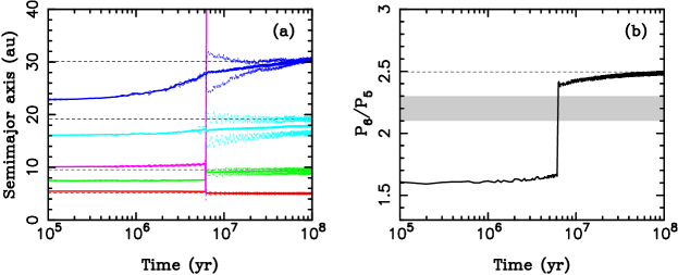
Figure 3: Orbital histories of the giant planets from NM12. Five planets were started in the (3:2,4:3,2:1,3:2) resonant chain, and $M_{\rm disk}=20$ $M_{\oplus}$. (a) The semimajor axes (solid lines), and perihelion and aphelion distances (dashed lines) of each planet’s orbit. The horizontal dashed lines show the semimajor axes of planets in the present Solar System. The final orbits obtained in the model, including $e_{\rm 55}$, are a good match to those in the present Solar System. (b) The period ratio $P_{6}/P_{5}$. The dashed line shows $P_{6}/P_{5}=2.49$ corresponding to the present orbits of Jupiter and Saturn. The shaded area approximately denotes the zone, where the secular resonances with the terrestrial planets and asteroids occur. These resonances are not activated, because the period ratio ‘jumps’ over the shaded area as Jupiter and Saturn scatter off of the ejected ice giant.

NM12 defined four criteria to measure the overall success of their simulations. First of all, the final planetary system must have four giant planets (criterion A) with orbits that resemble the present ones (criterion B). Note that A means that one and two planets must be ejected in the five- and six-planet planet cases, while all four planets must survive in the four-planet case. As for B, success was claimed if the final semimajor axis of each planet was within 20% to its present value, and the final eccentricities and inclinations were no larger than 0.11 and 2^∘, respectively. These thresholds were obtained by doubling the current mean eccentricity of Saturn ($e_{6}=0.054$) and mean inclination of Uranus ($i_{7}=1.02^{\circ}$). NM12 also required that $e_{55}>0.022$, i.e., at least half of its current value (criterion C; see discussion in Section 4). Moreover, the $P_{\rm 6}/P_{\rm 5}$ ratio was required to evolve from $<$2.1 to $>$2.3 in $\ll$ 1 Myr (Criterion D), as needed to satisfy the terrestrial planet and asteroid belt constraints (Sections 7 and 8). The terrestrial planets and asteroids were not explicitly included in NM12 to speed up the calculations.

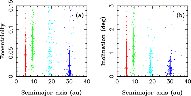
Figure 4: Final planetary orbits obtained in 500 simulations with five outer planets started in the (3:2,3:2,2:1,3:2) resonant chain and $M_{\rm disk}=20$ M_⊕. The mean orbital elements were obtained by averaging the osculating orbital elements over the last 10 Myr of the simulation. Only the systems ending with four outer planets are plotted here (dots). The bars show the mean and standard deviation of the model distribution of orbital elements. The mean orbits of real planets are shown by triangles. Colors red, green, turquoise and blue correspond to Jupiter, Saturn, Uranus and Neptune.

Figure 3 shows an example of a successful simulation that satisfied all four criteria. This is a classical example of the jumping-Jupiter model. The instability happened in this case about 6 Myr after the start of the simulation. Before the instability, the three ice giants slowly migrated by scattering planetesimals. The instability was triggered when the inner ice giant crossed an orbital resonance with Saturn and its eccentricity was pumped up. Following that, the ice giant had encounters with all other planets, and was ejected from the Solar System by Jupiter. Jupiter was scattered inward and Saturn outward during the encounters, with $P_{6}/P_{5}$ moving from $\simeq$1.7 to $\simeq$2.4 in less that $10^{5}$ yr (Figure 3b). The orbits of Uranus and Neptune became excited as well, with Neptune reaching $e_{8}\simeq 0.15$ just after the instability ($e_{8}\simeq 0.05$-0.15 in all successful models from NM12). The orbital eccentricities were subsequently damped by dynamical friction from the planetesimal disk. Uranus and Neptune, propelled by the planetesimal-driven migration, reached their current orbits some 100 Myr after the instability. The final eccentricities of Jupiter and Saturn were $e_{5}=0.031$ (modal amplitude $e_{55}=0.030$) and $e_{6}=0.058$. For comparison, the mean eccentricities of the real planets are $e_{5}=0.046$ and $e_{6}=0.054$.

NM12 found (see also Nesvorný 2011, Batygin et al. 2012, Deienno et al. 2017) that the dynamical evolution is typically too violent, if planets start in a compact resonant configuration, leading to ejection of at least one ice giant from the Solar System. Planet ejection could be avoided for large masses of the outer planetesimal disk ($M_{\rm disk}>50$ $M_{\oplus}$), but a massive disk would lead to excessive dynamical damping (Figure 1b) and migration regime that violates various constraints (e.g., Section 11). The dynamical simulations starting with a resonant system of four giant planets thus have a very low success rate. In fact, NM12 have not found any case that would satisfy all four criteria in nearly 3000 simulations of the four planet case. Thus, either the Solar System followed an unusual evolution path ($<$1/3000 probability to satisfy criteria A-D), some constraints are misunderstood, or there were originally more than four planets in the outer Solar System.

Better results were obtained in NM12 when the Solar System was assumed to have five giant planets initially and one ice giant, with the mass comparable to that of Uranus and Neptune, was ejected into interstellar space by Jupiter (Figure 3). The best results were obtained when the ejected planet was placed into the external 3:2 or 4:3 resonance with Saturn and $M_{\rm disk}\simeq 15$-20 M_⊕. The range of possible outcomes is rather broad in this case (Figure 4), indicating that the present Solar System is neither a typical nor expected result for a given initial state, and occurs, in best cases, with a $\simeq$5% probability (as defined by the NM12 success criteria). [If it is assumed that each of the four NM12 criteria is satisfied in 50% of cases, and the success statistics are uncorrelated, the expectation is $0.5^{4}=0.063$, or 6.3%.]

[SUMMARY] In summary of Sections 2-5, the planetesimal-driven migration explains how Uranus and Neptune evolved from their initially more compact orbits. Neptune’s migration, in particular, is badly needed to understand the orbital structure of the Kuiper belt, where orbital resonances with Neptune are heavily populated (Section 11). The planetesimal-driven migration, when applied to Jupiter and Saturn, leads to an impasse, because it does not explain why Jupiter’s present eccentricity (and specifically the $e_{55}$ mode) is significant. The planetesimal-driven migration of Jupiter and Saturn also generates incorrect expectations for the terrestrial planet AMD and the orbital structure of the asteroid belt.

The dynamical instability in the outer Solar System, followed by encounters of an ice giant with all other outer planets, offers an elegant solution to these problems. The scattering encounters excite the orbital eccentricities and inclinations of the outer planets (including the $e_{55}$ mode). As a result of the scattering encounters, Jupiter jumps inward and Saturn outward. The inner Solar System constraints are not violated in this case. The jumping-Jupiter model is the most easily accomplished if there initially was a third ice giant planet, with mass comparable to that of Uranus or Neptune, on a resonant orbit between Saturn and Uranus. The orbit of the hypothesized third ice giant was destabilized during the instability and the planet was subsequently ejected into interstellar space by Jupiter.

6 GIANT PLANET OBLIQUITIES

The obliquity, $\theta$, is the angle between the spin axis of an object and the normal to its orbital plane. Here we consider the obliquities of Jupiter and Saturn. The core accretion theory applied to Jupiter and Saturn implies that their primordial obliquities should be small. This is because the angular momentum of the rotation of these planets is contained almost entirely in their massive hydrogen and helium envelopes. The stochastic accretion of solid cores should therefore be irrelevant for their current obliquity values, and a symmetric inflow of gas on forming planets should lead to $\theta=0$. The present obliquity of Jupiter is $\theta_{5}=3.1^{\circ}$, which is small enough to be roughly consistent with these expectations, but that of Saturn is $\theta_{6}=26.7^{\circ}$, which is not.

It has been noted (Ward & Hamilton 2004, Hamilton & Ward 2004) that the precession frequency of Saturn’s spin axis, $p_{6}=-\alpha_{6}\cos\theta_{6}$, where $\alpha_{6}$ is Saturn’s precessional constant (a function of the quadrupole gravitational moment, etc.), has a value close to $s_{8}=-0.692$ arcsec yr^-1, where $s_{8}$ is the 8th nodal eigenfrequency of the planetary system (Section 7). Similarly, Ward & Canup (2006) pointed out that $p_{5}=-\alpha_{5}\cos\theta_{5}\simeq s_{7}$, where $\alpha_{5}$ is Jupiter’s precessional constant, and $s_{7}=-2.985$ arcsec yr^-1.

While it is not clear whether the spin states of Jupiter and Saturn are actually in the spin-orbit resonances at the present (e.g., the current best estimate for Saturn is $|p_{6}|=0.75$ arcsec yr^-1, Helled et al. 2009), the similarity of frequencies is important, because the spin-orbit resonances can excite $\theta$. This works as follows. There are several reasons to believe that $\alpha_{6}/s_{8}$ has not remained constant since Saturn’s formation. For example, it has been suggested that $|\alpha_{6}/s_{8}|<1$ initially, and then evolved to $|\alpha_{6}/s_{8}|=1$, when $\alpha_{6}$ increased as a result of Saturn’s cooling and contraction, or because $s_{8}$ decreased during the depletion of the primordial Kuiper belt. If so, the present obliquity of Saturn could be explained by capture of Saturn’s spin vector in the $p_{6}=s_{8}$ resonance, because the resonant dynamics can compensate for the slow evolution of $\alpha_{6}/s_{8}$ by boosting $\theta_{6}$ (Ward & Hamilton 2004).

While changes of $\alpha_{6}/s_{8}$ during the earliest epochs could have been important, it seems more likely that capture in the spin-orbit resonance occurred later, probably as a result of planetary migration. This is because both $s_{7}$ and $s_{8}$ significantly change during the planetary migration and dispersal of the outer disk. Therefore, if the spin-orbit resonances had been established earlier, they would not survive to the present time. Boué et al. (2009) studied various models for tilting Saturn’s spin axis during planetary migration and found that the present obliquity of Saturn can be explained by resonant capture if the characteristic migration time scale was long and/or Neptune reached high orbital inclination during the instability.

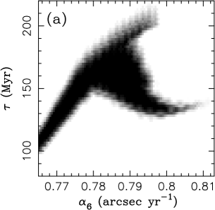
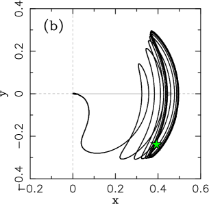
Figure 5: Left: Saturn obliquity constrain on the planetary migration timescale $\tau$ and precession constant $\alpha_{6}$. Different $\tau$ and $\alpha_{6}$ values were tested to see how they affect the excitation of Saturn’s obliquity in the $p_{6}=s_{8}$ spin-orbit resonance. The dark region highlights the parameter values which resulted in $\theta_{6}\simeq 27^{\circ}$ and simultaneously provided a sufficiently large libration amplitude ($>$$30^{\circ}$) in the resonance to explain the orientation of Saturn’s spin vector. Right: Example of Saturn’s obliquity excitation for $\alpha_{6}=0.785$ arcsec yr^-1 and $\tau=150$ Myr. The spin axis $\mathbf{s}$ is projected onto $(x,y)$ plane, where $x=\sin\theta\cos\varphi$ and $y=\sin\theta\sin\varphi$, and $\varphi$ defines the azimuthal orientation of $\mathbf{s}$. The arrow shows the evolution of the Cassini state $C_{2}$ over the whole length of the simulation (1 Gyr). The present orientation of Saturn’s spin vector in the $(x,y)$ plane is denoted by the green star. Figures from VN15.

In fact, the obliquities of Jupiter and Saturn represent a stronger constraint on the instability/migration models than was realized before. This is because they must be satisfied simultaneously (Brasser & Lee 2015). For example, in the initial compact configurations of the Nice model, the $s_{8}$ frequency is much faster than both $\alpha_{5}$ and $\alpha_{6}$. As $\alpha_{5}>\alpha_{6}$, this means that $s_{8}$ should first cross $\alpha_{5}$ to reach $\alpha_{6}$ during the subsequent evolution. This leads to a conundrum, because if the crossing were slow, $\theta_{5}$ would increase as a result of capture into the spin-orbit resonance with $s_{8}$. If, on the other hand, the evolution were fast, the conditions for capture of $\theta_{6}$ into the spin-orbit resonance with $s_{8}$ would not be met (Boué et al. 2009), and $\theta_{6}$ would stay small.

A potential solution of this problem is to invoke fast evolution of $s_{8}$ at the $s_{8}=-\alpha_{5}$ crossing, and slow evolution of $s_{8}$ at the $s_{8}=-\alpha_{6}$ crossing. This can be achieved, for example, if the migration of outer planets was relatively fast initially, and slowed down later, as planets converged to their current orbits. Vokrouhlický & Nesvorný (2015; hereafter VN15) documented this possibility in the jumping-Jupiter models developed in NM12. Recall from Section 5 that the most successful NM12 models feature two-stage migration histories with $\tau_{1}\sim 10$ Myr before the instability and $\tau_{2}\sim 30$-50 Myr after the instability. Moreover, the migration tends to slow down relative to a simple exponential at very late stages (effective $\tau\geq 100$ Myr).

VN15 found that Saturn’s obliquity can indeed be excited by capture in the $p_{6}=s_{8}$ spin-orbit resonance (Ward & Hamilton 2004, Hamilton & Ward 2004, Boué et al. 2009) during the late stages of planetary migration. To reproduce the current orientation of Saturn’s spin vector, however, specific conditions must be met (Figure 5). First, Neptune’s late-stage migration must be slow with $100<\tau<200$ Myr. Fast migration rates with $\tau<100$ Myr do not work because the resonant capture and excitation of $\theta_{6}$ do not happen. Second, for Saturn to remain in the $p_{6}=s_{8}$ resonance today, $\alpha_{6}<0.8$ arcsec yr^-1, which is lower than the estimate derived from modeling of Saturn’s interior ($\alpha_{6}=0.845$ arcsec yr^-1; Helled et al. 2009). Interestingly, direct measurements of the mean precession rate of Saturn’s spin axis suggest $\alpha_{6}=0.81\pm 0.05$ arcsec yr^-1 (see discussion in VN15), which would allow for $\alpha_{6}<0.8$ arcsec yr^-1 within the quoted uncertainty.

As for Jupiter, the $p_{5}=s_{8}$ resonance occurs during the first migration stage of NM12. To avoid resonant capture and excessive excitation of $\theta_{5}$, either ${\rm d}s_{8}/{\rm d}t$ must be large or $i_{58}$ must be small, where $i_{58}$ is the amplitude of the $s_{8}$ term in the Fourier expansion of Jupiter’s orbital precession. There are good reasons to believe that $i_{58}$ during the first migration stage was small, and likely smaller than the current value ($i_{58}\simeq 0.05^{\circ}$). If so, ${\rm d}s_{8}/{\rm d}t>0.05$ arcsec yr^-1 Myr^-1 would imply that the crossing of $p_{5}=s_{8}$ happened fast enough such that Jupiter’s obliquity remained low ($\theta_{5}<3^{\circ}$; VN15). For comparison, ${\rm d}s_{8}/{\rm d}t\sim 0.1$ arcsec yr^-1 Myr^-1 during the first migration stage in NM12. This shows that the NM12 model does not violate the Jupiter obliquity constraint.

To obtain $\theta_{5}\simeq 3^{\circ}$ from the $p_{5}=s_{8}$ resonance crossing, $i_{58}$ would need to be significant. For example, assuming that $i_{58}=0.025^{\circ}$, i.e. about half of its current value, a very slow migration rate with ${\rm d}s_{8}/{\rm d}t\simeq 0.014$ arcsec yr^-1 Myr^-1 would be required (VN15), which is well below the expectation from the NM12 model. It thus seems more likely that Jupiter’s obliquity emerged when $p_{5}$ approached $s_{7}$ near the end of planetary migration (Ward & Canup 2006). For that to work, however, the precession constant $\alpha_{5}$ would have to be significantly larger than $\alpha_{5}=2.77$ arcsec yr^-1 suggested by Helled et al. (2011). For example, if $\theta_{5}<1^{\circ}$ before the system approached the $p_{5}=s_{7}$ resonance, then $\alpha_{5}=2.93$-2.95 arcsec yr^-1 would be needed to obtain $\theta_{5}\simeq 3^{\circ}$ (VN15). This constitutes an interesting prediction that will be testable by the Juno mission.

7 TERRESTRIAL PLANETS

The principal interaction between the terrestrial and giant planets during planetary migration occurs through their secular coupling. In brief, for a non-resonant system of planets with masses $m_{i}$ and semimajor axes $a_{i}$, where index $i$ goes from 1 (Mercury) to 8 (Neptune), the secular coupling can be described by the Laplace-Lagrange equations. Denoting $(h_{i},k_{i})=e_{i}(\sin\varpi_{i},\cos\varpi_{i})$, where $e_{i}$ and $\varpi_{i}$ are the eccentricity and perihelion longitude of the $i$th planet, the Laplace-Lagrange equations admit general solutions with $h_{i}=\Sigma_{j}e_{ij}\sin(g_{j}t+\phi_{j})$ and $k_{i}=\Sigma_{j}e_{ij}\cos(g_{j}t+\phi_{j})$, where $g_{j}$ are eight eigenfrequencies, and $e_{ij}$ and $\phi_{j}$ are the amplitudes and phases that can be obtained by solving an eigenvalue problem. Similarly, defining $(q_{i},p_{i})=i_{i}(\sin\Omega_{i},\cos\Omega_{i})$, where $i_{i}$ and $\Omega_{i}$ are the inclination and nodal longitude with respect to the invariant plane, it can be shown that $q_{i}=\Sigma_{j}i_{ij}\sin(s_{j}t+\psi_{j})$ and $p_{i}=\Sigma_{j}i_{ij}\cos(s_{j}t+\psi_{j})$, where $s_{j}$, $i_{ij}$ and $\psi_{j}$ are eigenfrequencies, amplitudes and phases.

When considering the secular evolution of an isolated system, the semimajor axes of planets are constant, and the total angular momentum is conserved. The Angular Momentum Deficit (AMD), defined as ${\rm AMD}=\Sigma_{i}m_{i}n_{i}a_{i}^{2}(1-(1-e_{i}^{2})^{1/2}\cos i_{i})$, where $n_{i}$ is the orbital frequency of the $i$th planet, is an integral of motion (Laskar 1996). It physically corresponds to the angular momentum that needs to be added to make all orbits perfectly circular and coplanar. Using the solution of the Laplace-Lagrange equations discussed above, AMD can be partitioned into conserved quantities $C_{j}$ and $D_{j}$ that describe the distribution of the AMD among different eccentricity and inclinations modes of each planet (Agnor & Lin 2012, hereafter AL12). Moreover, the modal amplitudes $C_{j}$ and $D_{j}$ are constant if $a_{j}$ change slowly, except if the system evolves near a secular resonance such that $g_{j}-g_{k}=0$ or $s_{j}-s_{k}=0$.

When a secular resonance occurs, the partitioning of the AMD between different modes may change. Because there is much more AMD in modes with $j\geq 5$ than in $j\leq 4$ (mainly due to the large masses of the outer planets), Jupiter and Saturn represent a practically unlimited source of AMD that, if even partially transferred to the terrestrial planets, will make their orbits very eccentric and inclined. The orbits could then cross each other, leading to collisions between the terrestrial planets.

These considerations constrain the evolution of the secular modes of the outer planets, mainly $g_{5}$, from their effects on the terrestrial planets. For example, using the initial configuration of planets from Hahn & Malhotra (1999), $P_{\rm 6}/P_{\rm 5}=2.06$, where $P_{\rm 5}$ and $P_{\rm 6}$ are the orbital periods of Jupiter and Saturn. The initial orbits are therefore just wide of the 2:1 resonance, and $g_{5}>g_{1}$ and $g_{5}>g_{2}$ (e.g., Fig. 4 in AL12). The present value of $g_{5}$ is 4.24 arcsec yr^-1, while $g_{1}=5.86$ arcsec yr^-1 and $g_{2}=7.42$ arcsec yr^-1. Therefore, $g_{5}<g_{1}$ and $g_{5}<g_{2}$ in the present Solar System. This means that the $g_{1}=g_{5}$ and $g_{2}=g_{5}$ resonances must be crossed. The same resonances occur in the original Nice model (Tsiganis et al. 2005), but their consequences for the terrestrial planets were not understood in 2005.

More recent studies show that the slow crossing of the secular resonances would produce excessive excitation and instabilities in the terrestrial planet system (AL12, Brasser et al. 2009). For example, starting from the initial $e_{22}=0.01$, and requiring that the final $e_{22}<0.03$ (the present value is $e_{22}=0.018$), AL12 did not find any cases that would satisfy this constraint if the assumed characteristic migration timescale $\tau>0.15$ Myr. In contrast, the timescale of planetesimal-driven migration is much longer, with the most quoted values $\tau\geq 5$ Myr (e.g., Hahn & Malhotra 1999, Gomes et al. 2004, Tsiganis et al. 2005, NM12, Nesvorný 2015a). This problem could be resolved if $e_{55}\simeq 0$, because the strength of the secular resonances involving the $g_{5}$ frequency scales with the amplitude $e_{55}$, but this would not work either, because it would leave unexplained why $e_{55}=0.044$ now.

Figure 6: Excitation of Mercury’s eccentricity (left) and inclination (right) during the dynamical instability in the outer Solar System. The orbits of outer planets are shown in Figure 3. The instability happened about 6 Myr after the start of the simulation. The initial AMD of the terrestrial planets was assumed to be zero. During the instability, $e_{1}$ was excited by the $g_{1}=g_{5}$ resonance and $i_{1}$ was excited by the $s_{1}=s_{7}$ resonance (Roig et al. 2016). The final mean eccentricity and mean inclination were 0.16 and 6.3^∘, in a good match to the present orbit of Mercury.

As $g_{5}$ is mainly a function of the orbital separation between Jupiter and Saturn, the constraints from the terrestrial planets can be approximately defined in terms of $P_{\rm 6}/P_{\rm 5}$. According to AL12, this ratio needs to evolve from $<$2.1 to $>$2.3 in $<$0.15 Myr, which can be achieved, for example, if planetary encounters with an ice giant scattered Jupiter inward and Saturn outward (Brasser et al. 2009). This condition has been used to measure the success of the instability simulations in NM12 to identify promising cases, which should not violate the terrestrial planet constraint. In fact, NM12’s criterion on $P_{\rm 6}/P_{\rm 5}$ is only a rough expression of the terrestrial planet constraint. AL12 showed that even if the migration is very rapid ($\tau=0.1$ Myr), there is still only a $\simeq$40% chance that the final $e_{22}<0.03$ (assuming constant $e_{55}=0.0443$). A question therefore arises whether the NM12 models are truly consistent with the terrestrial planet constraint, or not.

Roig et al. (2016) tested several cases from NM12 (see also Brasser et al. 2013), including the one shown in Figure 3. The selected cases were required to pass the NM12 criterion on $P_{\rm 6}/P_{\rm 5}$ (Section 5). The terrestrial planets were explicitly included in their $N$-body integrations. The initial AMD of the terrestrial planet system was assumed to be much lower than the present one to test whether gravitational perturbations from the outer planet system can be responsible for the modestly excited orbits of the terrestrial planets.

The results are interesting. In some cases, the eccentricities and inclinations of the terrestrial planets become excited to values similar to the present ones. For example, the excitation by $g_{1}=g_{5}$ and $s_{1}=s_{7}$ resonances can explain why Mercury’s orbital eccentricity and inclination are large (mean $e_{1}=0.17$ and mean $i_{1}=7^{\circ}$; Figure 6). The Mars’s inclination is not excited enough perhaps indicating that Mars acquired its inclined orbit (mean $i_{4}\simeq 4.5^{\circ}$) before the planetary migration/instability. In other cases, the simulations failed because the planetary orbits were excited too much (Roig et al. 2016).

Kaib & Chambers (2016) emphasized the low probability that the terrestrial planet system remains unchanged during the planetary migration/instability. With the 5-planet model from NM12 and the outer planets starting in the (3:2,3:2,2:1,3:2) resonant chain, they found that all terrestrial planet survive in only $\sim$2% of trials and the AMD generated by the planetary migration/instability does not exceed the current one in only $\sim$1% of trials. This is roughly consistent with the previous work, because NM12 found that the $P_{6}/P_{5}$ criterion was satisfied in $\sim$5% of cases, and Roig et al. (2016) showed that only some of these cases actually satisfy the terrestrial planet constraint.

The low probability of matching the terrestrial planet constraint is worrisome. The terrestrial planet region may have contained additional planets, either inside the orbit of Venus or outside of Earth’s orbit. A planet inside Venus’s orbit would presumably be excited together with Mercury, and its collision with Mercury would probably ensue. The collision could reduce the AMD of the terrestrial planets and lead to better results. A hit-and-run collision was previously suggested to explain why Mercury looks like a iron core of a larger planet (Asphaug & Reufer 2014). The most straightforward solution to this problem, however, is to assume that the planetary migration/instability happened early, within $\sim$50 Myr after the dispersal of the protoplanetary gas disk (Section 13). If so, the terrestrial planet formation was not completed and the architecture of the terrestrial planet zone may have been radically different.

8 ASTEROID BELT

The orbital distribution of main belt asteroids is carved by resonances. This happens because resonant dynamics generally increase orbital eccentricities, lead to planet-crossing orbits, and thus tend to remove bodies evolving into resonances (the Hilda asteroids in the 3:2 orbital resonance with Jupiter are a notable exception). More specifically, the $g=g_{6}$ and $s=s_{6}$ resonances (also known as $\nu_{6}$ and $\nu_{16}$), where $g$ and $s$ are the precession frequencies of the proper perihelion and proper nodal longitudes of an asteroid, fall near the current inner boundary of the asteroid belt ($a\simeq 2$ au for low-inclination orbits; Figure 7). The excitation of eccentricities and inclinations in these resonances occurs by processes closely analogous to those discussed in Section 7. The orbital resonances, on the other hand, such as 2:1, 3:1, 5:2 and 7:3 with Jupiter (e.g., the 2:1 resonance occurs when the orbital period, $P$, is exactly a half of Jupiter’s period; $P=11.8/2=5.9$ yr), lead to amplified variations of the eccentricity on resonant and secular timescales. The semimajor axis values where the resonances occur correspond to gaps in the orbital distribution of asteroids, known as the Kirkwood gaps.

In the early Solar System, when the planetary orbits were different (Sections 2-5), the asteroidal resonances were at different locations than they are now. For example, with Jupiter on an initial orbit with $a_{5}\simeq 5.8$ au (NM12), the 3:1 resonance was at $\simeq$2.8 au, from where it must have moved inwards over the central part of the main belt to reach its current location at 2.5 au. Other orbital resonances shifted as well. With Jupiter and Saturn in a compact configuration with $P_{6}/P_{5}<2.1$, the $\nu_{6}$ resonance started beyond 4 au, from where it must have moved over the whole asteroid belt to $a\simeq 2$ au (for $i\sim 0$) when the orbits of Jupiter and Saturn reached their current orbital period ratio ($P_{6}/P_{5}=2.49$).

To understand this issue, various studies considered the planetesimal-driven migration (Section 2). The studies used artificial force terms to induce smooth planetary migration from the initial orbits and placed limits on the migration timescale. For example, it has been suggested that an exponential migration $a(t)=a_{0}+\Delta a[1-\exp(-t/\tau)]$, where $a_{0}$ is the initial semimajor axis, $\Delta a$ is the migration distance ($\Delta a=-0.2$ au for Jupiter and $\Delta a=0.8$ au for Saturn), and $\tau\simeq 0.5$ Myr can explain the semimajor axis distribution of main belt asteroids (Minton & Malhotra 2009). In addition, assuming $\tau\geq 5$ Myr, which is more consistent with the timescale expected from the planetesimal-driven migration (Section 11), the sweeping $\nu_{16}$ resonance would excite orbital inclinations to $i>20^{\circ}$, while inclinations $i>20^{\circ}$ are rare in the present main belt (Morbidelli et al. 2010, Toliou et al. 2016).

Figure 7: Left: The orbital distribution of main belt asteroids with diameters $D>30$ km. The smaller dots for $a<2$ au highlight Hungarias, which are thought to be a remnant of the E-belt (Bottke et al. 2012). Since Hungarias are all smaller than 30 km, here we plot known asteroids with $a<2$ au and $D>5$ km. The higher density of orbits at $a\simeq 3.1$-3.2 au is a consequence of collisional breakups of several large asteroids in this region (e.g., Themis and Eos families). Right: The distribution of orbits obtained in the jumping-Jupiter model (Nesvorný et al. 2017b). The initial inclination distribution was assumed to extend to $i=20^{\circ}$. The solid lines denote the secular resonances $\nu_{6}$ ($g=g_{6}$) and $\nu_{16}$ ($s=s_{6}$). The dashed lines in (a) and (c) is where the orbits become Mars crossing.

The results discussed above therefore imply a very short migration timescale. In this respect, the asteroid belt constraint is similar to that obtained from the terrestrial planets (Section 7), except that it applies even if planetary migration/instability occurred early.

Very short migration timescales are difficult to obtain from the planetesimal-driven migration, because that would require a very massive planetesimal disk (Hahn & Malhotra 1999) and would extract AMD from the outer planets, leaving them on more circular orbits than they have now. Instead, it has been suggested that the asteroid constraint can be satisfied in the jumping-Jupiter model, where $P_{\rm 6}/P_{\rm 5}$ changes in discrete steps with each step corresponding to an encounter of Jupiter or Saturn with an ice giant (Morbidelli et al. 2010; Section 4). In an idealized version of this model, when Jupiter and Saturn are assumed to be instantaneously transported from the 3:2 (or 2:1) resonance to their present orbits, the $\nu_{6}$ and $\nu_{16}$ resonances step over the main belt and leave the original orbital distribution of asteroids practically unchanged.

The reality is more complicated. Self-consistent simulations of the jumping-Jupiter model show that the radial transport of planetary orbits is not executed in a single encounter. Instead, both Jupiter and Saturn experience many encounters with an ice giant during a period lasting 50,000 to 300,000 years (NM12). The orbital and secular resonances move in a number of discrete steps over the main belt region and can affect asteroid orbits. As for the orbits with $a>2.5$ au, the jumping resonances are found to excite orbital eccentricities; inclinations are affected less (Roig & Nesvorný 2015). As for $a<2.5$ au, where both $\nu_{6}$ and $\nu_{16}$ spend more time, the original population is depleted (by a factor of $\sim$10 for $2.1<a<2.5$ au). This can explain why the inner part of the belt with $2.1<a<2.5$ au represents only $\sim$1/10 of the total main belt population (Figure 7). Overall, the main belt loses $\sim$80% of its original population (Minton & Malhotra 2010, Nesvorný et al. 2017b). The population loss is not large enough to explain the low mass of the main belt ($\simeq$$5\times 10^{-4}$ $M_{\oplus}$) when compared to the expectation based on the radial interpolation of the surface density of solids between the terrestrial planets and Jupiter’s core (Weidenschilling 1977).

In the jumping-Jupiter models investigated so far, the dynamical effects on the orbital eccentricities and inclinations are not large enough to explain the general excitation of the asteroid belt (Roig & Nesvorný 2015). The processes that excited the belt from the dynamically cold state (that must have prevailed during the accretion epoch) therefore most likely predate the planetary migration/instability (Morbidelli et al. 2015). For example, the asteroid belt may have become excited (and depleted) before the dispersal of the protoplanetary gas disk if Jupiter temporarily moved into the main belt region and scattered asteroids around (the GT model; Walsh et al. 2011). In fact, the GT model is known to produce a very broad eccentricity distribution (mean $e\sim 0.3$-0.4 compared to the present mean $e\sim 0.1$). This is not a problem, however, because it has been shown that the subsequent dynamical erosion of orbits with $e>0.2$ leads to a narrower eccentricity distribution that is more similar to the observed one (Deienno et al. 2016).

Asteroids can be grouped into taxonomic classes based on their reflectance properties. The S-type asteroids show absorption features similar to the ordinary chondrite meteorites, which are rich in silicates. They are thought to have formed in the main belt region. The C-type asteroids have featureless neutral spectrum and are likely related to carbonaceous chondrites. They are predominant in the central and outer parts of the main belt (2.5-3.3 au) and are thought to be interlopers from the Jupiter-Saturn zone (Walsh et al. 2011, Kruijer et al. 2017). The Cybele asteroids at 3.3-3.7 au, the Hilda asteroids in the 3:2 resonance with Jupiter ($\simeq$3.9 au), and Jupiter Trojans are mainly P- (less red spectral slope) and D-types (redder slope). Since Jupiter Trojans are thought to have been captured from the outer disk of planetesimals ($a>20$ au; Section 9), the P- and D-type classes are probably related to H₂0-ice rich comets that formed beyond 20 au. Studies show that the outer disk planetesimals can be captured not only as Jupiter Trojans, but also as Hildas, Cybeles and in the main belt below 3 au (Levison et al. 2009, Vokrouhlický et al. 2016).

The fifth planet helps to increase the implantation efficiency into the inner part of the main belt (Vokrouhlický et al. 2016), where several small P-/D- type asteroids were found (DeMeo et al. 2015). The mean probability for each outer-disk body to be implanted into the asteroid belt at 2-3.2 au was estimated to be $\sim 5\times 10^{-6}$ (Vokrouhlický et al. 2016). This is consistent with the number of large P-/D-type bodies in the belt ($D>150$ km), but represents a significant excess over the estimated population of smaller P-/D-types. This problem can be attributed to some physical process that has not been included in the existing dynamical studies (thermal or volatile-driven destruction of small P-/D-types during their implantation below 3 au, their subsequent collisional destruction, etc.).

9 JUPITER TROJANS

Jupiter Trojans are a population of small bodies with orbits near that of Jupiter. They hug two equilibrium points of the three-body problem, known as $L_{4}$ and $L_{5}$, with $a\simeq a_{5}=5.2$ au, $e<0.15$, $i<40^{\circ}$, and $\delta\lambda=\lambda-\lambda_{5}\sim\pm 60^{\circ}$, where $\lambda$ and $\lambda_{5}$ are the mean longitudes of Trojan and Jupiter. The angle $\delta\lambda$ librates with a period of $\sim$150 yr and full libration amplitude, $D$, up to $D\simeq 70^{\circ}$. The color distribution of Jupiter Trojans is bimodal with $\sim$80% of the classified bodies in the red group (red slope similar to that of D types in asteroid taxonomy) and $\sim$20% in the less red group (similar to P types). The distribution of visual albedo is uniform with typical values $\simeq$5-7% (Grav et al. 2011), indicating some of the darkest surfaces in the Solar System.

Morbidelli et al. (2005, hereafter M05) proposed that Jupiter Trojans were trapped in orbits at $L_{4}$ and $L_{5}$ by chaotic capture. Chaotic capture takes place when Jupiter and Saturn pass, during their orbital migration, near the mutual 2:1 resonance, where the period ratio $P_{\rm 6}/P_{\rm 5}\simeq 2$. The angle $\lambda_{\rm 5}-2\lambda_{\rm 6}-\varpi$, where $\varpi$ is the mean longitude of either Jupiter or Saturn, then resonates with $\delta\lambda$, creating widespread chaos around $L_{4}$ and $L_{5}$. Small bodies scattered by planets into the neighborhood of Jupiter’s orbit can chaotically wander near $L_{4}$ and $L_{5}$, where they are permanently trapped once $P_{\rm 6}/P_{\rm 5}$ moves away from 2. A natural consequence of chaotic capture is that orbits fill all available space characterized by long-term stability, including small libration amplitudes and large inclinations.

This model resolves a long-standing conflict between previous formation theories that implied $i<10^{\circ}$ (see Marzari et al. 2002 and the references therein) and observations that show orbital inclinations up to 40^∘. Attempts to explain large inclinations of Trojans by exciting orbits after capture have been unsuccessful, because passing secular resonances and other dynamical effects are not strong enough (e.g., Marzari & Scholl 2000).

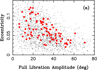
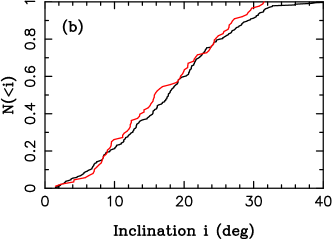
Figure 8: Left: Orbits of stable Jupiter Trojans obtained in the jumping-Jupiter simulations in NVM13 (red dots). The full libration amplitude $D$ corresponds to the angular distance between extremes of $\lambda-\lambda_{5}$ during libration. The black dots show the orbital distribution of known Trojans. Right: Cumulative inclination distribution of known Jupiter Trojans with absolute magnitude $H<12$ (black line; the $H$ cut is done to limit the effect of the observational bias) and bodies captured in the NVM13 model (red line).

M05 placed chaotic capture in the context of the original Nice model (Tsiganis et al. 2005). As we explained in Section 4, however, it is now thought that Jupiter and Saturn have not smoothly migrated over the 2:1 resonance. Instead, $P_{6}/P_{5}$ probably changed from $<$2 to $>$2.3 when Jupiter/Saturn scattered off of an ice giant. M05’s chaotic capture does not work in the jumping-Jupiter model, because the resonances invoked in M05 do not occur.

In a follow-up work, Nesvorný, Vokrouhlický & Morbidelli (2013, hereafter NVM13) tested capture of Jupiter Trojans in the jumping-Jupiter model. They found that a great majority of Trojans were captured immediately after the closest encounter of Jupiter with an ice giant. As a result of the encounter, $a_{5}$ changed, sometimes by as much as $\sim$0.2 au in a single jump. This radially displaced Jupiter’s $L_{4}$ and $L_{5}$, released the existing Trojans, and led to capture of new bodies that happened to have semimajor axes similar to $a_{5}$ when the jump occurred. NVM13 called this jump capture. The chaotic capture, arising from the proximity of Jupiter and Saturn to the 5:2 resonance, was estimated to contribute only by $\sim$10-20% to the present population of Jupiter Trojans (NVM13).

In principle, both the chaotic and jump capture can produce Trojans from any source reservoir that populated Jupiter’s region at the time when the orbit of Jupiter changed. For example, planetesimals from the outer disk can be scattered to $\sim$5 au via encounters with the outer planets. The massive outer disk ($M_{\rm disk}\simeq 15$-20 $M_{\oplus}$) also represents a large source reservoir. Both M05 and NVM13 therefore found that an overwhelming majority of Jupiter Trojans were captured from the outer disk. The asteroid contribution to Jupiter Trojans is negligible (Roig & Nesvorný 2015).

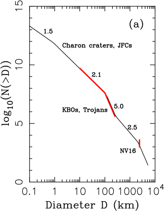
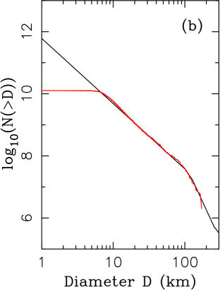
Figure 9: The calibrated size distribution of the original planetesimal disk below 30 au (panel a). The red color denotes various constraints. The distribution for $10<D<300$ km was inferred from observations of Jupiter Trojans and KBOs, and from the Jupiter Trojan capture probability determined in NVM13. Panel (b) zooms in on the distribution of $1<D<250$ km planetesimals. The red line in panel (b) shows the size distribution of known Jupiter Trojans (the sample is incomplete for $D<10$ km). The existence of 1000-4000 Plutos in the original disk inferred in Nesvorný & Vokrouhlický (2016; labeled as NV16 in panel a) requires that the size distribution had a hump at $D>300$ km. The numbers above the reconstructed size distribution in panel (a) show the cumulative power index that was used for different segments. The total mass of the disk, here $M_{\rm disk}=20$ $M_{\oplus}$, is dominated by $\simeq$100-km-class bodies.

The orbital distribution of stable Trojans produced in the NVM13 simulations very closely matches observations (Figure 8). The distribution extends down to very small libration amplitudes, small eccentricities and small inclinations. These orbits are generally the most difficult to populate in any capture model. The inclination distribution of captured objects is wide, reaching beyond 30^∘, just as needed. In the best case, the Kolmogorov-Smirnov test (Press et al. 1992) gives 60%, 68% and 63% probabilities that the simulated and known distributions of $D$, $e$ and $i$ are statistically the same. The capture probability (as a stable Trojan) was found to be $P=(5\pm 3)\times 10^{-7}$ for each particle in the original planetesimal disk, where the error expresses the full range of results obtained in the jumping-Jupiter models tested so far.

Since the capture process is size independent, the size frequency distribution (SFD) of Trojans should be a scaled-down version of the transplanetary disk’s SFD. After capture, the Trojan population underwent collisional evolution as evidenced by the presence of several collisional families (e.g, Rozehnal et al. 2016). The collisional evolution has modified the SFD of small bodies but left the SFD of large bodies ($D>10$ km) and the total mass of Jupiter Trojans practically unchanged (e.g., Wong et al. 2014). Together, these arguments endorse the possibility that the SFD of the present population of Jupiter Trojans can be used to reconstruct the SFD of the outer planetesimal disk (Morbidelli et al. 2009b; Figure 9).

The magnitude distribution of Jupiter Trojans is known down to $H\sim 17$ (e.g., Yoshida et al. 2017). The WISE data show that the SFD has a break at $D_{\rm break}\simeq 100$ km (Grav et al. 2011). The distribution is steep for $D>D_{\rm break}$ and shallow for $D<D_{\rm break}$. Below the break, the cumulative SFD can be very well matched by a power law $N(>D)=N_{\rm break}(D/D_{\rm break})^{\gamma}$ with $N_{\rm break}=20$ and $\gamma\simeq 2$. The WISE data are incomplete for $D<10$ km, but the measured magnitude distribution indicates that the SFD continues with $\gamma\simeq 2.0\pm 0.2$ below 10 km (Wang & Brown 2015, Yoshida et al. 2017). This particular shape of SFD is thought to have been established by accretional and collisional processes before Trojan capture.

It has been estimated that the total mass of Jupiter Trojans $M_{\rm JT}\sim 10^{-5}$ $M_{\oplus}$ (M05, Vinogradova & Chernetenko 2015). From WISE data, we have that $M_{\rm JT}\simeq 7.5\times 10^{-6}$ M_⊕ (this assumes bulk density $\rho=1$ g cm^-3; Marchis et al. 2014). With $M_{\rm JT}\simeq(0.75$-$1)\times 10^{-5}$ M_⊕, it can be estimated that the planetesimal disk mass $M_{\rm disk}\sim(0.75$-$1)\times 10^{-5}/(5\times 10^{-7})=15$-20 M_⊕. This is consistent with $M_{\rm disk}=15$-20 M_⊕ inferred from the migration/instability simulations (NM12).

The massive outer disk at $\sim$20-30 au was also the source of various KBO populations (Section 11), indicating that Jupiter Trojans and KBOs are siblings. Indeed, they share the same SFD with a break at $\simeq$100 km (Fraser et al. 2014, Adams et al. 2014). The bulk density of Patroclus and Hector, both Jupiter’s Trojans, was determined to be $\rho=0.8$-1 g cm^-3 (Marchis et al. 2006, Buie et al. 2015), which is suggestive of high H₂O ice content and/or high porosity. The Patroclus and (18974) 1998 WR21 equal-size binaries are probably rare survivors of a much larger population of binaries in the outer disk (most binaries were presumably dissociated by collisions and planetary encounters). In summary, Jupiter Trojans may represent the most readily accessible repository of Kuiper belt material. The NASA Lucy mission, to be launched in 2021, will explore this connection (Levison et al. 2016).

10 REGULAR AND IRREGULAR MOONS

The standard model for the formation of large regular moons (the Galilean satellites and Titan) is that they formed by accretion in circumplanetary disks (Peale 1999). At least some of the mid-sized regular moons of Saturn may have formed later during the viscous spreading of young massive rings (Charnoz et al. 2010). These models cannot be applied to the irregular moons (see Nicholson et al. 2008 and the references therein), because: (i) they are well separated from the regular satellite systems, making it unlikely that they formed from the same circumplanetary disk; (ii) their eccentricities, in general, are too large to have been the result of simple accretion; and (iii) most of them follow retrograde orbits, so they could not have formed in the same disk/ring as the prograde regular satellites.

The irregular satellites have been assumed to have been captured by planets from heliocentric orbits: (1) via dissipation of their orbital energy by gas drag (e.g., Ćuk & Burns 2004), (2) by collisions with stray planetesimals, (3) by ‘pull-down’ capture, in which the planet’s gradual growth leads to capture, or (4) by an exchange reaction when a binary enters the planet’s Hill sphere, dissolves, and one component ends in a planetocentric orbit. These models raise important questions that need to be addressed in more detail. For example, model (4), while certainly plausible for capture of Neptune’s moon Triton (Agnor & Hamilton 2006), has a capture efficiency about 2-3 orders of magnitude too low to explain the observed population of irregular satellites and produces a peculiar orbit distribution of captured objects (Vokrouhlický et al. 2008).

A follow-up work pointed out a serious problem with capture of the irregular satellites by the gas-assisted and other mechanisms at early epochs: These early-formed distant satellites are efficiently removed at later times when large planetesimals (Beaugé et al. 2002) and/or planet-sized bodies sweep through the satellite systems during migration of the outer planets in the planetesimal disk. This is especially clear in the instability models discussed in Sections 3-5, where planetary encounters occur. Therefore, while different generations of irregular satellites may have existed at different times, most irregular satellites observed today were probably captured relatively late.

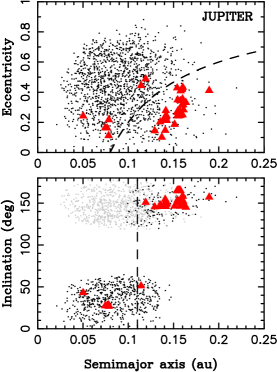
Figure 10: Left: Orbits of captured satellites (dots) and known irregular satellites at Jupiter (red triangles). The dashed line in the top panel denotes $q=a(1-e)=0.08$ au, which is an approximate limit below which the population of small retrograde satellites becomes strongly depleted by collisions with Himalia. The depleted orbits with $i>90^{\circ}$ and $q<0.08$ au are shown by gray dots in the bottom left panel. The dashed line in the bottom panel shows the boundary value $a=0.11$ au below which the collisions with Himalia should remove more than 50% of small retrograde satellites. Right: Orbits of irregular satellites at Saturn and Uranus. The results for Neptune, not shown here, can be found in NVM14.

To circumvent these problems, Nesvorný et al. (2007) suggested that the observed irregular satellites were captured from the heliocentric orbits during the time when fully-formed outer planets migrated in the planetesimal disk. They considered the original Nice model (Tsiganis et al. 2005). According to this model, Saturn and the ice giants repeatedly encounter each other before their orbits get stabilized. The encounters between planets remove any distant satellites that may have initially formed at Saturn, Uranus and Neptune by gas-assisted capture (or via a different mechanism). A new generation of satellites is then captured from the background planetesimal disk during planetary encounters. Capture happens when the trajectory of a background planetesimal is influenced in such a way by the approaching planets that the planetesimal ends up on a bound orbit around one of them, where it remains permanently trapped when planets move away from each other.

Modeling this mechanism in detail, Nesvorný et al. (2007) found that planetary encounters can create satellites on distant orbits at Saturn, Uranus and Neptune with orbital distributions that are broadly similar to those observed. Because Jupiter does not generally participate in planetary encounters in the original Nice model, however, the proposed mechanism was not expected to produce the irregular satellites at Jupiter. Things changed when the jumping-Jupiter model was proposed (Sections 4 and 5), because encounters of Jupiter with an ice giant planet is the defining feature of the jumping-Jupiter model. This offered an opportunity to develop a unified model where the irregular satellites of all outer planets are captured by the same mechanism (with similar capture efficiencies at each planet). This is desirable because the populations of irregular satellites at different planets are roughly similar (once it is accounted for the observational incompleteness; Jewitt & Sheppard 2005).

Nesvorný, Vokrouhlický & Morbidelli (2014a, hereafter NVM14) studied the capture of irregular satellites in the five-planet models from NM12 (Section 5). They found that the orbital distribution of bodies captured during planetary encounters provides a good match to the observed distribution of the irregular satellites at Jupiter, Saturn, Uranus and Neptune (Figure 10). The capture efficiency at Jupiter was found to be $(1.3$-$3.6)\times 10^{-8}$ for each planetesimal in the original outer disk. The calibration of the outer disk from Jupiter Trojans (Section 9) implies that there were $\simeq 6\times 10^{9}$ $D>10$ km planetesimals in the outer disk. Therefore, Jupiter’s encounters with the ejected ice giant should produce $\simeq 80$-220 $D>10$ km irregular satellites at Jupiter (NVM14). For comparison, only 10 $D>10$ km irregular satellites are known and this sample is thought to be complete.

The initially large population of captured satellites are expected to be reduced by disruptive collisions among satellites (Bottke et al. 2010). The results of the collisional cascade modeling imply a very shallow SFD slope for $D\sim 10$ km, exactly as observed. The satellite families provide a direct evidence for disruptive collisions of satellites (Nesvorný et al. 2003, Sheppard & Jewitt 2003). Collisions are also thought to be responsible for the observed asymmetry between the number of prograde (1 object) and retrograde (11 objects) irregular moons at Uranus. The asymmetry arises when the largest moon in the captured population eliminates smaller irregular moons that orbit the planet in the opposite sense (Bottke et al. 2010).

The regular moons of the outer planets also represent an important constraint on the history of planetary encounters. This is because the orbits of the regular moons can be perturbed by gravity of the passing planet. In an extreme case, when very deep encounters between planets occur, the orbits of regular moons could be excited and destabilized. Deienno et al. (2014) studied the effects of planetary encounters on the Galilean satellites in several migration/instability cases from NM12. They found that the strongest constraint on the encounters is derives from the small orbital inclinations of the Galilean moons ($i<1^{\circ}$). The inclinations of Galilean moons, if exited to $i>1^{\circ}$, would not evolve to $i<1^{\circ}$ by tidal damping over 4.5 Gyr. Thus, a strong excitation of inclinations during encounters must be avoided.

It has been determined that the largest orbital perturbations occur during a few deepest encounters (Deienno et al. 2014; the irregular satellites, instead, are captured by many encounters including the distant ones; NVM14). The simulation results imply that the encounters with the minimum distance $d<0.02$ au must avoided, and the encounters with $0.02<d<0.05$ au cannot be too many (for reference, Callisto has $a\simeq 0.012$ au). Roughly 50% of NM12 instability cases that satisfy the A-D criteria (Section 5) also satisfy this constraint. Interestingly, the distant encounters of Saturn with an ice giant could have excited the Iapetus’s inclination to its current value ($i\simeq 8^{\circ}$ with respect to the local Laplace plane) while leaving its eccentricity low (Nesvorný et al. 2014b).

The regular satellites of Uranus are a very sensitive probe of planetary encounters. This is because the most distant of these satellites, Oberon, has only $\simeq$0.068^∘ inclination with respect to the Laplace surface. Previous works done in the framework of the original Nice model and the jumping-Jupiter model with four planets (Deienno et al. 2011; Nogueira et al. 2013) had difficulties to satisfy this constraint, because Uranus experienced encounters with Jupiter and/or Saturn in these instability models. In the NM12 model, Uranus does not have encounters with Jupiter and Saturn, and instead experiences a small number of encounters with a relatively low-mass ice giant. Consequently, Oberon’s inclination remains below 0.1^∘ in nearly all cases taken from NM12. Neptune’s regular satellites are less of a constraint, because Triton’s orbit is closely bound to Neptune and has been strongly affected by tides (Correia et al. 2009).

11 KUIPER BELT

The Kuiper belt is a diverse population of bodies on trans-Neptunian orbits (Figure 11). Based on dynamical considerations, the Kuiper Belt Objects (KBOs) are classified (Gladman et al. 2008) into several groups: the resonant populations, classical belt, scattered/scattering disk, and detached objects (also known as the fossilized scattered disk). The resonant populations are a fascinating feature of the Kuiper belt. They give the Kuiper belt an appearance of a bar code with individual bars centered at the resonant orbital periods. Pluto and Plutinos in the 3:2 resonance with Neptune (orbital period $\simeq$250 yr) are the largest and best-characterized resonant group. The resonant bodies are long-lived, even if $q<Q_{\rm 8}$, where $Q_{\rm 8}=a_{8}(1-e_{8})\simeq 30.4$ au is the aphelion distance of Neptune, because they are phase-protected by resonances from close encounters with Neptune.

The orbits of the scattered/scattering disk objects (SDOs), on the other hand, evolved and keep evolving by close encounters with Neptune. These objects tend to have long orbital periods and be detected near their orbital perihelion when the heliocentric distance is $\sim$30 au. Their neighbors, the detached objects, have a slightly larger perihelion distance than the scattered/scattering objects and semimajor axes beyond the 2:1 resonance ($a>47.8$ au). The detached KBOs with very large semimajor axes ($a>150$ au) are sometimes referred to as the extreme SDOs. The observed orbital alignment of extreme SDOs has driven the recent interest in the Planet 9 hypothesis (Trujillo & Sheppard 2014, Batygin & Brown 2016).

The classical Kuiper Belt, hereafter CKB, is a population of trans-Neptunian bodies dynamically defined as having non-resonant orbits with perihelion distances that are large enough to avoid close encounters with Neptune. Most known KBOs reside in the main CKB located between the 3:2 and 2:1 resonances with Neptune ($39.4<a<47.8$ au). It is furthermore useful to divide the CKB into dynamically “cold” and “hot” components, mainly because the inclination distribution in the CKB is bimodal (Brown 2001, Gulbis et al. 2010), hinting at different dynamical origins of these groups. The Cold Classicals (CCs) are often defined as having $i<5^{\circ}$ and Hot Classicals (HCs) as $i>5^{\circ}$ (Figure 11). Note that this definition is somewhat arbitrary, because the continuous inclination distribution near $i=5^{\circ}$ indicates that significant mixing between the two components must have occurred (e.g., Volk & Malhotra 2011).

While HCs share many similarities with other dynamical classes of KBOs (e.g., scattered disk, Plutinos), CCs have several unique properties. Specifically, (1) CCs have distinctly red colors (e.g., Tegler & Romanishin 2000) that may have resulted from space weathering of surface ices, such as ammonia (e.g., Brown et al. 2011), that are stable beyond $\sim$35 au. (2) A large fraction of 100-km-class CCs are wide binaries with nearly equal size components (Noll et al. 2008). (3) The albedos of CCs are generally higher than those of HCs (Brucker et al. 2009). And finally, (4) the size distribution of CCs is markedly different from those of the hot and scattered populations, in that it shows a very steep slope at large sizes (e.g., Bernstein et al. 2004), and lacks very large objects. The most straightforward interpretation of these properties is that CCs formed and/or dynamically evolved by different processes than other trans-Neptunian populations.

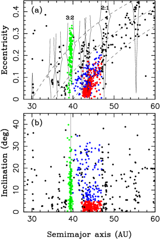
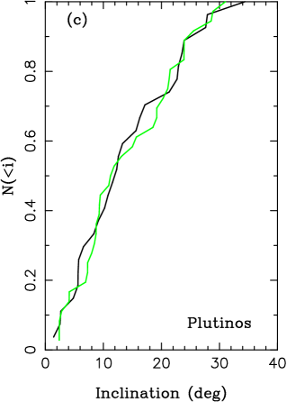
Figure 11: Left: Orbits of KBOs observed in three or more oppositions. Various dynamical classes are highlighted. HCs with $i>5^{\circ}$ are denoted by blue dots, and CCs with $i<5^{\circ}$ are denoted by red dots. The solid lines in panel (a) follow the borders of important orbital resonances. Note the wide inclination distribution of Plutinos (green dots) and HCs in panel (b) with inclinations reaching above $30^{\circ}$. Right: Comparison of the inclination distributions obtained in the model ($\tau=30$ Myr, $e_{8,0}=23$ au; Nesvorný & Vokrouhlický 2016; green line) and the Canada-France Ecliptic Plane Survey (CFEPS; Petit et al. 2011) detections (black line). The CFEPS detection simulator was applied to the model orbits to have a one-to-one comparison with the actual CFEPS detections.

The complex orbital structure of the trans-Neptunian region with heavily populated resonances, and high eccentricities and high inclinations of orbits (Figure 11), does not represent the dynamical conditions in which KBOs accreted. Instead, it is thought that much of this structure appeared as a result of Neptune’s migration. Following the pioneering work of Malhotra (1993, 1995), studies of Kuiper belt dynamics first considered the effects of outward migration of Neptune that can explain the prominent populations of KBOs in the major orbital resonances (Levison & Morbidelli 2003, Gomes 2003, Hahn & Malhotra 2005). With the advent of the notion that the early Solar System may have suffered a dynamical instability (Sections 3-5), the focus broadened, with recent theories invoking an eccentric and inclined orbit of Neptune (Levison et al. 2008, Batygin et al. 2011, Wolff et al. 2012, Dawson & Murray-Clay 2012, Morbidelli et al. 2014).

The emerging consensus is that HCs formed at $<$30 au, and were dynamically scattered to their current orbits by migrating/eccentric Neptune, while CCs formed at $>$40 au and survived Neptune’s early ‘wild days’ relatively unharmed. The main support for this model comes from the unique properties of CCs, which would be difficult to explain if HCs and CCs had similar formation locations (and dynamical histories). For example, the wide binaries observed among CCs would not survive scattering encounters with Neptune (Parker & Kavelaars 2010).

An outstanding problem with the previous models of Kuiper belt formation (e.g., Hahn & Malhotra 2005, Levison et al. 2008) is that the predicted distribution of orbital inclinations of Plutinos and HCs was found to be narrower than the one inferred from observations. The inclinations may have been excited before Neptune’s migration, but no such an early excitation process was identified so far. This problem appears to be more likely related to the timescale of Neptune’s migration. Nesvorný (2015a) performed numerical simulations of Kuiper belt formation starting from an initial state with a dynamically cold massive outer disk extending from beyond $a_{\rm N,0}$ to 30 au. According to arguments discussed in Sections 5, and the calibration from Jupiter Trojans (Section 9) the original disk mass was assumed to be $M_{\rm disk}\simeq 15$-20 $M_{\oplus}$.

In different simulations, Neptune was started with $20<a_{8,0}<30$ au and migrated into the disk on an e-folding timescale $1<\tau<100$ Myr to test the dependence of the results on the migration range and timescale. A small fraction of the disk planetesimals became implanted into the Kuiper belt in the simulations. To satisfy the inclination constraint (Figure 11c), it was found that Neptune’s migration must have been slow ($\tau\geq 10$ Myr) and long range ($a_{8,0}<25$ au). The models with $\tau<10$ Myr do not satisfy the inclination constraint, because there is not enough time for dynamical processes to raise inclinations. The slow migration of Neptune is consistent with other Kuiper belt constraints, and represents an important clue about the original mass of the outer disk. For example, in the NM12 planetary migration/instability model where the outer disk extends from $\simeq$23 to 30 au, $\tau\geq 10$ Myr implies $M_{\rm disk}\simeq 15$-20 $M_{\oplus}$.

Neptune’s eccentricity and inclination are never large in the NM12 models ($e_{\rm N}<0.15$, $i_{\rm N}<2^{\circ}$), as required to avoid excessive orbital excitation in the $>$40 au region, where the CCs formed. Simulations show that the CC population was dynamically depleted by only a factor of $\sim$2 (Nesvorný 2015b). This implies that the surface density of solids at 42-47 au was $\sim$4 orders of magnitude lower than the surface density needed to form sizable objects in the standard coagulation model (Kenyon et al. 2008). It is possible that the original surface density was higher and bodies were removed by fragmentation during collisions (Pan & Sari 2005), but the presence of loosely bound binaries places a strong constraint on how much mass can be removed by collisions (Nesvorný et al. 2011). Instead, these results suggest that CCs accreted in a low-mass environment (Youdin & Goodman 2005).

A particularly puzzling feature of the CC population is the so-called kernel, a concentration of orbits with $a=44$ au, $e\simeq 0.05$ and $i<5^{\circ}$ (Petit et al. 2011). This feature can either be interpreted as a sharp edge beyond which the number density of CCs drops, or as a genuine concentration of bodies. If it is the latter, the kernel can be explained if Neptune’s migration was interrupted by a discontinuous change of Neptune’s semimajor axis when Neptune reached $\simeq$27.7 au (the jumping-Neptune model; Petit et al. 2011, Nesvorný 2015b). Before the discontinuity happened, planetesimals located at $\sim$40 au were swept into the Neptune’s 2:1 resonance, and were carried with the migrating resonance outward (Levison & Morbidelli 2003). The 2:1 resonance was at $\simeq$44 au when Neptune reached $\simeq$27.7 au. If Neptune’s semimajor axis changed by a fraction of an au at this point, perhaps because it was scattered off of another planet (NM12), the 2:1 population would have been released at $\simeq$44 au, and would remain there to this day. The orbital distribution of bodies produced in this model provides a good match to the orbital properties of the kernel (Nesvorný 2015b).

Models with smooth migration of Neptune invariably predict excessively large resonant populations (e.g., Hahn & Malhotra 2005, Nesvorný 2015a), while observations show that the non-resonant orbits are in fact common (e.g., the classical belt population is $\simeq$2-4 times larger than Plutinos in the 3:2 resonance; Gladman et al. 2012). This problem can be resolved if Neptune’s migration was grainy, as expected from scattering encounters of Neptune with massive planetesimals. The grainy migration acts to destabilize resonant bodies with large libration amplitudes, a fraction of which ends up on stable non-resonant orbits. Thus, the non-resonant–to–resonant ratio obtained with the grainy migration is higher, up to $\sim$10 times higher for the range of parameters investigated in Nesvorný & Vokrouhlický (2016), than in a model with smooth migration. The best fit to observations was obtained when it was assumed that the outer planetesimal disk below 30 au contained 1000-4000 Plutos. The combined mass of Pluto-class objects in the original disk was thus $\sim$2-8 $M_{\oplus}$, which represents 10-50% of the estimated disk mass.

Together, the results discussed above imply that Neptune’s migration was slow, long-range and grainy, and that Neptune radially jumped by a fraction of an au when it reached 27.7 au. This is consistent with Neptune’s orbital evolution obtained in the NM12 models. Additional constraints on Neptune migration can be obtained from SDOs. Models imply that bodies scattered outward by Neptune to semimajor axes $a>50$ au often evolve into resonances which subsequently act to raise the perihelion distances of detached orbits to $q>40$ au (Gomes 2011). The implication of the model with slow migration of Neptune is that the orbits with $50<a<100$ au and $q>40$ au should cluster near (but not in) the resonances with Neptune (3:1 at $a=62.6$ au, 4:1 at $a=75.9$ au, 5:1 at $a=88.0$ au; Kaib & Sheppard 2016, Nesvorný et al. 2016). The recent detection of several distant KBOs near resonances is consistent with this prediction, but it is not yet clear whether most orbits are really non-resonant.

12 COMETARY RESERVOIRS

Comets are icy objects that reach the inner Solar System after leaving distant reservoirs beyond Neptune and dynamically evolving onto elongated orbits with very low perihelion distances (Dones et al. 2015). Their activity, manifesting itself by the presence of a dust/gas coma and characteristic tail, is driven by solar heating and sublimation of water ice. Comets are short-lived, implying that they must be resupplied from external reservoirs (Fernández 1980, Duncan et al. 1988).

Levison & Duncan (1997, hereafter LD97) considered the origin and evolution of ecliptic comets (ECs; see Figure 12 for their relationship to the Jupiter-family comets, JFCs). The Kuiper belt at 30-50 au was assumed in LD97 to be the main source reservoir of ECs. Small KBOs evolving onto a Neptune-crossing orbit can be slingshot, by encounters with different planets, to very low perihelion distances ($q<2.5$ au), at which point they are expected to become active and visible. The new ECs, reaching $q<2.5$ au for the first time, have a narrow inclination distribution in the LD97 model, because their orbits were assumed to start with low inclinations ($i<5^{\circ}$) in the Kuiper belt, and the inclinations stay low during the orbital transfer.

The escape of bodies from the classical KB at 30-50 au is driven by slow chaotic processes in various orbital resonances with Neptune. Because these processes affect only part of the belt, with most orbits in the belt being stable, questions arise about the overall efficiency of comet delivery from the classical KB. Duncan & Levison (1997), concurrently with the discovery of the first SDO; (15874) 1996 TL66, Luu et al. 1997), suggested that the scattered disk should be a more prolific source of ECs than the classical KB. This is because SDOs can always approach Neptune during their perihelion passages and be scattered by Neptune to orbits with shorter orbital periods.

The Halley-type comets (HTCs) have longer orbital periods and larger inclinations than do most ECs. It has been suggested that HTCs evolve into the inner Solar System from an inner, presumably flattened part of the Oort cloud (Levison et al. 2001). This theory was motivated by the inclination distribution of HTCs, which was thought to be flattened with a median of $\simeq$45^∘. Later on, the scattered disk was considered as the main source of HTCs (Levison et al. 2006). Back in 2006, the median orbital inclination of HTCs was thought to be $\simeq$55^∘, somewhat larger than in 2001, but still clearly anisotropic. This turns out to be part of a historical trend with the presently available data indicating a nearly isotropic inclination distribution of HTC orbits (Wang & Brasser 2014).

The ECs/JFCs and HTCs are also known as the Short-Period Comets (SPCs), defined as bodies showing cometary activity and having short orbital periods ($P<200$ yr). The period range is arbitrary, because there is nothing special about the boundary at the 200-yr period, and the orbital period distribution of known comets appears to continue smoothly across this boundary. With $P<200$ yr, SPCs are guaranteed to have at least one perihelion passage in modern history, with many being observed multiple times. This contrasts with the situation for the Long-Period Comets (LPCs; $P>200$ yr), which can be detected only if their perihelion passage coincides with the present epoch. Disregarding the period cutoff, HTCs and LPCs have the common property of having the Tisserand parameter with respect to Jupiter $T_{\rm J}<2$, and are referred to as the Nearly Isotropic Comets (NICs; LD97 and Figure 12). The main reservoir of LPCs is thought to be the Oort cloud, a roughly spherical structure of bodies at orbital distances $\simeq$$10^{4}$-$10^{5}$ au from the Sun.

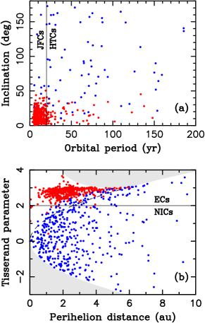
Figure 12: Left: The orbital distribution of known SPCs. The thin lines show the division between JFCs and HTCs (panel a; $P=20$ yr), and between ECs and NICs (panel b; Tisserand parameter $T_{\rm J}=2$). The color indicates the relationship between different categories. In panel a, the red dots denote ECs with $T_{\rm J}>2$, and the blue dots denote NICs with $T_{\rm J}<2$. In panel b, the red dots denote JFCs with $P<20$ yr, and the blue dots denote comets with $P>20$ yr and $a<10,$000 au. The gray areas in panel b cannot be reached by orbits. The dashed line in panel b is $T_{\rm J}=2\sqrt{2q}$, which is an approximate boundary of prograde orbits evolving from $a\gg a_{\rm J}$ and $e\sim 1$. Right: The cumulative orbital distributions of ECs with $P<20$ yr, $2<T_{\rm J}<3$ and $q<2.5$ au. The model results (solid lines; N17) are compared to the distribution of known JFCs (dashed lines). In the model, it was assumed that ECs remain active and visible for $N_{\rm p}(2.5)=500$ perihelion passages with $q<2.5$ au.

Our understanding of the origin and evolution of comets is incomplete in part because the presumed source populations of trans-Neptunian objects with cometary sizes ($\sim$1-10 km) are not well characterized from observations. It is therefore difficult to establish whether there are enough small objects in any trans-Neptunian reservoir to provide the source of comets (e.g., Volk & Malhotra 2008). To circumvent this problem, several recently developed models performed end-to-end simulations in which cometary reservoirs are produced in the early Solar System and evolved over 4.5 Gyr (Brasser & Morbidelli 2013; Nesvorný et al. 2017a, hereafter N17). The number of comets produced in the model at the present time can then be inferred from the number of comets in the original planetesimal disk, which in turn can be calibrated from the number of Jupiter Trojans (Section 9; Figure 9).

This approach, to be reliable, requires that we have a good model for the early evolution of the Solar System, which was adopted from NM12 (Section 5). The steady state model of ECs/JFCs obtained in the NM12 model can be compared to observations. To do this comparison correctly, as pointed out in LD97, it must be accounted for the physical lifetime of active comets (i.e., how long comets remain active). Several different parametrizations of the physical lifetime were considered in N17. In the simplest parametrization, they counted the number of perihelion passages with $q<2.5$ au, $N_{\rm p}(2.5)$, and assumed that a comet becomes inactive if $N_{\rm p}(2.5)$ exceeds some threshold. The threshold was determined by the orbital fits to observations.

The orbital distribution of ECs was well reproduced in the model (Figure 12). The nominal fit to the observed inclination distribution of JFCs requires, on average, that km-sized JFCs survive $N_{\rm p}(2.5)\simeq 500$ perihelion passages with $q<2.5$ au. This is consistent with the measured mass loss of 67P/Churyumov-Gerasimenko (Paetzold et al. 2016). To explain the number of known large ECs ($D>10$ km), large comets are required to have longer physical lifetimes than small comets. The dependence of $N_{\rm p}(2.5)$ on comet size for $D<1$ km is poorly constrained, but the physical lifetime should drop more steeply than a simple extrapolation from $D>1$ km to $D<1$ km would suggest. This is because $N_{\rm p}(2.5)<10$ is required to match the ratio of returning-to-new LPCs, which presumably have $D<1$ km (Brasser & Morbidelli 2013). The hypothesized transition to very short physical lifetimes for comets below 1 km may be related to the rotational spin-up of small cometary nuclei and their subsequent disruption by the centrifugal force.

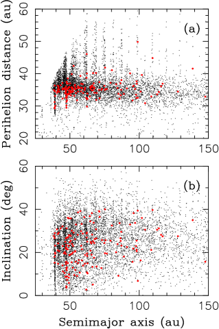
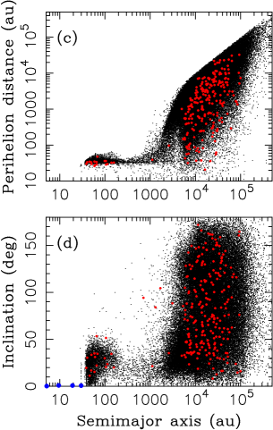
Figure 13: The orbits of trans-Neptunian bodies that dynamically evolve to become SPCs. The source of ECs is shown on the left (panels a and b). The source of HTCs is shown on the right (panels c and d). ECs were selected using $2<T_{\rm J}<3$, $P<20$ yr and $q<2.5$ au and $N_{\rm p}(2.5)=500$. The source orbits of ECs were identified at $t=1.5$ Gyr after $t_{0}$ (i.e., about 3 Gyr ago), and plotted here with red dots. HTCs were selected using $T_{\rm J}<2$, $10<a<20$ au and $q<2$ au and $N_{\rm p}(2.5)=3000$. The source orbits of HTCs are plotted at $t=3.5$ Gyr or about 1 Gyr ago. Background orbits are denoted by black dots.

The source reservoir of most ECs ($\simeq$75%) is the scattered disk with $50<a<200$ au (Figure 13). About 20% of ECs started with $a<50$ au. The classical KB, including various resonant populations below 50 au (about 4% of ECs evolved from the Plutino population), is therefore a relatively important source of ECs. Interestingly, $\simeq$3% of model ECs started in the Oort cloud. The orbital evolution of these comets is similar to returning LPCs or HTCs, except that they were able to reach orbits with very low orbital periods and low inclinations. The median semimajor axis of source EC orbits is $\simeq$60 au.

HTCs were found to have a nearly isotropic inclination distribution and appear as an extension of the population of returning LPCs to shorter orbital periods (N17). The number of large HTCs obtained in the model from the Oort cloud agrees well with observations. A great majority ($\simeq$95%) of HTCs come from the Oort cloud, and only $\simeq$5% from the $a<100$ au region (Figure 13). The inclination distribution of source orbits in the Oort cloud is slightly anisotropic with the median inclination $\simeq$$70^{\circ}$. This is similar to the median inclination of new HTCs in the N17 model. The inner and outer parts of the Oort cloud (1,$000<a<20,$000 au inner, $a>20,$000 au outer), contribute in nearly equal proportions to the HTC population.

The inner scattered disk at $50<a<200$ au should contain $\sim 1.5\times 10^{7}$ $D>10$ km bodies, and the Oort cloud should contain $\sim 3.8\times 10^{8}$ $D>10$ km comets. These estimates were obtained by calibrating the original outer disk from Jupiter Trojans (Section 9) and propagating all populations to the current epoch. They are consistent with the number of observed comets that evolve from these reservoirs to the inner Solar System (see also Brasser & Morbidelli 2013). The above estimates can be extrapolated to smaller or larger sizes using the size distribution of Jupiter Trojans (Figure 9).

13 LATE HEAVY BOMBARDMENT

The impact cratering record of the Moon and the terrestrial planets provides important clues about the formation and evolution of the Solar System (Bottke et al. 2017). Especially intriguing is the epoch $\simeq$3.8-3.9 Gyr ago (Ga), known as the Late Heavy Bombardment (LHB), when the youngest lunar basins such as Imbrium and Orientale formed (see Chapman et al. 2007 for a review). It has been argued that the impact record can be best understood as a ‘sawtooth’ profile (Bottke et al. 2012, Morbidelli et al. 2012b, Marchi et al. 2012), a combination of decaying flux from the terrestrial planet accretion leftovers, and a modest increase in the number of asteroid/comet impacts (by a factor of 5 or so) produced by a dynamical instability in the outer Solar System (Section 3). These works assumed that the instability happened late, some $\simeq$3.8-4.2 Ga or $\sim$400-700 Myr after $t_{0}$.

The time of planetary migration/instability cannot be determined from the modeling alone, because it depends on unknown details of the Solar System architecture at the time of the gas disk dispersal. The late version of the instability/migration was advocated by the proponents of its relation to the LHB (see the references above). It could also explain the shock age distribution of various meteorite classes which show a period of enhanced collisional activity around the LHB time. The instability could have been delayed if the inner edge of the outer planetesimal disk was well separated, by a few au, from the outermost planet, such that it took a while for planetesimals to reach the planet-crossing orbits (Gomes et al. 2005). It could have been triggered by distant perturbations from the outer disk planetesimals (Levison et al. 2011) or by interaction of planets with large amounts of dust evolving inward from the outer disk by Poynting-Robertson drag (Deienno et al. 2017).

The early instability, on the other hand, offers several notable advantages. First, the instabilities in dynamical systems generally happen early, not late. To trigger a late instability in the outer Solar System, and obtain planetary evolution histories that are compatible with the observed structure of the Kuiper belt, the parameters of the outer planetesimal disk may need to be fine tuned (Gomes et al. 2005, Deienno et al. 2017). Second, the early version of the dynamical instability would relax the terrestrial planet constraint (Agnor & Lin 2012, Kaib & Chambers 2016), because the secular resonances would sweep through the inner Solar System before the terrestrial system was in place (Section 7). Third, the analyses of Highly Siderophile Elements (HSEs; Kring & Cohen 2002) and oxygen isotopes (Joy et al. 2012) do not provide any firm evidence for cometary impactors, while dynamical models indicate that the number of cometary impacts during the instability should have dwarfed the asteroid impacts. There is no problem with the cometary impactors if the instability happened early, because the early impacts would not be recorded in the geochemical markers.

A recent study of impacts on the terrestrial worlds was reported in Nesvorný, Roig & Bottke (2017; hereafter NRB17). NRB17 developed a dynamical model for the historical flux of large asteroid and comet impactors and discussed how it depends on various parameters, including the time and nature of the planetary migration/instability. The orbital evolution of planets in different cases was taken from Bottke et al. (2012), NM12 and Roig et al. (2016). They found that the asteroid impact flux dropped by 1 to 2 orders of magnitude during the first 1 Gyr and remained relatively unchanged over the last 3 Gyr. The early impacts were produced by asteroids whose orbits became excited during the planetary migration/instability, and by those originating from the inner extension of the main belt (E-belt; semimajor axis $1.6<a<2.1$ au, Bottke et al. 2012).

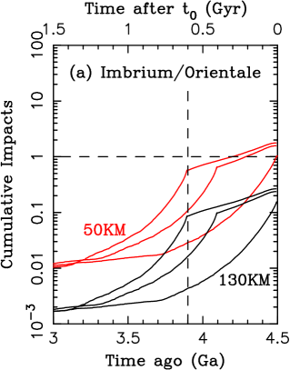
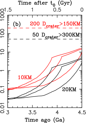
Figure 14: A comparison of constraints from large lunar craters and basins with the asteroid impact fluxes from NRB17. Panel (a) highlights the constraint from the Orientale and Imbrium basins. The family of solid black curves shows the calibrated impact profile of $D=130$-km (Imbrium) impactors for three different values of the instability time ($t_{\rm inst}=3.9$, 4.1 and 4.5 Ga). The red curves show the same for the $D=50$-km (Orientale) impactors. Panel (b) reports the results of dynamical modeling relevant for the $D>150$-km lunar craters and $D>300$-km lunar basins, here assumed to require $D>10$ km and $D>20$ km asteroid impacts at 23 km s^-1. The red dashed line in (b) shows the number of $D>150$-km lunar craters, obtained by scaling the crater densities from the heavily cratered, ancient terrains on the far side of the Moon to the whole lunar surface (Bottke et al. 2017). In total, only $\sim$10-15 $D>10$-km asteroids should have impacted the Moon, with all these impacts happening during the first 1 Gyr of the Solar System history. The Earth and Venus received $\sim$20 times as many, or $\sim$200-300 $D>10$ km asteroid impactors.

The asteroid impact flux was absolutely calibrated in NRB17. To this end, the number of bodies surviving in the asteroid belt at $t=4.5$ Gyr after the start of the integration was compared with the actual number of known main belt asteroids of given size (for example, there are $\simeq$8000 asteroids with $D>10$ km; Masiero et al. 2014). This resulted in a factor that was applied to compute an absolutely calibrated historical record of impacts. The results indicate that asteroids were probably not responsible for the LHB, independently of whether the instability happened early or late, because the calibrated flux is not large enough to explain Imbrium/Orientale and a significant share of large lunar craters (Figure 14).

Comets (Levison et al. 2001, Gomes et al. 2005) and leftovers of the terrestrial planet accretion (Morbidelli et al. 2001, 2017) provided additional, and perhaps dominant source of impacts. The number of comets in the original outer disk can be absolutely calibrated from Jupiter Trojans. The cometary impact flux on the terrestrial worlds can then be estimated from dynamical integrations (Gomes et al. 2005, NRB17). The results show that the overall impact probabilities of comets on the Earth are $\simeq 5\times 10^{-7}$ (for each comet in the original disk). With $\simeq 6\times 10^{9}$ $D>10$ km comets in the original disk (Figure 9), this implies $\sim$3000 terrestrial impacts of $D>10$ km comets. This is $\sim$10-15 times the expected number of asteroid impacts. The Moon should have received $\sim$1/20 of the terrestrial flux, or $\sim$150 $D>10$ km comet impactors. Since the geochemical evidence argues against comets being the main source of the LHB, this may indicate that the instability happened early (i.e., before the lunar surface was able to record large impacts).

New terrestrial planet formation models show that that leftover impact flux probably decayed more slowly (Morbidelli et al. 2017) than thought before (Bottke et al. 2007). Unfortunately, the terrestrial planet formation is still not understood well enough to absolutely calibrate the leftover impact flux. Instead, possible impact histories can be obtained from various geochemical constraints. For example, assuming that the HSEs track the total amount of material accreted by the Moon since its formation would imply that the LHB was a spike in the bombardment flux (Morbidelli et al. 2012b). If the HSEs were depleted from Moon’s mantle during magma ocean crystallization, due to iron sulfide exsolution (Rubie et al. 2016), however, the LHB can be explained as tail of slowly decaying impact flux of the terrestrial planet leftovers (Morbidelli et al. 2017). This would imply that the lunar magma ocean crystallized $\sim$100 Myr after the Moon’s formation.

14 SUMMARY

Historically, it was thought that the planets formed near their current locations. However, starting with the pioneering works of Goldreich and Tremaine (for planet–gas disk interactions) in the late 1970s and Fernández and Ip (for planet–planetesimal disk interactions) in the early 1980s, it has become clear that the structure of the outer Solar System, at least, most likely changed as the planets grew and migrated. As we have broadened our horizons concerning the theory of planet formation, we have significantly increased the size of the parameter space that we need to explore. As a result, we have gotten to the point where we need to use any available constraint on the problem.

In sections 6-13, we discussed various constraints on the dynamical evolution of the early Solar System.

Section 6: The obliquities of the giant planets constrain the behavior of the $s_{7}$ and $s_{8}$ frequencies that govern the orbital plane precession of Uranus and Neptune. The frequency $s_{8}$ is required to evolve fast initially and very slowly toward the end of planetary migration. This happens in most migration models as Neptune’s migration tends to slow down over time. At late stages, the effective e-folding migration timescale must have been $100<\tau<200$ Myr for Saturn’s obliquity to be excited by capture in the spin-orbit resonance with $s_{8}$.

Section 7: The terrestrial planets are a very sensitive probe of the behavior of the $g_{5}$ frequency that controls the precession of Jupiter’s orbit. If the instability happened late, when the terrestrial planet system was already in place, the resonances of $g_{1}$ (Mercury) and $g_{2}$ (Venus) with $g_{5}$ must be avoided, because they would lead to an excessive orbital excitation of the terrestrial planets. This can be best accomplished in the jumping-Jupiter model where the $g_{5}$ frequency has a discontinuity as a result of planetary encounters.

Section 8: The asteroid belt constraints suggest that the $g_{6}$ (precession of Saturn’s orbit) and $s_{6}$ (precession Saturn’s orbital plane) frequencies changed fast such that the $s=s_{6}$ and $g=g_{6}$ resonances spent much less than 1 Myr in the 2-3 au region. This happens in the jumping-Jupiter model, where the period ratio $P_{6}/P_{5}$ changes from $<$2 to $>$2.3 in $\ll$1 Myr, and the resonances only briefly overlap with the inner part of the asteroid belt ($a<2.5$ au). The asteroid constraint applies independently of whether the instability happened early or late.

Section 9: From modeling the planetary migration/instability, NM12 estimated that the mass of the outer disk of planetesimals (23-30 au) was $M_{\rm disk}\simeq 15$-20 $M_{\oplus}$. An independent estimate of $M_{\rm disk}$ can be obtained from the capture probability and present population of Jupiter Trojans. This estimate also gives $M_{\rm disk}\simeq 15$-20 $M_{\oplus}$, providing support for the NM12 model.

Section 10: The moons of the giant planets represent important constraints on planetary encounters during the instability. The orbital inclinations of Uranus’s regular moons suggest that Uranus probably did not have close encounters with Jupiter/Saturn. The Galilean moons at Jupiter imply that there were no encounters between Jupiter and an ice giant with mutual distance $d<0.02$ au. The similar populations of irregular satellites at different planets suggest that all giant planets had at least several distant encounters with another planet.

Section 11: The Kuiper belt constraints imply that Neptune’s migration was slow ($\tau\geq 10$ Myr), long range ($a_{8,0}\leq 25$ au) and grainy (1000-4000 Pluto-class objects in the original outer disk). The migration timescale implies that the outer disk at 23-30 au had mass $M_{\rm disk}\simeq 15$-20 $M_{\oplus}$, which is consistent with several independent estimates discussed above. Encounters of Neptune with the fifth planet, which produce a discontinuity during Neptune’s migration, can explain the Kuiper belt kernel.

Section 12: Modeling implies that the inner scattered disk at $50<a<200$ au should contain $\sim 1.5\times 10^{7}$ $D>10$ km bodies. The Oort cloud should contain $\sim 3.8\times 10^{8}$ $D>10$ km comets. The number of large JFCs and HTCs obtained from these reservoirs in the model is consistent with the number of observed comets. To fit various constraints, the physical lifetime of comets must be a strong function of comet size.

Section 13: The absolute calibration of the impact flux indicates that asteroids were probably not responsible for the LHB, independently of whether the instability happened early or late, because the calibrated flux is not large enough to explain Imbrium/Orientale and a significant proportion of large lunar craters. Therefore, attempts to delay the instability may not be useful. Comets and leftovers of the terrestrial planet accretion probably provided a dominant source of impacts on the terrestrial worlds during early epochs.

Although significant uncertainties remain, the Solar System constraints discussed above allow us piece together the following sequence of events in the early Solar System history. The outer planets emerged from the protoplanetary gas disk in a compact resonant configuration with Jupiter and Saturn in the 3:2 (or 2:1) resonance and Neptune at $\simeq 20$-25 au. The third ice giant planet with the mass similar to Uranus or Neptune was located near $\simeq 10$ au (between the original orbits of Saturn and Uranus). The outer planetesimal disk extended from just outside of Neptune’s orbit to $\simeq$30 au, and had a low mass extension reaching to at least $\simeq$47 au. Several independent estimates suggest $M_{\rm disk}\simeq 15$-20 $M_{\oplus}$ and the SFD of the disk planetesimals similar to that of present-day Jupiter Trojans.

Within a few tens of Myr, Neptune slowly migrated into the planetesimal disk, scattering planetesimals around, and taking $>$10 Myr to reach its current orbit near 30 au. The other planets migrated as well. During the planetary migration, probably when Neptune reached $\simeq$27.7 au, a dynamical instability occurred with the fifth planet having encounters with all other outer planets. It was subsequently ejected from the Solar System by Jupiter. As a result, Jupiter’s semimajor axis changed by a fraction of an au and Jupiter’s proper eccentricity mode was excited to its current value. The inner part of the asteroid belt was destabilized by resonances with Jupiter and contributed to the early impacts in the inner Solar System. If the terrestrial planet formation was not completed at this point, these early impacts would not be recorded on surfaces of the terrestrial worlds. Mercury’s orbit may have been excited during the instability.

In the end, the outer planetesimal disk was completely dispersed by planets and parts of it were implanted into different populations, including the asteroid belt (estimated implantation probability $5\times 10^{-6}$), Jupiter Trojans ($5\times 10^{-7}$), Jupiter irregular satellites ($2.5\times 10^{-8}$), Kuiper belt ($10^{-3}$), scattered disk ($3\times 10^{-3}$), and the Oort cloud ($5\times 10^{-2}$). The size and orbital distributions of bodies in these populations, either observed or inferred indirectly, are consistent with the planetary migration/instability model discussed above. In fact, as we argued throughout this text, the populations of small bodies in the Solar System represent fundamental constraints on the early dynamical evolution of the Solar System. The model of planetary migration/instability outlined above was developed in an attempt to satisfy them all.

15 DISCLOSURE STATEMENT

The authors are not aware of any affiliations, memberships, funding, or financial holdings that might be perceived as affecting the objectivity of this review.

16 ACKNOWLEDGMENTS

This work was was sponsored by the NASA Emerging Worlds program. Luke Dones, Alessandro Morbidelli and David Vokrouhlický supplied many helpful comments to the manuscript. I dedicate this text to my father Jan.

References

- [Adams(2010)] Adams, F. C. 2010. Annual Review of Astronomy and Astrophysics 48: 47–85
- [Adams et al.(2014)] Adams, E. R., Gulbis, A. A. S., Elliot, J. L., et al. 2014. The Astronomical Journal 148: 55–
- [Agnor & Hamilton(2006)] Agnor, C. B., & Hamilton, D. P. 2006. Nature 441: 192–194
- [Agnor & Lin(2012)] Agnor, C. B., & Lin, D. N. C. 2012. The Astrophysical Journal 745: 143–
- [Asphaug & Reufer(2014)] Asphaug, E., & Reufer, A. 2014. Nature Geoscience 7: 564–568
- [Batygin & Brown(2016)] Batygin, K., & Brown, M. E. 2016. The Astronomical Journal 151: 22–
- [Batygin, Brown, & Fraser(2011)] Batygin, K., Brown, M. E., & Fraser, W. C. 2011. The Astrophysical Journal 738: 13–
- [Batygin, Brown, & Betts(2012)] Batygin, K., Brown, M. E., & Betts, H. 2012. The Astrophysical Journal 744: L3–
- [Beaugé, Roig, & Nesvorný(2002)] Beaugé, C., Roig, F., & Nesvorný, D. 2002. Icarus 158: 483–498
- [Bernstein et al.(2004)] Bernstein, G. M., Trilling, D. E., Allen, R. L., et al. 2004. The Astronomical Journal 128: 1364–1390
- [Bottke, Levison, Nesvorný, & Dones(2007)] Bottke, W. F., Levison, H. F., Nesvorný, D., & Dones, L. 2007. Icarus 190: 203–223
- [Bottke, Nesvorný, Vokrouhlický, & Morbidelli(2010)] Bottke, W. F., Nesvorný, D., Vokrouhlický, D., & Morbidelli, A. 2010. The Astronomical Journal 139: 994–1014
- [Bottke et al.(2012)] Bottke, W. F., Vokrouhlický, D., Minton, D., et al. 2012. Nature 485: 78–81
- [Boué, Laskar, & Kuchynka(2009)] Boué, G., Laskar, J., & Kuchynka, P. 2009. The Astrophysical Journal 702: L19–L22
- [Brasil et al.(2016)] Brasil, P. I. O., Roig, F., Nesvorný, D., et al. 2016. Icarus 266: 142–151
- [Brasser & Morbidelli(2013)] Brasser, R., & Morbidelli, A. 2013. Icarus 225: 40–49
- [Brasser & Lee(2015)] Brasser, R., & Lee, M. H. 2015. The Astronomical Journal 150: 157–
- [Brasser et al.(2009)] Brasser, R., Morbidelli, A., Gomes, R., Tsiganis, K., & Levison, H. F. 2009. Astronomy and Astrophysics 507: 1053–1065
- [Brasser, Walsh, & Nesvorný(2013)] Brasser, R., Walsh, K. J., & Nesvorný, D. 2013. Monthly Notices of the Royal Astronomical Society 433: 3417–3427
- [Brown(2001)] Brown, M. E. 2001. The Astronomical Journal 121: 2804–2814
- [Brown, Schaller, & Fraser(2011)] Brown, M. E., Schaller, E. L., & Fraser, W. C. 2011. The Astrophysical Journal 739: L60–
- [Brucker et al.(2009)] Brucker, M. J., Grundy, W. M., Stansberry, J. A., et al. 2009. Icarus 201: 284–294
- [Buie et al.(2015)] Buie, M. W., Olkin, C. B., Merline, W. J., et al. 2015. The Astronomical Journal 149: 113–
- [Chapman, Cohen, & Grinspoon(2007)] Chapman, C. R., Cohen, B. A., & Grinspoon, D. H. 2007. Icarus 189: 233–245
- [Charnoz, Salmon, & Crida(2010)] Charnoz, S., Salmon, J., & Crida, A. 2010. Nature 465: 752–754
- [Correia(2009)] Correia, A. C. M. 2009. The Astrophysical Journal 704: L1–L4
- [Cuk(2007)] Cuk, M. 2007. Bulletin of the American Astronomical Society 39: 60.05–
- [Ćuk & Burns(2004)] Ćuk, M., & Burns, J. A. 2004. Icarus 167: 369–381
- [Dawson & Murray-Clay(2012)] Dawson, R. I., & Murray-Clay, R. 2012. The Astrophysical Journal 750: 43–
- [Deienno et al.(2011)] Deienno, R., Yokoyama, T., Nogueira, E. C., Callegari, N., & Santos, M. T. 2011. Astronomy and Astrophysics 536: A57–
- [Deienno, Nesvorný, Vokrouhlický, & Yokoyama(2014)] Deienno, R., Nesvorný, D., Vokrouhlický, D., & Yokoyama, T. 2014. The Astronomical Journal 148: 25–
- [Deienno et al.(2016)] Deienno, R., Gomes, R. S., Walsh, K. J., Morbidelli, A., & Nesvorný, D. 2016. Icarus 272: 114–124
- [Deienno, Morbidelli, Gomes, & Nesvorný(2017)] Deienno, R., Morbidelli, A., Gomes, R. S., & Nesvorný, D. 2017. The Astronomical Journal 153: 153–
- [DeMeo et al.(2015)] DeMeo, F. E., Alexander, C. M. O., Walsh, K. J., Chapman, C. R., & Binzel, R. P. 2015. Asteroids IV 13–41
- [Dones, Brasser, Kaib, & Rickman(2015)] Dones, L., Brasser, R., Kaib, N., & Rickman, H. 2015. Space Science Reviews 197: 191–269
- [Duncan & Levison(1997)] Duncan, M. J., & Levison, H. F. 1997. Science 276: 1670–1672
- [Duncan, Quinn, & Tremaine(1988)] Duncan, M., Quinn, T., & Tremaine, S. 1988. The Astrophysical Journal 328: L69–L73
- [Fernandez(1980)] Fernd́ez, J. A. 1980. Icarus 42: 406–421
- [Fernandez & Ip(1984)] Fernd́ez, J. A., & Ip, W.-H. 1984. Icarus 58: 109–120
- [Ford & Chiang(2007)] Ford, E. B., & Chiang, E. I. 2007. The Astrophysical Journal 661: 602–615
- [Fraser et al.(2014)] Fraser, W. C., Brown, M. E., Morbidelli, A., Parker, A., & Batygin, K. 2014. The Astrophysical Journal 782: 100–
- [Gladman, Marsden, & Vanlaerhoven(2008)] Gladman, B., Marsden, B. G., & Vanlaerhoven, C. 2008. The Solar System Beyond Neptune 43–57
- [Gladman et al.(2012)] Gladman, B., Lawler, S. M., Petit, J.-M., et al. 2012. The Astronomical Journal 144: 23–
- [Gomes(2003)] Gomes, R. S. 2003. Icarus 161: 404–418
- [Gomes(2011)] Gomes, R. S. 2011. Icarus 215: 661–668
- [Gomes, Morbidelli, & Levison(2004)] Gomes, R. S., Morbidelli, A., & Levison, H. F. 2004. Icarus 170: 492–507
- [Gomes, Levison, Tsiganis, & Morbidelli(2005)] Gomes, R., Levison, H. F., Tsiganis, K., & Morbidelli, A. 2005. Nature 435: 466–469
- [Gradie & Tedesco(1982)] Gradie, J., & Tedesco, E. 1982. Science 216: 1405–1407
- [Grav et al.(2011)] Grav, T., Mainzer, A. K., Bauer, J., et al. 2011. The Astrophysical Journal 742: 40–
- [Gulbis et al.(2010)] Gulbis, A. A. S., Elliot, J. L., Adams, E. R., et al. 2010. The Astronomical Journal 140: 350–369
- [Hahn & Malhotra(1999)] Hahn, J. M., & Malhotra, R. 1999. The Astronomical Journal 117: 3041–3053
- [Hahn & Malhotra(2005)] Hahn, J. M., & Malhotra, R. 2005. The Astronomical Journal 130: 2392–2414
- [Hamilton & Ward(2004)] Hamilton, D. P., & Ward, W. R. 2004. The Astronomical Journal 128: 2510–2517
- [Hayashi(1981)] Hayashi, C. 1981. Progress of Theoretical Physics Supplement 70: 35–53
- [Helled, Schubert, & Anderson(2009)] Helled, R., Schubert, G., & Anderson, J. D. 2009. Icarus 199: 368–377
- [Helled, Anderson, Schubert, & Stevenson(2011)] Helled, R., Anderson, J. D., Schubert, G., & Stevenson, D. J. 2011. Icarus 216: 440–448
- [Izidoro et al.(2015)] Izidoro, A., Morbidelli, A., Raymond, S. N., Hersant, F., & Pierens, A. 2015. Astronomy and Astrophysics 582: A99–
- [Jacobson et al.(2014)] Jacobson, S. A., Morbidelli, A., Raymond, S. N., et al. 2014. Nature 508: 84–87
- [Jewitt & Sheppard(2005)] Jewitt, D., & Sheppard, S. 2005. Space Science Reviews 116: 441–455
- [Joy et al.(2012)] Joy, K. H., Zolensky, M. E., Nagashima, K., et al. 2012. Science 336: 1426–
- [Kaib & Chambers(2016)] Kaib, N. A., & Chambers, J. E. 2016. Monthly Notices of the Royal Astronomical Society 455: 3561–3569
- [Kaib & Sheppard(2016)] Kaib, N. A., & Sheppard, S. S. 2016. The Astronomical Journal 152: 133–
- [Kenyon, Bromley, O’Brien, & Davis(2008)] Kenyon, S. J., Bromley, B. C., O’Brien, D. P., & Davis, D. R. 2008. The Solar System Beyond Neptune 293–313
- [Kleine et al.(2009)] Kleine, T., Touboul, M., Bourdon, B., et al. 2009. Geochimica et Cosmochimica Acta 73: 5150–5188
- [Kley & Nelson(2012)] Kley, W., & Nelson, R. P. 2012. Annual Review of Astronomy and Astrophysics 50: 211–249
- [Kring & Cohen(2002)] Kring, D. A., & Cohen, B. A. 2002. Journal of Geophysical Research (Planets) 107: 5009–1
- [Kruijer, Burkhardt, Budde, & Kleine(2017)] Kruijer, T. S., Burkhardt, C., Budde, G., & Kleine, T. 2017. Proceedings of the National Academy of Science 114: 6712–6716
- [Laskar(1996)] Laskar, J. 1996. Celestial Mechanics and Dynamical Astronomy 64: 115–162
- [Levison & Duncan(1997)] Levison, H. F., & Duncan, M. J. 1997. Icarus 127: 13–32
- [Levison & Morbidelli(2003)] Levison, H. F., & Morbidelli, A. 2003. Nature 426: 419–421
- [Levison et al.(2001)] Levison, H. F., Dones, L., Chapman, C. R., et al. 2001. Icarus 151: 286–306
- [Levison, Dones, & Duncan(2001)] Levison, H. F., Dones, L., & Duncan, M. J. 2001. The Astronomical Journal 121: 2253–2267
- [Levison, Duncan, Dones, & Gladman(2006)] Levison, H. F., Duncan, M. J., Dones, L., & Gladman, B. J. 2006. Icarus 184: 619–633
- [Levison et al.(2008)] Levison, H. F., Morbidelli, A., Van Laerhoven, C., Gomes, R., & Tsiganis, K. 2008. Icarus 196: 258–273
- [Levison et al.(2009)] Levison, H. F., Bottke, W. F., Gounelle, M., et al. 2009. Nature 460: 364–366
- [Levison et al.(2011)] Levison, H. F., Morbidelli, A., Tsiganis, K., Nesvorný, D., & Gomes, R. 2011. The Astronomical Journal 142: 152–
- [Levison & Lucy Science Team(2016)] Levison, H. F., & Lucy Science Team 2016. Lunar and Planetary Science Conference 47: 2061–
- [Luu et al.(1997)] Luu, J., Marsden, B. G., Jewitt, D., et al. 1997. Nature 387: 573–575
- [Malhotra(1993)] Malhotra, R. 1993. Nature 365: 819–821
- [Malhotra(1995)] Malhotra, R. 1995. The Astronomical Journal 110: 420–
- [Marchi, Bottke, Kring, & Morbidelli(2012)] Marchi, S., Bottke, W. F., Kring, D. A., & Morbidelli, A. 2012. Earth and Planetary Science Letters 325: 27–38
- [Marchis et al.(2014)] Marchis, F., Durech, J., Castillo-Rogez, J., et al. 2014. The Astrophysical Journal 783: L37–
- [Marzari & Scholl(2000)] Marzari, F., & Scholl, H. 2000. Icarus 146: 232–239
- [Marzari, Scholl, Murray, & Lagerkvist(2002)] Marzari, F., Scholl, H., Murray, C., & Lagerkvist, C. 2002. Asteroids III 725–738
- [Masiero et al.(2014)] Masiero, J. R., Grav, T., Mainzer, A. K., et al. 2014. The Astrophysical Journal 791: 121–
- [Masset and Snellgrove(2001)] Masset, F. and Snellgrove, M.: 2001, Monthly Notices of the Royal Astronomical Society 320, L55.
- [Minton & Malhotra(2009)] Minton, D. A., & Malhotra, R. 2009. Nature 457: 1109–1111
- [Minton & Malhotra(2010)] Minton, D. A., & Malhotra, R. 2010. Icarus 207: 744–757
- [Morbidelli, Petit, Gladman, & Chambers(2001)] Morbidelli, A., Petit, J.-M., Gladman, B., & Chambers, J. 2001. Meteoritics and Planetary Scien ce 36: 371–380
- [Morbidelli, Levison, Tsiganis, & Gomes(2005)] Morbidelli, A., Levison, H. F., Tsiganis, K., & Gomes, R. 2005. Nature 435: 462–465
- [Morbidelli & Crida(2007)] Morbidelli, A., & Crida, A. 2007. Icarus 191: 158–171
- [Morbidelli et al.(2007)] Morbidelli, A., Tsiganis, K., Crida, A., Levison, H. F., & Gomes, R. 2007. The Astronomical Journal 134: 1790–1798
- [Morbidelli et al.(2009a)] Morbidelli, A., Brasser, R., Tsiganis, K., Gomes, R., & Levison, H. F. 2009a. Astronomy and Astrophysics 507: 1041–1052
- [Morbidelli et al.(2009b)] Morbidelli, A., Levison, H. F., Bottke, W. F., Dones, L., & Nesvorný, D. 2009b. Icarus 202: 310–315
- [Morbidelli et al.(2010)] Morbidelli, A., Brasser, R., Gomes, R., Levison, H. F., & Tsiganis, K. 2010. The Astronomical Journal 140: 1391–1401
- [Morbidelli et al.(2012a)] Morbidelli, A., Tsiganis, K., Batygin, K., Crida, A., & Gomes, R. 2012a. Icarus 219: 737–740
- [Morbidelli, Marchi, Bottke, & Kring(2012b)] Morbidelli, A., Marchi, S., Bottke, W. F., & Kring, D. A. 2012b. Earth and Planetary Science Letters 355: 144–151
- [Morbidelli, Gaspar, & Nesvorny(2014)] Morbidelli, A., Gaspar, H. S., & Nesvorny, D. 2014. Icarus 232: 81–87
- [Morbidelli et al.(2015)] Morbidelli, A., Walsh, K. J., O’Brien, D. P., Minton, D. A., & Bottke, W. F. 2015. Asteroids IV 493–507
- [Murray & Dermott(1999)] Murray, C. D., & Dermott, S. F. 1999. Solar system dynamics by C.D. Murray and S.F. McDermott. (Cambridge, UK: Cambridge University Press), ISBN 0-521-57295-9 (hc.), ISBN 0-521-57297-4 (pbk.). -
- [Nesvorný(2011)] Nesvorný, D. 2011. The Astrophysical Journal 742: L22–
- [Nesvorný(2015a)] Nesvorný, D. 2015a. The Astronomical Journal 150: 73–
- [Nesvorný(2015b)] Nesvorný, D. 2015b. The Astronomical Journal 150: 68–
- [Nesvorný & Morbidelli(2012)] Nesvorný, D., & Morbidelli, A. 2012. The Astronomical Journal 144: 117–