Stability of Steady Multi-Wave Configurations for the Full Euler Equations of Compressible Fluid Flow

Abstract.

We are concerned with the stability of steady multi-wave configurations for the full Euler equations of compressible fluid flow. In this paper, we focus on the stability of steady four-wave configurations that are the solutions of the Riemann problem in the flow direction, consisting of two shocks, one vortex sheet, and one entropy wave, which is one of the core multi-wave configurations for the two-dimensional Euler equations. It is proved that such steady four-wave configurations in supersonic flow are stable in structure globally, even under the BV perturbation of the incoming flow in the flow direction. In order to achieve this, we first formulate the problem as the Cauchy problem (initial value problem) in the flow direction, and then develop a modified Glimm difference scheme and identify a Glimm-type functional to obtain the required BV estimates by tracing the interactions not only between the strong shocks and weak waves, but also between the strong vortex sheet/entropy wave and weak waves. The key feature of the Euler equations is that the reflection coefficient is always less than $1$, when a weak wave of different family interacts with the strong vortex sheet/entropy wave or the shock wave, which is crucial to guarantee that the Glimm functional is decreasing. Then these estimates are employed to establish the convergence of the approximate solutions to a global entropy solution, close to the background solution of steady four-wave configuration.

1. Introduction

We are concerned with the stability of steady multi-wave configurations for the two-dimensional steady full Euler equations of compressible fluid flow governed by

$$\begin{cases}(\rho u)_{x}+(\rho v)_{y}=0,\\ (\rho u^{2}+p)_{x}+(\rho uv)_{y}=0,\\ (\rho uv)_{x}+(\rho v^{2}+p)_{y}=0,\\ (\rho u(E+\frac{p}{\rho}))_{x}+(\rho v(E+\frac{p}{\rho}))_{y}=0,\end{cases}$$ (1.1)

where $(u,v)$ is the velocity, $\rho$ the density, $p$ the scalar pressure, and $E=\frac{1}{2}(u^{2}+v^{2})+e(p,\rho)$ the total energy, with internal energy $e$ that is a given function of $(p,\rho)$ defined through thermodynamic relations. The other two thermodynamic variables are the temperature $T$ and the entropy $S$. If $(\rho,S)$ are chosen as two independent variables, then the constitutive relations become

$$(e,p,T)=(e(\rho,S),p(\rho,S),T(\rho,S)),$$ (1.2)

governed by

$$TdS=de-\frac{p}{\rho^{2}}\,d\rho.$$ (1.3)

For an ideal gas,

$$p=R\rho T,\qquad e=c_{v}T,\qquad\gamma=1+\frac{R}{c_{v}}>1,$$ (1.4)

and

$$p=p(\rho,S)=\kappa\rho^{\gamma}e^{\frac{S}{c_{v}}},\qquad e=\frac{\kappa}{\gamma-1}\rho^{\gamma-1}e^{\frac{S}{c_{v}}}=\frac{RT}{\gamma-1},$$ (1.5)

where $R,\kappa$, and $c_{v}$ are all positive constants. The quantity

$$c=\sqrt{p_{\rho}(\rho,S)}=\sqrt{\frac{\gamma p}{\rho}}$$

is defined as the sonic speed.

In this paper, we focus on the stability of steady four-wave configurations in the two space-dimensional case, consisting of two shocks, one vortex sheet, and one entropy wave, which are the solutions of the Riemann problem in the flow direction; see Figure 1. In this configuration, the vortex sheet and the entropy wave coincide in the Euler coordinates. This is one of the fundamental core multi-wave configurations, as a solution of the standard steady Riemann problem for the two-dimensional Euler equations:

(i) For supersonic flow, there are at most eight waves (shocks, vortex sheets, entropy waves, rarefaction waves) that emanate from one single point in the Euler coordinates, which consist of one solution (at most four of these waves) of the Riemann problem in the flow direction and the other solution (at most four of these waves) of the other Riemann problem in the opposite direction, while the later Riemann problem can also be reduced into the standard Riemann problem in the flow direction by the coordinate transformation $(x,y)\to(-x,-y)$ and the velocity transformation $(u,v)\to(-u,-v)$, which are invariant for the Euler equations (1.1).

(ii) Vortex sheets and entropy waves are new key fundamental waves in the multidimensional case, which are normally very sensitive in terms of perturbations as observed in numerical simulations and physical experiments (cf. [1, 2, 5, 7, 10]).

(iii) Such solutions are fundamental configurations for the local structure of general entropy solutions, which play an essential role in the mathematical theory of hyperbolic conservation laws (cf. [3, 4, 6, 7, 15, 16, 17, 18, 19, 22, 23]).

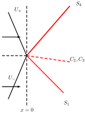
Figure 1. An unperturbed four-wave configuration, consisting of two shocks $S_{1}$ and $S_{4}$, one vortex sheet $C_{2}$, and one entropy wave $C_{3}$

The stability problem involving supersonic flows with a single shock past a Lipschitz wedge has been solved in Chen-Zhang-Zhu [11] (also see Chen-Li [9]). The stability problem involving supersonic flows with vortex sheets and entropy waves over a Lipschitz wall has been solved in Chen-Zhang-Zhu [12]. See also Chen-Kuang-Zhang [8] for the stability of two-dimensional steady supersonic exothermically reacting Euler flow past Lipschitz bending walls.

The case of an initial configuration involving two shocks is treated in [21], by using the method of front tracking, for more general equations, under the finiteness and stability conditions. We think that, with the estimates of Riemann solutions involving more than two strong waves, the estimates on the reflection coefficients of wave interactions should play a similar role so that the method of front tracking may be used.

In this paper, it is proved that steady four-wave configurations in supersonic flow are stable in structure globally, even under the BV perturbation of the incoming flow in the flow direction. In order to achieve this, we first formulate the problem as the Cauchy problem (initial value problem) in the flow direction, then develop a modified Glimm difference scheme similar to those in [11, 12] from the original Glimm scheme in [19] for one-dimensional hyperbolic conservation laws, and further identify a Glimm-type functional to obtain the required BV estimates by tracing the interactions not only between the strong shocks and weak waves, but also between the strong vortex sheet/entropy wave and weak waves carefully. The key feature of the Euler equations is that the reflection coefficient is always less than $1$, when a weak wave of different family interacts with the vortextsheets/entropy wave or the shock wave, which is crucial to guarantee that the Glimm functional is decreasing. Then these estimates are employed to establish the convergence of the approximate solutions to a global entropy solution, close to the background solution of steady four-wave configuration.

This paper is organized as follows: In §2, we first formulate the stability of multi-wave configurations as the Cauchy problem (initial value problem) in the flow direction for the Euler equations (1.1) and then state the main theorem of this paper. In §3, some fundamental properties of system (1.1) and the analysis of the Riemann solutions are presented, which are used in the subsequent sections. In §4, we make estimates on the wave interactions, especially between the strong and weak waves, and identify the key feature of the Euler equations that the reflection coefficient is always less than $1$, when a weak wave of different family interacts with the vortex sheet/entropy wave or the shock wave. In §5, we develop a modified Glimm difference scheme, based on the ones in [11, 12], to construct a family of approximate solutions, and establish necessary estimates that will be used later to obtain its convergence to an entropy solution of the Cauchy problem (1.1) and (2.1). In §6, we show the convergence of the approximate solutions to an entropy solution, close to the background solution of steady four-wave configuration.

2. Formulation of the Problem and Main Theorem

In this section, we formulate the stability problem for the steady four-wave configurations as the Cauchy problem (initial value problem) in the flow direction for the Euler equations (1.1) and then state the main theorem of this paper.

2.1. Stability problem

We focus on the stability problem of the four-wave configurations consisting of two strong shocks, one strong vortex sheet, and one entropy wave for the supersonic Euler flows governed by system (1.1) for $U=(u,v,p,\rho)$. More precisely, we consider a background solution $\overline{U}:\mathbb{R}^{2}_{+}\rightarrow\mathbb{R}$ that consists of four constant states:

$$U_{b}=(u_{b},v_{b},p_{b},\rho_{b}),$$

$$U_{m1}=(u_{m1},0,p_{m1},\rho_{m1}),$$

$$U_{m2}=(u_{m2},0,p_{m2},\rho_{m2}),$$

$$U_{a}=(u_{a},v_{a},p_{a},\rho_{a}),$$

where $u_{j}>c_{j}$ for all $j\in\{a,m_{1},m_{2},b\}$ with the sonic speed of state $U_{j}$:

$$c_{j}=\sqrt{\frac{\gamma p_{j}}{\rho_{j}}},$$

and state $U_{m1}$ connects to $U_{b}$ by a strong $1$–shock of speed $\sigma_{10}$, $U_{m1}$ connects to $U_{m2}$ by a strong $2$–vortex sheet and a strong $3$–entropy wave of strengths $(\sigma_{20},\sigma_{30})$, and $U_{a}$ connects to $U_{m2}$ by a strong $4$–shock of speed $\sigma_{40}$; see Figure 2.

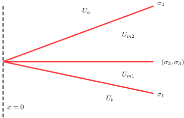
Figure 2. The background solution $\overline{U}$, consisting of four waves and four constant states

We are interested in the stability of the background solution $\overline{U}$ of steady four-wave configuration, under small $BV$ perturbations of the incoming flow as the initial data, to see whether it leads to entropy solutions containing similar strong four-wave configurations, close to the background solution $\overline{U}$. That is, the stability problem can be formulated as the following Cauchy problem (initial value problem) for the Euler equations (1.1) with the Cauchy data:

$$\left.U\right|_{x=0}=U_{0},$$ (2.1)

where $U_{0}\in\mathrm{BV}(\mathbb{R})$ is a small perturbation function close to $\overline{U}(\cdot,0)$ in $BV$.

The main theorem of this paper is the following:

Theorem 2.1 (Existence and Stability).

There exist $\epsilon>0$ and $C>0$ such that, if $U_{0}\in BV(\mathbb{R})$ satisfies

$$\mathrm{TV}\{U_{0}(\cdot)-\overline{U}(0,\cdot)\}<\epsilon,$$

then there are four functions:

$$U\in BV_{loc}(\mathbb{R}^{2}_{+})\cap L^{\infty}(\mathbb{R}^{2}_{+}),\qquad\,\chi_{i}\in\mathrm{Lip}(\mathbb{R}_{+};\mathbb{R}_{+})\quad\mbox{for $i=1,2,3,4$,}$$

such that

1. $U$ is a global entropy solution of system (1.1) in $\mathbb{R}^{2}_{+}$, satisfying the initial condition (2.1);

2. Curves $\{y=\chi_{i}(x)\}$, $i=1,2,3,4$, are a strong $1$–shock, a combined strong $2$–vortex sheet and $3$–entropy wave ($\chi_{2,3}:=\chi_{2}=\chi_{3}$), and a strong $4$–shock, respectively, all emanating from the origin, with

   $$\left\lvert U(x,y)|_{\{y<\chi_{1}(x)\}}-U_{b}\right\rvert<C\epsilon,$$

   $$\left\lvert U(x,y)|_{\{\chi_{1}(x)<y<\chi_{2,3}(x)\}}-U_{m1}\right\rvert<C\epsilon,$$

   $$\left\lvert U(x,y)|_{\{\chi_{2,3}(x)<y<\chi_{4}(x)\}}-U_{m2}\right\rvert<C\epsilon,$$

   $$\left\lvert U(x,y)|_{\{\chi_{4}(x)<y\}}-U_{a}\right\rvert<C\epsilon.$$

In §2–§6, we prove this main theorem and related properties of the global solution in $BV$.

3. Riemann Problems and Solutions

This section includes some fundamental properties of system (1.1) and some analysis of the Riemann solutions, which will be used in the subsequent sections; see also [11, 12].

3.1. Euler equations

With $U=(u,v,p,\rho)$, the Euler system can be written in the following conservation form:

$$W(U)_{x}+H(U)_{y}=0,$$ (3.1)

where

$$W(U)=(\rho u,\rho u^{2}+p,\rho uv,\rho u(h+\frac{u^{2}+v^{2}}{2})),\,\,H(U)=(\rho v,\rho uv,\rho v^{2}+p,\rho v(h+\frac{u^{2}+v^{2}}{2})),$$ (3.2)

and $h=\frac{\gamma p}{(\gamma-1)\rho}$. For a smooth solution $U(x,y)$, (3.2) is equivalent to

$$\nabla_{U}W(U)U_{x}+\nabla_{U}H(U)U_{y}=0,$$ (3.3)

so that the eigenvalues of (3.2) are the roots of the fourth order polynomial:

$$\mathrm{det}\left(\lambda\nabla_{U}W(U)-\nabla_{U}H(U)\right),$$ (3.4)

which are solutions of the equation:

$$(v-\lambda u)^{2}\left((v-\lambda u)^{2}-c^{2}(1+\lambda^{2})\right)=0,$$ (3.5)

where $c=\sqrt{\gamma p/\rho}$ is the sonic speed. If the flow is supersonic, i.e. $u^{2}+v^{2}>c^{2}$, system (1.1) is hyperbolic. In particular, when $u>c$, system (1.1) has the following four eigenvalues in the $x$–direction:

$$\lambda_{j}=\frac{uv+(-1)^{j}c\sqrt{u^{2}+v^{2}-c^{2}}}{u^{2}-c^{2}}\quad\mbox{for $j=1,4$};\,\,\qquad\lambda_{i}=\frac{v}{u}\quad\mbox{for $i=2,3$},$$ (3.6)

with four corresponding linearly independent eigenvectors:

$$\mathbf{r}_{j}=\kappa_{j}(-\lambda_{j},1,\rho(\lambda_{j}u-v),\frac{\rho(\lambda_{j}u-v)}{c^{2}})^{\top}\qquad\mbox{for $j=1,4$},$$ (3.7)

$$\mathbf{r}_{2}=(u,v,0,0)^{\top},\qquad\mathbf{r}_{3}=(0,0,0,\rho)^{\top},$$

where $\kappa_{j}$ are chosen to ensure that $\mathbf{r}_{j}\cdot\nabla\lambda_{j}=1$ for $j=1,4$, since the first and fourth characteristic fields are always genuinely nonlinear, and the second and third are linearly degenerate.

In particular, at a state $U=(u,0,p,\rho)$,

$$\lambda_{2}(U)=\lambda_{3}(U)=0,\qquad\lambda_{1}(U)=-\frac{c}{\sqrt{u^{2}-c^{2}}}=-\lambda_{4}(U)<0.$$

Definition 3.1.

$U\in BV(\mathbb{R}^{2}_{+})$ is called an entropy solution of (1.1) and (2.1) if

1. $U$ satisfies the Euler equations (1.1) in the distributional sense and (2.1) in the trace sense;

2. $U$ satisfies the following entropy inequality:

   $$(\rho uS)_{x}+(\rho vS)_{y}\leq 0$$ (3.8)

   in the distributional sense in $\mathbb{R}^{2}_{+}$, including the boundary.

3.2. Wave curves in the phase space

In this subsection, based on [11, pp. 297–298] and [12, pp. 1666–1667], we look at the basic properties of nonlinear waves.

We focus on the region, $\{u>c\}$, in the state space, especially in the neighborhoods of $U_{j}$ in the background solution.

We first consider self-similar solutions of (1.1):

$$(u,v,p,\rho)(x,y)=(u,v,p,\rho)(\xi),\qquad\xi=\frac{y}{x},$$

which connect to a state $U_{0}=(u_{0},v_{0},p_{0},v_{0})$. We find that

$$\mathrm{det}\big{(}\xi\nabla_{U}W(U)-\nabla_{U}H(U)\big{)}=0,$$ (3.9)

which implies

$$\xi=\lambda_{i}=\frac{v}{u}\quad\mbox{for $i=2,3$},\quad\text{or}\quad\xi=\lambda_{j}=\frac{uv+(-1)^{j}c\sqrt{u^{2}+v^{2}-c^{2}}}{u^{2}-c^{2}}\quad\mbox{for $j=1,4.$}$$

First, for the cases $i=2,3$, we obtain

$$dp=0,\quad vdu-udv=0.$$ (3.10)

This yields the following curves $C_{i}(U_{0})$ in the phase space through $U_{0}$:

$$C_{i}(U_{0}):\quad p=p_{0},\quad w=\frac{v}{u}=\frac{v_{0}}{u_{0}}\,\,\qquad\mbox{for $i=2,3$},$$ (3.11)

which describe compressible vortex sheets $(i=2)$ and entropy waves $(i=3)$. More precisely, we have a vortex sheet governed by

$$C_{2}(U_{0}):\,U=(u_{0}e^{\sigma_{2}},v_{0}e^{\sigma_{2}},p_{0},\rho_{0})^{\top}$$ (3.12)

with strength $\sigma_{2}$ and slope $\frac{v_{0}}{u_{0}}$, which is determined by

$$\frac{dU}{d\sigma_{2}}=\mathbf{r_{2}}(U),\qquad U|_{\sigma_{2}=0}=U_{0};$$

and an entropy wave governed by

$$C_{3}(U_{0}):\,U=(u_{0},v_{0},p_{0},\rho_{0}e^{\sigma_{3}})^{\top}$$ (3.13)

with strength $\sigma_{3}$ and slope $\frac{v_{0}}{u_{0}}$, which is determined by

$$\frac{dU}{d\sigma_{3}}=\mathbf{r_{3}}(U),\qquad U|_{\sigma_{3}=0}=U_{0}.$$

For $j=1,4$, we obtain the $j$th rarefaction wave curve $R_{j}(U_{0})$, $j=1,4$, in the phase space through $U_{0}$:

$$R_{j}(U_{0}):\,dp=c^{2}d\rho,\,du=-\lambda_{j}dv,\,\rho(\lambda_{j}u-v)dv=dp\,\qquad\text{for }\rho<\rho_{0},u>c,\,j=1,4.$$ (3.14)

For shock wave solutions, the Rankine-Hugoniot conditions for (1.1) are

$$s\left[\rho u\right]=\left[\rho v\right],$$ (3.15)

$$s\left[\rho u^{2}+p\right]=\left[\rho uv\right],$$ (3.16)

$$s\left[\rho uv\right]=\left[\rho v^{2}+p\right],$$ (3.17)

$$s\big{[}\rho u\big{(}h+\frac{u^{2}+v^{2}}{2}\big{)}\big{]}=\big{[}\rho v\big{(}h+\frac{u^{2}+v^{2}}{2}\big{)}\big{]},$$ (3.18)

where the jump symbol $\left[\,\cdot\,\right]$ stands for the value of the front state minus that of the back state. We find that

$$(v_{0}-su_{0})^{2}\big{(}(v_{0}-su_{0})^{2}-\overline{c}^{2}(1+s^{2})\big{)}=0,$$

where $\overline{c}^{2}=\frac{c_{0}^{2}}{b}$ and $b=\frac{\gamma+1}{2}-\frac{\gamma-1}{2}\frac{\rho}{\rho_{0}}$. This implies

$$s=s_{i}=\frac{v_{0}}{u_{0}}\qquad\mbox{for $i=2,3$},$$ (3.19)

or

$$s=s_{j}=\frac{u_{0}v_{0}+(-1)^{j}\overline{c}\sqrt{u_{0}^{2}+v_{0}^{2}-\overline{c}^{2}}}{u_{0}^{2}-\overline{c}^{2}}\qquad\mbox{for $j=1,4$},$$ (3.20)

where $u_{0}>\overline{c}$ for small shocks.

For $s_{i}$, $i=2,3$, in (3.15)–(3.18), we obtain the same $C_{i}(U_{0})$, $i=2,3$, defined in (3.12)–(3.13), since the corresponding fields are linearly degenerate.

On the other hand, for $s_{j},j=1,4$, in (3.15)–(3.18), we obtain the $j$th shock wave curve $S_{j}(U_{0})$, $j=1,4$, through $U_{0}$:

$$S_{j}(U_{0}):\,\left[p\right]=\frac{c_{0}^{2}}{b}\left[\rho\right],\,\left[u\right]=-s_{j}\left[v\right],\,\rho_{0}(s_{j}u_{0}-v_{0})\left[v\right]=\left[p\right]\qquad\,\text{for $\rho>\rho_{0},u>c,\,\,j=1,4$},$$ (3.21)

where $\rho_{0}<\rho$ is equivalent to the entropy condition (3.8) on the shock wave. We also know that $S_{j}(U_{0})$ agrees with $R_{j}(U_{0})$ up to second order and that

$$\left.\frac{d\sigma_{1}}{d\rho}\right|_{S_{1}(U_{0})}<0,\qquad\left.\frac{d\sigma_{4}}{d\rho}\right|_{S_{4}(U_{0})}>0.$$ (3.22)

The entropy inequality (3.8) is equivalent to the following:

$$\lambda_{j}(\text{above})<\,\sigma_{j}<\lambda_{j}(\text{below})\qquad\mbox{for $j=1,4$},$$ (3.23)

$$\sigma_{1}<\lambda_{2,3}(\text{below}),$$

$$\lambda_{2,3}(\text{above})<\,\sigma_{4};$$

see [11, pp. 269–270, pp. 297–298] for the details.

3.3. Riemann problems

We consider the Riemann problem for (1.1):

$$\left.U\right|_{x=x_{0}}=\begin{cases}U_{a},&\,\,\,y>y_{0},\\ U_{b},&\,\,\,y<y_{0},\end{cases}$$ (3.24)

where $U_{a}$ and $U_{b}$ are constant states, regarded as the above and below state with respect to line $y=y_{0}$.

3.3.1. Riemann problem only involving weak waves

Following Lax [20], we can parameterize any physically admissible wave curve in a neighborhood of a constant state $U_{0}$.

Lemma 3.1.

Given $U_{0}\in\mathbb{R}^{4}$, there exists a neighborhood $O_{\epsilon}(U_{0})$ such that, for all $U_{1},U_{2}\in O_{\epsilon}(U_{0})$, the Riemann problem (3.24) admits a unique admissible solution consisting of four elementary waves. In addition, state $U_{2}$ can be represented by

$$U_{2}=\Phi(\alpha_{4},\alpha_{3},\alpha_{2},\alpha_{1};U_{1})$$ (3.25)

with

$$\Phi(0,0,0,0;U_{1})=U_{1},$$

$$\partial_{\alpha_{i}}\Phi(0,0,0,0;U_{1})=\mathbf{r}_{i}(U_{1})\qquad\mbox{for $i=1,2,3,4$}.$$

From now on, we denote $\{U_{1},U_{2}\}=(\alpha_{1},\alpha_{2},\alpha_{3},\alpha_{4})$ as a compact way to write the representation of (3.25).

We also note that the renormalization factors $\kappa_{j}$ in (3.7) have been used to ensure that $\mathbf{r}_{j}\cdot\nabla\lambda_{j}=1$ in a neighborhood of any unperturbed state $U_{0}=(u_{0},0,p_{0},\rho_{0})$ with $u_{0}>0$, such as $U_{m1}$ or $U_{m2}$:

Lemma 3.2.

At any state $U_{0}=(u_{0},0,p_{0},\rho_{0})$ with $u_{0}>0$,

$$\kappa_{1}(U_{0})=\kappa_{4}(U_{0})>0,$$

which also holds in a neighborhood of $U_{0}$.

Also, since $\nabla_{U}\Phi(0,0,0,0;U_{1})$ is equal to the identity, by the implicit function theorem, we can find $\tilde{\Phi}$ (after possibly shrinking $O_{\epsilon}(U_{0})$) such that, in the above situation, we can represent

$$U_{1}=\tilde{\Phi}(\alpha_{4},\alpha_{3},\alpha_{2},\alpha_{1};U_{2}).$$

Differentiating the relation:

$$\tilde{\Phi}(\alpha_{4},\alpha_{3},\alpha_{2},\alpha_{1};\Phi(\alpha_{4},\alpha_{3},\alpha_{2},\alpha_{1};U_{1}))=U_{1}$$

and using that

$$\tilde{\Phi}(0,0,0,0;U_{2})=U_{2},$$

we deduce

$$\partial_{\alpha_{i}}\tilde{\Phi}(0,0,0,0;U_{2})=-\mathbf{r}_{i}(U_{2})\qquad\mbox{for $i=1,2,3,4$}.$$

This will be used later in §4. We exploit the symmetries between the shock polar and the reverse shock polar, and the symmetry between the $1$-shock polar and the reverse $4$-shock polar to allow for more concise arguments.

3.3.2. Riemann problem involving a strong $1$–shock

The results here are based on those in §6.1.4 of [11], with small changes for our requirements.

For a fixed $U_{1}$, when $U_{2}\in S_{1}(U_{1})$, we use $\{U_{1},U_{2}\}=(\sigma_{1},0,0,0)$ to denote the $1$–shock that connects $U_{1}$ to $U_{2}$ with speed $\sigma_{1}$.

Lemma 3.3.

For all $U_{1}\in O_{\epsilon}(U_{b}),U_{2}\in S_{1}(U_{1})\cap O_{\epsilon}(U_{m1})$, and $\sigma_{1}\in O_{\hat{\epsilon}}(\sigma_{10})$ with $\{U_{1},U_{2}\}=(\sigma_{1},0,0,0)$,

$$\sigma_{1}<0,\qquad u_{1}<u_{2}<\big{(}1+\frac{1}{\gamma}\big{)}u_{1}.$$

Proof.

We follow the same steps as [11, pp. 273]. First, by (3.20),

$$\sigma_{10}=-\frac{\overline{c}}{\sqrt{u_{m1}^{2}-\overline{c}^{2}}}<0.$$

Now, from the Rankine-Hugoniot conditions (3.15)–(3.18),

$$\sigma_{10}(\rho_{b}u_{b}-\rho_{m1}u_{m1})=\rho_{b}v_{b},$$ (3.26)

$$\sigma_{10}\big{(}\rho_{b}u_{b}^{2}-\rho_{m1}u^{2}_{m1}+p_{b}-p_{m1}\big{)}=\rho_{b}v_{b}u_{b}.$$ (3.27)

Thus, using (3.26)–(3.27),

$$p_{m1}-p_{b}=\rho_{m1}u_{m1}(u_{b}-u_{m1}),$$

so that $u_{b}>u_{m1}$ as $p_{m1}>p_{b}$. Also, since $p_{b}>0$, we have

$$\frac{1}{\gamma}\rho_{m1}c_{m1}^{2}=p_{m1}>\rho_{m1}u_{m1}(u_{b}-u_{m1}),$$

so that, as $u_{m1}>c_{m1}$,

$$u_{b}<\big{(}1+\frac{1}{\gamma}\big{)}u_{m1}.$$

The result now follows by continuity. ∎

Lemma 3.4.

Let

$$A:=\nabla_{U}H(U_{m1})-\sigma_{10}\nabla_{U}W(U_{m1}),$$

and

$$P:=u_{m1}\Big{(}h_{b}+\frac{u_{b}^{2}+v_{b}^{2}}{2}-\frac{u_{m1}^{2}}{2}\Big{)}+\Big{(}\frac{c_{m1}^{2}}{\gamma-1}+u_{m1}^{2}\Big{)}(u_{m1}-u_{b}).$$

Then

$$\mathrm{det}A>0,\quad\mathrm{det}(A\mathbf{r_{4}},A\mathbf{r_{3}},A\mathbf{r_{2}},A\mathbf{r_{1}})|_{U=U_{m1}}>0,$$

$$\mathrm{det}(A\mathbf{r_{4}},A\mathbf{r_{3}},A\mathbf{r_{2}},A\partial_{\sigma_{1}}G_{1}(\sigma_{10},U))|_{U=U_{m1}}>0.$$

Proof.

We omit the full calculations, which can be found at [11, pp. 299–300]. We use Lemma 3.3, along with the first and fourth Rankine-Hugoniot conditions (3.15) and (3.18), to deduce that $P>0$. We then use Lemma 3.3 and the entropy condition (3.23) to deduce

$$\mathrm{det}A=\frac{\sigma_{10}^{2}\rho_{m1}^{3}u_{m1}^{3}}{\gamma-1}\left(\lambda_{1}^{2}(U_{m1})-\sigma_{10}^{2}\right)\left(u^{2}_{m1}-c_{m1}^{2}\right)>0,$$

$$\mathrm{det}(A\mathbf{r_{4}},A\mathbf{r_{3}},A\mathbf{r_{2}},A\partial_{\sigma_{1}}G_{1}(\sigma_{10},U))|_{U=U_{m1}}$$

$$\quad=\frac{\kappa_{4}(U_{m1})^{2}\sigma_{10}\rho_{b}v_{b}\rho_{m1}^{3}u_{m1}^{2}}{\lambda_{4}(U_{m1})}\big{(}\sigma_{10}-\lambda_{4}(U_{m1})\big{)}\big{(}u_{m1}\lambda_{4}(U_{m1})P+\sigma_{10}u_{m1}Q\big{)}>0,$$

where $Q=-\frac{c_{+}^{2}}{\gamma-1}<0$. ∎

Lemma 3.5.

There exists a neighborhood $O_{\epsilon}(U_{b})\times O_{\hat{\epsilon}}(\sigma_{10})$ such that, for each $U_{0}\in O_{\epsilon}(U_{b})$, the shock polar $S_{1}(U_{b})$ can be parameterized locally for the state which connects to $U_{0}$ by a shock of speed $\sigma_{10}$ from above as

$$\sigma_{1}\mapsto G_{1}(\sigma_{1},U_{0})\,\,\qquad\text{for }\,\,|\sigma_{1}-\sigma_{10}|<\hat{\epsilon}.$$

Proof.

It suffices to solve

$$\sigma_{1}\big{(}W(U)-W(U_{0})\big{)}-\big{(}H(U)-H(U_{0})\big{)}=0$$

for $U$ in terms of $\sigma_{1}$ and $U_{0}$, with the knowledge that $(U_{0},\sigma_{1},U)=(U_{b},\sigma_{10},U_{m_{1}})$ is a solution. We see that

$$\mathrm{det}\big{(}\nabla_{U}(\sigma(W(U)-W(U_{0}))-(H(U)-H(U_{0})))\big{)}\bigg{|}_{U_{0}=U_{b},\sigma_{1}=\sigma_{10},U=U_{m1}}=\mathrm{det}A>0.$$

Then the result follows by the implicit function theorem. ∎

3.3.3. Riemann problem involving a strong $4$–shock

We now extend our results about $1$–shocks to $4$–shocks by symmetry. For a fixed $U_{1}$, when $U_{2}\in S_{4}(U_{1})$, we use $\{U_{1},U_{2}\}=(0,0,0,\sigma_{4})$ to denote the $4$–shock that connects $U_{1}$ to $U_{2}$ with speed $\sigma_{4}$. The only difference is the formula for $\sigma_{4}$.

Lemma 3.6.

For all $U_{1}\in O_{\epsilon}(U_{m2}),U_{2}\in O_{\epsilon}(U_{a})\cap S_{1}(U_{1})$, and $\sigma_{3}\in O_{\hat{\epsilon}}(\sigma_{40})$ with $\{U_{1},U_{2}\}=(0,0,0,\sigma_{4})$,

$$\sigma_{4}>0,\qquad u_{1}<u_{2}<\big{(}1+\frac{1}{\gamma}\big{)}u_{1}.$$

Proof.

Note that, by (3.23),

$$\sigma_{4}=\frac{u_{a}v_{a}+\overline{c}\sqrt{u_{a}^{2}+v_{a}^{2}-\overline{c}^{2}}}{u_{a}^{2}-\overline{c}^{2}}>0.$$

Since we have the same Rankine-Hugoniot conditions as in Lemma 3.3, with $u_{m2}$ and $u_{a}$ taking the roles of $u_{m1}$ and $u_{b}$, respectively, the proof follows identically. ∎

Lemma 3.7.

There exists a neighborhood $O_{\epsilon}(U_{a})\times O_{\hat{\epsilon}}(\sigma_{40})$ such that, for each $U_{0}\in O_{\epsilon}(U_{a})$, the reverse shock polar $\tilde{S}_{2}(U_{0})$ – the set of states that connect to $U_{0}$ by a strong $4$–shock from below – can be parameterized locally for the state which connects to $U_{0}$ by a shock of speed $\sigma_{40}$ as

$$\sigma_{4}\mapsto G_{4}(\sigma_{4},U_{0}),$$

with $G_{4}\in C^{2}$ near $(\sigma_{40},U_{m2})$.

3.3.4. Riemann problem involving strong vortex sheets and entropy waves

We now look at the interaction between weak waves and the strong vortex sheet/entropy wave, based on those in §2.5 of [12]. For any $U_{1}\in O_{\epsilon}(U_{m1})$ and $U_{2}\in O_{\epsilon}(U_{m2})$, we use $\{U_{1},U_{2}\}=(0,\sigma_{2},\sigma_{3},0)$ to denote the strong vortex sheet and entropy wave that connect $U_{1}$ to $U_{2}$ with strength $(\sigma_{2},\sigma_{3})$. That is,

$$U_{\rm mid}=\Phi_{2}(\sigma_{2},U_{1})=(u_{1}e^{\sigma_{2}},v_{1}e^{\sigma_{2}},p_{1},\rho_{1}),\,\,U_{2}=\Phi(\sigma_{3},U_{\rm mid})=(u_{\rm mid},v_{\rm mid},p_{\rm mid},\rho_{\rm mid}e^{\sigma_{3}}).$$

In particular, we have

$$U_{2}=(u_{1}e^{\sigma_{2}},v_{1}e^{\sigma_{2}},p_{1},\rho_{1}e^{\sigma_{3}}).$$

By a straightforward calculation, we have

Lemma 3.8.

For

$$G_{2,3}(\sigma_{3},\sigma_{2},U):=\Phi_{3}(\sigma_{3};\Phi_{2}(\sigma_{2};U))=(e^{\sigma_{20}}u,e^{\sigma_{20}}v,p,e^{\sigma_{30}}\rho)\qquad\mbox{for any $U\in O_{\epsilon}(U_{m1})$},$$

then

$$\partial_{\sigma 2}G_{2,3}(\sigma_{3},\sigma_{2};U) =(ue^{\sigma_{2}},ve^{\sigma_{2}},0,0)^{\top},$$

$$\partial_{\sigma 3}G_{2,3}(\sigma_{3},\sigma_{2};U) =(0,0,0,\rho e^{\sigma_{3}})^{\top},$$

$$\nabla_{U}G_{2,3}(\sigma_{3},\sigma_{2},U) =\mathrm{diag}(e^{\sigma_{2}},e^{\sigma_{2}},1,e^{\sigma_{3}}).$$

The next property allows us to estimate the strength of reflected weak waves in the interactions between the strong vortex sheet/entropy wave and weak waves:

Lemma 3.9.

The following holds:

$$\mathrm{det}\left(\mathbf{r}_{4}(U_{m2}),\partial_{\sigma_{3}}G_{2,3}(\sigma_{30},\sigma_{20};U_{m1}),\partial_{\sigma_{2}}G_{2,3}(\sigma_{30},\sigma_{20};U_{m1}),\nabla_{U}G(\sigma_{30},\sigma_{20},U_{m1})\cdot\mathbf{r}_{1}(U_{1})\right)>0.$$

Proof.

By a direct calculation,

$$\mathrm{det}\left(\mathbf{r}_{4}(U_{m2}),\partial_{\sigma_{3}}G_{2,3}(\sigma_{30},\sigma_{20};U_{m1}),\partial_{\sigma_{2}}G_{2,3}(\sigma_{30},\sigma_{20};U_{m1}),\nabla_{U}G(\sigma_{30},\sigma_{20},U_{m1})\cdot\mathbf{r}_{1}(U_{1})\right)$$

$$=\kappa_{1}(U_{m1})\kappa_{4}(U_{m2})\left|\begin{array}[]{cccc}\lambda_{4}(U_{m2})&0&u_{m1}e^{\sigma_{20}}&-e^{\sigma_{20}}\lambda_{1}(U_{m1})\\[5.69054pt] 1&0&0&e^{\sigma{20}}\\[5.69054pt] \rho_{m2}u_{m2}\lambda_{4}(U_{m2})&0&0&\rho_{m1}u_{m1}\lambda_{1}(U_{m1})\\[5.69054pt] \frac{\rho_{m2}u_{m2}\lambda_{4}(U_{m2})}{c_{m2}^{2}}&\rho_{m1}e^{\sigma_{30}}&0&e^{\sigma_{30}}\frac{\rho_{m1}u_{m1}\lambda_{1}(U_{m1})}{c_{m1}^{2}}\end{array}\right|$$

$$=\kappa_{1}(U_{m1})\kappa_{4}(U_{m2})\rho_{m1}^{2}u_{m1}^{2}e^{\sigma_{20}+\sigma_{30}}\left(\lambda_{4}(U_{m2})e^{2\sigma_{20}+\sigma_{30}}+\lambda_{4}(U_{m1})\right)>0.$$

∎

4. Estimates on the Wave Interactions

In this section, we make estimates on the wave interactions, especially between the strong and weak waves. This is based on those in §3 of [11, 12], with new estimates for the strong $4$–shock.

Below, $M>0$ is a universal constant which is understood to be large, and $O_{\epsilon}(U_{i})$ for $i\in\{a,m1,m2,b\}$ is a universal small neighborhood of $U_{i}$ which is understood to be small. Each of them depends only on the system, which may be different at each occurrence.

Figure 3. Interaction estimates

4.1. Preliminary identities

To make later arguments more concise, we now state some elementary identities here to be used later; these are simple consequences of the fundamental theorem of calculus.

Lemma 4.1.

The following identities hold:

• If $f\in C^{1}([a,b])$ with $a<0<b$, then, for any $x\in[a,b]$,

  $$f(x)-f(0)=x\int_{0}^{1}f_{x}(rx)\,dr;$$

• If $g\in C^{2}([a,b]^{2})$ with $a<0<b$, then, for any $(x,y)\in[a,b]^{2}$,

  $$f(x,y)-f(x,0)-f(0,y)+f(0,0)=xy\int_{0}^{1}\int_{0}^{1}f_{xy}(rx,sy)\,dr\,ds;$$

• If $f\in C^{1}([a,b])$, then

  $$f(x)=f(0)+O(1)|x|;$$

• If $f\in C^{2}([a,b]^{3})$, then

  $$f(x,y,z)=f(x,0,0)+f(0,y,z)-f(0,0,0)+O(1)|x|(|y|+|z|);$$

• If $g\in C^{2}([a,b]^{4})$, then

  $$g(x,y,z,w)=g(x,0,0,0)+g(0,y,z,w)-g(0,0,0,0)+O(1)|x|(|y|+|z|+|w|).$$

4.2. Estimates on weak wave interactions

We have the following standard proposition; see, for example, [23, Chapter 19] for the proof. Note that, in our analysis of the Glimm functional, we only require the estimates for the cases where the waves are approaching.

Proposition 4.1.

Suppose that $U_{1},U_{2}$, and $U_{3}$ are three states in a small neighborhood of a given state $U_{0}$ with

$$\{U_{1},U_{2}\} =(\alpha_{1},\alpha_{2},\alpha_{3},\alpha_{4}),$$

$$\{U_{2},U_{3}\} =(\beta_{1},\beta_{2},\beta_{3},\beta_{4}),$$

$$\{U_{1},U_{3}\} =(\gamma_{1},\gamma_{2},\gamma_{3},\gamma_{4}).$$

Then

$$\gamma_{i}=\alpha_{i}+\beta_{i}+O(1)\Delta(\alpha,\beta)$$ (4.1)

with

$$\Delta(\alpha,\beta)=|\alpha_{4}||\beta_{1}|+|\alpha_{3}||\beta_{1}|+|\alpha_{2}||\beta_{1}|+|\alpha_{4}||\beta_{2}|+|\alpha_{4}||\beta_{3}|+\sum_{j=1,4}\Delta_{j}(\alpha,\beta),$$

where

$$\Delta_{j}(\alpha,\beta)=\begin{cases}0,&\,\,\alpha_{j}\geq 0,\beta_{j}\geq 0,\\ |\alpha_{j}||\beta_{j}|,&\,\,\text{otherwise}.\end{cases}$$

4.3. Estimates on the interaction between the strong vortex sheet/entropy wave and weak waves

We now derive an interaction estimate between the strong vortex sheet/entropy wave and weak waves. The properties that $|K_{vb1}|<1$ in (4.2) and $|K_{va4}|<1$ in (4.5) will be critical in the proof that the Glimm functional is decreasing.

Proposition 4.2.

Let $U_{1},U_{2}\in O_{\epsilon}(U_{m1})$ and $U_{3}\in O_{\epsilon}(U_{m2})$ with

$$\{U_{1},U_{2}\}=(0,\alpha_{2},\alpha_{3},\alpha_{4})\qquad\text{and}\qquad\{U_{2},U_{3}\}=(\beta_{1},\sigma_{2},\sigma_{3},0),$$

there is a unique $(\delta_{1},\sigma^{\prime}_{2},\sigma^{\prime}_{3},\delta_{4})$ such that

$$\{U_{1},U_{3}\}=(\delta_{1},\sigma^{\prime}_{2},\sigma^{\prime}_{3},\delta_{4}),$$

and

$$\delta_{1} =\beta_{1}+K_{vb1}\alpha_{4}+O(1)\Delta^{\prime},$$

$$\sigma^{\prime}_{2} =\sigma_{2}+\alpha_{2}+K_{vb2}\alpha_{4}+O(1)\Delta^{\prime},$$

$$\sigma^{\prime}_{3} =\sigma_{3}+\alpha_{3}+K_{vb3}\alpha_{4}+O(1)\Delta^{\prime},$$

$$\delta_{4} =K_{vb4}\alpha_{4}+O(1)\Delta^{\prime},$$

with

$$\Delta^{\prime}=|\beta_{1}|(|\alpha_{2}|+|\alpha_{3}|),\qquad|K_{vb1}|<1,\qquad\sum_{j=2}^{4}|K_{vbj}|\leq M.$$ (4.2)

Proof.

This proof is the same as [12, pp. 1673], with additional terms. We need to solve for $(\delta_{1},\sigma_{2}^{\prime},\sigma_{3}^{\prime},\delta_{4})$ as a function of $(\alpha_{1},\alpha_{2},\alpha_{3},\alpha_{4},\beta_{1},\sigma_{2},\sigma_{3},\beta_{4},U_{1})$ in the following equation:

$$\Phi_{4}(\delta_{4};G_{2,3}(\sigma_{2}^{\prime},\sigma_{3}^{\prime};\Phi_{1}(\delta_{1};U_{1})))=\Phi_{4}(\beta_{4};G(\sigma_{3},\sigma_{2};\Phi_{1}(\beta_{1};\Phi(\alpha_{4},\alpha_{3},\alpha_{2},\alpha_{1};U_{1})))).$$ (4.3)

Lemma 3.9 implies

$$\left.\mathrm{det}\left(\frac{\partial\Phi_{4}(\delta_{4};G_{2,3}(\sigma_{2}^{\prime},\sigma_{3}^{\prime};\Phi_{1}(\delta_{1};U_{1})))}{\partial(\delta_{4},\sigma_{3}^{\prime},\sigma_{2}^{\prime},\delta_{1})}\right)\right|_{\delta_{4}=\delta_{1}=0,\sigma_{2}^{\prime}=\sigma_{20},\sigma_{3}^{\prime}=\sigma_{30},U_{1}=U_{m1}}\hfill$$

$$=\mathrm{det}\left(\mathbf{r}_{4}(U_{m2}),\partial_{\sigma_{3}}G_{2,3}(\sigma_{30},\sigma_{20};U_{m1}),\partial_{\sigma_{2}}G_{2,3}(\sigma_{30},\sigma_{20};U_{m1}),\nabla_{U}G(\sigma_{30},\sigma_{20},U_{m1})\cdot\mathbf{r}_{1}(U_{1})\right)$$

$$>0.\hfill$$

Note that, when $\alpha_{4}=0$, the unique solution is

$$\delta_{1}=\beta_{1},\quad\sigma^{\prime}_{2}=\sigma_{2}+\alpha_{2},\quad\sigma^{\prime}_{3}=\sigma_{3}+\alpha_{3},\quad\delta_{4}=\beta_{4},$$

so that

$$\delta_{1} =\beta_{1}+K_{vb1}\alpha_{4}+\alpha_{1}+O(1)\Delta^{\prime},$$ (4.4)

$$\delta_{4} =K_{vb4}\alpha_{4}+\beta_{4}+O(1)\Delta^{\prime},$$

$$\sigma^{\prime}_{i} =\sigma_{i}+\alpha_{i}+K_{vbi}\alpha_{4}+O(1)\Delta^{\prime}\qquad\mbox{for $i=2,3$},$$

where

$$K_{vbi}=\int_{0}^{1}\partial_{\alpha_{4}}\sigma^{\prime}_{i}(\alpha_{2},\alpha_{3},\theta\alpha_{4},\beta_{1},\sigma_{2},\sigma_{3})\,d\theta\qquad\mbox{for $i=2,3$},$$

$$K_{vbj}=\int_{0}^{1}\partial_{\alpha_{4}}\delta_{j}(\alpha_{2},\alpha_{3},\theta\alpha_{4},\beta_{1},\sigma_{2},\sigma_{3})\,d\theta\qquad\mbox{for $j=1,4$}.$$

We see that $K_{vbi}$ and $K_{bvj}$ are bounded from the formulae above. To deduce that $|K_{vb1}|<1$, we differentiate (4.3) with respect to $\alpha_{4}$ to obtain

$$\nabla_{U}G_{2,3}(\sigma_{30},\sigma_{20};U_{m1})\cdot\mathbf{r}_{4}(U_{m1})$$

$$=\partial_{\alpha_{4}}\delta_{4}\,\mathbf{r}_{4}(U_{m2})+\partial_{\alpha_{4}}\sigma^{\prime}_{3}\,\partial_{\sigma_{3}}G_{2,3}(\sigma_{30},\sigma_{20};U_{m1})+\partial_{\alpha_{4}}\sigma^{\prime}_{2}\,\partial_{\sigma 2}G_{2,3}(\sigma_{30},\sigma_{20};U_{m1})$$

$$\quad+\partial_{\alpha_{4}}\delta_{1}\,\nabla_{U}G_{2,3}(\sigma_{30},\sigma_{20};U_{m1})\cdot\mathbf{r}_{1}(U_{m1}).$$

By Lemma 3.8 and another similar calculation, we have

$$|\partial_{\alpha_{4}}\delta_{1}|$$

$$=\left\lvert\frac{\mathrm{det}\left(\mathbf{r}_{4}(U_{m2}),\partial_{\sigma_{3}}G_{2,3}(\sigma_{30},\sigma_{20};U_{m1}),\partial_{\sigma_{2}}G_{2,3}(\sigma_{30},\sigma_{20};U_{m1}),\nabla_{U}G(\sigma_{30},\sigma_{20},U_{m1})\cdot\mathbf{r}_{4}(U_{1})\right)}{\mathrm{det}\left(\mathbf{r}_{4}(U_{m2}),\partial_{\sigma_{3}}G_{2,3}(\sigma_{30},\sigma_{20};U_{m1}),\partial_{\sigma_{2}}G_{2,3}(\sigma_{30},\sigma_{20};U_{m1}),\nabla_{U}G(\sigma_{30},\sigma_{20},U_{m1})\cdot\mathbf{r}_{1}(U_{1})\right)}\right\rvert$$

$$=\left\lvert\frac{\kappa_{1}(U_{m1})\kappa_{4}(U_{m2})\rho_{m1}^{2}u_{m1}^{2}e^{\sigma_{20}+\sigma_{30}}\left(\lambda_{4}(U_{m2})e^{2\sigma_{20}+\sigma_{30}}-\lambda_{4}(U_{m1})\right)}{\kappa_{1}(U_{m1})\kappa_{4}(U_{m2})\rho_{m1}^{2}u_{m1}^{2}e^{\sigma_{20}+\sigma_{30}}\left(\lambda_{4}(U_{m2})e^{2\sigma_{20}+\sigma_{30}}+\lambda_{4}(U_{m1})\right)}\right\rvert$$

$$=\left\lvert\frac{\lambda_{4}(U_{m2})e^{2\sigma_{20}+\sigma_{30}}-\lambda_{4}(U_{m1})}{\lambda_{4}(U_{m2})e^{2\sigma_{20}+\sigma_{30}}+\lambda_{4}(U_{m1})}\right\rvert$$

$$<1.$$

∎

We can then deduce the following result by symmetry:

Proposition 4.3.

If $U_{1}\in O_{\epsilon}(U_{m2})$ and $U_{2},U_{3}\in O_{\epsilon}(U_{m1})$ with

$$\{U_{1},U_{2}\}=(0,\sigma_{2},\sigma_{3},\alpha_{4}),\qquad\{U_{2},U_{3}\}=(\beta_{1},\beta_{2},\beta_{3},0),$$

then

$$\{U_{1},U_{3}\}=(\delta_{1},\sigma^{\prime}_{2},\sigma^{\prime}_{3},\delta_{4})$$

with

$$\delta_{1} =K_{va1}\beta_{1}+O(1)\Delta^{\prime\prime},$$

$$\sigma^{\prime}_{2} =\sigma_{2}+\beta_{2}+K_{va2}\beta_{1}+O(1)\Delta^{\prime\prime},$$

$$\sigma^{\prime}_{3} =\sigma_{3}+\beta_{3}+K_{va3}\beta_{1}+O(1)\Delta^{\prime\prime},$$

$$\delta_{4} =\alpha_{4}+K_{va4}\beta_{1}+O(1)\Delta^{\prime\prime},$$

and

$$\Delta^{\prime\prime}=|\alpha_{4}|(|\beta_{2}|+|\beta_{3}|),\qquad\sum_{j=1}^{3}|K_{vaj}|\leq M,\qquad|K_{va4}|<1.$$ (4.5)

4.4. Estimates on the interaction between the strong shocks and weak waves

We now derive an interaction estimate between the strong shocks and weak waves. The properties that $|K_{1sa4}|<1$ in (4.6) and $|K_{4sb1}|<1$ in (4.14) will be critical in the proof that the Glimm functional is decreasing.

4.4.1. Interaction between the strong $1$–shock and weak waves

Proposition 4.4.

If $U_{1}\in O_{\epsilon}(U_{b})$ and $U_{2},U_{3}\in O_{\epsilon}(U_{m2})$ with

$$\{U_{1},U_{2}\}=(\sigma_{1},\alpha_{2},\alpha_{3},\alpha_{4}),\qquad\{U_{2},U_{3}\}=(\beta_{1},\beta_{2},\beta_{3},0),$$

then there exists a unique $(\sigma^{\prime}_{1},\delta_{2},\delta_{3},\delta_{4})$ such that

$$\{U_{1},U_{3}\}=(\sigma^{\prime}_{1},\delta_{2},\delta_{3},\delta_{4}).$$

Moreover,

$$\sigma^{\prime}_{1}=\sigma_{1}+K_{1sa1}\beta_{1}+O(1)\Delta^{\prime\prime},\qquad\qquad\,\delta_{2}=\alpha_{2}+\beta_{2}+K_{1sa2}\beta_{1}+O(1)\Delta^{\prime\prime},$$

$$\delta_{3}=\alpha_{3}+\beta_{3}+K_{1sa3}\beta_{1}+O(1)\Delta^{\prime\prime},\qquad\delta_{4}=\alpha_{4}+\beta_{4}+K_{1sa4}\beta_{1}+O(1)\Delta^{\prime\prime},$$

with

$$\Delta^{\prime\prime}=|\alpha_{4}|(|\beta_{1}|+|\beta_{2}|+|\beta_{3}|),\qquad|K_{1sa4}|<1,\qquad\sum_{j=1}^{3}|K_{1saj}|\leq M.$$ (4.6)

Proof.

This is similar to [11, pp. 303], with extra terms. We need to show that there exists a solution $(\sigma_{1}^{\prime},\delta_{2},\delta_{3},\delta_{4})$ to

$$\Phi(0,\beta_{3},\beta_{2},\beta_{1};\Phi(\alpha_{4},\alpha_{3},\alpha_{2},0;G_{1}(\sigma_{1};U_{1})))=\Phi(\delta_{4},\delta_{3},\delta_{2},0;G_{1}(\sigma^{\prime}_{1},U_{1})).$$ (4.7)

By Proposition 4.1, there exists $(\gamma_{4},\gamma_{3},\gamma_{2},\gamma_{1})$ as a function of $(\alpha_{2},\alpha_{3},\alpha_{4},\beta_{1},\beta_{2},\beta_{3},\beta_{4})$ such that

$$\Phi(0,\beta_{3},\beta_{2},\beta_{1};\Phi(\alpha_{4},\alpha_{3},\alpha_{2},0;G_{1}(\sigma_{1};U_{1})))=\Phi(\gamma_{4},\gamma_{3},\gamma_{2},\gamma_{1};G_{1}(\sigma_{1};U_{1}))$$ (4.8)

with

$$\gamma_{1}=\beta_{1}+O(1)\tilde{\Delta},\qquad\qquad\,\,\gamma_{2}=\alpha_{2}+\beta_{2}+O(1)\tilde{\Delta},$$ (4.9)

$$\gamma_{3}=\alpha_{3}+\beta_{3}+O(1)\tilde{\Delta},\qquad\gamma_{4}=\alpha_{4}+O(1)\tilde{\Delta},$$

where

$$\tilde{\Delta}=\Delta^{\prime\prime}+|\beta_{1}|(|\alpha_{2}|+|\alpha_{3}|+|\alpha_{4}|).$$

Thus, we may reduce (4.7) to

$$\Phi(\gamma_{4},\gamma_{3},\gamma_{2},\gamma_{1};G_{1}(\sigma_{1},U_{1}))=\Phi(\delta_{4},\delta_{3},\delta_{2},0;G_{1}(\sigma^{\prime}_{1},U_{1})).$$ (4.10)

By Lemma 3.4,

$$\mathrm{det}\left.\left(\frac{\partial\Phi(\delta_{4},\delta_{3},\delta_{2},0;G_{1}(\sigma^{\prime}_{1},U_{1}))}{\partial(\sigma_{1}^{\prime},\delta_{2},\delta_{3},\delta_{4})}\right)\right|_{\{U_{1}=U_{b},\delta_{2}=\delta_{3}=\delta_{4}=0,\sigma^{\prime}_{1}=\sigma_{10}\}}$$

$$=\frac{1}{\mathrm{det}A}\mathrm{det}(A\mathbf{r_{4}},A\mathbf{r_{3}},A\mathbf{r_{2}},A\partial_{\sigma_{1}}G_{1}(\sigma_{10};U_{b}))|_{U=U_{m1}}>0.$$

Next, observe that, when $\gamma_{1}=0$, the unique solution is $(\sigma^{\prime},\delta_{2},\delta_{3},\delta_{4})=(\sigma_{1},\gamma_{2},\gamma_{3},\gamma_{4})$. Thus, for $i=2,3,4$,

$$\sigma^{\prime}_{1}=K_{1sa1}\gamma_{1}+\sigma_{1},\qquad\delta_{i}=K_{1sai}\gamma_{1}+\gamma_{i},$$ (4.11)

where

$$K_{1sa1} =\int_{0}^{1}\partial_{\gamma_{1}}\sigma^{\prime}_{1}(t\gamma_{1},\gamma_{2},\gamma_{3},\gamma_{4},\sigma_{1},U_{1})\,dt,$$ (4.12)

$$K_{1sai} =\int_{0}^{1}\partial_{\gamma_{1}}\delta_{i}(t\gamma_{1},\gamma_{2},\gamma_{3},\gamma_{4},\sigma_{1},U_{1})\,dt\qquad\mbox{for $i=2,3,4$}.$$

To see that $|K_{1sa4}|<1$, we find that, by Lemma 3.4 and another similar computation,

$$|\partial_{\gamma_{1}}\delta_{4}| =\left\lvert\frac{\mathrm{det}(A\mathbf{r}_{1},\mathbf{A}r_{2},A\mathbf{r}_{3},A\partial_{\sigma_{1}}G_{1}(\sigma_{10},U_{b}))}{\mathrm{det}(A\mathbf{r}_{4},\mathbf{A}r_{2},A\mathbf{r}_{3},A\partial_{\sigma_{1}}G_{1}(\sigma_{10},U_{b}))}\right\rvert$$

$$=\left\lvert\frac{\sigma_{10}+\lambda_{1}(U_{m1})}{\sigma_{10}-\lambda_{1}(U_{m1})}\right\rvert\left\lvert\frac{u_{m1}\lambda_{4}(U_{m1})P+\frac{c_{m2}^{2}}{\gamma-1}\sigma_{10}u_{b}}{u_{m1}\lambda_{4}(U_{m1})P-\frac{c_{m2}^{2}}{\gamma-1}\sigma_{10}u_{b}}\right\rvert<1.$$

Now, using the expression of $\gamma$ in terms of $(\alpha,\beta)$ and absorbing the residual part of the $\tilde{\Delta}$–term into the $K_{1sai}\beta_{1}$–term, we have the desired result. ∎

We now prove a result for the case where weak waves approach the strong $1$-shock from below.

Proposition 4.5.

Suppose that $U_{1},U_{2}\in O_{\epsilon}(U_{b})$ and $U_{3}\in O_{\epsilon}(U_{m2})$ such that

$$\{U_{1},U_{2}\}=(\alpha_{1},\alpha_{2},\alpha_{3},\alpha_{4}),\qquad\{U_{2},U_{3}\}=(\sigma_{1},\beta_{2},\beta_{3},\beta_{4}).$$

Then there exists a unique $(\sigma^{\prime}_{1},\delta_{2},\delta_{3},\delta_{4})$ such that

$$\{U_{1},U_{3}\}=(\sigma^{\prime}_{1},\delta_{2},\delta_{3},\delta_{4}).$$

Moreover,

$$\sigma^{\prime}_{1}=\sigma_{1}+\sum_{j=1}^{4}K_{1sb1j}\alpha_{j},\qquad\,\,\delta_{2}=\beta_{2}+\sum_{j=1}^{4}K_{1sb2j}\alpha_{j},$$

$$\delta_{3}=\beta_{3}+\sum_{j=1}^{4}K_{1sb3j}\alpha_{j},\qquad\delta_{4}=\beta_{4}+\sum_{j=1}^{4}K_{1sb4j}\alpha_{j},$$

where

$$\sum_{i,j}|K_{1sbij}|\leq M.$$

Proof.

We need to find a solution to

$$\Phi(\delta_{4},\delta_{3},\delta_{2},0;G_{1}(\sigma^{\prime}_{1};U_{1}))=\Phi(\beta_{4},\beta_{3},\beta_{2},0;G_{1}(\sigma_{1};\Phi(\alpha_{4},\alpha_{3},\alpha_{2},\alpha_{1};U_{1}))).$$ (4.13)

By Lemma 3.4,

$$\mathrm{det}\left(\frac{\partial\Phi(\delta_{4},\delta_{3},\delta_{2},0;G_{1}(\sigma^{\prime}_{1};U_{1}))}{\partial(\sigma^{\prime}_{1},\delta_{2},\delta_{3},\delta_{4})}\right)=\mathrm{det}A>0.$$

Now the required result follows by using Lemma 4.1, and noting that $\sigma^{\prime}_{1}=\sigma_{1}$, $\alpha_{1}=\alpha_{2}=\alpha_{3}=\alpha_{4}=0$ and that $(\sigma^{\prime}_{1},\delta_{2},\delta_{3},\delta_{4})=(\sigma_{1},\beta_{2},\beta_{3},\beta_{4})$ is a solution. ∎

4.4.2. Interaction between the strong $4$–shock and weak waves

Now, by symmetry with the $1$–shock case, we deduce the following results:

Proposition 4.6.

Suppose that $U_{1}\in O_{\epsilon}(U_{m1})$ and $U_{2},U_{3}\in O_{\epsilon}(U_{m2})$ such that

$$\{U_{1},U_{2}\}=(\alpha_{1},\alpha_{2},\alpha_{3},\sigma_{4}),\qquad\{U_{2},U_{3}\}=(\beta_{1},\beta_{2},\beta_{3},\beta_{4}).$$

Then there exists a unique $(\delta_{1},\delta_{2},\delta_{3},\sigma^{\prime}_{4})$ such that

$$\{U_{1},U_{3}\}=(\delta_{1},\delta_{2},\delta_{3},\sigma^{\prime}_{4}).$$

Moreover,

$$\delta_{1}=\alpha_{1}+\sum_{j=1}^{4}K_{4sa1j}\beta_{j},\qquad\delta_{2}=\alpha_{2}+\sum_{j=1}^{4}K_{4sa2j}\beta_{j},$$

$$\delta_{3}=\alpha_{3}+\sum_{j=1}^{4}K_{4sa3j}\beta_{j},\qquad\sigma^{\prime}_{4}=\sigma_{4}+\sum_{j=1}^{4}K_{4sa4j}\beta_{j},$$

where $\sum_{i,j}|K_{4saij}|\leq M$.

Proposition 4.7.

If $U_{1},U_{2}\in O_{\epsilon}(U_{m1})$ and $U_{3}\in O_{\epsilon}(U_{a})$ with

$$\{U_{1},U_{2}\}=(0,\alpha_{2},\alpha_{3},\alpha_{4}),\qquad\{U_{2},U_{3}\}=(\beta_{1},\beta_{2},\beta_{3},\sigma_{4}),$$

then there exists a unique $(\delta_{1},\delta_{2},\delta_{3},\sigma^{\prime}_{4})$ such that

$$\{U_{1},U_{3}\}=(\delta_{1},\delta_{2},\delta_{3},\sigma^{\prime}_{4}).$$

Moreover,

$$\delta_{1}=\beta_{1}+K_{4sb1}\alpha_{4}+O(1)\Delta^{\prime\prime\prime},\qquad\qquad\,\,\delta_{2}=\beta_{2}+\alpha_{2}+K_{4sb2}\alpha_{4}+O(1)\Delta^{\prime\prime\prime},$$

$$\delta_{3}=\beta_{3}+\alpha_{3}+K_{4sb3}\alpha_{4}+O(1)\Delta^{\prime\prime\prime},\qquad\,\sigma^{\prime}_{4}=\sigma_{4}+K_{4sb4}\alpha_{4}+O(1)\Delta^{\prime\prime\prime},$$

where

$$\Delta^{\prime\prime\prime}=|\beta_{1}|(|\alpha_{2}|+|\alpha_{3}|),\qquad|K_{4sb1}|<1,\qquad\sum_{j=1}^{3}|K_{4sbj}|\leq M.$$ (4.14)

5. Approximate Solutions and BV Estimates

In this section, we develop a modified Glimm difference scheme, based on the ones in [12, 11], to construct a family of approximate solutions and establish necessary estimates that will be used later to obtain its convergence to an entropy solution to (1.1) and (2.1).

5.1. A modified Glimm scheme

For $\Delta x>0$, we define

$$\Omega_{\Delta x}=\bigcup_{k\geq 1}\Omega_{\Delta x,k},$$

where

$$\Omega_{\Delta x,k}=\{(x,y)\,:\,(k-1)\Delta x<x\leq k\Delta x\}.$$

We choose $\Delta y>0$ such that the following condition holds:

$$\frac{\Delta y}{\Delta x}>\max\Big{\{}\max_{1\leq i\leq 4}\sup_{\sigma\in O_{\hat{\epsilon}}(\sigma_{i0})}|\sigma|,\,\max_{j=1,4}\,\big{\{}\sup_{U\in O_{\epsilon}(U_{a})\cup O_{\epsilon}(U_{b})}|\lambda_{j}(U)|\big{\}},\,\sup_{U\in O_{\epsilon}(U_{m1})\cup O_{\epsilon}(U_{m2})}|\lambda_{2}(U)|\Big{\}}.$$

We also need to make sure that the strong shocks do not interact: If we take the neighborhoods small enough, there exist $a$ and $b$ with $-1<a<0<b<1$ such that

$$\sigma_{1}<\frac{\Delta y}{\Delta x}a<\lambda_{2}(U)<\frac{\Delta y}{\Delta x}b<\sigma_{4}$$

for all $U\in O_{\epsilon}(U_{m1})\cup O_{\epsilon}(U_{m2})$ and $\sigma_{i}\in O_{\hat{\epsilon}}(\sigma_{i0}),i=1,4$. Thus, a strong $1$–shock emanating from $((k-1)\Delta x,n\Delta y)$ meets $x=k\Delta x$ in the line segment $\{k\Delta x\}\times((n-1)\Delta y,(n+a)\Delta y)$, a combined strong $2$–vortex sheet/$3$–entropy wave emanating from $((k-1)\Delta x,n\Delta y)$ meets $x=k\Delta x$ in the line segment $\{k\Delta x\}\times((n+a)\Delta y,(n+b)\Delta y)$, and a strong $4$–shock emanating from $((k-1)\Delta x,n\Delta y)$ meets $x=k\Delta x$ in the line segment $\{k\Delta x\}\times((n+b)\Delta y,(n+1)\Delta y)$.

Now define

$$a_{k,n}=(n+1+\theta_{k})\Delta y,\qquad k\in\mathbb{N}_{0},\,\,n\in\mathbb{Z},\,\,n+k\equiv 1\,(\mathrm{mod}\,2),$$

where $\theta_{k}$ is randomly chosen in $(-1,1)$. We then choose

$$P_{k,n}=(k\Delta x,a_{k,n}),\qquad k\in\mathbb{N}_{0},\,\,n\in\mathbb{Z},\,\,n+k\equiv 1\,(\mathrm{mod}\,2),$$

to be the mesh points, and define the approximate solutions $U_{\Delta x,\theta}$ globally in $\Omega_{\Delta x}$ for any $\theta=(\theta_{0},\theta_{1},\ldots)$ in the following inductive way:

To avoid the issues of interaction of strong fronts, we separate out the initial data for $k=0$. Define $U_{\Delta x,\theta}\mid_{x=0}$ as follows:

First, in $\Omega_{\Delta x,0}\setminus\{-4\Delta y\leq y\leq 4\Delta y\}$, define

$$U_{0,\Delta x,\theta}(y):=\begin{cases}U_{0}((2n-3+\theta_{0})\Delta y)&\quad\mbox{for $y\in(2n\Delta y,(2n+2)\Delta y),n\geq 2$},\\[5.69054pt] U_{0}((2n+3+\theta_{0})\Delta y)&\quad\mbox{for $y\in(2n\Delta y,(2n+2)\Delta y),n\leq-2$}.\end{cases}$$

Then define $U_{0}(y)$ to be the state that connects to $U_{0}(-4\Delta y)$ by a strong $1$–shock of strength $\sigma_{10}$ on $(-4\Delta y,0)$ which lies in $O_{\epsilon}(U_{m1})$, and the state that connects to $U_{0}(0)$ by a combined strong vortex sheet/entropy wave of strength $(\sigma_{20},\sigma_{30})$ on $(0,4\Delta y)$ which lies in $O_{\epsilon}(U_{m2})$. Thus, for $\epsilon$ small, $U_{0,\Delta x,\theta}(y)\in O_{\epsilon}(U_{a})$ for $y>4\Delta y$, and $U_{0,\Delta x,\theta}(y)\in O_{\epsilon}(U_{b})$ for $y<-4\Delta y$.

Now, assume that $U_{\Delta x,\theta}$ on $\{0\leq x\leq k\Delta x\}$ has been defined for $k\geq 0$. We solve the family of Riemann problems for $n\in\mathbb{Z}$ with $k+n\equiv 0\,\,(\mathrm{mod}\,2)$:

$$\begin{cases}W(U_{n})_{x}+H(U_{n})_{y}=0&\quad\text{in }T_{k,n},\\ U_{n}\mid_{x=k\Delta x}=U^{0}_{k,n}\end{cases}$$

with

$$T_{k,n}=\{k\Delta x\leq x\leq(k+1)\Delta x,(n-1)\Delta y\leq y\leq(n+1)\Delta y\},$$

then set

$$U_{\Delta x,\theta}=U_{n}\qquad\text{on }T_{k,n},n\in\mathbb{N},$$

and define

$$U_{\Delta x,\theta}\mid_{x=(k+1)\Delta x}=U_{\Delta x,\theta}((k+1)\Delta x-,a_{k+1,n}),\qquad k+n\equiv 0\,\,(\mathrm{mod}\,2).$$

Now, as long as we can provide a uniform bound on the solutions and show the Riemann problems involved always have solutions, this algorithm defines a family of approximate solutions globally.

Figure 4. Glimm’s scheme

5.2. Glimm-type functional and its bounds

In this section, we prove the approximate solutions are well defined in $\Omega_{\Delta x}$ by uniformly bounding them. We first introduce the following lemma, which is a combination of Lemma 6.7 in [11, pp. 305] and Lemma 4.1 in [12, pp. 1677], and follows from that $\Phi$, $G_{1}$, $G_{2,3}$, and $G_{4}$ are $C^{1}$ functions.

Lemma 5.1.

The following bounds of the approximate solutions of the Riemann problems hold:

• If $\{U_{1},U_{2}\}=(\alpha_{1},\alpha_{2},\alpha_{3},\alpha_{4})$ with $U_{1},U_{2}\in O_{\epsilon}(U_{i})$ for fixed $i\in\{a,m1,m2,b\}$, then

  $$|U_{1}-U_{2}|\leq B_{1}(|\alpha_{1}|+|\alpha_{2}|+|\alpha_{3}|+|\alpha_{4}|)$$

  with

  $$B_{1}=\max_{i\in\{a,m1,m2,b\},1\leq j\leq 4}\Big{\{}\sup_{U\in O_{\epsilon}(U_{i})}|\partial_{\alpha_{j}}\Phi(\alpha_{4},\alpha_{3},\alpha_{2},\alpha_{1};U)|\Big{\}}.$$

• For any $\sigma_{j}\in O_{\hat{\epsilon}}(\sigma_{j0})$, $j=2,3$, so that

  $$G_{2,3}(\sigma_{3},\sigma_{2},U)\subset O_{\epsilon}(U_{m2}),$$

  then, when $U\in O_{\epsilon}(U_{m1})$ for some $\hat{\epsilon}=\hat{\epsilon}(\epsilon)$ with $\hat{\epsilon}\rightarrow 0$ as $\epsilon\rightarrow 0$,

  $$|G_{2,3}(\sigma_{3},\sigma_{2},U)-G_{2,3}(\sigma_{30},\sigma_{20},U)|\leq B_{2}\left(|\sigma_{3}-\sigma_{30}|+|\sigma_{2}-\sigma_{20}|\right)$$

  with

  $$B_{2}=\max_{j=2,3}\Big{\{}\sup_{\sigma_{j}\in O_{\hat{\epsilon}}(\sigma_{j0})}|G^{\prime}_{\sigma_{j}}(\sigma_{3},\sigma_{2},U)|\Big{\}}.$$

• For $\sigma_{1}\in O_{\hat{\epsilon}}(\sigma_{10})$, $G_{1}(\sigma_{\check{\epsilon}}(\sigma_{10}),U)\subset O_{\epsilon}(U_{m1})$ when $U\in O_{\epsilon}(U_{b})$, and

  $$|G_{1}(\sigma,U)-G_{1}(\sigma_{10},U)|\leq B_{3}|\sigma-\sigma_{10}|,$$

  where $B_{3}=\sup_{\sigma_{1}\in O_{\check{\epsilon}}(\sigma_{10})}|\partial_{\sigma_{1}}G_{1}(\sigma_{1},U)|$.

• For $\sigma_{4}\in O_{\hat{\epsilon}}(\sigma_{40})$, $\tilde{G}_{4}(\sigma_{\check{\epsilon}}(\sigma_{40}),U)\subset O_{\epsilon}(U_{m2})$ when $U\in O_{\epsilon}(U_{a})$, and

  $$|\tilde{G}_{4}(\sigma,U)-\tilde{G}_{4}(\sigma_{10},U)|\leq B_{3}|\sigma-\sigma_{40}|,$$

  where $B_{4}=\sup_{\sigma_{4}\in O_{\check{\epsilon}}(\sigma_{40})}|\partial_{\sigma 4}G_{1}(\sigma_{4},U)|$.

We now show that $U_{\Delta x,\theta}$ can be defined globally. Assume that $U_{\Delta x,\theta}$ has been defined in $\{x<k\Delta x\}$, $k\geq 1$, by the steps in §5, and assume the following conditions are satisfied:

$\mathbf{C_{1}(k-1)}$:

In each $\Omega_{\Delta x,j}$, $0\leq j\leq k-1$, there are a strong $1$–shock $\chi_{1}^{(j)}$, a combined strong vortex sheet/entropy wave $\chi_{2,3}^{(j)}$, and a strong $4$–shock $\chi_{4}^{(j)}$ in $U_{\Delta x,\theta}$ with strengths $\sigma_{1}^{(j)},(\sigma_{2}^{(j)},\sigma_{3}^{(j)})$, and $\sigma_{4}^{(j)}$ so that $\sigma_{i}^{(j)}\in O_{\epsilon}(\sigma_{i0})$, which divide $\Omega_{\Delta x,j}$ into four parts: $\Omega^{(1)}_{\Delta x,j}$ – the part below $\chi_{1}^{(j)}$, $\Omega^{(2)}_{\Delta x,j}$ – the part between $\chi^{(j)}_{1}$ and $\chi^{(j)}_{2,3}$, $\Omega^{(3)}_{\Delta x,j}$ – the part between $\chi^{(j)}_{2,3}$ and $\chi^{(j)}_{4}$, and $\Omega^{(4)}_{\Delta x,j}$ – the part above $\chi^{(j)}_{4}$;

$\mathbf{C_{2}(k-1)}$:

For $0\leq j\leq k-1$,

$$\chi^{(j)}_{1}(j\Delta x)+4\Delta y\leq\chi^{(j)}_{2,3}(j\Delta x)\leq\chi^{(j)}_{4}(j\Delta x);$$

$\mathbf{C_{3}(k-1)}$:

For $0\leq j\leq j-1$,

$$U_{\Delta x,\theta}\mid_{\Omega^{(1)}_{\Delta x,j}}\in O_{\epsilon}(U_{b}), U_{\Delta x,\theta}\mid_{\Omega^{(2)}_{\Delta x,j}}\in O_{\epsilon}(U_{m1}),$$

$$U_{\Delta x,\theta}\mid_{\Omega^{(3)}_{\Delta x,j}}\in O_{\epsilon}(U_{m2}), U_{\Delta x,\theta}\mid_{\Omega^{(4)}_{\Delta x,j}}\in O_{\epsilon}(U_{a}).$$

To see that $C_{2}(k)$ holds if $C_{2}(k-1)$ holds, by the discussion earlier, for $\chi_{4}^{(k)}$ to emanate further down than $\chi_{4}^{(k-1)}$, we require $\theta_{k}>b$, which implies that $\chi_{2,3}^{(k)}$ and $\chi_{1}^{(k)}$ emanate further down than $\chi_{2,3}^{(k-1)}$ and $\chi_{1}^{(k-1)}$. Also, for $\chi_{1}^{(k)}$ to emanate further up than $\chi_{1}^{(k-1)}$, we require $\theta_{k}<a$, which implies that $\chi_{2,3}^{(k)}$ and $\chi_{1}^{(k)}$ emanate further up than $\chi_{2,3}^{(k-1)}$ and $\chi_{2,3}^{(k-1)}$; see Fig. 5 for an illustration of the first situation.

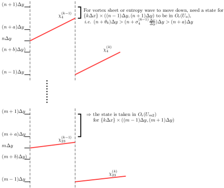
Figure 5. Separation of the initial data

We will establish a bound on the total variation of $U_{\Delta x,\theta}$ on the $k$-mesh curves to establish $C_{3}(k)$ and $C_{1}(k)$.

Definition 5.1.

A $k$-mesh curve is an unbounded piecewise linear curve consisting of line segments between the mesh points, lying in the strip:

$$(k-1)\Delta x\leq x\leq(k+1)\Delta x$$

with each line segment of form $P_{k-1,n-1}P_{k,n}$ or $P_{k,n}P_{k+1,n+1}$.

Clearly, for any $k>0$, each $k$-mesh curve $I$ divides plane $\mathbb{R}^{2}$ into a part $I^{+}$ and a part $I^{-}$, where $I^{-}$ is the one containing set $\{x<0\}$. As in [19], we partially order these mesh curves by saying $J>I$ if every point of $J$ is either on $I$ or contained in $I^{+}$, and we call $J$ an immediate successor to $I$ if $J>I$ and every mesh point of $J$, except one, is on $I$. We now define a Glimm-type functional on these mesh curves.

Definition 5.2.

Define

$$F_{s}(J) =C^{*}\sum_{j=1}^{4}|\sigma_{i}^{J}-\sigma_{i0}|+F(J)+KQ(J),$$

$$F(J) =L(J)+\tilde{K}_{43}|\alpha_{4s1}|+\tilde{K}_{12}|\alpha_{1s4}|,$$

$$L(J) =L^{1}(J)+L^{2}(J)+L^{3}(J)+L^{4}(J),$$

$$L^{j}(J) =\sum_{j=1}^{4}K^{*}_{ij}L_{i}^{j}(J),$$

$$L^{j}_{i}(J) =\sum\left\{|\alpha_{i}|\,:\,\alpha_{i}\text{ crosses }J\text{ in region }(j)\right\},$$

$$Q(J) =\sum\{|\alpha_{i}||\beta_{j}|\,:\,\text{ both }\alpha_{i}\text{ and }\beta_{j}\text{ cross }J\text{ and approach}\},$$

where $|\alpha_{4s1}|$ and $|\alpha_{1s4}|$ are the strengths of the weak $4$–shock and $1$–shock that emanate from the same point as the strong $1$–shock and $4$–shock, respectively, and these two weak waves are excluded from $L_{4}^{3}$ and $L_{1}^{2}$, respectively.

Remark 5.1.

$L(J)+C^{*}\sum_{j=1}^{4}|\sigma_{i}^{J}-\sigma_{i0}|$ measures the total variation of $\left.U\right|_{J}$, owing to Lemma 5.1; each term $L^{i}(J)$ measures the total variation in region $(i)$, and each term $|\sigma_{i}^{J}-\sigma_{i0}|$ measures the magnitude of jumps of $U$ between the regions separated by the large shocks. We also see that $Q(J)\leq L(J)$ for $L(J)$ small enough, so that $Q(J)$ is equivalent to $F_{s}(J)+C^{*}\sum_{j=1}^{4}|\sigma_{i}^{J}-\sigma_{i0}|$.

Proposition 5.1.

Suppose that $I$ and $J$ are two $k$–mesh curves such that $J$ is an immediate successor of $I$. Suppose that

$$\big{|}U_{\Delta x,\theta}|_{I\cap(\Omega^{(1)}_{\Delta x,k-1}\cup\Omega^{(1)}_{\Delta x,k})}-U_{b}\big{|}<\epsilon,\qquad\,\,\,\,\big{|}U_{\Delta x,\theta}|_{I\cap(\Omega^{(2)}_{\Delta x,k-1}\cup\Omega^{(2)}_{\Delta x,k})}-U_{m1}\big{|}<\epsilon,$$

$$\big{|}U_{\Delta x,\theta}|_{I\cap(\Omega^{(3)}_{\Delta x,k-1}\cup\Omega^{(3)}_{\Delta x,k})}-U_{m2}\big{|}<\epsilon,\qquad\big{|}U_{\Delta x,\theta}|_{I\cap(\Omega^{(4)}_{\Delta x,k-1}\cup\Omega^{(4)}_{\Delta x,k})}-U_{a}\big{|}<\epsilon,$$

$$|\sigma^{I}_{j}-\sigma_{j0}|<\hat{\epsilon}(\epsilon),\qquad j=1,2,3,4,$$

for some $\hat{\epsilon}(\epsilon)>0$ determined in Lemma 5.1. Then there exists $\tilde{\epsilon}>0$ such that, if $F_{s}(I)\leq\tilde{\epsilon}$,

$$F_{s}(J)\leq F_{s}(I),$$

and hence

$$\big{|}U_{\Delta x,\theta}|_{J\cap(\Omega^{(1)}_{\Delta x,k-1}\cup\Omega^{(1)}_{\Delta x,k})}-U_{b}\big{|}<\epsilon,\quad\,\,\,\,\big{|}U_{\Delta x,\theta}|_{J\cap(\Omega^{(2)}_{\Delta x,k-1}\cup\Omega^{(2)}_{\Delta x,k})}-U_{m1}\big{|}<\epsilon,$$

$$\big{|}U_{\Delta x,\theta}|_{J\cap(\Omega^{(3)}_{\Delta x,k-1}\cup\Omega^{(3)}_{\Delta x,k})}-U_{m2}\big{|}<\epsilon,\quad\big{|}U_{\Delta x,\theta}|_{J\cap(\Omega^{(4)}_{\Delta x,k-1}\cup\Omega^{(4)}_{\Delta x,k})}-U_{a}\big{|}<\epsilon,$$

$$|\sigma^{J}_{j}-\sigma_{j0}|<\hat{\epsilon}(\epsilon)\qquad\mbox{for $j=1,2,3,4$}.$$

Proof.

We make $M\geq 2$ larger to ensure that it is bigger than all the $O(1)$–terms in §4, and that $M\geq\frac{\Delta y}{\Delta x}$. With the fixed $M$ from here on, we now define our constants in terms of it. We set

$$\tilde{\epsilon}=\frac{1}{1024M^{3}}$$

and

$$K=16M,\qquad C^{*}=\frac{1}{128M^{2}},$$

$$K^{*}_{11}=K^{*}_{21}=K^{*}_{31}=K^{*}_{41}=K^{*}_{14}=K^{*}_{24}=K^{*}_{34}=K^{*}_{44}=1,$$

$$K^{*}_{12}=K^{*}_{43}=\frac{1}{M},\quad K^{*}_{13}=K^{*}_{42}=1+\frac{2}{M},$$

$$\tilde{K}^{*}_{42}=\tilde{K}^{*}_{13}=\frac{1}{16M},\quad K^{*}_{22}=K^{*}_{32}=K^{*}_{2,3}=K^{*}_{33}=\frac{1}{32M}.$$

Let $\Lambda$ be the diamond that is formed by $I$ and $J$. We can assume that $I=I_{0}\cup I^{\prime}$ and $J=J_{0}\cup J^{\prime}$ such that $\partial\Lambda=I^{\prime}\cup J^{\prime}$. We divide our proof into different cases, based on where diamond $\Lambda$ is located.

Case 1: Weak-weak interaction. Suppose that $\Lambda$ lies in the interior of a region $(i)$; see Figure 6. Then, by Proposition 4.1,

$$L^{i}(J)-L^{i}(I) \leq\sum_{j=1}^{4}K^{*}_{ij}MQ(\Lambda),$$

and

$$Q(J)-Q(I) =\Big{(}Q(I_{0})+\sum_{i=1}^{4}Q(\delta_{i},I_{0})\Big{)}-\Big{(}Q(I_{0})+Q(\Lambda)+\sum_{i=1}^{4}Q(\alpha_{i},I_{0})+\sum_{i=1}^{4}Q(\beta_{i},I_{0})\Big{)}$$

$$\leq\big{(}4ML(I_{0})-1\big{)}Q(\Lambda)$$

$$\leq-\frac{1}{2}Q(\Lambda),$$

when $L(I_{0})\leq\tilde{\epsilon}\leq\frac{1}{8M}$. Since $K_{ij}^{*}<2$ for all $i$ and $j$, we have

$$\sum_{j=1}^{4}K^{*}_{ij}M\leq 8M=\frac{K}{2},$$

so that $F_{s}(J)\leq F_{S}(I)$.

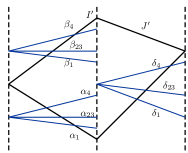
ing

Figure 6. Case 1: Weak wave interaction

Case 2: Weak waves interact with the strong vortex sheet/entropy wave from below. Suppose that the approximate strong vortex sheet/entropy wave enters $\Lambda$ from above; see Figure 7.

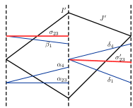
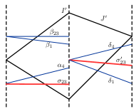
Figure 7. Cases 2 & 3: Weak waves interact with the strong vortex sheet/entropy wave from below and above

We have

$$L^{3}_{4}(J)-L^{3}_{4}(I) =|\delta_{4}|\leq M|\alpha_{4}|+M|\beta_{1}|(|\alpha_{2}|+|\alpha_{3}|),$$

$$L^{2}_{1}(J)-L_{1}^{2}(I) =|\delta_{1}|-|\beta_{1}|\leq|\alpha_{4}|+M|\beta_{1}|(+|\alpha_{2}|+|\alpha_{3}|),$$

$$L^{2}_{i}(J)-L^{2}_{i}(I) =-|\alpha_{i}|\qquad\mbox{for}\,\,i=2,3,$$

$$Q(J)-Q(I) =Q(I_{0})+Q(\delta_{4},I_{0})+Q(\delta_{1},I_{0})$$

$$\quad-\big{\{}Q(I_{0})+|\beta_{1}|(|\alpha_{2}|+|\alpha_{3}|)+Q(\beta_{1},I_{0})+Q(\beta_{4},I_{0})$$

$$\quad\quad\,\,\,+Q(\alpha_{1},I_{0})+Q(\alpha_{2},I_{0})+Q(\alpha_{3},I_{0})+Q(\alpha_{4},I_{0})\big{\}}$$

$$\leq(1+M)|\alpha_{4}|L(I_{0})+\big{(}ML(I_{0})-1\big{)}|\beta_{1}|\big{(}|\alpha_{1}|+|\alpha_{2}|+|\alpha_{3}|\big{)}$$

$$\leq 2M|\alpha_{4}|L(I_{0})-\frac{1}{2}|\beta_{1}|\big{(}|\alpha_{2}|+|\alpha_{3}|\big{)},$$

and

$$|\sigma_{i}^{J}-\sigma_{i}^{I}| \leq M|\alpha_{4}|+|\alpha_{i}|+M|\beta_{1}|\big{(}|\alpha_{2}|+|\alpha_{3}|\big{)}\qquad\mbox{for $i=2,3$}.$$

Then we obtain

$$F_{s}(J)-F_{s}(I)\leq\, \big{(}MK_{43}^{*}+K_{12}^{*}-K^{*}_{42}+2MKL(I_{0})+MC^{*}\big{)}|\alpha_{4}|$$

$$+\Big{(}MK_{43}^{*}+K_{12}^{*}+2MC^{*}-\frac{K}{2}\Big{)}|\beta_{1}|\big{(}|\alpha_{2}|+|\alpha_{3}|\big{)}$$

$$+(C^{*}-K^{*}_{22})|\alpha_{2}|+(C^{*}-K^{*}_{32})|\alpha_{3}|$$

$$\leq \,\Big{(}1+\frac{2}{M}-(1+\frac{2}{M})+\frac{1}{32M}+\frac{1}{128M}\Big{)}|\alpha_{4}|$$

$$+\sum_{i=1}^{3}\Big{(}1+\frac{1}{M}-8M\Big{)}|\beta_{1}|\big{(}|\alpha_{2}|+|\alpha_{3}|\big{)}\leq 0.$$

Case 3: Weak waves interact with the strong vortex sheet/entropy wave from above. Suppose that the approximate vortex sheet/entropy wave enters $\Lambda$ from below; see Figure 7. This case follows by symmetry from the above case, owing to the symmetry between Propositions 4.2 and 4.3, and the symmetry between the coefficients.

Case 4: Weak waves interact with the strong $1$–shock from above. Suppose that the strong $1$–shock enters $\Lambda$ from below; see Figure 8. By Proposition 4.4, we have

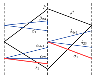
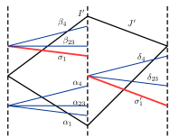
Figure 8. Cases 4 & 5: Weak waves interact with the strong $1$–shock from above and below

$$L_{i}^{2}(J)-L_{i}^{2}(I) =|\delta_{i}|-|\beta_{i}|-|\alpha_{i}|\leq M|\beta_{1}|+M|\alpha_{4}|(|\beta_{1}|+|\beta_{2}|+|\beta_{3}|)\qquad\mbox{for $i=2,3$},$$

$$L_{j}^{2}(J)-L_{j}^{2}(I) =-|\beta_{j}|\qquad\mbox{for $j=1,4$},$$

and

$$Q(J)-Q(I)= \,Q(I_{0})+Q(\delta_{2},I_{0})+Q(\delta_{3},I_{0})+Q(\delta_{4},I_{0})$$

$$-\big{\{}Q(I_{0})+Q(\alpha_{2},I_{0})+Q(\alpha_{3},I_{0})+Q(\alpha_{4},I_{0})$$

$$\,\,\quad+Q(\beta_{1},I_{0})+Q(\beta_{2},I_{0})+Q(\beta_{3},I_{0})+Q(\beta_{4},I_{0})$$

$$\,\,\quad+|\alpha_{4s1}|(|\beta_{1}|+|\beta_{2}|+|\beta_{3}|)+|\alpha_{3}|(|\beta_{1}|+|\beta_{2}|)+|\alpha_{2}||\beta_{1}|\big{\}}$$

$$\leq \,ML(I_{0})|\beta_{1}|+(ML(I_{0})-1)|\alpha_{4}|(|\beta_{1}|+|\beta_{2}|+|\beta_{3}|)$$

$$-|\alpha_{3}|(|\beta_{1}|+|\beta_{2}|)-|\alpha_{2}||\beta_{1}|$$

$$\leq \,ML(I_{0})|\beta_{1}|-\frac{1}{2}\big{(}\alpha_{4}|(|\beta_{1}|+|\beta_{2}|+|\beta_{3}|)+|\alpha_{3}|(|\beta_{1}|+|\beta_{2}|)+|\alpha_{2}||\beta_{1}|\big{)},$$

$$|\delta_{4s1}|-|\alpha_{4s1}| \leq M|\beta_{1}|+M|\alpha_{4}|(|\beta_{1}|+|\beta_{2}|+\beta_{3}|),$$

and

$$|\sigma^{J}_{1}-\sigma^{I}_{1}| \leq M|\beta_{1}|+M|\alpha_{4}|(|\beta_{1}|+|\beta_{2}|+|\beta_{3}|).$$

Therefore, we obtain

$$F_{s}(J)-F_{s}(I)\leq \,\big{(}M(K_{22}^{*}+K_{32}^{*}+\tilde{K}_{42}^{*})+KML(I_{0})+C^{*}M-K_{42}^{*}\big{)}|\beta_{1}|$$

$$+\big{(}-\frac{K}{2}+M(K_{22}^{*}+K_{32}^{*}+\tilde{K}_{42}^{*})+C^{*}M\big{)}|\alpha_{4}|(|\beta_{1}|+|\beta_{2}|+|\beta_{3}|)$$

$$\leq \,0.$$

Case 5: Weak waves interact with the strong $1$–shock from below. Suppose that the strong $1$–shock enters $\Lambda$ from above; see Figure 8. By Proposition 4.5, we have

$$L_{i}^{2}(J)-L_{i}^{2}(I)\leq M\big{(}|\alpha_{1}|+|\alpha_{2}|+|\alpha_{3}|+|\alpha_{4}\big{)}\qquad\mbox{for $i=2,3$},$$

$$L_{j}^{1}(J)-L_{j}^{1}(I)=-|\alpha_{j}|\qquad\mbox{for $j=1,2,3,4$},$$

$$|\delta_{4}|-|\beta_{4}|\leq M(|\alpha_{1}|+|\alpha_{2}|+|\alpha_{3}|+|\alpha_{4}),$$

$$|\sigma_{1}^{J}-\sigma_{1}^{I}|\leq M(|\alpha_{1}|+|\alpha_{2}|+|\alpha_{3}|+|\alpha_{4}),$$

$$Q(J)-Q(I)= \,Q(I_{0})+Q(\delta_{1},I_{0})+Q(\delta_{2},I_{0})+Q(\delta_{3},I_{0})+Q(\delta_{4},I_{0})$$

$$\,-\big{\{}Q(\alpha_{1},I_{0})+Q(\alpha_{2},I_{0})+Q(\alpha_{3},I_{0})+Q(\alpha_{4},I_{0})$$

$$\,\quad\,\,+Q(\beta_{2},I_{0})+Q(\beta_{3},I_{0})+Q(\beta_{4},I_{0})$$

$$\,\quad\,\,+|\alpha_{4}|(|\beta_{2}|+|\beta_{3}|+\mathbf{1}_{([0,\infty)^{2})^{c}}(\alpha_{4},\beta_{4})|\beta_{4}|)+|\alpha_{3}||\beta_{2}|\big{\}}$$

$$\leq \,ML(I_{0})(|\alpha_{1}|+|\alpha_{2}|+|\alpha_{3}|+|\alpha_{4}|)$$

$$\,-\big{(}|\alpha_{4}|(|\beta_{2}|+|\beta_{3}|+\mathbf{1}_{([0,\infty)^{2})^{c}}(\alpha_{4},\beta_{4})|\beta_{4}|)+|\alpha_{3}||\beta_{2}|\big{)}.$$

Then

$$F_{s}(J)-F_{s}(I)\leq \,\sum_{j=1}^{4}\left(M(K^{*}_{22}+K^{*}_{32}+\tilde{K}^{*}_{42})+KML(I_{0})+MC^{*}-K_{j1}\right)|\alpha_{j}|$$

$$\leq \,-\frac{1}{32}\sum_{j=1}^{4}|\alpha_{j}|\leq 0.$$

Case 6: Weak waves interact with the strong $4$–shock from below. Suppose that the strong $4$–shock enters $\Lambda$ from above; see Figure 9. By symmetry from Case 4, we conclude that $F_{s}(J)\leq F_{s}(I)$, due to the symmetry between Propositions 4.4 and 4.7.

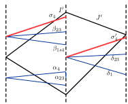
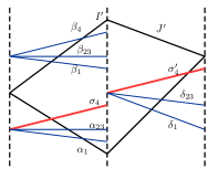
Figure 9. Cases 6 & 7: Weak waves interact with the strong $4$–shock from below and above.

Case 7: Weak waves interact with the strong $4$–shock from above. Suppose that the strong $4$–shock enters $\Lambda$ from below; see Figure 9. By symmetry from Case 5, we obtain that $F_{s}(J)\leq F_{s}(I)$, owing to the symmetry between Propositions 4.5 and 4.6. ∎

Let $I_{k}$ be the $k$–mesh curve lying in $\{(j-1)\Delta x\leq x\leq j\Delta x\}$. From Proposition 5.1, we obtain the following theorem for any $k\geq 1$:

Theorem 5.1.

Let $\tilde{\epsilon},\hat{\epsilon}(\epsilon),K$, and $C^{*}$ be the constants specified in Proposition 5.1. If the induction hypotheses $C_{1}(k-1)-C_{4}(k-1)$ hold and $F_{s}(I_{k-1})\leq\tilde{\epsilon}$, then

$$\big{|}U_{\Delta x,\theta}|_{\Omega^{(1)}_{\Delta x,k}}-U_{b}\big{|}<\epsilon,\qquad\,\,\,\,\big{|}U_{\Delta x,\theta}|_{\Omega^{(2)}_{\Delta x,k}}-U_{m1}\big{|}<\epsilon,$$

$$\big{|}U_{\Delta x,\theta}|_{\Omega^{(3)}_{\Delta x,k}}-U_{m2}\big{|}<\epsilon,\qquad\big{|}U_{\Delta x,\theta}\mid_{\Omega^{(4)}_{\Delta x,k}}-U_{a}\big{|}<\epsilon,$$

$$|\sigma^{(k)}_{j}-\sigma_{j0}|<\hat{\epsilon}(\epsilon)\qquad\mbox{for $j=1,2,3,4$},$$

and

$$F_{s}(I_{k})\leq F_{s}(I_{k-1}).$$ (5.1)

Moreover, we obtain the following theorem by the construction of our approximate solutions:

Theorem 5.2.

There exists $\epsilon>0$ such that, if

$$\mathrm{TV}\left(U_{0}(\cdot)-\overline{U}(0,\cdot)\right)<\epsilon,$$

then, for any $\theta\in\prod_{k=0}^{\infty}(-1,1)$ and every $\Delta x>0$, the modified Glimm scheme defines a family of strong approximate fronts $\chi_{j,\Delta x,\theta}$, $j=1,2,3,4$, in $\Omega_{\Delta x,\theta}$ which satisfy $C_{1}(k-1)-C_{4}(k-1)$ and (5.1). In addition,

$$\left\lvert\chi_{j,\Delta x,\theta}(x+h)-\chi_{j,\Delta x,\theta}(x)\right\rvert\leq\left(|\sigma_{j0}|+2M\right)|h|+2\Delta y$$

for any $x\geq 0$ and $h>0$.

5.3. Estimates on the Approximate Strong Fronts

Let

$$\sigma_{j,\Delta x,\theta}(x)=\sigma^{(k)}_{j}\qquad\text{for $x\in(k\Delta x,(k+1)\Delta x]$ and $j=1,2,3,4$},$$ (5.2)

$$s_{i,\Delta x,\theta}(x)=\sigma_{i,\Delta x,\theta}(x)\qquad\mbox{for $i=1,4$},$$ (5.3)

$$s_{2,3,\Delta x,\theta}=\left.\frac{v_{\Delta x,\theta}}{u_{\Delta x,\theta}}\right|_{\{y=\chi^{(k)}_{2,3}\}}\qquad\text{for $x\in(k\Delta x,(k+1)\Delta x]$}.$$ (5.4)

Then, by the estimates in Proposition 5.1, we have

Proposition 5.2.

There exists $\tilde{M}$, independent of $\Delta x,\theta$, and $U_{\Delta x,\theta}$, such that

$$TV\{\sigma_{j,\Delta x,\theta}\mid[0,\infty)\}=\sum_{k=0}^{\infty}|\sigma_{(k+1)}-\sigma_{(k)}|\leq\tilde{M}.$$

Proof.

We follow the proof in [11, pp. 290]. For any $k\geq 1$, and the interaction diamond $\Lambda\subset\{(k-1)\Delta x\leq x\leq(k+1)\Delta x\}$, define

$$E_{\Delta x,\theta}(\Lambda)=\begin{cases}0&\text{Case }1,\\ |\alpha_{2}|+|\alpha_{3}|+|\alpha_{4}|&\text{Case }2,\\ |\beta_{1}|+|\beta_{2}|+|\beta_{3}|&\text{Case }3,\\ |\beta_{1}|&\text{Case }4,\\ |\alpha_{1}|+|\alpha_{2}|+|\alpha_{3}|+|\alpha_{4}|&\text{Case }5,\\ |\alpha_{4}|&\text{Case }6,\\ |\beta_{1}|+|\beta_{2}|+|\beta_{3}|+|\beta_{4}|&\text{Case }7.\end{cases}$$ (5.5)

We see from Proposition 5.1 that

$$\sum_{\Lambda}E_{\Delta x,\theta}\leq\sum_{\Lambda}\frac{1}{\tilde{\epsilon}}\big{(}F_{s}(I)-F_{s}(J)\big{)}\leq\frac{1}{\tilde{\epsilon}}F_{s}(0)=M_{1}.$$

Since the quadratic terms from the interacting waves can always be dominated by $F_{S}(J)$, as shown in §4, we have

$$\sum_{k=0}^{\infty}|\sigma^{(k+1)}_{j}-\sigma^{(k)}_{j}|\leq M\sum_{\Lambda}E_{\Delta x,\theta}(\Lambda)\leq M_{1}:=\tilde{M}.$$

∎

Therefore, we also conclude the following:

Proposition 5.3.

There exists $\tilde{\tilde{M}}$, independent of $\Delta x,\theta$, and $U_{\Delta x,\theta}$, such that, for $j=1,2,3,4$,

$$\mathrm{TV}\{s_{j,\Delta x,\theta}(\cdot)\,\mid\,[0,\infty)\}\leq\tilde{\tilde{M}}.$$

Proof.

For $j=1,4$, this follows immediately from Proposition 5.2. For $j=2,3$, observe that, if we make $O_{\epsilon}(U_{m1})$ small enough so that $\frac{u_{m1}}{2}<u<2u_{m1}$ and $-1<v<1$ for any $U=(u,v,p,\rho)\in O_{\epsilon}(U_{m1})$, we have

$$\mathrm{TV}\{s_{j,\Delta x,\theta}(\cdot)\,\mid\,[0,\infty)\}\leq\frac{4}{u_{m2}^{2}}\big{(}2u_{m2}+1\big{)}\mathrm{TV}(U_{\Delta x,\theta})\leq C\,\mathrm{TV}(U_{0}).$$

∎

6. Global Entropy Solutions

In this section, we show the convergence of the approximate solutions to an entropy solution close to the four-wave configuration solution.

6.1. Convergence of the approximate solutions

Lemma 6.1.

For any $h>0$ and $x\geq 0$, there exists a constant $\check{N}$, independent of $\Delta x,\theta$, and $h$, such that

$$\int_{-\infty}^{\infty}\left\lvert U_{\Delta x,\theta}(x+h,y)-U_{\Delta x,\theta}(x,y)\right\rvert\,dy\leq\check{N}|h|.$$

Proof.

By Fubini’s theorem and Theorem 5.2,

$$\int_{-\infty}^{\infty}\left\lvert U_{\Delta x,\theta}(x+h,y)-U_{\Delta x,\theta(x,y)}\right\rvert\,dy \leq\int_{-\infty}^{\infty}\int_{x}^{x+h}|d(U_{\Delta x,\theta}(s,y))|\,dy$$

$$=\int_{x}^{x+h}\mathrm{TV}(U_{\Delta x,\theta}(s,\cdot))\,ds$$

$$\leq\check{N}|h|\mathrm{TV}(U_{0}).$$

∎

Since $U_{\Delta x,\theta}$ is an entropy solution in each square $T_{k,n},k+n\equiv 0\,(\mathrm{mod}\,2)$, we see that, for each test function $\phi\in C^{\infty}_{0}(\mathbb{R}^{2};\mathbb{R}^{4})$,

$$\int_{k\Delta x}^{(k+1)\Delta x}\int^{(n+1)\Delta y}_{(n-1)\Delta y}\big{(}\partial_{x}\phi\cdot H(U_{\Delta x,\theta})+\partial_{y}\phi\cdot W(U_{\Delta x,\theta})\big{)}\,dy\,dx$$

$$=\int_{k\Delta x}^{(k+1)\Delta x}\big{(}\phi(x,(n+1)\Delta y)\cdot W(U_{\Delta x,\theta}(x,(n+1)\Delta y))$$

$$\qquad\qquad\qquad-\phi(x,(n-1)\Delta y)\cdot W(U_{\Delta x,\theta}(x,(n-1)\Delta y))\big{)}\,dx$$

$$\quad+\int_{(n-1)\Delta y}^{(n+1)\Delta y}\big{(}\phi((k+1)\Delta x,y)\cdot H(U_{\Delta x,\theta}((k+1)\Delta x-,y))$$

$$\qquad\qquad\qquad\,\,\,\,\,-\phi(k\Delta x,y)\cdot H(U_{\Delta x,\theta}(k\Delta x+,y))\big{)}\,dx.$$

Then, summing over all $k$ and $n$ with $k+n\equiv 1\,(\mathrm{mod}\,2)$ and re-arranging the terms, we have

$$\int_{0}^{\infty}\int^{\infty}_{-\infty}\big{(}\partial_{x}\phi\cdot H(U_{\Delta x,\theta})+\partial_{y}\phi\cdot W(U_{\Delta x,\theta})\big{)}\,dy\,dx$$

$$=\sum_{k=1}^{\infty}\int_{0}^{\infty}\phi(k\Delta x,y)\cdot\big{(}H(U_{\Delta x,\theta}(k\Delta x-,y))-H(U_{\Delta x,\theta}(k\Delta x+,y))\big{)}\,dx$$

$$\quad-\int_{-\infty}^{\infty}\phi(0,y)\cdot H(U_{\Delta x,\theta}(0+,y))\,dy.$$

Denote

$$J(\theta,\Delta x,\phi)=\sum_{k=1}^{\infty}\int_{-\infty}^{\infty}\phi(k\Delta x,y)\cdot\big{(}H(U_{\Delta x,\theta}(k\Delta x+,y))-H(U_{\Delta x,\theta}(k\Delta x-,y))\big{)}\,dy.$$

Following the same steps as in [23, Chapter 19], we have

Lemma 6.2.

There exist a null set $\mathcal{N}\subset\prod_{k=0}^{\infty}(-1,1)$ and a subsequence $\{\Delta x_{j}\}_{j=1}^{\infty}\subset\{\Delta x\}$, which tends to 0, such that

$$J(\theta,\Delta x_{j},\phi)\rightarrow 0\,\,\qquad\text{when }\Delta x_{j}\rightarrow 0$$

for any $\theta\in\prod_{k=0}^{\infty}(-1,1)\setminus\mathcal{N}$ and $\phi\in C^{\infty}_{0}(\mathbb{R}^{2};\mathbb{R}^{4})$.

To complete the proof of the main theorem, we need to estimate the slope of the approximate strong fronts. For $k\geq 1$, $i=1,2,3,4$,

$$d^{i}_{k}=s_{i}^{(k-1)}\frac{\Delta x}{\Delta y},$$

with $d_{k}^{2,3}:=d^{2}_{k}=d^{3}_{k}$. Then, by the choice of $\frac{\Delta y}{\Delta x}$, we find that $d_{k}^{i}\in(-1,1)$, which depends only on $\{\theta_{l}\}_{l=1}^{k-1}$. We then define

$$I^{i}(x,\Delta x,\theta)=\sum_{k=0}^{\left[x/\Delta x\right]}I^{i}_{k}(\Delta x,\theta),$$

where

$$I^{i}_{k}(\Delta x,\theta)=\mathbf{1}_{(-1,d^{i}_{k})}(\theta_{k})(1-d^{i}_{k})\Delta y-\mathbf{1}_{(d^{i}_{k},1)}(\theta_{k})(1+d^{i}_{k})\Delta y\qquad\mbox{for $k\geq 1$},$$

and

$$I^{1}_{0}(\Delta x,\theta)=-4\Delta y,\quad I^{2}_{0}(\Delta x,\theta)=I^{3}_{0}(\Delta x,\theta)=0,\quad I^{4}_{0}(\Delta x,\theta)=4\Delta y.$$

Then $I^{i}_{k}(\Delta x,\theta)$ is the jump of $y=\chi_{i}(x)$ at $x=k\Delta x$, and is a measurable function of $(\Delta x,\theta)$, depending only on $U_{\Delta x,\theta}\mid_{\{0\leq x\leq k\Delta x\}}$ and $\{\theta_{l}\}_{l=0}^{k}$.

Lemma 6.3.

The following statements hold:

1. For any $x\geq 0$, $\Delta x\geq 0$, $\theta\in\prod_{k=0}^{\infty}(-1,1)$, and $i=1,2,3,4$,

   $$\chi_{i,\Delta x,\theta}=I^{i}(x,\Delta x,\theta)+\int_{0}^{x}s_{i,\Delta x,\theta}(s)\,ds;$$

2. There exist a null set $\mathcal{N}_{1}$ and a subsequence $\{\Delta_{l}\}_{l=1}^{\infty}\subset\{\Delta x_{j}\}_{j=1}^{\infty}$ such that

   $$\int_{0}^{\infty}e^{-x}|I(x,\Delta_{l},\theta)|^{2}\,dx\rightarrow 0\,\,\qquad\text{when }\Delta_{l}\rightarrow 0$$

   for any $\theta\in\prod_{k=0}^{\infty}(-1,1)\setminus\mathcal{N}_{1}$.

Proof.

The first part is a direct calculation. The second follows by the same proof as [11, pp. 292]; just take two sub-sub-sequences to obtain all three strong front slopes to converge. ∎

Theorem 6.1 (Existence and Stability).

There exist $\epsilon>0$ and $C>0$ such that, if the hypotheses of the main theorem hold, then, for each $\theta\in\prod_{k=1}^{\infty}(-1,1)\setminus(\mathcal{N}\cup\mathcal{N}_{1})$, there exists a sequence $\{\Delta_{l}\}_{l=1}^{\infty}$ of mesh sizes with $\Delta_{l}\rightarrow 0$ as $l\rightarrow\infty$, and functions $U_{\theta}\in BV(\mathbb{R}^{2}_{+};\mathbb{R}^{4})$ and $\chi_{j,\theta}\in\mathrm{Lip}(\mathbb{R}_{+};\mathbb{R})$ with $\chi_{j,\theta}(0)=0$, $j=1,2,3,4$, such that

1. $U_{\Delta l,\theta}$ converges to $U_{\theta}$ a.e. in $\mathbb{R}^{2}_{+}$, and $U_{\theta}$ is a global entropy solution of system (1.1) and satisfies the initial data (2.1) a.e.;

2. $\chi_{j,\Delta l,\theta}$ converges to $\chi_{j,\theta}$ uniformly in any bounded $x$-interval;

3. $s_{j,\Delta l,\theta}$ converges to $s_{j,\theta}\in BV([0,\infty))$ a.e. and

   $$\chi_{j,\theta}(x)=\int_{0}^{x}s_{j,\theta}(t)\,dt.$$

Proof.

Result (i) follows by the same steps as [23, Chapter 19], (ii) follows by Theorem 5.2 and the Arzela-Ascoli theorem, while (iii) follows Proposition 5.3 and the basic properties of BV functions. ∎

Acknowledgements.   The research of Gui-Qiang G. Chen was supported in part by the UK Engineering and Physical Sciences Research Council Award EP/E035027/1 and EP/L015811/1. The research of Matthew Rigby was supported in part by the UK Engineering and Physical Sciences Research Council Award EP/E035027/1.

References

- [1] M. Artola and A. Majda. Nonlinear development of instability in supersonic vortex sheets, I: The basic kink modes, Phys. D. 28: 253–281, 1987.
- [2] M. Artola and A. Majda. Nonlinear development of instability in supersonic vortex sheets, II: Resonant interaction among kink modes, SIAM J. Appl. Math. 49: 1310–1349, 1989.
- [3] A. Bressan. Hyperbolic Systems of Conservation Laws: The One-dimensional Cauchy Problem. Oxford University Press: Oxford, 2000.
- [4] T. Chang and L. Hsiao. The Riemann Problem and Interaction of Waves in Gas Dynamics. Longman Scientific & Technical, Essex: England, 1989.
- [5] G.-Q. Chen, Supersonic flow onto solid wedges, multidimensional shock waves and free boundary problems, Sci. China Math. 60: 1353–1370, 2017.
- [6] G.-Q. Chen, Convergence of the Lax-Friedrichs scheme for the system of equations of isentropic gas dynamics. III. Acta Math. Sci. (Chinese) 8:243 C276, 1988; Acta Math. Sci. (English Ed.) 6:75–120, 1986.
- [7] G.-Q. Chen and M. Feldman. The Mathematics of Shock Reflection-Diffraction and Von Neumann’s Conjecture. Annals of Mathematics Studies, 197, Princeton University Press: Princetion, 2018.
- [8] G.-Q. Chen, J. Kuang, and Y. Zhang, Two-dimensional steady supersonic exothermically reacting Euler flow past Lipschitz bending walls, SIAM J. Math. Anal. 49: 818–873, 2017.
- [9] G.-Q. Chen and T.-H. Li. Well-posedness for two-dimensional steady supersonic Euler flows past a Lipschitz wedge, J. Diff. Eqs. 244: 1521–1550, 2008.
- [10] G.-Q. Chen and Y.-G. Wang. Characteristic discontinuities and free boundary problems for hyperbolic conservation laws, In: Nonlinear Partial Differential Equations, The Abel Symposium 2010, Chapter 5, pp. 53–82, H. Holden and K. H. Karlsen (Eds.), Springer-Verlag: Heidelberg, 2012.
- [11] G.-Q. Chen, Y. Zhang, and D. Zhu. Existence and stability of supersonic Euler flows past Lipschitz wedges. Arch. Ration. Mech. Anal. 181(2):261–310, 2006.
- [12] G.-Q. Chen, Y. Zhang, and D. Zhu. Stability of compressible vortex sheets in steady supersonic Euler flows over Lipschitz walls. SIAM J. Math. Anal. 38(5):1660–1693 (electronic), 2006/07.
- [13] S.-X. Chen. Stability of a Mach configuration. Comm. Pure Appl. Math. 59(1):1–35, 2006.
- [14] S.-X. Chen. E-H type Mach configuration and its stability. Comm. Math. Phys. 315(3):563–602, 2012.
- [15] C. M. Dafermos. Hyperbolic Conservation Laws in Continuum Physics, 4th Edition, Springer-Verlag: Berlin, 2016.
- [16] X. Ding, Theory of conservation laws in China. In: Hyperbolic Problems: Theory, Numerics, Applications (Stony Brook, NY, 1994), pp. 110–119, World Sci. Publ., River Edge, NJ, 1996.
- [17] X. Ding (Ding Shia Shi), T. Chang (Chang Tung), J.-H. Wang (Wang Ching-Hua), L. Xiao (Hsiao Ling), and C.-Z. Zhong (Li Tsai-Chung). A study of the global solutions for quasi-linear hyperbolic systems of conservation laws. Sci. Sinica, 16: 317–335, 1973.
- [18] X. Ding, G.-Q. Chen, and P. Luo. Convergence of the Lax-Friedrichs scheme for the system of equations of isentropic gas dynamics. I. Acta Math. Sci. (Chinese) 7: 467–480, 1987; Acta Math. Sci. (English Ed.) 5: 415–432, 1985. II. Acta Math. Sci. (Chinese) 8: 61–94, 1988; Acta Math. Sci. (English Ed.) 5: 433–472, 1985.
- [19] J. Glimm. Solutions in the large for nonlinear hyperbolic systems of equations. Comm. Pure Appl. Math. 18:697–715, 1965.
- [20] P. D. Lax. Hyperbolic Systems of Conservation Laws and the Mathematical Theory of Shock Waves. SIAM-CBMS: Philadelphia, 1973.
- [21] M. Lewicka and K. Trivisa. On the well posedness of systems of conservation laws near solutions containing two large shocks. J. Diff. Eqs. 179(1):133–177, 2002.
- [22] T.-P. Liu, Large-time behaviour of initial and initial-boundary value problems of a general system of hyperbolic conservation laws. Comm. Math. Phys. 55:163–177, 1977.
- [23] J. Smoller. Shock Waves and Reaction-Diffusion Equations, Springer-Verlag: New York, 1994.