Large deviations conditioned on large deviations I: Markov chain and Langevin equation.

Abstract

We present a systematic analysis of stochastic processes conditioned on an empirical measure $Q_{T}$ defined in a time interval $[0,T]$ for large $T$. We build our analysis starting from a discrete time Markov chain. Results for a continuous time Markov process and Langevin dynamics are derived as limiting cases. We show how conditioning on a value of $Q_{T}$ modifies the dynamics. For a Langevin dynamics with weak noise, we introduce conditioned large deviations functions and calculate them using either a WKB method or a variational formulation. This allows us, in particular, to calculate the typical trajectory and the fluctuations around this optimal trajectory when conditioned on a certain value of $Q_{T}$.

1 Introduction

Understanding the frequency of rare events and the dynamical trajectories which generate them has become an important field of research in many physical situations including protein folding Mey2014 , chemical reactions Delarue2017 ; Dykman1994 , atmospheric activities Laurie2015 , glassy systems Garrahan2007 ; Garrahan2009 , disordered media Dorlas2001 , etc.. From the mathematical point of view, the statistical properties of rare events are characterized by large deviations functions dembo2009 ; Varadhan1966 ; Varadhan2003 ; Donsker19752 ; Hollander2008 ; TOUCHETTE2009 ; ellis1985 ; Derrida2007 ; Hurtado2014 . In physics, a particular interest for large deviations functions arose in the context of non-equilibrium statistical physics from the discovery of the fluctuation theorem Kurchan1998 ; Gallavotti1995 ; Lebowitz1999 where the rare event consists in observing an atypical value of a current over a long time window. They also had been used for a long time to study stochastic dynamical systems in a weak noise limit Freidlin2012 ; Graham1985 ; Graham1973 or extended systems when the system size becomes large Bertini2014 ; Derrida2007 ; Bertini2001 .

One of the simplest questions one may ask about the large deviations functions is to consider an empirical measure $Q_{T}$ of the form

$$Q_{T}=\int_{0}^{T}dt\,f({C}_{t})$$ (1)

where $f({C}_{t})$ is a function of the configuration ${C}_{t}$ of a stochastic (or a chaotic) system at time $t$ and to try to determine the probability that this empirical measure takes any atypical value $q\,T$. For large $T$, the large deviations function $\phi(q)$ is then simply defined by Varadhan1984 ; Donsker19752 ; Maes2008 ; Maes20082 ; Bodineau2004 ; Derrida2007 ; Bertini2005Current ; Hurtado2014 ; Hurtado2010

$$\textrm{ Prob}(Q_{T}=qT)\sim e^{-T\,\phi(q)}\qquad\textrm{for large }T$$ (2)

(Here the precise meaning of the symbol $\sim$ is that $\lim_{T\rightarrow\infty}\frac{1}{T}\log\textrm{Prob}(qT)=-\phi(q)$, and this will be used throughout this article.) A rather common situation is when $\phi(q)$ vanishes at a single value $q^{*}$ of $q$ (the most likely value of $q$) and where $\phi(q)>0$ for $q\neq q^{*}$. The main question we try to address in the present paper is what are the dominant trajectories of a stochastic process which contribute to this large deviations function and how to describe their effective dynamics. In particular, we want to understand how to predict the probability $P_{t}({C}|Q_{T}=q\,T)$ of finding the system in a configuration ${C}$ at an arbitrary time $t$, conditioned on a certain value of $Q_{T}$.

A very related approach Jack2010 ; Jack2015 ; Chetrite2013 ; Chetrite2015 ; TOUCHETTE2017 ; Maes2008 ; Maes20082 ; Lecomte20072 ; Hartmann2012 ; Bertini2015 (what we will call the canonical approach) consists in weighting all the events by an exponential of $Q_{T}$ and to try to determine the probability

$$P_{t}^{(\lambda)}(C)=\frac{\int dQ\,e^{\lambda Q}P_{t}(C,Q)}{\sum_{C^{\prime}}\int dQ\,e^{\lambda Q}P_{t}(C^{\prime},Q)}$$ (3)

where $P_{t}(C,Q)$ is the joint probability of configuration $C$ at time $t$ and the observable $Q_{T}$ to take value $Q$ given the system in its steady state. This is in contrast to the previous case (where $Q_{T}$ was fixed and that we call the microcanincal case). As we shall see (in particular, in Section 2 and Appendix A) these canonical and microcanonical ensembles are related in the usual way in the large $T$ limit (which plays here the same role as the thermodynamic limit in standard statistical mechanics).

Our paper will start by reviewing and extending some known aspects of the large deviations function for Markov processes and for the Langevin equation (see Section 2 and Section 3). In the large $T$ limit, one has to distinguish five regions (see Figure 1) for which we calculate how the measure and the dynamics are modified by the conditioning on $Q_{T}$. Then, we will consider the Langevin equation in the weak noise limit, first using a Wentzel-Kramers-Brillouin (WKB) approach Landau (Section 4) and a variational approach (Section 6) based on the search of an optimal path which minimizes an action. This will allow in particular to obtain the equation followed by the optimal trajectory under conditioning. Lastly we will see in Section 7 that the effect of conditioning is to break causality in the sense that a trajectory becomes correlated to the noise in the future.

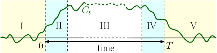
Figure 1: A schematic of a time evolution of a Markov process $C_{t}$ when conditioned on an empirical observable $Q_{T}$ measured in a large time interval $[0,T]$. Different regions denote different parts of the evolution: (I) $t<0$, (II) $t\geq 0$ but small, (III) $t$ and $T-t$ both large, (IV) $T-t>0$ but small, and (V) $t\geq T$.

2 Markov Process

For large $T$, a schematic time evolution of a Markovian stochastic system conditioned to take a certain value of $Q_{T}$ is shown in Figure 1 where one has to consider five regions. The system starts from a typical configuration far in the past, and evolves to a quasi-stationary regime (region III in Figure 1), and finally relaxes to the typical state of the unconditioned dynamics. One knows Jack2010 ; Jack2015 ; Chetrite2013 ; Chetrite2015 ; TOUCHETTE2017 ; Lecomte20072 ; Garrahan2007 ; Garrahan2009 ; Evans2004 how to describe the effective dynamics in the quasi-stationary regime. For a Markov chain, the effective dynamics in region III is known to remain Markovian with transition rate which can be expressed in terms of the largest eigenvalue and eigenvectors of the tilted Markov matrix. This connection between conditioned dynamics and a biased ensemble appeared earlier in many contexts: Doob’s h-transformation Stroock , Donsker-Varadhan theory of large deviations Donsker19752 , rare events problems Jack2015 ; Chetrite2013 ; Chetrite2015 ; TOUCHETTE2017 ; Maes2008 ; Maes20082 ; Hartmann2012 ; Lecomte20072 ; Hirschberg2015 ; Schutz2016 ; Popkov2011 ; Popkov2010 ; Evans2004 , kinetically constrained models Garrahan2007 ; Garrahan2009 , optimal control theory Fleming1992 ; Chetrite20152 , and even in Quantum systems Carollo2018 . In this section, we give a simple derivation of the effective dynamics which extends to the five regions of Figure 1, the earlier results known in the quasi-stationary regime.

2.1 The tilted matrix

We focus here our discussion on a discrete time irreducible Markov process on a finite set of configurations. This Markov process is specified by the probability $M_{0}(C^{\prime},C)$ that the system jumps from configuration $C$ to $C^{\prime}$ in one time step. As we will see later, the continuous time Markov process and the Langevin dynamics can be obtained as limiting cases.

For this discrete time Markov process, we want to condition on a general empirical measure

$$Q_{T}=\sum_{t=0}^{T-1}f({\cal C}_{t})+\sum_{t=0}^{T-1}g({\cal C}_{t+1},{\cal C}_{t})$$ (4)

where $f$ and $g$ are arbitrary functions of the configurations. For example, by choosing $f(C)=\delta_{C,C_{a}}$ and $g(C^{\prime},C)=0$, the observable $Q_{T}$ represents the total time spent in a particular configuration $C_{a}$. Another choice $f(C)=0$ and $g(C^{\prime},C)=\delta_{C^{\prime},C_{b}}\delta_{C,C_{a}}$ would count the total number of jumps from configuration $C_{a}$ to configuration $C_{b}$.

Our goal is to describe the dynamics conditioned on a certain value of $Q_{T}$ for large $T$. In particular, we want to know what is the conditional probability $\mathcal{P}_{t}(C|Q_{T})$ for the system to be in a configuration $C$ at an arbitrary time $t$ when conditioned on the observable $Q_{T}$ defined by (4).

Let us first analyze the special case $t=T$. If we define the joint probability $P_{T}(C,Q|C_{0})$ for the system to be in a configuration $C$ at time $T$ and that the observable $Q_{T}$ defined by (4) takes value $Q$ given its initial configuration $C_{0}$ at time $0$, it satisfies a recursion relation:

$$P_{T}(C,Q|C_{0})=\sum_{C^{\prime}}M_{0}(C,C^{\prime})P_{T-1}(C^{\prime},Q-f(C^{\prime})-g(C,C^{\prime})|C_{0})$$ (5)

Then, it is easy to see that the generating function defined by

$$G_{T}^{(\lambda)}(C|C_{0})=\int dQ\;e^{\lambda Q}P_{T}(C,Q|C_{0})$$ (6)

satisfies

$$G_{T}^{(\lambda)}(C|C_{0})=\sum_{C^{\prime}}M_{\lambda}(C,C^{\prime})G_{T-1}^{(\lambda)}(C^{\prime}|C_{0})$$ (7)

where

$$M_{\lambda}(C,C^{\prime})=M_{0}(C,C^{\prime})e^{\lambda\left[f(C^{\prime})+g(C,C^{\prime})\right]}$$ (8)

is the tilted matrix Lebowitz1999 ; Derrida2007 ; Chetrite2013 ; Lecomte20072 ; Garrahan2009 ; Roche2004 ; Hirschberg2015 ; Popkov2010 ; Bertini2015 . Therefore, $G_{T}^{(\lambda)}(C|C_{0})=M_{\lambda}^{T}(C,C_{0})$ is the $(C,C_{0})$th element of the matrix $(M_{\lambda})^{T}$. For large $T$, the matrix elements of $(M_{\lambda})^{T}$ are dominated by the largest eigenvalue $e^{\mu(\lambda)}$ of $M_{\lambda}$, resulting in

$$G_{T}^{(\lambda)}(C|C_{0})\simeq e^{T\mu(\lambda)}R_{\lambda}(C)L_{\lambda}(C_{0})$$ (9)

where $R_{\lambda}(C)$ and $L_{\lambda}(C)$ are the associated right and left eigenvectors, respectively. For the prefactor in (9) to be correct the eigenvectors must be normalized with $\sum_{C}R_{\lambda}(C)L_{\lambda}(C)=1$.

• 1. It follows from (6, 9) that the cumulants of $Q_{T}$, for large $T$, can be obtained from the derivatives of $\mu(\lambda)$ at $\lambda=0$, and that $\lim_{T\rightarrow\infty}\frac{1}{T}\log\langle e^{\lambda Q_{T}}\rangle=\mu(\lambda)$.

  2. The Perron-Frobenius theorem VANKAMPEN2007193 ensures that the largest eigenvalue of $M_{\lambda}$ is positive and non-degenerate, and all components of the associated right and left eigenvectors are positive. For non-zero $\lambda$, the tilted matrix $M_{\lambda}$ is, in general, not Markovian (because $\sum_{C^{\prime}}M_{\lambda}(C^{\prime},C)\neq 1$) and non-Hermitian.

  3. In the case $\lambda=0$, the largest eigenvalue is $1$, with $L_{0}(C)=1$, and $R_{0}(C)$ is the steady state probability distribution of the Markov process $M_{0}$.

2.2 Ensemble equivalence

From (6) and (9), one can see by a saddle point calculation that for large $T$

$$P_{T}(C,Q=qT|C_{0})\simeq e^{-T\phi(q)}\sqrt{\frac{\phi^{\prime\prime}(q)}{2\pi T}}R_{\phi^{\prime}(q)}(C)L_{\phi^{\prime}(q)}(C_{0})$$ (10)

where the large deviation function $\phi(q)$ and the eigenvalue $e^{\mu(\lambda)}$ of the matrix $M_{\lambda}$ are related by a Legendre transformation

$$\mu(\lambda)=\lambda q-\phi(q)\qquad\mbox{with }\qquad\lambda=\phi^{\prime}(q)$$ (11)

We see from (10) that, for large $T$, the conditional distribution of $C$ at the final time is given by

$$\mathcal{P}_{T}(C|Q=qT)=\frac{P_{T}(C,Q=qT|C_{0})}{\sum_{C^{\prime}}P_{T}(C^{\prime},Q=qT|C_{0})}\simeq\frac{R_{\phi^{\prime}(q)}(C)}{\sum_{C^{\prime}}R_{\phi^{\prime}(q)}(C^{\prime})}$$ (12)

This shows that the initial condition $C_{0}$ is forgotten at large $T$. Therefore, we leave out the reference to $C_{0}$ in our notation for the conditional probability. On the other hand, in the $\lambda$-ensemble, using (9) one has the probability at the final time

$$P_{T}^{(\lambda)}(C)=\frac{G_{T}^{(\lambda)}(C|C_{0})}{\sum_{C^{\prime}}G_{T}^{(\lambda)}(C^{\prime}|C_{0})}\simeq\frac{R_{\lambda}(C)}{\sum_{C^{\prime}}R_{\lambda}(C^{\prime})}$$ (13)

Comparing (12) and (13) we see that the conditional probability $\mathcal{P}_{t=T}(C|Q=qT)$ for large $T$ can be obtained from the probability $P_{T}^{(\lambda)}(C)$ by substituting $\lambda=\phi^{\prime}(q)$. This shows that, for large $T$, the two ensembles are equivalent: fixing the value of $Q_{T}$ or weighting the events by a factor $e^{\lambda Q_{T}}$ lead to the same distribution of the final configuration $C$. The former is an analogue of the micro-canonical ensemble with fixed $Q_{T}$ and the latter is its canonical counterpart defined by the conjugate variable $\lambda$.

• For an irreducible Markov process on a finite configuration space, the spectral gap between the largest and the second largest eigenvalues is non-zero. Moreover, the functions $\phi(q)$ and $\mu(\lambda)$ are analytic and convex, and the equivalence (11) is assured. This may not be the case for systems with infinite configurations, where the gap may disappear and large deviations functions could become non-analytic Bodineau2005 ; Lecomte20072 ; Garrahan2007 ; Garrahan2009 ; Jack2010 ; Baek2017 ; Espigares2013 .

2.3 The measure conditioned on $Q_{T}$

As shown in Appendix A, the equivalence of ensembles holds not only at time $t=T$, but at any time $t$, as long as $T$ is large Jack2010 ; Jack2015 ; Chetrite2013 ; Chetrite2015 ; TOUCHETTE2017 . This states that, by generalizing (13), if we define the canonical probability

$$P_{t}^{(\lambda)}(C)=\frac{\int dQ\,e^{\lambda Q}P_{t}(C,Q)}{\sum_{C^{\prime}}\int dQ\,e^{\lambda Q}P_{t}(C^{\prime},Q)}$$ (14)

for any time $t$, then for large $T$,

$$\mathcal{P}_{t}(C|Q_{T}=qT)\simeq P_{t}^{(\lambda)}(C)\qquad\mbox{with}\qquad\lambda=\phi^{\prime}(q)$$ (15)

where $P_{t}(C,Q)$ is the joint probability of configuration $C$ at time $t$ and the observable $Q_{T}$ to take value $Q$ given the system in its steady state; $\mathcal{P}_{t}(C|Q)$ is the corresponding conditional probability.

This conditioned measure (14) for large $T$ takes different expressions in the five regions indicated in Figure 1. (A derivation is presented in Appendix A for region II and can be easily extended for other regions.)

• Region I. $t<0$

  $$P_{t}^{(\lambda)}(C)=\frac{\sum_{C^{\prime}}L_{\lambda}(C^{\prime})M_{0}^{-t}(C^{\prime},C)R_{0}(C)}{\sum_{C^{\prime}}L_{\lambda}(C^{\prime})R_{0}(C^{\prime})}$$ (16a)

• Region II. $0\leq t\ll T$

  $$P_{t}^{(\lambda)}(C)=\frac{\sum_{C^{\prime}}L_{\lambda}(C)M_{\lambda}^{t}(C,C^{\prime})R_{0}(C^{\prime})}{e^{t\mu(\lambda)}\sum_{C^{\prime}}L_{\lambda}(C^{\prime})R_{0}(C^{\prime})}$$ (16b)

• Region III. $1\ll t$ and $T-t\gg 1$

  $$P_{t}^{(\lambda)}(C)=R_{\lambda}(C)L_{\lambda}(C)$$ (16c)

• Region IV. $1\ll t<T$, i.e. $T-t=\mathcal{O}(1)$

  $$P_{t}^{(\lambda)}(C)=\frac{\sum_{C^{\prime}}M_{\lambda}^{T-t}(C^{\prime},C)R_{\lambda}(C)}{e^{(T-t)\mu(\lambda)}\sum_{C^{\prime}}R_{\lambda}(C^{\prime})}$$ (16d)

• Region V. $T\leq t$

  $$P_{t}^{(\lambda)}(C)=\frac{\sum_{C^{\prime}}M_{0}^{t-T}(C,C^{\prime})R_{\lambda}(C^{\prime})}{\sum_{C^{\prime}}R_{\lambda}(C^{\prime})}$$ (16e)

To be consistent with the notation of Section 2.1 we denote by $R_{0}(C)$ the steady state measure of the Markov process $M_{0}$. Therefore (13) is a special case of (16d). Another special case

$$P_{t=0}^{(\lambda)}(C)=\frac{L_{\lambda}(C)R_{0}(C)}{\sum_{C^{\prime}}L_{\lambda}(C^{\prime})R_{0}(C^{\prime})}$$ (17)

2.4 Time evolution of the conditioned process

Again by a straightforward generalization of the reasoning (see Appendix A), one can show that the equivalence of ensembles holds for the conditioned dynamics as well. In fact, the conditioned dynamics is itself a Markov process Jack2010 ; Jack2015 ; Chetrite2013 ; Chetrite2015 ; TOUCHETTE2017 . For this process, the probability of jump $W_{t}^{(\lambda)}(C^{\prime},C)$ from configuration $C$ at $t$ to $C^{\prime}$ at $t+1$ in the canonical ensemble (events weighted by $e^{\lambda Q_{T}}$) depends, in general, on time $t$. For example, for $t<0$,

$$W_{t}^{(\lambda)}(C^{\prime},C)={\sum_{C^{\prime\prime\prime},C^{\prime\prime}}M_{\lambda}^{T}(C^{\prime\prime\prime},C^{\prime\prime})\ M_{0}^{-t-1}(C^{\prime\prime},C^{\prime})\ M_{0}(C^{\prime},C)R_{0}(C)\over\sum_{C^{\prime\prime\prime},C^{\prime\prime}}M_{\lambda}^{T}(C^{\prime\prime\prime},C^{\prime\prime})\ M_{0}^{-t}(C^{\prime\prime},C)R_{0}(C)}$$

while for $0\leq t<T$,

$$W_{t}^{(\lambda)}(C^{\prime},C)=\frac{\sum_{C^{\prime\prime},C_{0}}M_{\lambda}^{T-t-1}(C^{\prime\prime},C^{\prime})M_{\lambda}(C^{\prime},C)M_{\lambda}^{t}(C,C_{0})R_{0}(C_{0})}{\sum_{C^{\prime\prime},C_{0}}M_{\lambda}^{T-t}(C^{\prime\prime},C)M_{\lambda}^{t}(C,C_{0})R_{0}(C_{0})}$$

For large $T$, the dominant contribution comes from the largest eigenvalue of $M_{\lambda}$, and one gets in the five regions of Figure 1:

• Region I.

  $$W_{t}^{(\lambda)}(C^{\prime},C)={\sum_{C^{\prime\prime}}L_{\lambda}(C^{\prime\prime})\ M_{0}^{-t-1}(C^{\prime\prime},C^{\prime})\ M_{0}(C^{\prime},C)\over\sum_{C^{\prime\prime}}L_{\lambda}(C^{\prime\prime})\ M_{0}^{-t}(C^{\prime\prime},C)}$$ (18a)

• Region II and III.

  $$W_{t}^{(\lambda)}(C^{\prime},C)={L_{\lambda}(C^{\prime})\ M_{\lambda}(C^{\prime},C)\over e^{\mu(\lambda)}L_{\lambda}(C)}$$ (18b)

• Region IV.

  $$W_{t}^{(\lambda)}(C^{\prime},C)={\sum_{C^{\prime\prime}}\ M_{\lambda}^{T-t-1}(C^{\prime\prime},C^{\prime})\ M_{\lambda}(C^{\prime},C)\over\sum_{C^{\prime\prime}}\ M_{\lambda}^{T-t}(C^{\prime\prime},C)}$$ (18c)

• Region V.

  $$W_{t}^{(\lambda)}(C^{\prime},C)=M_{0}(C^{\prime},C)$$ (18d)

Using these expressions for $W_{t}^{(\lambda)}$ and their corresponding conditioned probability in (16a-16d), one can check that

$$P_{t+1}^{(\lambda)}(C^{\prime})=\sum_{C}W_{t}^{(\lambda)}(C^{\prime},C)P_{t}^{(\lambda)}(C)$$ (19)

• 1. We have seen that by deforming the matrix $M_{0}$ one can condition on two kinds of observables: $f(C_{t})$ and $g(C_{t+1},C_{t})$ (see (4)). It is not possible to condition on other time correlations, like, $Q_{T}=\sum_{t=1}^{T}g({\cal C}_{t+\tau},{\cal C}_{t})$ with $\tau>1$ by simply deforming the matrix $M_{0}$. One could still define a tilted Markov process but this would be on a much larger set of configurations since one would need to keep information about $\tau$ consecutive configurations.

  2. In a similar analysis one can describe the time reversed process conditioned on $Q_{T}$. We define $\mathbb{W}_{t}^{(\lambda)}(C,C^{\prime})$ as the transition probability to jump from $C^{\prime}$ at $t+1$ to $C$ at $t$ in the time reversed process. In all five regions of time, they could be expressed in terms of the corresponding $W_{t}^{(\lambda)}$ and $P_{t}^{(\lambda)}$ of the forward process.

     $$\mathbb{W}_{t}^{(\lambda)}(C,C^{\prime})=W_{t}^{(\lambda)}(C^{\prime},C)\frac{P_{t}^{(\lambda)}(C)}{P_{t+1}^{(\lambda)}(C^{\prime})}$$ (20)

     For example, in the quasi-stationary regime ($1\ll t$ and $T-t\gg 1$),

     $$\mathbb{W}_{t}^{(\lambda)}(C,C^{\prime})={M_{\lambda}(C^{\prime},C)R_{\lambda}(C)\over e^{\mu(\lambda)}R_{\lambda}(C^{\prime})}.$$ (21)

     The time reversed process is useful in describing how a fluctuation is created. For example, the fluctuation leading to an atypical configuration can be described by relaxation from the same configuration in the time reversed process Sadhu2018 .

2.5 A generalization

The above expressions (16a-16e) and (18a-18d) can be extended for a more general observable of the form

$$Q=\sum_{t}f_{t}(C_{t})+\sum_{t}g_{t}(C_{t+1},C_{t})$$ (22)

where $f_{t}(C)$ and $g_{t}(C^{\prime},C)$ are arbitrary functions of configurations in a discrete time irreducible Markov process $M_{0}(C^{\prime},C)$ on a finite configuration space. To make a clear distinction between the two terms in (22) we shall use $g_{t}(C,C)=0$. The observable (4) is just a particular case of (22) with $f_{t}(C)=f(C)$ and $g_{t}(C^{\prime},C)=g(C^{\prime},C)$ for $t\in[0,T]$ with large $T$, and both being zero outside this time window.

We consider that the system started at $t\rightarrow-\infty$ and evolves till $t\rightarrow\infty$, but this can be changed without affecting much of our analysis. One can even generalize to the case when the Markov process $M_{0}(C^{\prime},C)$ depends on time.

Using a reasoning similar to that in Appendix A, one can show that in the canonical ensemble where the dynamics is weighted by $e^{\lambda Q}$, the conditioned measure $P_{t}^{(\lambda)}(C)$ is given by

$$P_{t}^{(\lambda)}(C)=\frac{Z^{(\lambda)}_{t}(C)\,\mathbb{Z}^{(\lambda)}_{t}(C)}{\sum_{C^{\prime}}Z^{(\lambda)}_{t}(C^{\prime})\,\mathbb{Z}^{(\lambda)}_{t}(C^{\prime})}$$ (23a)

where $$Z^{(\lambda)}_{t}(C) \mathbb{Z}^{(\lambda)}_{t}(C)$$ and follow the recursion relations

$$Z^{(\lambda)}_{t}(C)= \sum_{C^{\prime}}e^{\lambda f_{t-1}(C^{\prime})+\lambda g_{t-1}(C,C^{\prime})}M_{0}(C,C^{\prime})Z^{(\lambda)}_{t-1}(C^{\prime})$$ (23b)

$$\mathbb{Z}^{(\lambda)}_{t}(C)= \sum_{C^{\prime}}e^{\lambda f_{t}(C)+\lambda g_{t}(C^{\prime},C)}M_{0}(C^{\prime},C)\mathbb{Z}^{(\lambda)}_{t+1}(C^{\prime})$$ (23c)

One can also show that the conditioned dynamics remains Markovian, and $P_{t}^{(\lambda)}(C)$ follows (19) with the transition probability

$$W_{t}^{(\lambda)}(C^{\prime},C)= \frac{\mathbb{Z}_{t+1}^{(\lambda)}(C^{\prime})M_{0}(C^{\prime},C)e^{\lambda f_{t}(C)+\lambda g_{t}(C^{\prime},C)}Z^{(\lambda)}_{t}(C)}{\sum_{C^{\prime\prime}}\mathbb{Z}_{t+1}^{(\lambda)}(C^{\prime\prime})M_{0}(C^{\prime\prime},C)e^{\lambda f_{t}(C)+\lambda g_{t}(C^{\prime\prime},C)}Z^{(\lambda)}_{t}(C)}$$ (24)

$$= \frac{\mathbb{Z}_{t+1}^{(\lambda)}(C^{\prime})}{\mathbb{Z}^{(\lambda)}_{t}(C)}e^{\lambda f_{t}(C)+\lambda g_{t}(C^{\prime},C)}M_{0}(C^{\prime},C)$$ (25)

One can verify using (23c) that $\sum_{C^{\prime}}W_{t}^{(\lambda)}(C^{\prime},C)=1$.

The expressions (16a-16e) and (18a-18d) for $Q=Q_{T}$ in (4) can be easily recovered from (23a) and (25) by using the corresponding $f_{t}(C)$ and $g_{t}(C^{\prime},C)$ and taking large $T$ limit.

2.6 Continuous time Markov process.

The case of a continuous time Markov process can be obtained by choosing a Markov matrix $M_{0}$ in the discrete time case of the form

$$M_{0}(C^{\prime},C)=\left(1-\sum_{C^{{}^{\prime\prime}}}{\cal M}_{0}(C^{{}^{\prime\prime}},C)dt\right)\delta_{C^{\prime},C}+{\cal M}_{0}(C^{\prime},C)\,dt+\cdots$$ (26)

and subsequently taking the limit $dt\to 0$ in the corresponding Master equation. The ${\cal M}_{0}(C^{\prime},C)$ is the jump rate from configuration $C$ to $C^{\prime}$. Following this construction it is straightforward to extend the results of conditioned process in the discrete time case to the continuous time. The details are given in Appendix B.

3 The Langevin dynamics

We now extend the above discussion to a Langevin process on the real line defined by the stochastic differential equation

$$\dot{X}_{t}=F(X_{t})+\eta_{t}$$ (27)

where $F(x)$ is an external force and $\eta_{t}$ is a Gaussian white noise of mean zero and covariance $\langle\eta_{t}\eta_{t^{\prime}}\rangle=\epsilon\;\delta(t-t^{\prime})$ with $\epsilon$ being the noise strength. It is well known VANKAMPEN2007193 that the probability $P_{t}(x)$ of the process $X_{t}$ to be in $x$ at time $t$ follows a Fokker-Planck equation

$$\frac{d}{dt}P_{t}(x)=\mathcal{L}_{0}\cdot P_{t}(x):=-\frac{d}{dx}\left[F(x)P_{t}(x)\right]+\frac{\epsilon}{2}\frac{d^{2}}{dx^{2}}P_{t}(x)$$ (28)

3.1 The tilted Fokker-Planck operator

Our interest is the dynamics conditioned on an empirical observable

$$Q_{T}=\int_{0}^{T}dt\,f(X_{t})+\int_{0}^{T}dX_{t}\;h(X_{t})$$ (29)

where $f$ and $h$ are functions of $X_{t}$. In writing the second integral we mean a special class of observables whose discrete analogue

$$\int_{0}^{T}dX_{t}\;h(X_{t})\equiv\sum_{t}(X_{t+dt}-X_{t})\left[\alpha\,h(X_{t+dt})+(1-\alpha)\,h(X_{t})\right]$$ (30)

with $\alpha\in[0,1]$. The choice $\alpha=0$ corresponds to the Îto integral and $\alpha=\frac{1}{2}$ corresponds to the Stratonovich integral in stochastic calculus MckeanBook . One may view (29) as a special case of (4). A large number of relevant empirical observables in statistical physics are of the form (29). For example, integrated current, work, entropy production, empirical density, etc Lebowitz1999 ; Jack2010 ; Jack2015 ; Chetrite2013 ; Chetrite2015 ; TOUCHETTE2017 ; Maes2008 ; Maes20082 ; Lecomte20072 ; Garrahan2009 .

The Langevin dynamics in (27) can be viewed as a continuous space and time limit of a jump process on a one-dimensional chain (see Appendix C). This way, the effective dynamics conditioned on $Q_{T}$ in (29) can be obtained from our results in Section 2 by suitably taking the continuous limit. For example, a continuous limit of (7) gives (see Appendix C)

$$\frac{d}{dT}G_{T}^{(\lambda)}(x|y)=\mathcal{L}_{\lambda}\cdot G_{T}^{(\lambda)}(x|y)$$ (31)

where the tilted Fokker-Planck operator Jack2010 ; Jack2015 ; Chetrite2013 ; Chetrite2015 ; TOUCHETTE2017 ; Garrahan2009

$$\mathcal{L}_{\lambda}:=\lambda f(x)-\left(\frac{d}{dx}-\lambda h(x)\right)F(x)+\frac{\epsilon}{2}\left(\frac{d}{dx}-\lambda h(x)\right)^{2}+\epsilon\left(\alpha-\frac{1}{2}\right)\lambda h^{\prime}(x)$$ (32)

For large $T$, one gets, analogous to (9),

$$G_{T}^{(\lambda)}(x|y)\simeq e^{T\mu(\lambda)}r_{\lambda}(x)\ell_{\lambda}(y)$$ (33)

where $\mu(\lambda)$ is the largest eigenvalue of $\mathcal{L}_{\lambda}$ and the corresponding eigenvectors $r_{\lambda}(x)$ and $\ell_{\lambda}(x)$ are defined by

$$\mathcal{L}_{\lambda}\cdot r_{\lambda}(x)=\mu(\lambda)r_{\lambda}(x)\quad\textrm{and}\quad\mathcal{L}^{\dagger}_{\lambda}\cdot\ell_{\lambda}(x)=\mu(\lambda)\ell_{\lambda}(x)$$ (34)

where $\mathcal{L}^{\dagger}_{\lambda}$ is the operator conjugate to $\mathcal{L}_{\lambda}$.

$$\mathcal{L}^{\dagger}_{\lambda}:=\lambda f(x)+F(x)\left(\frac{d}{dx}+\lambda h(x)\right)+\frac{\epsilon}{2}\left(\frac{d}{dx}+\lambda h(x)\right)^{2}+\epsilon\left(\alpha-\frac{1}{2}\right)\lambda h^{\prime}(x)$$ (35)

3.2 Conditioned measure for the Langevin dynamics

One could similarly derive the conditioned measure and the corresponding rate equation. This way (16a-16e) become, for the continuous analogue $P_{t}^{(\lambda)}(x)$ of the conditioned measure (14) in the five regions of Figure 1 (see the derivation in Appendix C)

• Region I

  $$P_{t}^{(\lambda)}(x)=\frac{\left[e^{-t\mathcal{L}_{0}^{\dagger}}\cdot\ell_{\lambda}\right](x)\,r_{0}(x)}{\int dy\,\ell_{\lambda}(y)\,r_{0}(y)}$$ (36a)

• Region II

  $$P_{t}^{(\lambda)}(x)=\frac{\ell_{\lambda}(x)\left[e^{t\mathcal{L}_{\lambda}}\cdot r_{0}\right](x)}{e^{t\mu(\lambda)}\int dy\,\ell_{\lambda}(y)\,r_{0}(y)}$$ (36b)

• Region III

  $$P_{t}^{(\lambda)}(x)=\ell_{\lambda}(x)r_{\lambda}(x)$$ (36c)

• Region IV

  $$P_{t}^{(\lambda)}(x)=\frac{\left[e^{(T-t)\mathcal{L}_{\lambda}^{\dagger}}\cdot\ell_{0}\right](x)\,r_{\lambda}(x)}{e^{(T-t)\mu(\lambda)}\int dy\,r_{\lambda}(y)}\qquad\textrm{with}\quad\ell_{0}(x)=1$$ (36d)

• Region V

  $$P_{t}^{(\lambda)}(x)=\frac{\left[e^{(t-T)\mathcal{L}_{0}}\cdot r_{\lambda}\right](x)}{\int dy\,r_{\lambda}(y)}$$ (36e)

The time evolution of the conditioned dynamics is described by a Langevin equation (27) with a modified force $F_{t}^{(\lambda)}(x)$ which, in general, depends on time. The force takes different expressions in the five regions indicated in Figure 1.

• Region I

  $$F_{t}^{(\lambda)}(x)=F(x)+\epsilon\frac{d}{dx}\log\left[e^{-t\mathcal{L}_{0}^{\dagger}}\cdot\ell_{\lambda}(x)\right]$$ (37a)

• Region II and III

  $$F_{t}^{(\lambda)}(x)=F(x)+\epsilon\left(\lambda h(x)+\frac{d}{dx}\log\ell_{\lambda}(x)\right)$$ (37b)

• Region IV

  $$F_{t}^{(\lambda)}(x)=F(x)+\epsilon\left(\lambda h(x)+\frac{d}{dx}\log\left[e^{(T-t)\mathcal{L}_{\lambda}^{\dagger}}\cdot\ell_{0}(x)\right]\right)$$ (37c)

• Region V

  $$F_{t}^{(\lambda)}(x)=F(x)$$ (37d)

A derivation is given in Appendix C. One can easily verify that the probability (36a-36e) follows a Fokker-Planck equation with the corresponding force (37a-37d). To see this, for example in region I, one can simply use that $\left[e^{-t\mathcal{L}_{0}^{\dagger}}\cdot\ell_{\lambda}\right](x)\equiv V_{t}(x)$ in (36a) is a solution of $\frac{d}{dt}V_{t}(x)=-\mathcal{L}_{0}^{\dagger}\cdot V_{t}(x)$ and that $\mathcal{L}_{0}\cdot r_{0}(x)=0$.

• We have considered the noise amplitude $\epsilon$ in (27) to be a constant. A generalization where the amplitude is a function of $X_{t}$ involves a choice of the Îto-Stratonovich discretization MckeanBook . The analysis could be easily extended to such cases as well as in higher dimensions.

3.3 The Ornstein-Uhlenbeck process

As an illustrative easy example one can consider the Langevin equation in a harmonic potential, $F(x)=-\gamma\,x$. This is known as the Ornstein-Uhlenbeck process VANKAMPEN2007193 . To make our discussion simple, we choose the observable $Q_{T}=\int_{0}^{T}ds\;X_{s}$ which corresponds to $f(x)=x$ and $h(x)=0$ in (29). In this case, the tilted Fokker-Planck operator (32) gives

$$\mathcal{L}_{\lambda}:=\lambda x+\gamma\frac{d}{dx}x+\frac{\epsilon}{2}\frac{d^{2}}{dx^{2}}$$

Its largest eigenvalue and the corresponding eigenvectors are

$$\mu(\lambda)=\frac{\epsilon\lambda^{2}}{2\gamma^{2}};\qquad r_{\lambda}(x)=\mathcal{N}e^{-\frac{\gamma}{\epsilon}\left(x-\frac{\mu}{\lambda}\right)^{2}};\qquad\ell_{\lambda}(x)=e^{\frac{\lambda}{\gamma}x}$$ (38)

with $\mathcal{N}$ determined from normalization $\int dx\ell_{\lambda}(x)r_{\lambda}(x)=1$. The ensemble equivalence (11) gives the large deviations function $\phi(q)=\tfrac{\gamma^{2}}{2\epsilon}q^{2}$.

The conditioned probability (36a-36e) and the effective force (37a-37d) can be explicitly evaluated in this example. One would essentially need to evaluate terms like $\left[e^{-t\mathcal{L}_{0}^{\dagger}}\cdot\ell_{\lambda}\right](x)\equiv V_{t}(x)$ which is a solution of $\frac{d}{dt}V_{t}(x)=-\mathcal{L}_{0}^{\dagger}\cdot V_{t}(x)$ with an initial condition $V_{0}(x)=\ell_{\lambda}(x)$. It is simple to verify that the solution is

$$\left[e^{-t\mathcal{L}_{0}^{\dagger}}\cdot\ell_{\lambda}\right](x)=\exp\left[\frac{\lambda x}{\gamma}e^{\gamma t}+\frac{\lambda^{2}\epsilon}{4\gamma^{3}}\left(1-e^{2\gamma t}\right)\right]\qquad\textrm{for }t\leq 0$$

Similarly, one can verify

$$\left[e^{t\mathcal{L}_{\lambda}}\cdot r_{0}\right](x)=\mathcal{N}\exp\left[\left(1-e^{-\gamma t}\right)\left\{\frac{\lambda x}{\gamma}-\frac{\epsilon\lambda^{2}}{4\gamma^{3}}\left(3-e^{-\gamma t}\right)\right\}+\frac{\epsilon\lambda^{2}t}{2\gamma^{2}}-\frac{\gamma x^{2}}{\epsilon}\right]$$

$$\qquad\qquad\qquad\qquad\qquad\qquad\qquad\qquad\qquad\qquad~{}~{}\qquad\qquad\qquad\textrm{for }t\geq 0,$$

$$\left[e^{(T-t)\mathcal{L}_{\lambda}^{\dagger}}\cdot\ell_{0}\right](x)=\exp\left[\left(1-e^{-\gamma(T-t)}\right)\left\{\frac{\lambda x}{\gamma}-\frac{\epsilon\lambda^{2}}{4\gamma^{3}}\left(3-e^{-\gamma(T-t)}\right)\right\}\right.$$

$$\qquad\qquad\qquad\qquad\qquad\qquad\qquad\qquad\qquad\left.+\frac{\epsilon\lambda^{2}(T-t)}{2\gamma^{2}}\right]\qquad\textrm{for }t\leq T,$$

$$\left[e^{(t-T)\mathcal{L}_{0}}\cdot r_{\lambda}\right](x)=\mathcal{N}\exp\left[-\frac{\gamma}{\epsilon}\left(x-\frac{\epsilon\lambda}{2\gamma^{2}}e^{-\gamma(t-T)}\right)^{2}\right]\qquad~{}\textrm{for }t\geq T.$$

Using these in the general expression (36a-36e) and (37a-37d) we find that, in all regions, the conditioned measure and the effective force are of the form

$$P_{t}^{(\lambda)}(x)=\sqrt{\frac{\gamma}{\pi\epsilon}}\exp\left[-\frac{\gamma}{\epsilon}(x-a_{t})^{2}\right]\qquad\textrm{and}\qquad F_{t}^{(\lambda)}(x)=-\gamma\left(x-\epsilon\,b_{t}\right)$$ (39)

This means that the conditioned dynamics is another Langevin equation in a harmonic potential whose minimum is at $\epsilon\,b_{t}$. We get, in region I, $a_{t}=\frac{\epsilon\lambda}{2\gamma^{2}}e^{\gamma t}$ and $b_{t}=\frac{\lambda}{\gamma^{2}}e^{\gamma t}$; in region II, $a_{t}=\frac{\epsilon\lambda}{\gamma^{2}}\left(1-\frac{1}{2}e^{-\gamma\,t}\right)$ and $b_{t}=\frac{\lambda}{\gamma^{2}}$; in region III, $a_{t}=\frac{\epsilon\lambda}{\gamma^{2}}$ and $b_{t}=\frac{\lambda}{\gamma^{2}}$; in region IV, $a_{t}=\frac{\epsilon\lambda}{\gamma^{2}}\left(1-\frac{1}{2}e^{-\gamma\,(T-t)}\right)$ and $b_{t}=\frac{\lambda}{\gamma^{2}}\left(1-e^{-\gamma(T-t)}\right)$; in region V, $a_{t}=\frac{\epsilon\lambda}{2\gamma^{2}}e^{-\gamma\,(t-T)}$ and $b_{t}=0$.

One can get the micro-canonical probability $\mathcal{P}_{t}(x|q)$ using $\frac{\epsilon\lambda}{\gamma^{2}}=q$ in the above expression for $P_{t}^{(\lambda)}(x)$. From this solution, one can also see that the most likely trajectory followed by the system is $x(t)=a_{t}$. A schematic of the trajectory is given in Figure 2.

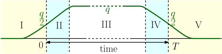
Figure 2: A schematic of the most probable trajectory of the conditioned Ornestein-Uhlenbeck process defined in Section 3.3. The most probable position changes with time, only reaching a time independent value $q=\frac{\epsilon\lambda}{\gamma^{2}}$ at the intermediate quasi-stationary region III. The evolution is symmetric under time reversal, with most probable position $\frac{q}{2}$ at $t=0$ and $t=T$.

• 1. In this example, both $X_{t}$ and $Q_{T}$ are Gaussian variables. The direct calculation of the covariance could be an alternative way of re-deriving the result (39).

  2. Here, the conditioned measure $P_{t}^{(\lambda)}(x)$ is symmetric under $t\rightarrow T-t$, thus symmetric under time reversal. This is because on a one-dimensional line the force $F(x)$ can be written as the gradient of a potential and the Langevin dynamics satisfies detailed balance. This would not necessarily be the case on a ring or in higher dimensions.

4 Large deviations in the conditioned Langevin dynamics.

We shall now discuss the Langevin dynamics on the line when the noise strength $\epsilon$ is small. This weak noise limit has been of interest in the past particularly in the Freidlin-Wentzel theory of stochastic differential equations Freidlin2012 . One may also view the fluctuating hydrodynamics description of interacting many-body systems as a generalization of the Langevin equation where the weak noise limit comes from the large system size Sadhu2016 ; Derrida2007 ; Bertini2014 ; Bertini2002 . A generalization of our discussion here to a many-body system will be presented in a future publication Sadhu2018 .

In this weak noise limit, one can describe rare fluctuations in terms of a large deviations function Freidlin2012 ; Graham1985 ; Graham1973 . For example, the steady state probability of a Langevin equation describing a particle in a potential $U(x)$ has a large deviations form

$$P(x)\sim e^{-\frac{2}{\epsilon}U(x)}\qquad\textrm{for small $\epsilon$.}$$

In this Section, we shall show that a similar large deviations description holds for the conditioned measure in the Langevin equation.

4.1 WKB solution of the eigenfunctions

For small $\epsilon$, one can try the WKB method Landau to determine the largest eigenvalue and associated eigenvectors of the tilted operator $\mathcal{L}_{\lambda}$ in (32). This means that we look for a solution of the type

$$r_{\frac{\kappa}{\epsilon}}(x)\sim e^{-\frac{1}{\epsilon}\psi_{\textrm{right}}^{(\kappa)}(x)},\qquad\ell_{\frac{\kappa}{\epsilon}}(x)\sim e^{-\frac{1}{\epsilon}\psi_{\textrm{left}}^{(\kappa)}(x)}$$ (40a)

by setting

$$\lambda=\frac{\kappa}{\epsilon}\qquad\textrm{and}\qquad\mu\left(\frac{\kappa}{\epsilon}\right)\simeq\frac{1}{\epsilon}\chi(\kappa)$$ (40b)

in the eigenvalue equations (34). We find that, for small $\epsilon$, this is indeed a consistent solution to the leading order when the large deviations functions satisfy

$$F(x)^{2}-\left(\frac{d}{dx}\psi_{\textrm{left}}^{(\kappa)}(x)-\kappa h(x)-F(x)\right)^{2}= 2\kappa f(x)-2\chi(\kappa)$$ (41a)

$$F(x)^{2}-\left(\frac{d}{dx}\psi_{\textrm{right}}^{(\kappa)}(x)+\kappa h(x)+F(x)\right)^{2}= 2\kappa f(x)-2\chi(\kappa)$$ (41b)

When we use such a solution in (33) we get

$$G_{T}^{(\frac{\kappa}{\epsilon})}(x|y)\sim e^{\frac{T}{\epsilon}\chi(\kappa)-\frac{1}{\epsilon}\psi_{\textrm{right}}^{(\kappa)}(x)-\frac{1}{\epsilon}\psi_{\textrm{left}}^{(\kappa)}(y)}$$ (42)

for small $\epsilon$. This also gives a large deviations form for the conditioned measure. In particular, the conditioned measure (13) and (17), for small $\epsilon$, gives

$$\mathcal{P}_{T}^{(\frac{\kappa}{\epsilon})}(x)\sim e^{-\frac{1}{\epsilon}\psi_{T}^{(\kappa)}(x)}\qquad\textrm{and}\qquad\mathcal{P}_{0}^{(\frac{\kappa}{\epsilon})}(x)\sim e^{-\frac{1}{\epsilon}\psi_{0}^{(\kappa)}(x)}$$ (43)

where $\psi_{T}^{(\kappa)}(x)\simeq\psi_{\textrm{right}}^{(\kappa)}(x)$ and $\psi_{0}^{(\kappa)}(x)\simeq\psi_{\textrm{left}}^{(\kappa)}(x)+\mathcal{F}(x)$ up to an additive constant (we denote by $\mathcal{F}(x)$ the large deviations function associated to the steady state probability of the original Langevin equation (27)).

• 1. The solution (42) implies that the joint probability (10) also has a large deviations form given by

     $$P_{T}(x,Q_{T}=qT|y)\sim e^{-\frac{T}{\epsilon}\Phi(q)-\frac{1}{\epsilon}\psi_{\textrm{right}}(x,q)-\frac{1}{\epsilon}\psi_{\textrm{left}}(y,q)}$$

     for small $\epsilon$, and the large deviations functions are related to their counterpart $\chi(\kappa)$, $\psi_{\textrm{right}}^{(\kappa)}(x)$, and $\psi_{\textrm{left}}^{(\kappa)}(x)$ by the ensemble equivalence

     $$\Phi(q)=\kappa\;q-\chi(\kappa)\qquad\textrm{with}\qquad\kappa=\Phi^{\prime}(q)$$ (44)

     for large $T$.

  2. Later, in Section 6.3, we will see that (41a-41b) are the Hamilton-Jacobi equations in a variational formulation of the problem.

4.2 Conditioned large deviations

The WKB solution (40a) gives that the conditioned measure at any time $t$, in the two ensembles, has a large deviations form

$$P_{t}^{(\frac{\kappa}{\epsilon})}(x)\sim e^{-\frac{1}{\epsilon}\psi_{t}^{(\kappa)}(x)}\qquad\textrm{and}\qquad\mathcal{P}_{t}(x|Q=qT)\sim e^{-\frac{1}{\epsilon}\psi_{t}(x,q)}$$ (45)

with the two conditioned large deviations functions related by the equivalence of ensembles (44). This is already seen in (43). For other times, this comes from using the WKB solution (40a-40b) in the expressions (36a-36e) for small $\epsilon$.

Among these, the simplest case is the quasi-stationary regime, i.e. $1\ll t$ and $T-t\gg 1$, where $P_{t}^{(\lambda)}(x)=r_{\lambda}(x)\ell_{\lambda}(x)$ given in (36c). Using (40a) we get

$$\psi_{t}^{(\kappa)}(x)\equiv\psi_{\textrm{mid}}^{(\kappa)}(x)=\psi_{\textrm{right}}^{(\kappa)}(x)+\psi_{\textrm{left}}^{(\kappa)}(x)$$ (46)

In other regions one could similarly derive expressions for $\psi_{t}^{(\kappa)}(x)$.

5 Gradient force

For the rest of this paper, we shall consider the Langevin equation (27) on the line where the force is the gradient of a confining potential $U(x)$, i.e. $F(x)=-\partial_{x}U(x)$. For simplicity we shall only consider $Q_{T}=\int_{0}^{T}dt\,f(X_{t})$ (i.e. $h(x)=0$ in (29)).

As a consequence, the two solutions of the Hamilton-Jacobi equations (41a-41b) are related,

$$\psi_{\textrm{left}}^{(\kappa)}(x)=\psi_{\textrm{right}}^{(\kappa)}(x)-2U(x)+\textrm{constant}$$ (47)

(This would not be true, in general, when $F(x)$ is not a gradient of a potential. For example, on a ring with a circular driving force.)

Moreover, using (47), the effective force (37b) in the quasi-stationary regime, for small $\epsilon$, can be written as

$$F_{t}^{(\frac{\kappa}{\epsilon})}(x)\simeq F(x)-\frac{d}{dx}\psi_{\textrm{left}}^{(\kappa)}(x)=-\frac{1}{2}\partial_{x}\psi_{\textrm{mid}}^{(\kappa)}(x)$$ (48)

(This is only the leading order term for small $\epsilon$.) This shows that the conditioned process can be viewed as a Langevin dynamics in the potential landscape of the conditioned large deviations function.

An explicit solution

The Hamilton-Jacobi equations (41a-41b) are simple to solve. For example, lets take (41b) which is quadratic and has two solutions $\psi_{\pm}^{(\kappa)}(x)$ which follows

$$\partial_{x}\psi_{\pm}^{(\kappa)}(x)=-F(x)\pm\sqrt{F(x)^{2}-2\kappa f(x)+2\chi(\kappa)}$$

When $F(x)^{2}-2\kappa f(x)$ has a single global minimum at a value $x=u$ and it grows at $x\rightarrow\pm\infty$ (and $F(x)$ is a gradient of a confining potential), the only possible choice is that

$$\partial_{x}\psi_{\textrm{right}}^{(\kappa)}(x)=\begin{cases}\partial_{x}\psi_{+}^{(\kappa)}(x),&\mbox{for }x\geq u,\\ \partial_{x}\psi_{-}^{(\kappa)}(x),&\mbox{for }x\leq u.\end{cases}$$

At the meeting point, the eigenfunction $r_{\frac{\kappa}{\epsilon}}(x)$ and its derivative are continuous which leads to continuity of $\partial_{x}\psi_{\textrm{right}}^{(\kappa)}(x)$. The latter condition gives

$$\chi(\kappa)=\kappa f(u)-\frac{1}{2}F(u)^{2}\qquad\textrm{with}\qquad\kappa=\frac{F(u)F^{\prime}(u)}{f^{\prime}(u)}$$ (49)

• The reason for imposing the condition that $F(x)^{2}-2\kappa f(x)$ has a single global minimum is that otherwise, one can not straightforwardly extend the asymptotic solutions $\psi_{\pm}^{(\kappa)}(x)$ to all values of $x$, similar to the WKB analysis of double well potential in Quantum Mechanics Landau . This is because between the minima the eigenfunction is a superposition of the $\psi_{+}^{(\kappa)}(x)$ and $\psi_{-}^{(\kappa)}(x)$ solutions and one has to carefully match the solutions at each minimum.

The second Hamilton-Jacobi equation (41a) is similarly solved. Integrating these solutions we write

$$\psi_{\textrm{right}}^{(\kappa)}(x)= \int_{x^{\star}}^{x}dz\;\left\{-F(z)+\textrm{sgn}(x-u)\sqrt{F(z)^{2}-F(u)^{2}-2\kappa[f(z)-f(u)]}\right\}$$ (50a)

$$\psi_{\textrm{left}}^{(\kappa)}(x)= K+\int_{x^{\star}}^{x}dz\;\left\{F(z)+\textrm{sgn}(x-u)\sqrt{F(z)^{2}-F(u)^{2}-2\kappa[f(z)-f(u)]}\right\}$$ (50b)

where $K$ and $x^{\star}$ are a priori arbitrary constants. To satisfy the normalization $\int dx\,r_{\lambda}(x)\ell_{\lambda}(x)=1$, one can choose $K=0$ for $x^{\star}=u$ (using $F(x)^{2}-2\kappa f(x)$ has minimum at $x=u$).

Using (50a-50b) in (43) one can see that $\psi_{T}^{(\kappa)}(x)$ and $\psi_{0}^{(\kappa)}(x)$ both have minimum at $x_{0}$ given by $f(x_{0})=f(u)-\frac{1}{2\kappa}F(u)^{2}$. This makes $x_{0}$ the most likely position at time $t=0$ and $t=T$ which is different from the quasi-stationary position $u$.

As a consequence of (50a-50b) we get the conditioned large deviations function (46) in the quasi-stationary regime

$$\psi_{\textrm{mid}}^{(\kappa)}(x)=2\,\textrm{sgn}(x-u)\int_{u}^{x}dz\;\sqrt{F(z)^{2}-F(u)^{2}-2\kappa[f(z)-f(u)]}$$ (51)

This shows that $x=u$ is the most likely position in the quasi-stationary regime.

• 1. In this example, one could systematically calculate sub-leading corrections in the eigenvalue and eigenvector. Writing

     $$r_{\frac{\kappa}{\epsilon}}(x)=e^{-\frac{1}{\epsilon}\psi_{\textrm{right}}^{(\kappa)}(x)-\widetilde{\psi}_{\textrm{right}}^{(\kappa)}(x)+\cdots},\qquad\mu\left(\frac{\kappa}{\epsilon}\right)=\frac{1}{\epsilon}\chi(\kappa)+\widetilde{\chi}(\kappa)+\cdots$$

     in (34) (we are using $h(x)=0$) and expanding in powers of $\epsilon$ one would get in the sub-leading order

     $$-F^{\prime}(x)+\left[F(x)+\partial_{x}\psi_{\textrm{right}}^{(\kappa)}(x)\right]\partial_{x}\widetilde{\psi}_{\textrm{right}}^{(\kappa)}(x)-\frac{1}{2}\partial_{x}^{2}\psi_{\textrm{right}}^{(\kappa)}(x)=\widetilde{\chi}(\kappa)$$ (52)

     Using (50a) we see that the term $F(x)+\partial_{x}\psi_{\textrm{right}}^{(\kappa)}(x)$ in (52) vanishes at $x=u$. Moreover, from (50a) we get

     $$\lim_{x\rightarrow u}\partial_{x}^{2}\psi_{\textrm{right}}^{(\kappa)}(x)=-F^{\prime}(u)+\sqrt{F^{\prime}(u)^{2}+F(u)F^{\prime\prime}(u)-\kappa f^{\prime\prime}(u)}$$

     This and the fact that $\partial_{x}\psi_{\textrm{right}}^{(\kappa)}(x)=-F(x)$ for $x=u$ gives for the sub-leading order correction to the eigenvalue

     $$\widetilde{\chi}(\kappa)=-\frac{1}{2}\left[F^{\prime}(u)+\sqrt{F^{\prime}(u)^{2}+F(u)F^{\prime\prime}(u)-\kappa f^{\prime\prime}(u)}\right]$$ (53)

     An explicit expression for $\widetilde{\psi}_{\textrm{right}}^{(\kappa)}(x)$ could also be deduced from (50a) and (52).

  2. One can also check that the results for the Ornstein-Uhlenbeck process in Section 3.3 can be recovered by choosing $f(x)=x$ and $F(x)=-\gamma x$.

6 A variational formulation

The path integral formulation of the Langevin equation offers an alternative approach for the conditioned dynamics. In this, the conditioned large deviations function is obtained as a solution of a variational problem. As in Section 5, we consider a gradient force and $Q_{T}=\int_{0}^{T}dt\,f(X_{t})$, although one could extend the analysis for other cases.

We introduce the formulation for the generating function $G_{T}^{(\lambda)}(x|y)$ for the Langevin dynamics. Using a path integral solution of (31) (see Appendix D for details) one can write, for small $\epsilon$,

$$G_{T}^{(\frac{\kappa}{\epsilon})}(x|y)\sim\int_{z(0)=y}^{z(T)=x}\mathcal{D}[z]e^{\frac{1}{\epsilon}S_{T}^{(\kappa)}[z(t)]}$$ (54)

where the Action

$$S_{T}^{(\kappa)}[z]=\int_{0}^{T}dt\left\{\kappa\,f(z)-\frac{\dot{z}^{2}}{2}+\dot{z}\,F(z)-\frac{F(z)^{2}}{2}\right\}$$ (55)

One may view (54) as a sum over all paths (connecting $y$ to $x$ during time $T$) weighted by $\exp(\frac{1}{\epsilon}S_{T}^{(\kappa)}[z])$.

In the small $\epsilon$ limit, if we assume that (54) is dominated by a single path, we get (42) with

$$T\chi(\kappa)-\psi_{\textrm{right}}^{(\kappa)}(x)-\psi_{\textrm{left}}^{(\kappa)}(y)=\max_{z(t)}S_{T}^{(\kappa)}[z(t)]$$ (56)

where the maximum is over all possible trajectories $z(t)$ with $z(0)=y$ and $z(T)=x$.

6.1 An explicit solution

Let us first show how this variational approach allows one to recover the results of Section 5. As before, we limit our discussions to the case where $F^{2}(z)-2\kappa\,f(z)$ has a single global minimum at $x=u$. It will be clear shortly, that in the variational formulation, this condition ensures a single time independent optimal path.

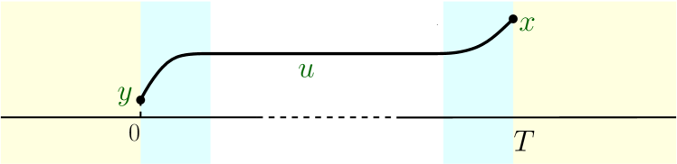
Figure 3: A schematic of the optimal path for the variational problem in Section 6.1.

Using variational calculus we get from (54-55) that the optimal path follows

$$\ddot{z}=\frac{d}{dz}\left[\frac{F(z)^{2}}{2}-\kappa f(z)\right]$$

Multiplying the above equation with $2\dot{z}$ and integrating we get

$$\dot{z}^{2}=F(z)^{2}-2\kappa f(z)+K$$

where $K$ is an integration constant. We see the similarity with the trajectory of a mechanical particle of constant energy $\frac{1}{2}K$ in a potential $\kappa f(z)-\frac{F(z)^{2}}{2}$ which has a single global maximum at $x=u$. The trajectory has to cover a finite distance from the point $y$ to the point $x$ in a very large time $T$. The only possible way this could happen if the trajectory passes arbitrarily close to $u$ which is a repulsive fixed point of the mechanical dynamics. This requires an energy almost equal to the maximum of the mechanical potential, with the difference vanishing as $T$ grows. This gives $K=2\kappa f(u)-F(u)^{2}$ and the optimal path

$$\dot{z}^{2}=F(z)^{2}-2\kappa f(z)+2\kappa f(u)-F(u)^{2}$$ (57)

Such a trajectory spends most of its time in the position $u$, and deviates from it only near the boundary to comply with the condition $z(0)=y$ and $z(T)=x$, as sketched in Figure 3. Then, we can write the optimal path (57), for large $T$, as

$$\dot{z}(t)=\begin{cases}\textrm{sgn}(u-y)\sqrt{F(z)^{2}-2\kappa f(z)+2\kappa f(u)-F(u)^{2}},&\textrm{for $0\leq t\ll T$,}\\ 0,&\textrm{for $1\ll t$ and $T-t\gg 1$,}\\ \textrm{sgn}(x-u)\sqrt{F(z)^{2}-2\kappa f(z)+2\kappa f(u)-F(u)^{2}},&\textrm{for $0\leq T-t\ll T$.}\end{cases}$$

To use this in the variational formula (56) we substitute $F(z)^{2}$ from (57) in the expression (55) and get

$$\max_{z(t)}S_{T}^{(\kappa)}[z(t)]=T\left[\kappa\,f(u)-\frac{1}{2}F(u)^{2}\right]+\int_{0}^{t_{0}}dt\,\dot{z}\,\left[F(z)-\dot{z}\right]+\int_{t_{0}}^{T}dt\,\dot{z}\left[F(z)-\dot{z}\right]$$

where $t_{0}\in[0,T]$. We see that, the integration variable can be changed to $z$, and when $1\ll t_{0}$ and $T-t_{0}\gg 1$, we can use $z(t_{0})=u$, in addition to the boundary condition $z(0)=y$ and $z(T)=x$. Using the explicit solution of $\dot{z}(t)$, given above, we get

$$\max_{z(t)}S_{T}^{(\kappa)} [z(t)]=T\left[\kappa\,f(u)-\frac{1}{2}F(u)^{2}\right]$$

$$- \int_{u}^{y}dz\,\left[F(z)+\textrm{sgn}(y-u)\sqrt{F(z)^{2}-2\kappa f(z)+2\kappa f(u)-F(u)^{2}}\right]$$

$$- \int_{u}^{x}dz\,\left[-F(z)+\textrm{sgn}(x-u)\sqrt{F(z)^{2}-2\kappa f(z)+2\kappa f(u)-F(u)^{2}}\right]$$

When we use this result in the variational formula (56) for large $T$, we get $\chi(\kappa)=\left[\kappa\,f(u)-\frac{1}{2}F(u)^{2}\right]$, in agreement with our earlier result in (49). Moreover, we see that the second and third term gives $\psi_{\textrm{left}}^{(\kappa)}(y)$ and $\psi_{\textrm{right}}^{(\kappa)}(x)$ in (50a-50b).

6.2 Conditioned large deviations function

One could write a similar variational formula for the conditioned large deviations function $\psi_{t}^{(\kappa)}(x)$ at an arbitrary time $t$. For large $T$,

$$\psi_{t}^{(\kappa)}(x)\simeq\max_{z}A_{T}^{(\kappa)}[z(\tau)]-\max_{z(t)=x}A_{T}^{(\kappa)}[z(\tau)]$$ (58a)

where the action

$$A_{T}^{(\kappa)}[z(\tau)]=\int_{-\infty}^{\infty}d\tau\left\{a(\tau)\,f(z)-\frac{\dot{z}^{2}}{2}+\dot{z}\,F(z)-\frac{F(z)^{2}}{2}\right\}$$ (58b)

with $a(\tau)=\kappa$ for $\tau\in[0,T]$ and $a(\tau)=0$ elsewhere. The first maximization in (58a) is over all paths, whereas the second maximization is over paths which are conditioned to be at $z(\tau)=x$ for $\tau=t$.

One may understand the formula (58a) as an optimal contribution from an ensemble of paths with probability weight $e^{\frac{1}{\epsilon}A_{T}^{(\kappa)}[z]}$ conditioned to pass through $x$ at time $t$; the first term in (58a) is due to normalization.

Here, we show how one can use this variational approach to derive the conditioned large deviations function at an arbitrary time. For this we impose as in Section 6.1 that $F(x)^{2}-2\kappa\,f(x)$ has a single global minimum such that the most likely position in the quasi-stationary regime is time independent, $z(\tau)=u$.

Quasi-stationary regime.

Among all the five regions in Figure 1, the simplest is to analyze the quasi-stationary regime where $1\ll t$ and $T-t\gg 1$. Here, for the optimization in (58a), one essentially need to consider paths which asymptotically reach $u$, both at small $t$, as well as when $t$ is close to $T$. A schematic such path is given in Figure 4.

Figure 4: A schematic of a path leading to a fluctuation $x$ at time $t$, and subsequent relaxation to the quasi-stationary value $u$ in region III.

The analysis is quite similar to that in Section 6.1. We get that the optimal path follows

$$\frac{dz(\tau)}{d\tau}=\begin{cases}\textrm{sgn}(x-u)\sqrt{F(z)^{2}-2\kappa f(z)+2\kappa f(u)-F(u)^{2}},&\textrm{for $\tau<t$}\\ \textrm{sgn}(u-x)\sqrt{F(z)^{2}-2\kappa f(z)+2\kappa f(u)-F(u)^{2}},&\textrm{for $\tau>t$,}\end{cases}$$ (59)

and using this in (58a) we get

$$\psi_{t}^{(\kappa)}(x)=\int_{0}^{t}d\tau\,\dot{z}\left[\dot{z}-F(z)\right]+\int_{t}^{T}d\tau\,\dot{z}\left[\dot{z}-F(z)\right]$$

Changing the integration variable to $z$ and using the solution (59) with the asymptotics sketched in Figure 4, we get

$$\psi_{t}^{(\kappa)}(x)= \int_{u}^{x}dz\left[-F(z)+\textrm{sgn}(x-u)\sqrt{F(z)^{2}-2\kappa f(z)+2\kappa f(u)-F(u)^{2}}\right]$$

$$+\int_{u}^{x}dz\left[F(z)+\textrm{sgn}(x-u)\sqrt{F(z)^{2}-2\kappa f(z)+2\kappa f(u)-F(u)^{2}}\right]$$

Comparing with the expression in (50a-50b) we see that $\psi_{t}^{(\kappa)}(x)=\psi_{\textrm{right}}^{(\kappa)}(x)+\psi_{\textrm{left}}^{(\kappa)}(x)$, in agreement with our earlier result (46) and (51).

• From (59) one could see that the optimal path leading to a fluctuation in the quasi-stationary regime and subsequent relaxation follows a deterministic evolution in a potential landscape of conditioned large deviations function.

  $$\frac{dz(\tau)}{d\tau}= F(z)+\frac{d}{dz}\psi_{\textrm{right}}^{(\kappa)}(z)=-\frac{d}{dz}\left[U(z)-\psi_{\textrm{right}}^{(\kappa)}(z)\right]\quad\mbox{for }\tau<t,$$ (60a)

  $$\frac{dz(\tau)}{d\tau}= F(z)-\frac{d}{dz}\psi_{\textrm{left}}^{(\kappa)}(z)=-\frac{d}{dz}\left[U(z)+\psi_{\textrm{left}}^{(\kappa)}(z)\right]\qquad\mbox{for }\tau>t.$$ (60b)

Region II $(0\leq t\ll T)$.

The calculation of $\psi_{t}^{(\kappa)}(x)$ in other regions of time is quite similar. For example, in region II, in the variational formula (58a), one essentially need to consider paths which started at the minimum of $U(x)$ (with $F(x)=-U^{\prime}(x)$) when $\tau\rightarrow-\infty$, pass through $z=x$ at $\tau=t\geq 0$, and asymptotically reach the quasi-stationary value $u$ for large time $\tau\gg 1$, as illustrated in Figure 5.

Following an analysis similar to that in Section 6.1 it is straightforward to show that the optimal path in this case

$$\dot{z}(\tau)=\begin{cases}-F(z),&\textrm{for $\tau\leq 0$}\\ \textrm{sgn}(x-y)\sqrt{F(z)^{2}-2\kappa f(z)+K_{1}},&\textrm{for $0\leq\tau\leq t$}\\ \textrm{sgn}(u-x)\sqrt{F(z)^{2}-2\kappa f(z)+K_{2}},&\textrm{for $\tau\geq t$,}\end{cases}$$ (61)

where $K_{1}$ and $K_{2}$ are integration constants, and the optimal path passes through $z(0)=y$ (say) when $\tau=0$. The solution for $\tau\leq 0$ is easy to see from the condition that at $\tau\rightarrow-\infty$ the system started at the minimum of the potential $U(z)$ with $F(z)=-U^{\prime}(z)$. Similar asymptotics that for large time the system relaxes to the quasi-stationary position $z=u$ gives the constant $K_{2}=2\kappa f(u)-F(u)^{2}$. In addition, we have the condition

$$t=\int_{0}^{t}d\tau=\int_{y}^{x}\frac{dz}{\dot{z}}=\int_{y}^{x}\frac{dz}{\textrm{sgn}(x-y)\sqrt{F(z)^{2}-2\kappa f(z)+K_{1}}}$$ (62)

where we used the solution (61) and this fixes the constant $K_{1}$.

When we use the solution (61) to write $F(z)^{2}$ in the expression (58b), we get

$$\max_{z(t)=x}A_{T}^{(\kappa)}[z(\tau)]=(T-t)\left[\kappa f(u)-\frac{F(u)^{2}}{2}\right]+t\,\frac{K_{1}}{2}-\int_{-\infty}^{T}d\tau\,\dot{z}\big{[}\dot{z}-F(z)\big{]}$$

Using this in (58a) and the result that $\max_{z(t)}A_{T}^{(\kappa)}[z(\tau)]=T\left[\kappa f(u)-\frac{F(u)^{2}}{2}\right]$, we get

$$\psi_{t}^{(\kappa)}(x)=t\left[\kappa f(u)-\frac{F(u)^{2}}{2}\right]-t\,\frac{K_{1}}{2}+\int_{-\infty}^{T}d\tau\,\dot{z}\big{[}\dot{z}-F(z)\big{]}$$

In this expression, the integration variable can be changed from $\tau$ to $z$, and then using the explicit solution (61), we get

$$\psi_{t}^{(\kappa)}(x)=t\left[\kappa f(u)-\frac{F(u)^{2}}{2}\right]+\psi_{\textrm{left}}^{(\kappa)}(x)+\widehat{B}_{t}^{(\kappa)}(x,y)+\mathcal{F}(y)$$ (63a)

where $$\psi_{\textrm{left}}^{(\kappa)}(x) \mathcal{F}(y)=-2\int_{0}^{y}dz\,F(z)$$ is given in (50b), and

$$\widehat{B}_{t}^{(\kappa)}(x,y)=-t\,\frac{K_{1}}{2}+\int_{y}^{x}dz\left[-F(z)+\textrm{sgn}(x-y)\sqrt{F(z)^{2}-2\kappa f(z)+K_{1}}\right]$$ (63b)

We note that the condition (62) is equivalent to $\partial_{K_{1}}\widehat{B}_{t}^{(\kappa)}(x,y)=0$, which relates $K_{1}$ to $y$. In addition, the solution (63a) must be optimal over a variation in $y$. These two conditions together leads to $\partial_{y}\widehat{B}_{t}^{(\kappa)}(x,y)=2F(y)$, which with the formula (63b) gives $K_{1}=2\kappa\,f(y)$. We note that this is equivalent of continuity of $\dot{z}(\tau)$ at $\tau=0$ in the solution (61). This result for $K_{1}$, along with (62) and (63a-63b) gives a parametric solution of $\psi_{t}^{(\kappa)}(x)$ in region II.

We have checked that the same result could be derived using the eigenfunction of the tilted Fokker-Planck operator discussed earlier in Section 4.

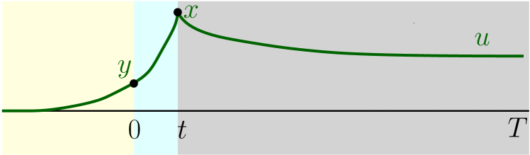
Figure 5: A schematic of a path leading to a fluctuation $x$ at $t$ in region II, and subsequent relaxation to the quasistationary position $u$.

6.3 The Hamilton-Jacobi equations from the variational approach

In Section 4.1 we have shown how one can write the conditioned large deviations function in terms of a solution of the Hamilton-Jacobi equations (41a, 41b) derived from the tilted Fokker-Planck operator. In this section, we describe how the same equations can be obtained using the variational formulation in Section 6. The advantage is that in more general problems, e.g. the fluctuating hydrodynamics of interacting many-body systems, this variational approach is simpler than using the tilted Fokker-Planck operator (see our future publication Sadhu2018 ).

We start with a derivation of (41a). Using the definition (6) one can write for the Langevin equation

$$G_{T}^{(\lambda)}(x|y)=\int dz\,G_{T-t}^{(\lambda)}(x|z)G_{t}^{(\lambda)}(z|y)$$ (64)

A schematic illustrating this time convolution is shown in Figure 6.

Figure 6: A schematic of the sample of paths contributing in the time convolution in (64).

Using the large deviations form (42) and the path integral representation (54), for small $\epsilon$, it is straightforward to write

$$t\,\chi(\kappa)-\psi_{\textrm{left}}^{(\kappa)}(y)\simeq\max_{z}\left\{S_{t}^{(\kappa)}(z,y)-\psi_{\textrm{left}}^{(\kappa)}(z)\right\}$$ (65)

where, from the Action (55), we get for small $t$,

$$S_{t}^{(\kappa)}(z,y)=t\,\kappa f(y)-\frac{1}{2}\left[\frac{(z-y)}{t}-F(y)\right]^{2}+\cdots$$

Expanding (65) around $y$ we get

$$\chi(\kappa)\simeq\kappa\,f(y)-\frac{F(y)^{2}}{2}+\frac{1}{t}\max_{z}\left\{(z-y)[F(y)-\partial_{y}\psi_{\textrm{left}}^{(\kappa)}(y)]-\frac{(z-y)^{2}}{2\,t}\right\}$$

Higher order terms in the expansion are negligible in the small $t$ limit.

In this expression, the maximum is for

$$\frac{(z-y)}{t}=F(y)-\partial_{y}\psi_{\textrm{left}}^{(\kappa)}(y)$$

Substituting this in the above expression for $\chi(\kappa)$ and taking $t\rightarrow 0$ limit we recover the Hamilton-Jacobi equation (41a) for $h(x)=0$. One can similarly derive the Hamilton-Jacobi equation (41b) for $\psi_{\textrm{right}}^{(\kappa)}(x)$. The analysis could be extended for $h(x)\neq 0$, as well.

7 The effect of conditioning on the noise.

In (37a-37d) we have seen that the Langevin dynamics conditioned on $Q_{T}=\int_{0}^{T}dt\,f(x)$ can be described by another Langevin dynamics with an effective force $F_{t}^{(\lambda)}(x)$ and white noise $\widetilde{\eta}_{t}$. In the weak noise limit, the effective force in the quasi-stationary regime ($t\gg 1$ and $T-t\gg 1$) is given by (48) with (51). So the conditioned dynamics, for small $\epsilon$, is

$$\dot{X}_{t}=-\textrm{sgn}(X_{t}-u)\sqrt{F(X_{t})^{2}-F(u)^{2}-2\kappa[f(X_{t})-f(u)]}+\widetilde{\eta}_{t}$$

where $\widetilde{\eta}_{t}$ is a Gaussian white noise as in the original (unconditioned) Langevin equation (27).

In this quasi-stationary regime, the most probable position $X_{t}=u$ is time independent (under the condition that $F(x)^{2}-2\kappa f(x)$ has a single global minimum). Writing small fluctuations $r_{t}=X_{t}-u$ we get from the above equation

$$\dot{r}_{t}=-\Gamma_{u}\,r_{t}+\widetilde{\eta}_{t},\qquad\textrm{with}\qquad\Gamma_{u}=\sqrt{F^{\prime}(u)^{2}+F(u)F^{\prime\prime}(u)-\kappa f^{\prime\prime}(u)}$$

The solution

$$r_{t}=\int_{-\infty}^{t}ds\,e^{-\Gamma_{u}\,(t-s)}\,\widetilde{\eta}_{s}$$

leads to the following correlation

$$\left\langle X_{t}X_{t^{\prime}}\right\rangle_{c}=\left\langle r_{t}r_{t^{\prime}}\right\rangle=\frac{\epsilon}{2\Gamma_{u}}e^{-\Gamma_{u}|t-t^{\prime}|}$$ (66)

If we come back to the original Langevin equation (27),

$$\dot{X}_{t}=F(X_{t})+\eta_{t}$$ (67)

then the original noise, when the fluctuation $r_{t}=X_{t}-u$ is small, is given by

$$\eta_{t}\simeq-F(u)+\dot{r}_{t}-F^{\prime}(u)\,r_{t}$$ (68)

Then, using the correlation (66) one gets

$$\left\langle X_{t}\,\eta_{t^{\prime}}\right\rangle_{c}=\left\langle r_{t}\,\eta_{t^{\prime}}\right\rangle=\begin{cases}g_{R}(t^{\prime}-t),&\textrm{ for $t^{\prime}>t$}\\ g_{F}(t-t^{\prime}),&\textrm{ for $t^{\prime}<t$}\end{cases}$$ (69a)

where

$$g_{F}(t)={-F^{\prime}(u)+\Gamma_{u}\over 2\Gamma_{u}}e^{-\Gamma_{u}t}\qquad\textrm{and}\qquad g_{R}(t)={-F^{\prime}(u)-\Gamma_{u}\over 2\Gamma_{u}}e^{-\Gamma_{u}t}$$ (69b)

In this description, we see that the fluctuation $r_{t}$ is correlated not only to the noise in the past, but also to the noise in the future. Of course, when one removes the conditioning, i.e. for $\kappa=0$, and as a result $u=0$, one has $\Gamma_{0}=F^{\prime}(0)$ and $g_{R}=0$, as one would expect in a Markovian process. One can also show, using (66) and (68), that

$$\left\langle\eta_{t}\right\rangle=-F(u)\qquad\textrm{and}\qquad\langle\eta_{t}\eta_{t^{\prime}}\rangle=\epsilon\,\frac{F^{\prime}(u)^{2}-\Gamma_{u}^{2}}{2\Gamma_{u}}\,e^{-\Gamma_{u}|t-t^{\prime}|}$$ (70)

so that the original noise $\eta_{t}$ becomes colored due to the conditioning.

8 Summary

In this work we have seen how a stochastic system adapts its dynamics when it is conditioned on a certain value of an empirical observable $Q_{T}$ of the form (4). The constrained dynamics remains Markovian (see (19, 25)) if the original process is itself Markovian. In the case of the Langevin dynamics, the conditioning modifies the force (see (37a-37d)). The large $T$ limit leads to an equivalence of ensembles between the microcanonical ensemble (where conditioning is on a fixed value of $Q_{T}$, defined in (4) and (29)) and the canonical ensemble (where the dynamics is weighted by $e^{\lambda\,Q_{T}}$). This is similar to the equivalence of thermodynamic ensembles in equilibrium when volume is large.

In the weak noise limit of the Langevin dynamics, one can introduce conditioned Large deviations functions which characterize fluctuations in the conditioned dynamics. Using a WKB solution we showed in Section 4.1 that these conditioned large deviations functions can be expressed in terms of the solution of the Hamilton-Jacobi equations (41a-41b). The same result can also be derived (see Section 6) using a variational formulation, where the large deviations functions are related to the minimum of the Action that characterizes the path-space probability. Within this variational approach, one can calculate the optimal trajectory which describes how atypical fluctuations are generated and how they relax (59, 61). A similar approach to our variational formulation was also used recently Nicolas2018 in the quasi-stationary regime of a Langevin dynamics in a periodic potential.

One of the rather surprising aspects in the Langevin dynamics is that the noise becomes correlated over time due to the conditioning (see (70)). Moreover, fluctuations of the position at a time become correlated to the noise in the future.

The examples discussed in this paper are simple as they deal with a single degree of freedom. They are part of a theory which is rather general. In a forthcoming publication Sadhu2018 we shall apply the same ideas for a system with many degrees of freedom Bertini2014 ; Derrida2007 ; Hurtado2014 , e.g. the symmetric exclusion process. The variational approach discussed here for the Langevin dynamics can be generalized for the large systems where the weak noise limit comes from the large volume. Several of the ideas used in this paper will be extended there.

We have seen in (16c) and (36c) that in the quasi-stationary regime the conditioned measure is a product of the left and right eigenvectors corresponding to the largest eigenvalue of the tilted matrix. Even in the non-stationary regime (see (23a)) the conditioned measure is a product of a left vector and a right vector which evolve according to linear equations. This is very reminiscent of Quantum Mechanics. What could be learnt from this analogy is an interesting open issue.

Appendix A Ensemble equivalence

In this appendix we show that, for large $T$, the equivalence of ensembles holds for an arbitrary time $t$.

As the reasoning is very similar in the five regions of figure 1, we will limit our discussion to the case of region II, i.e. for $0\leq t\ll T$. Let $P_{t}(C_{T},C,Q|C_{0})$ be the joint probability of configuration $C_{T}$ at time $T$, configuration $C$ at time $t$ and of the observable $Q_{T}$ to take value $Q$ given its initial configuration $C_{0}$ at time $0$.

To establish the equivalence of ensembles in (15), we need to show that the micro-canonical probability

$$\mathcal{P}_{t}(C|Q=qT)=\frac{\sum_{C_{T}}\sum_{C_{0}}P_{t}(C_{T},C,Q=qT|C_{0})R_{0}(C_{0})}{\sum_{C^{\prime}}\left[\sum_{C_{T}}\sum_{C_{0}}P_{t}(C_{T},C^{\prime},Q=qT|C_{0})R_{0}(C_{0})\right]}$$ (71)

and the canonical probability

$$P_{t}^{(\lambda)}(C)=\frac{\sum_{C_{T}}\sum_{C_{0}}\int dQ\,e^{\lambda Q}P_{t}(C_{T},C,Q|C_{0})R_{0}(C_{0})}{\sum_{C^{\prime}}\left[\sum_{C_{T}}\sum_{C_{0}}\int dQ\,e^{\lambda Q}P_{t}(C_{T},C^{\prime},Q|C_{0})R_{0}(C_{0})\right]}$$ (72)

converge to the same distribution for large $T$ when $\lambda$ and $q$ are related by (11).

For this we write in terms of the probability (5),

$$P_{t}(C_{T},C,Q=qT|C_{0})=\int dQ_{t}\;P_{T-t}(C_{T},qT-Q_{t}|C)\;P_{t}(C,Q_{t}|C_{0})$$ (73)

and use the result (10). For large $T$, one has

$$P_{T-t}(C_{T},qT-Q_{t}|C)\simeq e^{-(T-t)\phi(q)-(tq-Q_{t})\phi^{\prime}(q)}\sqrt{\frac{\phi^{\prime\prime}(q)}{2\pi T}}R_{\phi^{\prime}(q)}(C_{T})L_{\phi^{\prime}(q)}(C)$$

Substituting in (71) and simplifying the expression for large $T$ we get the micro-canonical probability

$$P_{t}(C|Q=qT)\simeq\frac{L_{\phi^{\prime}(q)}(C)\sum_{C_{0}}G_{t}^{(\phi^{\prime}(q))}(C|C_{0})\;R_{0}(C_{0})}{\sum_{C^{\prime}}L_{\phi^{\prime}(q)}(C^{\prime})\sum_{C_{0}}G_{t}^{(\phi^{\prime}(q))}(C^{\prime}|C_{0})\;R_{0}(C_{0})}$$ (74)

where $G_{t}^{(\lambda)}(C|C_{0})$ is defined in (6). On the other hand, using (9) for large $T$ we get the canonical probability

$$P_{t}^{(\lambda)}(C)\simeq\frac{L_{\lambda}(C)\sum_{C_{0}}G_{t}^{(\lambda)}(C|C_{0})\;R_{0}(C_{0})}{\sum_{C^{\prime}}L_{\lambda}(C^{\prime})\sum_{C_{0}}G_{t}^{(\lambda)}(C^{\prime}|C_{0})\;R_{0}(C_{0})}$$ (75)

Clearly the two probabilities in the two ensembles coincide for $\lambda=\phi^{\prime}(q)$. Replacing $G_{t}^{(\lambda)}(C|C_{0})$ by $M_{\lambda}^{t}(C,C_{0})$ in (75) leads to the conditioned measure (16b).

The same reasoning can be easily adapted in the other regions of Figure 1.

Appendix B Continuous time Markov process

In this Appendix, we describe a continuous time limit of the Markov process, illustrated in Figure 7. In this, the empirical observable analogous to (4) is the $dt\rightarrow 0$ limit of

$$Q_{T}=dt\sum_{i=0}^{\frac{T}{dt}-1}f(C_{i})+\sum_{n}g(C_{n}^{+},C_{n}^{-})$$ (76)

where $t=i\,dt$, and $(C_{n}^{-},C_{n}^{+})$ are the configurations before and after the $n$th jump during the time interval $[0,T]$.

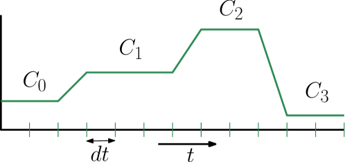
Figure 7: A schematic of a time evolution in a Markov process with discrete time steps $dt$. The continuos time limit is obtained by taking $dt\rightarrow 0$ limit.

From (7) we get

$$G_{T}^{(\lambda)}(C^{\prime}|C_{0})=\sum_{C}M_{\lambda}(C^{\prime},C)\,G_{T-dt}^{(\lambda)}(C|C_{0})$$

where

$$M_{\lambda}(C^{\prime},C)=\begin{cases}M_{0}(C^{\prime},C)e^{\lambda[dt\,f(C)+g(C^{\prime},C)]}&\textrm{for $C^{\prime}\neq C$,}\cr M_{0}(C,C)e^{\lambda\,dt\,f(C)}&\textrm{for $C^{\prime}=C$.}\end{cases}$$

Using the construction (26) for $M_{0}(C^{\prime},C)$ we take the continuous time limit $dt\rightarrow 0$ and get

$$\frac{d}{dT}G_{T}^{(\lambda)}(C^{\prime}|C_{0})=\sum_{C}\mathcal{M}_{\lambda}(C^{\prime},C)G_{T}^{(\lambda)}(C|C_{0})$$ (77)

where $\mathcal{M}_{\lambda}$ is the tilted matrix for the continuous time process,

$$\mathcal{M}_{\lambda}(C^{\prime},C)=\begin{cases}e^{\lambda g(C^{\prime},C)}\mathcal{M}_{0}(C^{\prime},C)&\textrm{for }C^{\prime}\neq C,\\ \lambda f(C)-\sum_{C^{{}^{\prime\prime}}\neq C}\mathcal{M}_{0}(C^{{}^{\prime\prime}},C)&\textrm{for }C^{\prime}=C.\end{cases}$$ (78)

This shows that the generating function is the $(C,C_{0})$th element of $e^{T\mathcal{M}_{\lambda}}$, i.e.

$$G_{T}^{(\lambda)}(C|C_{0})=e^{T\mathcal{M}_{\lambda}}(C,C_{0})$$ (79)

Although (77) resembles a Master equation, the tilted matrix $\mathcal{M}_{\lambda}$ is not a Markov matrix as $\sum_{C^{\prime}}\mathcal{M}_{\lambda}(C^{\prime},C)$ does not necessarily vanish.

For large $T$, one would get $G_{T}^{(\lambda)}(C|C_{0})\simeq e^{T\mu(\lambda)}R_{\lambda}(C)L_{\lambda}(C_{0})$ where the cumulant generating function $\mu(\lambda)$ is the largest eigenvalue of $\mathcal{M}_{\lambda}$ with $L_{\lambda}(C)$ and $R_{\lambda}(C)$ being the left and right eigenvectors, respectively. (Note the difference with the discrete time case (9) where $\mu(\lambda)$ is the logarithm of the largest eigenvalue of the tilted matrix $M_{\lambda}$ in (8).)

In a similar construction, one could get the continuous time limit of the conditioned measure (16a)-(16d) and its time evolution (18a)-(18d). The analysis is straightforward and we present only the final result.

The time evolution of conditioned measure $P_{t}^{(\lambda)}(C)$ for a continuous time Markov process is also a Markov process

$$\frac{d}{dt}P_{t}^{(\lambda)}(C^{\prime})=\sum_{C}\mathcal{W}_{t}^{(\lambda)}(C^{\prime},C)P_{t}^{(\lambda)}(C)$$ (80)

where $\mathcal{W}_{t}^{(\lambda)}(C^{\prime},C)$ is the transition rate from $C$ to $C^{\prime}$ at time $t$ in the canonical ensemble. The conditioned measure and transition rate have different expressions in the five regions indicated in Figure 1. Their expression is given below where we use a matrix product notation, e.g. $[L_{\lambda}\mathcal{M}_{\lambda}](C)\equiv\sum_{C^{\prime}}L_{\lambda}(C^{\prime})\mathcal{M}_{\lambda}(C^{\prime},C)$.

1. Region I.

   $$P_{t}^{(\lambda)}(C)= \frac{[L_{\lambda}e^{-t\mathcal{M}_{0}}](C)R_{0}(C)}{\sum_{C^{\prime}}L_{\lambda}(C^{\prime})R_{0}(C^{\prime})}$$ (81a)

   $$\mathcal{W}_{t}^{(\lambda)}(C^{\prime},C)= {[L_{\lambda}e^{-t\mathcal{M}_{0}}](C^{\prime})\over[L_{\lambda}e^{-t\mathcal{M}_{0}}](C)}\mathcal{M}_{0}(C^{\prime},C)-{\left[L_{\lambda}e^{-t\mathcal{M}_{0}}\mathcal{M}_{0}\right](C)\over[L_{\lambda}e^{-t\mathcal{M}_{0}}](C)}\;\delta_{C^{\prime},C}$$ (81b)

2. Region II.

   $$P_{t}^{(\lambda)}(C) =\frac{L_{\lambda}(C)[e^{t\mathcal{M}_{\lambda}}R_{0}](C)}{e^{t\mu(\lambda)}\sum_{C^{\prime}}L_{\lambda}(C^{\prime})R_{0}(C^{\prime})}$$ (82a)

   $$\mathcal{W}_{t}^{(\lambda)}(C^{\prime},C) ={L_{\lambda}(C^{\prime})\over L_{\lambda}(C)}\mathcal{M}_{\lambda}(C^{\prime},C)-\mu(\lambda)\delta_{C^{\prime},C}$$ (82b)

3. Region III.

   $$P_{t}^{(\lambda)}(C) =L_{\lambda}(C)R_{\lambda}(C)$$ (83a)

   $$\mathcal{W}_{t}^{(\lambda)}(C^{\prime},C) ={L_{\lambda}(C^{\prime})\over L_{\lambda}(C)}\mathcal{M}_{\lambda}(C^{\prime},C)-\mu(\lambda)\delta_{C^{\prime},C}$$ (83b)

4. Region IV.

   $$P_{t}^{(\lambda)}(C)= \frac{[L_{0}\,e^{(T-t)\mathcal{M}_{\lambda}}](C)R_{\lambda}(C)}{e^{(T-t)\mu(\lambda)}\sum_{C^{\prime}}R_{\lambda}(C^{\prime})}$$ (84a)

   $$\mathcal{W}_{t}^{(\lambda)}(C^{\prime},C)= {[L_{0}\,e^{(T-t)\mathcal{M}_{\lambda}}](C^{\prime})\over[L_{0}\,e^{(T-t)\mathcal{M}_{\lambda}}](C)}\mathcal{M}_{\lambda}(C^{\prime},C)-{\left[L_{0}\,e^{(T-t)\mathcal{M}_{\lambda}}\mathcal{M}_{\lambda}\right](C)\over\left[L_{0}\,e^{(T-t)\mathcal{M}_{\lambda}}\right](C)}\delta_{C^{\prime},C}$$ (84b)

   where the left eigenvector $L_{0}$ for the original (unconditioned) evolution is a unit vector such that $[L_{0}\,\mathcal{M}_{\lambda}](C)\equiv\sum_{C^{\prime}}\mathcal{M}_{\lambda}(C^{\prime},C)$.

5. Region V.

   $$P_{t}^{(\lambda)}(C)= \frac{[e^{(t-T)\mathcal{M}_{0}}R_{\lambda}](C)}{\sum_{C^{\prime}}R_{\lambda}(C^{\prime})}$$ (85a)

   $$\mathcal{W}_{t}^{(\lambda)}(C^{\prime},C)= \mathcal{M}_{0}(C^{\prime},C)$$ (85b)

One can verify the property $\sum_{C^{\prime}}\mathcal{W}_{t}^{(\lambda)}(C^{\prime},C)=0$ in all five regions. Moreover, setting $\lambda=0$, and $L_{0}(C)=1$, gives $\mathcal{W}_{t}^{(0)}(C^{\prime},C)=\mathcal{M}_{0}(C^{\prime},C)$, as one would expect.

Appendix C Conditioned Langevin dynamics

In this appendix, we show how the case of Langevin dynamics in Section 3 can be obtained as a continuous limit of the discrete time Markov process in Section 2. One may alternatively derive the same results using the Kramers-Moyal expansion VANKAMPEN2007193 of the continuous time Markov process in Appendix B.

In our approach, we consider a jump process on a one-dimensional lattice where a configuration $C$ is given by the site index $i$ as indicated in Figure 8. Only nearest neighbor jumps are allowed with transition rate

$$M_{0}(i\pm 1,i)=\frac{\epsilon}{2}\pm\frac{a}{2}F(a\,i)$$ (86)

with $M_{0}(i,i)=1-\epsilon$, where $a$ is the unit lattice spacing, $\epsilon$ is a parameter, and $F(x)$ is an arbitrary function defined on the lattice.

Figure 8: A jump process on a one-dimensional chain where a particle jumps to its nearest neighbour site with rates indicated in the figure.

The probability $P_{t,i}$ of the jump process to be in site $i$ at time $t$ satisfies

$$P_{t+1,i}=M_{0}(i,i+1)P_{t,i+1}+M_{0}(i,i-1)P_{t,i-1}+M_{0}(i,i)P_{t,i}$$ (87)

Taking the continuous limit $a\rightarrow 0$, one can easily see that, $P_{a^{2}t}(a\,i)\equiv P_{t,i}$ follows the Fokker-Planck equation (28). This shows that the continuous limit of the jump process is indeed identical to the Langevin dynamics (27).

One can now similarly derive results for the conditioned Langevin dynamics from the continuous limit of the jump process when it is conditioned to give a certain value of the observable $Q$ in (22). For this we define

$$f_{t}(i)=a^{2}f(a\,i,a^{2}t)\qquad\textrm{and}\qquad g_{t}(i,j)=g(a\,i,a\,j,a^{2}t)$$

Then, the continuous limit of (22) corresponds to an observable $Q$ of the Langevin dynamics

$$Q=\int dt\,f(X_{t},t)+\lim_{dt\rightarrow 0}\sum_{t}g(X_{t+dt},X_{t},t)$$ (88)

Our choice $g_{t}[C,C]=0$ in (22) leads to $g(x,x,t)=0$ at any time. This means, if we define $b_{1}(x,t)=\partial_{x}g(x,y,t)|_{y=x}$, $b_{2}(x,t)=\partial^{2}_{x}g(x,y,t)|_{y=x}$, $c_{1}(x,t)=\partial_{y}g(x,y,t)|_{y=x}$, and $c_{2}(x,t)=\partial^{2}_{y}g(x,y,t)|_{y=x}$ then

$$b_{1}(x,t)+c_{1}(x,t)=0,\qquad\textrm{and}\qquad b_{2}(x,t)+c_{2}(x,t)+2\partial_{x}\partial_{y}g(x,y,t)|_{y=x}=0$$ (89)

These identities also give

$$-b_{2}(x,t)+c_{2}(x,t)+2b_{1}^{\prime}(x,t)=0$$ (90)

which will be used in deriving some of the results below.

In the expression (23a) for the conditioned measure if we define $H^{(\lambda)}_{a^{2}t}(a\,i)\equiv Z_{t}^{(\lambda)}(i)$ and $\mathbb{H}^{(\lambda)}_{a^{2}t}(a\,i)\equiv\mathbb{Z}_{t}^{(\lambda)}(i)$, then in the continuous limit $a\rightarrow 0$ we get the conditioned measure for the Langevin dynamics conditioned on (88):

$$P_{t}^{(\lambda)}(x)=\frac{H^{(\lambda)}_{t}(x)\,\mathbb{H}^{(\lambda)}_{t}(x)}{\int dy\,H^{(\lambda)}_{t}(y)\,\mathbb{H}^{(\lambda)}_{t}(y)}$$ (91)

The time evolution of $H^{(\lambda)}_{t}(x)$ and $\mathbb{H}^{(\lambda)}_{t}(x)$ are obtained from (23b-23c) for the jump process and taking $a\rightarrow 0$ limit. We get

$$\frac{d}{dt}H^{(\lambda)}_{t} (x)=\lambda f(x,t)H^{(\lambda)}_{t}(x)-\left(\frac{d}{dx}+\lambda\,c_{1}(x,t)\right)F(x)H^{(\lambda)}_{t}(x)$$ (92a)

$$+\frac{\epsilon}{2} \left(\frac{d^{2}}{dx^{2}}H^{(\lambda)}_{t}(x)+2\lambda\,c_{1}(x,t)\frac{d}{dx}H^{(\lambda)}_{t}(x)+\lambda\,c_{2}(x,t)H^{(\lambda)}_{t}(x)+\lambda^{2}c_{1}(x,t)^{2}H^{(\lambda)}_{t}(x)\right)$$ (92b)

$$-\frac{d}{dt}\mathbb{H}^{(\lambda)}_{t} (x)=\lambda f(x,t)\mathbb{H}^{(\lambda)}_{t}(x)+F(x)\left(\frac{d}{dx}+\lambda\,b_{1}(x,t)\right)\mathbb{H}^{(\lambda)}_{t}(x)$$ (92c)

$$+\frac{\epsilon}{2} \left(\frac{d^{2}}{dx^{2}}\mathbb{H}^{(\lambda)}_{t}(x)+2\lambda\,b_{1}(x,t)\frac{d}{dx}\mathbb{H}^{(\lambda)}_{t}(x)+\lambda\,b_{2}(x,t)\mathbb{H}^{(\lambda)}_{t}(x)+\lambda^{2}b_{1}(x,t)^{2}\mathbb{H}_{t}(x)\right)$$ (92d)

Similarly, using the identities (89-90), the continuous limit of (19, 25) gives the Fokker-Planck equation

$$\frac{d}{dt}P_{t}^{(\lambda)}(x)=-\frac{d}{dx}\left[F_{t}^{(\lambda)}(x)P_{t}^{(\lambda)}(x)\right]+\frac{\epsilon}{2}\frac{d^{2}}{dx^{2}}P_{t}^{(\lambda)}(x)$$ (93a)

where the modified force

$$F_{t}^{(\lambda)}(x)=F(x)+\epsilon\left(\lambda\,b_{1}(x,t)+\frac{d}{dx}\log\mathbb{H}_{t}^{(\lambda)}(x)\right)$$ (93b)

This gives the time evolution of the Langevin dynamics when it is conditioned on the observable (88).

• 1. In the derivation of (93a) one need use that the denominator in (91) is time independent which can be checked using (92b, 92d).

  2. The Fokker-Planck equation (93a) shows that the effect of conditioning a Langevin dynamics on an arbitrary time dependent observable (88) is described by another Langevin dynamics with a modified force (93b), but the noise strength $\epsilon$ remains unchanged. This works even without a large parameter $T$ (see Orland2015 for an earlier example).

Our results in Section 3 belongs to a particular case, where the observable (88) is defined in a large time interval $[0,T]$. This corresponds to

$$f(x,t)=\begin{cases}f(x)\textrm{ for $t\in[0,T]$,}\cr 0\textrm{ otherwise,}\end{cases}\quad g(x,y,t)=\begin{cases}(x-y)[\alpha h(x)+(1-\alpha)h(y)]\textrm{ for $t\in[0,T]$,}\cr 0\textrm{ otherwise,}\end{cases}$$

and $T$ being large. One can see that this corresponds to the observable (29). In this case, (92b, 92d) gives

$$\frac{d}{dt}H^{(\lambda)}_{t}(x)=\mathcal{L}(t)\cdot H^{(\lambda)}_{t}(x),\qquad\frac{d}{dt}\mathbb{H}^{(\lambda)}_{t}(x)=-\mathcal{L}^{\dagger}(t)\cdot\mathbb{H}^{(\lambda)}_{t}(x)$$ (94)

where $\mathcal{L}(t)=\mathcal{L}_{\lambda}$ for $t\in[0,T]$ and $\mathcal{L}(t)=\mathcal{L}_{0}$ outside this time window, with the operators defined in (28) and (32); similar for the conjugate operator $\mathcal{L}^{\dagger}(t)$. This gives, for example, for $t\leq 0$, $H^{(\lambda)}_{t}(x)=r_{0}(x)$ (defined in (34)), whereas $\mathbb{H}^{(\lambda)}_{t}(x)\sim e^{-t\mathcal{L}_{0}^{\dagger}}\cdot e^{T\mathcal{L}_{\lambda}^{\dagger}}\cdot\ell_{0}(x)$, (upto a constant pre-factor) which in the large $T$ limit, gives $\mathbb{H}^{(\lambda)}_{t}(x)\sim e^{T\mu(\lambda)}\left[e^{-t\mathcal{L}_{0}^{\dagger}}\cdot\ell_{\lambda}\right](x)$. Substituting these results in (91) and (93b) we get the expression for the conditioned measure (36a) and effective force (37a), respectively, in region I of Figure 1. For rest of the regions, the derivation is similar.

Lastly, from (23b) one could see that for the observable (4), the generating function $G_{T}^{(\lambda)}(C|C_{0})$ in (6) is identical to $Z_{T}^{(\lambda)}(C)$ if one sets $Z_{0}^{(\lambda)}(C)=\delta_{C,C_{0}}$. Then from the above calculation it is straightforward to show that in the continuous limit one would get (31).

Appendix D Path integral formulation

The path integral formulation of a Fokker-Planck equation is standard Kubo1973 . The Fokker-Planck equation (28) can be written as

$$\frac{dP_{t}(x)}{dt}=-\frac{d}{dx}\left[F(x)P_{t}(x)\right]+\frac{\epsilon}{2}\frac{d^{2}}{dx^{2}}P_{t}(x)\equiv-\mathcal{H}\left(x,-i\frac{d}{dx}\right)P_{t}(x)$$

such that $H(x,p)=F^{\prime}(x)+iF(x)p+\frac{\epsilon}{2}p^{2}$. Considering a small increment $dt$ in time, we get

$$P_{t+dt}(x)\simeq \int dx^{\prime}\left[1-dt\,\mathcal{H}\left(x,-i\frac{d}{dx}\right)\right]\delta(x-x^{\prime})P_{t}(x^{\prime})$$

$$\simeq \int\frac{dp\,dx^{\prime}}{2\pi}\left[1-dt\,\mathcal{H}\left(x,p\right)\right]e^{i\,p(x-x^{\prime})}P_{t}(x^{\prime})$$

where we used the Fourier transform of the Dirac delta function $\delta(x-x^{\prime})$. Iterating the evolution and taking $dt\rightarrow 0$ limit we get a path integral representation

$$P_{T}(x)=\int_{z(0)=y}^{z(T)=x}\mathcal{D}[z,p]e^{\int_{0}^{T}dt\,[ip\dot{z}-H(z,p)]}$$

with an initial condition $P_{0}(z)=\delta(z-y)$. The $H(z,p)$ is quadratic in $p$, and the corresponding path integral can be evaluated exactly, giving

$$P_{T}(x)=\int_{z(0)=y}^{z(T)=x}\mathcal{D}[z]e^{-\frac{1}{2\epsilon}\int_{0}^{T}dt\,(\dot{z}-F(z))^{2}-\int_{0}^{T}dt\,F^{\prime}(z)}$$

This is the path integral representation of the Fokker-Planck equation.

It is straightforward to generalize the above analysis for the generating function (31) and we get

$$G_{T}^{(\lambda)}(x|y)=\int_{z(0)=y}^{z(T)=x}\mathcal{D}[z]e^{\mathbb{S}_{T}^{(\lambda)}[z(t)]}$$ (95a)

where the Action

$$\mathbb{S}_{T}^{(\lambda)}[z]=\int_{0}^{T}dt\left[\lambda f(z)+\lambda\dot{z}h(z)-\frac{(\dot{z}-F(z))^{2}}{2\epsilon}-F^{\prime}(z)-\epsilon\lambda\left(\alpha-\frac{1}{2}\right)h^{\prime}(z)\right]$$ (95b)

Taking small $\epsilon$ limit, we get $\mathbb{S}_{T}^{(\frac{\kappa}{\epsilon})}[z]\simeq\frac{1}{\epsilon}S_{T}^{(\kappa)}[z]$ with the latter given in (54) where we used $h(x)=0$.

References

- (1) Mey A S J S, Geissler P L and Garrahan J P 2014 Phys. Rev. E 89 032109
- (2) Delarue M, Koehl P and Orland H 2017 J. Chem. Phys. 147 152703
- (3) Dykman M I, Mori E, Ross J and Hunt P M 1994 J. Chem. Phys. 100 5735
- (4) Lauri J and Bouchet F 2015 N. J. Phys 17 015009
- (5) Garrahan J P, Jack R L, Lecomte V, Pitard E, van Duijvendijk K and van Wijland F 2007 Phys. Rev. Lett. 98 195702
- (6) Garrahan J P, Jack R L, Lecomte V, Pitard E, van Duijvendijk K and van Wijland F 2009 J. Phys. A 42 075007
- (7) Dorlas T C and Wedagedera J R 2001 Int. J. Mod. Phys. B 15 1
- (8) Dembo A and Zeitouni O 2009 Large Deviations Techniques and Applications Stochastic Modelling and Applied Probability (Springer Berlin Heidelberg)
- (9) Varadhan S R S 1966 Communications on Pure and Applied Mathematics 19 261
- (10) Varadhan S R S 2003 Communications on Pure and Applied Mathematics 56 1222
- (11) Donsker M D and Varadhan S R S 1975 Communications on Pure and Applied Mathematics 28 1
- (12) den Hollander F 2008 Large Deviations Fields Institute monographs (American Mathematical Society)
- (13) Touchette H 2009 Phys Rep 478 1
- (14) Ellis R 1985 Entropy, Large Deviations, and Statistical Mechanics Die Grundlehren der mathematischen Wissenschaften in Einzeldarstellungen (Springer-Verlag)
- (15) Derrida B 2007 J. Stat. Mech. P07023
- (16) Hurtado P I, Espigares C P, del Pozo J J and Garrido P L 2014 J. Stat. Phys. 154 214
- (17) Kurchan J 1998 J. Phys. A 31 3719
- (18) Gallavotti G and Cohen E G D 1995 Phys. Rev. Lett. 74 2694
- (19) Lebowitz J L and Spohn H 1999 J. Stat. Phys. 95 333
- (20) Freidlin M I, Szücs J and Wentzell A D 2012 Random Perturbations of Dynamical Systems Grundlehren der mathematischen Wissenschaften (Springer)
- (21) Graham R and Tél T 1985 Phys. Rev. A 31 1109
- (22) Graham R 1973 Statistical Theory of Instabilities in Stationary Nonequilibrium Systems with Applications to Lasers and Nonlinear Optics (Berlin, Heidelberg: Springer) p 1
- (23) Bertini L, De Sole A, Gabrielli D, Jona-Lasinio G and Landim C 2015 Rev. Mod. Phys. 87 593
- (24) Bertini L, De Sole A, Gabrielli D, Jona-Lasinio G and Landim C 2001 Phys. Rev. Lett. 87 040601
- (25) Varadhan S R S 1984 The Large Deviation Problem for Empirical Distributions of Markov Processes (SIAM) p 33
- (26) Maes C and Netocný K 2008 EPL (Europhysics Letters) 82 30003
- (27) Maes C, Netocnný K and Wynants B 2008 Physica A 387 2675
- (28) Bodineau T and Derrida B 2004 Phys. Rev. Lett. 92 180601
- (29) Bertini L, De Sole A, Gabrielli D, Jona-Lasinio G and Landim C 2005 Phys. Rev. Lett. 94 030601
- (30) Hurtado P I and Garrido P L 2010 Phys. Rev. E 81 041102
- (31) Jack R L and Sollich P 2010 Prog. Theo. Phys. Sup. 184 304
- (32) Jack R L and Sollich P 2015 Euro. Phys. J. Special Topics 224 2351
- (33) Chetrite R and Touchette H 2013 Phys. Rev. Lett. 111 120601
- (34) Chetrite R and Touchette H 2015 Ann. Henri Poincaré 16 2005
- (35) Touchette H 2018 Physica A 504 5 lecture Notes of the 14th International Summer School on Fundamental Problems in Statistical Physics
- (36) Lecomte V, Appert-Rolland C and van Wijland F 2007 J. Stat. Phys. 127 51
- (37) Hartmann C and Schütte C 2012 J. Stat. Mech. P11004
- (38) Bertini L, Faggionato A and Gabrielli D 2015 Ann. Inst. H. Poincaré Prob. Stat. 51 867
- (39) Landau L and Lifshitz E 1967 Quantum Mechanics (Moskow: MIR)
- (40) Evans R M L 2004 Phys. Rev. Lett. 92 150601
- (41) Strook D W 2014 An Introduction to Markov Processes 2nd ed Graduate Texts in Mathematics (Springer)
- (42) Hirschberg O, Mukamel D and Schütz G M 2015 J. Stat. Mech. P11023
- (43) Schütz G M 2016 Duality Relations for the Periodic ASEP Conditioned on a Low Current (Cham: Springer International Publishing) p 323
- (44) Popkov V and Schütz G M 2011 J. Stat. Phys. 142 627
- (45) Popkov V, Schütz G M and Simon D 2010 J. Stat. Mech. P10007
- (46) Fleming W H 1992 Stochastic control and large deviations Future Tendencies in Computer Science, Control and Applied Mathematics ed Bensoussan A and Verjus J P (Berlin, Heidelberg: Springer Berlin Heidelberg) p 291
- (47) Chetrite R and Touchette H 2015 J. Stat. Mech. P12001
- (48) Carollo F, Garrahan J P, Lesanovsky I and Pérez-Espigares C 2018 Phys. Rev. A 98 010103
- (49) Derrida B, Douçot B and Roche P E 2004 J. Stat. Phys. 115 717
- (50) Kampen N v 2007 Stochastic Processes in Physics and Chemistry (Third Edition) third edition ed North-Holland Personal Library (Amsterdam: Elsevier)
- (51) Bodineau T and Derrida B 2005 Phys. Rev. E 72 066110
- (52) Baek Y, Kafri Y and Lecomte V 2017 Phys. Rev. Lett. 118 030604
- (53) Espigares C P, Garrido P L and Hurtado P I 2013 Phys. Rev. E 87 032115
- (54) Derrida B and Sadhu T 2018 In preparation
- (55) Mckean H P 1969 Stochastic Integrals Probability and Mathematical Statistics: A Series of Monographs and Textbooks (Academic Press)
- (56) Sadhu T and Derrida B 2016 J. Stat. Mech. 113202
- (57) Bertini L, Sole A D, Gabrielli D and Landim C 2002 J. Stat. Phys. 107 635
- (58) Nicolas T E, Lecomte V and Bertin E 2018 To appear
- (59) Majumdar S N and Orland H 2015 J. Stat. Mech. P06039
- (60) Kubo R, Matsuo K and Kitahara K 1973 J. Stat. Phys. 9 51