Steklov Mathematical Institute, Russian Academy of Sciences, ul. Gubkina 8, Moscow, 119991 Russia

bizaev_90@mail.ru, borisov@rcd.ru, kozlov@pran.ru and mamaev@rcd.ru

Abstract. This paper is concerned with a nonholonomic system with parametric excitation — the Chaplygin sleigh with time-varying mass distribution. A detailed analysis is made of the problem of the existence of regimes with unbounded growth of energy (an analogue of Fermi’s acceleration) in the case where excitation is achieved by means of a rotor with variable angular momentum. The existence of trajectories for which the translational velocity of the sleigh increases indefinitely and has the asymptotics $\tau^{\frac{1}{3}}$ is proved. In addition, it is shown that, when viscous friction with a nondegenerate Rayleigh function is added, unbounded speed-up disappears and the trajectories of the reduced system asymptotically tend to a limit cycle.

Keywords nonholonomic mechanics, Fermi’s acceleration, Chaplygin sleigh, unbounded speed-up, limit cycle, rotor, viscous friction.

Mathematics Subject Classification: 37J60, 34A34

Introduction

1. The Chaplygin sleigh on a plane is one of the best-known model systems in nonholonomic mechanics. According to S. S. Chaplygin [19], the sleigh can be designed to have a knife edge and two absolutely smooth legs attached to a rigid body. In this case, the nonholonomic constraint is achieved by means of the knife edge: the translational velocity at the point of contact of the knife edge is orthogonal to its plane (that is, to the body-fixed direction). A similar constraint can also be obtained by using a wheel pair [7] instead of a knife edge.

The free dynamics of the Chaplygin sleigh on a horizontal plane was studied by C. Carathéodory [18]. Depending on the position of the center of mass relative to the knife edge, the sleigh moves in a circle or asymptotically tends to rectilinear motion. In the latter case, we have the classical scattering problem, for which the scattering angle was found in [53]. It is calculated explicitly, since the free motion of the sleigh is integrable and regular [18]. The dynamics of the Chaplygin sleigh on an inclined plane is no longer integrable and exhibits random asymptotic behavior depending on initial conditions [11].

The recent paper [36] investigates the motion of the Chaplygin sleigh under the action of random forces which model a fluctuating continuous medium. It turns out that in this case the sleigh exhibits complex intricate behavior, which, according to the authors, resembles random walks of bacterial cells with some diffusion component. Similar behavior is exhibited by the sleigh under the action of periodic pulsed torque impacts, which depend on the orientation of the sleigh, and in the presence of viscous friction [10]. In [43, 44], the motion of the Chaplygin sleigh with servoconstraints is explored. Other generalizations of the Chaplygin sleigh problem are discussed in [2, 14].

2. In this paper, we consider various aspects of the dynamics of a nonautonomous Chaplygin sleigh (i.e., with time-varying mass distribution). A detailed analysis is made of the sleigh with a gyrostatic momentum periodically changing with time. In practice this can be achieved by means of a rotor placed inside the body.

The possibility of self-propulsion of a rigid body in a fluid by means of an oscillating rotor was predicted in [60]. The authors of [60] assert that the Kutta-Zhukovsky condition is equivalent to a nonholonomic constraint, which is, generally speaking, incorrect from the viewpoint of physical principles of mechanics. By the way, a nonholonomic model is also used in [23, 24, 27] to describe the motion of a plate in a fluid. It should be noted that, when it comes to describing the motion of a rigid body in an ideal fluid, the equations with nonintegrable constraints arise within the framework of vakonomic mechanics. A detailed treatment of the problems concerning the scope of applicability of various models with nonintegrable constraints is presented in [15].

Our investigation of the dynamics of the Chaplygin sleigh with periodically time-dependent parameters is closely related to the control problem. Since the sleigh can be designed to be a two-wheeled robot [7], it is of great practical importance, since the regimes arising at fixed values of the angular velocities of eccentrics can be taken as basic regimes (called gaits), which the body reaches after various maneuvers initiated by the control system. We note that periodic changes in control functions were also considered in optimal control problems [47, 52].

3. In this paper, we examine in detail the dynamics of a reduced system which decouples from a complete system of equations and governs the evolution of the translational and angular velocities of the sleigh. From known solutions of a reduced system the dynamics of the point of contact is defined by quadratures.

A reduced system is a system of two (nonlinear) first-order equations with periodic coefficients which govern the evolution of the translational and angular velocities of the sleigh. However, in contrast to Hamiltonian systems with one and a half degrees of freedom, the reduced system possesses no smooth invariant measure [11] and can have different attractors (including strange ones) typical of dissipative systems. In this sense, it is similar to various Duffing and Van der Pol type oscillators with parametric periodic excitation [58] and to the nonlinear Mathieu equation [35, 34]. However, as noted in many publications, “nonholonomic dissipation”, which arises due to the divergence being sign-alternating, possesses specific features that require additional research. Starting with [12], strange attractors of different nature [6, 30, 5] are detected in nonholonomic systems. A strange attractor for the Chaplygin sleigh with a material point, which executes periodic oscillations in the direction transverse to the plane of the knife edge, is found in [1, 3].

4. The most interesting problem in the dynamics of the nonautonomous Chaplygin sleigh is that of its speed-up (acceleration). From a physical point of view, interest in it stems from the fact that unbounded growth of energy and hence unbounded speed-up is achieved by means of a mechanism executing small, but regular oscillations.

As noted above, the system considered in this paper differs from Hamiltonian systems with one and a half degrees of freedom. This difference is particularly pronounced in the situation with speed-up.

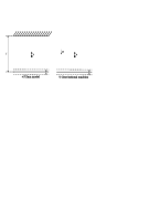
Fig. 1:

The Hamiltonian speed-up model began to be discussed in the physical literature in connection with the prediction of Fermi’s acceleration [26] in the Ulam model [62]. We recall that in this model the particle (in the absence of a gravitational field) is located between two walls, with the lower wall moving periodically in the vertical direction (see Fig. 1$a$). This problem reduces to investigating an area-preserving two-dimensional Poincaré point map. As shown numerically in [62] and then proved analytically in [65, 17, 51], acceleration in different variations of the Ulam model is prevented by an invariant curve existing at large velocities and predicted by KAM theory (see also [49]).

If we remove the upper wall in the Ulam model and place the system in a gravitational field, then we obtain the so-called gravitational machine (see Fig. 1$b$). In this problem there exist trajectories for which the particle gathers speed without bound. For a particular case of motion of the lower wall, the book [64] proposes the model of some random process for description of the dynamics. Analysis of this process shows that the velocity increases as a function of time $t^{\frac{1}{3}}$. In the general case, the presence of accelerating trajectories is proved by Pustylnikov in [56], where it is also shown that the velocity of the particle at instants of collisions increases as a function of time $t^{\frac{1}{2}}$. Causes of the absence of an invariant curve at large velocities in a gravitational machine are discussed in [50].

Thus, in Hamiltonian systems with one and a half degrees of freedom the problem of acceleration reduces to investigating the conditions under which the KAM curves existing in the general case at large energies are destroyed. Among modifications of the Ulam model in which acceleration is observed, we mention generalizations associated with random [37, 33] and piecewise smooth [21] motion of the wall and a relativistic generalization [57].

Acceleration in (nonlinear) natural Hamiltonian systems for two and a half and more degrees of freedom is closely related to Arnold’s diffusion. A detailed discussion of these issues can be found in [29]. We note that there are already a number of systems in which acceleration is shown numerically [46, 55] or using analytical methods, which make it possible to prove the presence of trajectories with increasing energy [4, 41, 28]. An insightful example, which has been intensively discussed recently, is the two-dimensional periodically pulsating Birkhoff billiard. When pulsation is introduced, different degrees of growth of energy of the particle are possible depending on the shape of the boundary determining the dynamical (stochastic, ergodic or regular) behavior of the “frozen system”. We note that the possibility of speeding up the particle by rotating the billiard is numerically investigated in [20]. It is shown that, if there is a region on the boundary of the billiard in which the curvature changes sign, acceleration is observed.

5. As noted above, nonholonomic systems possess no invariant measure in the general case. Consequently, in the general case, KAM theory cannot be applied to them. This is particularly clearly seen in the problem of the Chaplygin sleigh with periodically changing gyrostatic momentum. It turns out that all solutions of the reduced system are accelerating and have identical asymptotics of the growth of the translational velocity as a function of time $\tau^{\frac{1}{3}}$.

In the gravitational machine it is assumed that the particle collides absolutely elastically with the wall. If one introduces dissipation into this system, assuming the impact to be not absolutely elastic, then acceleration disappears in the gravitational machine [31]. A similar situation is observed in the system considered in this paper. If one introduces the force of viscous friction in the Chaplygin sleigh with variable gyrostatic momentum, then unbounded speed-up disappears also. In this paper we show that all trajectories of the reduced system tend to a limit cycle.

The problem dealt with in this paper shows that in nonholonomic mechanics acceleration is characteristic even of small dimensions. We mention the recent paper [1], in which the speed-up of the Chaplygin sleigh is studied using the averaging method and the asymptotics of the degree of speed-up as a function of time is obtained. We note that the absence of an invariant measure turns out to be essential and necessary for the presence of speed-up. These issues are very important for developing the control of various mechanical devices.

The problem we consider here is a model problem, but its analysis allows one to pose the problem of the possibility of speed-up in nonholonomic robots with a more complex control mechanism. In particular, the control of spherical robots is discussed in [40, 8, 9]. The investigation of speed-up in such systems is a complicated and interesting problem.

In conclusion, we note that the Hamiltonian modification of the Chaplygin sleigh (the vakonomic sleigh) can be implemented by means of a plate moving in a fluid. If the mass distribution of the plate depends on time, then the problem reduces to investigating the Hamiltonian system with one and a half degrees of freedom. In this case, it turns out impossible to speed up the plate indefinitely by periodically changing the gyrostatic momentum. This is prevented by an invariant curve existing at large velocities of motion [16].

1 Equations of motion

The Chaplygin sleigh is a platform (rigid body) moving on a horizontal plane with a nonholonomic constraint: at some point the velocity is always orthogonal to a fixed direction. This constraint can be obtained by means of a knife edge rigidly attached to the platform [19] or by means of a wheel pair [7].

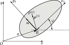
Fig. 2: The Chaplygin sleigh with moving points.

To describe the motion of the sleigh, we define two coordinate systems:

• a fixed (inertial) coordinate system $Oxy$;

• a moving coordinate system $Rx_{1}y_{1}$ attached to the platform.

We specify the position of the sleigh by the coordinates $(x,y)$ of point $R$ in the fixed coordinate system $Oxy$, and the orientation by the rotation angle $\varphi$. Thus, the configuration space of the system $\mathcal{N}=\{\boldsymbol{q}=(x,y,\varphi)\}$ coincides with the motion group of the plane $SE(2)$.

Let $\boldsymbol{v}=(v_{1},v_{2})$ denote the projections of the velocity of point $R$ relative to the fixed coordinate system $Oxy$ onto the moving axes $Rx_{1}y_{1}$ and let $\omega$ be the angular velocity of the body. Then

$$\dot{x}=v_{1}\cos\varphi-v_{2}\sin\varphi,\quad\dot{y}=v_{1}\sin\varphi+v_{2}\cos\varphi,\quad\dot{\varphi}=\omega.$$ (1.1)

The constraint equation in this case reads

$$v_{2}=0.$$ (1.2)

Suppose that $n$ material points $P^{(i)}$, $i=1,..,n$ move on the platform in a prescribed manner. In this case the kinetic energy of the entire system can be represented in the following form [3]:

$$T=\frac{1}{2}m\boldsymbol{v}^{2}+m\omega(c_{1}(t)v_{2}-c_{2}(t)v_{1})+\frac{1}{2}(I(t)+mc^{2}_{2}(t))\omega^{2}+$$

$$+m\big{(}v_{1}\dot{c}_{1}(t)+v_{2}\dot{c}_{2}(t)\big{)}+k(t)\omega,$$

where $m$ is the mass of the entire system, $I(t)$ is its moment of inertia, $\boldsymbol{c}=(c_{1}(t),c_{2}(t))$ is the position of the center of mass, and $k(t)$ is the gyrostatic momentum arising from the motion of the points.

For this system the Lagrange equations with undetermined multipliers have the form

$$\begin{array}[]{ll}\displaystyle\frac{d}{dt}\left(\frac{\partial T}{\partial\omega}\right)=v_{2}\frac{\partial T}{\partial v_{1}}-v_{1}\frac{\partial T}{\partial v_{2}},\quad\displaystyle\frac{d}{dt}\left(\frac{\partial T}{\partial v_{1}}\right)=\omega\frac{\partial T}{\partial v_{2}},\\[11.38109pt] \displaystyle\frac{d}{dt}\left(\frac{\partial T}{\partial v_{2}}\right)=-\omega\frac{\partial T}{\partial v_{1}}+N,\end{array}$$ (1.3)

where $N$ is an undetermined multiplier which is the reaction force at the point of contact $R$. This force is directed transversely to the plane of the knife edge.

In this case it is more convenient to represent this system in the variables $(p,\omega)$, where $p$ is the momentum given by the relation

$$p=\left.\frac{\partial T}{\partial v_{1}}\right|_{v_{2}=0}=m\Big{(}v_{1}-c_{2}(t)\omega+\dot{c}_{1}(t)\Big{)}.$$

From the last equation of (1.3) we find an expression for the reaction force:

$$\begin{array}[]{ll}N=\left(1-\frac{mc_{1}^{2}(t)}{I(t)}\right)\omega p+\left(\dot{c}_{1}(t)-\frac{c_{1}(t)}{I(t)}\big{(}\dot{I}(t)-mc_{1}(t)\dot{c}_{1}\big{)}\right)m\omega-\\[8.53581pt] \displaystyle-\frac{mc_{1}(t)}{I(t)}\left(mc_{2}(t)\ddot{c}_{1}(t)+\dot{k}(t)\right)+m\ddot{c}_{2}(t).\end{array}$$ (1.4)

Finally, from (1.1) and (1.3) we obtain equations of motion in the following form:

$$\begin{array}[]{ll}\dot{p}=mc_{1}(t)\omega^{2}+m\omega\dot{c}_{2}(t),\\[5.69054pt] I(t)\dot{\omega}=-c_{1}(t)\omega p-\big{(}\dot{I}(t)-mc_{1}(t)\dot{c}_{1}(t)\big{)}\omega-mc_{2}(t)\ddot{c}_{1}(t)-\dot{k}(t),\\[5.69054pt] \dot{\varphi}=\omega,\quad m\dot{x}=\big{(}p+c_{2}(t)\omega-\dot{c}_{1}(t)\big{)}\cos\varphi,\quad m\dot{y}=(p+c_{2}(t)\omega-\dot{c}_{1}(t))\sin\varphi.\end{array}$$ (1.5)

In (1.5), the nonautonomous reduced system governing the evolution of $(p,\omega)$ can be considered as a separate set. Of great interest is the question of whether this system has trajectories unbounded on the plane $(p,\omega)$. In this case the sleigh is observed to accelerate, that is, the kinetic energy and hence the velocity of the platform must increase indefinitely with time.

As for acceleration of the sleigh, one should distinguish between cases where the reaction force $N$ is a bounded and an unbounded function of time. Physically, unbounded increase in the reaction force $N$ implies that, at a certain instant of time, slipping will start in the direction transverse to the plane of the knife edge (i.e., the constraint (1.2) will be violated).

What is of interest from a practical point of view is acceleration for which the reaction force $N$ is a bounded function of time.

We consider separately several particular cases where the position of the center of mass $\boldsymbol{c}(t)$, the moment of inertia $I(t)$ and the gyrostatic momentum $k(t)$ depend on time.

Balanced case. If the system is balanced relative to the knife edge $c_{1}=0$ (i.e., the center of mass of the system lies on the axis $Ry_{1}$), then the reduced system reduces to a linear one. In this case the equations of motion possess an additional integral [3]:

$$F=I(t)\omega+k(t).$$ (1.6)

If we fix the level set of the integral $F=f$, then the equation describing the momentum can be represented as

$$\dot{p}=\frac{m\dot{c}_{2}(t)}{I(t)}\big{(}f-k(t)\big{)}.$$

In [3], attention is given to the case in which the functions $I(t)$, $k(t)$, $c_{2}(t)$ periodically depend on time. Then, according to (1.6), the angular velocity $\omega$ is also a periodic function of time, and momentum $p$ depends periodically on time or grows linearly with time. In the latter case, acceleration is observed and, as follows from (1.6), the reaction force $N$ is an unbounded function of time. Moreover, as numerical experiments show, the trajectory of the point of contact in this case has no directed motion [3].

Transverse oscillations. In [3, 1], a detailed analysis is made of the case in which the center of mass of the platform (point $C$) lies in the plane of the knife edge and the material point executes oscillations transverse to this plane (see Fig. 3). Its position in the moving coordinate system $Rx_{1}y_{1}$ is defined by the radius vector

$$\boldsymbol{\rho}=\big{(}a,b\sin(\Omega t)\big{)}.$$

In this case we obtain

$$\begin{array}[]{ll}I(t)=I_{s}+mb^{2}\mu(1-\mu)\sin^{2}(\Omega t),\quad k(t)=mba\mu\Omega\cos(\Omega t),\\[5.69054pt] c_{1}={\rm const},\quad c_{2}(t)=\mu b\sin(\Omega t),\end{array}$$ (1.7)

where $I_{s}$ is the moment of inertia of the platform and $\mu\in(0,1)$ is the ratio of the mass of the point to that of the entire system.

Fig. 3: The Chaplygin sleigh with transversely oscillating mass.

In this case, the reduced system can be represented as

$$\begin{array}[]{ll}\dot{p}\!=\!mc_{1}\omega^{2}+mb\mu\Omega\cos(\Omega t)\omega,\\[8.53581pt] \displaystyle\dot{\omega}\!\!=\!\!-\frac{c_{1}\omega p+mb^{2}\mu(1-\mu)\Omega\sin(2\Omega t)\omega-mba\mu\Omega^{2}\sin(\Omega t)}{I_{s}+mb^{2}\mu(1-\mu)\sin^{2}(\Omega t)}.\end{array}$$ (1.8)

Consider the quadratic function [3]:

$$F=ac_{1}p^{2}+\big{(}(I_{s}+mb^{2}\mu(1-\mu)\sin^{2}(\Omega t))\omega+mba\mu\Omega\cos(\Omega t)\big{)}^{2}.$$

The derivative of this function along the system (1.8) has the form

$$\dot{F}=-2c_{1}p\omega^{2}\big{(}mb^{2}\mu(1-\mu)\sin^{2}(\Omega t)+I_{s}-mac_{1}\big{)}.$$

The conditions for which $\dot{F}$ in the half-planes $p>0$ and $p<0$ is sign-definite are defined by the following relations:

$$ac_{1}<0,\quad\mbox{or}\quad I_{s}-mac_{1}>0.$$ (1.9)

In [3] it is noted that, for parameters satisfying (1.9), one always observes acceleration during which only momentum $p$ grows indefinitely with time (numerical experiments show that it grows in proportion to $\tau^{\frac{1}{3}}$). The first relation of (1.9) has a clear physical interpretation — the center of mass of the system and the oscillating point lie on different sides from the knife edge.

If relations (1.9) are not satisfied, then one observes chaotic oscillations and multistability for which all trajectories of the reduced system (1.8) are bounded. Also, on the Poincaré map one observes a strange attractor which can coexist with invariant curves.

However, the conclusion on acceleration is not rigorously proved in this case. The question of the behavior of the reaction force $N$ remains also open. In addition, numerical experiments show that the point of contact has directed motion.

A sleigh with a rotor. In this paper we consider the motion of the Chaplygin sleigh only with gyrostatic momentum, that is, $I,c_{1},c_{2}={\rm const}$. In this case, gyrostatic momentum can be generated, for example, by two point masses rotating about the common center (see Fig. 4).

Fig. 4: The Chaplygin sleigh with gyrostatic momentum.

Assuming $c_{1}\neq 0$, we define dimensionless variables and parameters:

$$\begin{array}[]{ll}\alpha=\frac{c_{1}p}{I\Omega},\quad u=\frac{\omega}{\Omega},\quad\tau=\Omega t,\quad X=\frac{x}{c_{1}},\quad Y=\frac{y}{c_{1}},\\ \displaystyle A=\frac{mc_{1}^{2}}{I}\in(0,1),\quad a=\frac{c_{2}}{c_{1}},\quad\lambda=\frac{\dot{k}}{\Omega I},\end{array}$$ (1.10)

where $\Omega$ is some constant that has dimension inverse to time. The equations of motion in terms of these variables become

$$\frac{d\alpha}{d\tau}=Au^{2},\quad\frac{du}{d\tau}=-\alpha u-\lambda(\tau),$$ (1.11)

$$\frac{d\varphi}{d\tau}=u,\quad\frac{dX}{d\tau}=\left(\frac{\alpha}{A}+au\right)\cos\varphi,\quad\frac{dY}{d\tau}=\left(\frac{\alpha}{A}+au\right)\sin\varphi.$$ (1.12)

We represent the relation for the reaction force in dimensionless variables in the form

$$\Lambda=\frac{N}{ma\Omega^{2}}=\left(\frac{1}{A}-1\right)\alpha u-\lambda(\tau).$$

Remark 1.

Let the gyrostatic momentum $k(t)$ and the moment of inertia $I(t)$ depend on time and let the center of mass be fixed, $\boldsymbol{c}={\rm const}$. We show that in this case the reduced system can be represented in the form (1.11), where $A$ is a positive function of time.

Indeed, the reduced system has the form

$$\dot{p}=\frac{mc_{1}}{I(t)^{2}}M^{2},\quad\dot{M}=-\frac{c_{1}}{I(t)}Mp-\dot{k},$$

where $M=I(t)\omega$.

Using the fact that the moment of inertia $I(t)$ is a positive function, we rescale time as

$$\tau=\Omega\int\frac{mc_{1}^{2}}{I(t)}dt$$

and introduce new variables

$$\alpha=\frac{p}{mc_{1}\Omega},\quad u=\frac{M}{mc_{1}^{2}\Omega}.$$

The equations of motion in this case can be represented as

$$\frac{d\alpha}{d\tau}=A(\tau)u^{2},\quad\frac{du}{d\tau}=-\alpha u-\lambda(\tau),$$

$$\lambda(\tau)=\frac{dk}{d\tau},\quad A(\tau)=\frac{mc_{1}^{2}}{I(\tau)}.$$

2 Proof of the existence of nonlinear acceleration

Consider in more detail the question of “constant” acceleration of the sleigh by means of a rotor. This question reduces to investigating the possibility of existence of unbounded trajectories for the reduced system (1.11). We note that parameter $A$ in this system can be eliminated by the transformation

$$\quad u\to\frac{1}{\sqrt{A}}u,\quad\lambda(\tau)\to\frac{1}{\sqrt{A}}\lambda(\tau),$$ (2.1)

after which the equations of motion can be represented as

$$\alpha^{\prime}=u^{2},\quad u^{\prime}=-\alpha u-\lambda(\tau),$$ (2.2)

where the prime denotes the derivative with respect to $\tau$.

The right-hand sides of the system of differential equations (2.2) contain quadratic terms. Solutions of such systems can go to infinity in finite time. The simplest example of a system with this property is $x^{\prime}=x^{2}$, $x\in\mathbb{R}$.

We show that all solutions of the system (2.2) are defined on the whole axis of new time $\mathbb{R}=\{\tau\}$. For this purpose we consider the function

$$V=\frac{1}{2}(u^{2}+\alpha^{2}).$$

By virtue of (2.2) the derivative of this function is

$$V^{\prime}=-u\lambda(\tau).$$

Hence,

$$|V^{\prime}|=|u||\lambda|\leqslant\sqrt{2}\sqrt{V}|\lambda|.$$

Since $V\geqslant 0$ and $\sqrt{V}\geqslant 0$, it follows that

$$|V^{-\frac{1}{2}}V^{\prime}|\leqslant\sqrt{2}|\lambda|,$$

or

$$|2\big{(}V^{\frac{1}{2}}\big{)}^{\prime}|\leqslant\sqrt{2}|\lambda|.$$

Integrating the inequalities

$$-\frac{1}{\sqrt{2}}|\lambda(\tau)|\leqslant-|\big{(}V^{\frac{1}{2}}\big{)}^{\prime}|\leqslant\big{(}V^{\frac{1}{2}}\big{)}^{\prime}\leqslant|\big{(}V^{\frac{1}{2}}\big{)}^{\prime}|\leqslant\frac{1}{\sqrt{2}}|\lambda(\tau)|$$

in the interval from $0$ to $\tau$, we find that

$$|V^{\frac{1}{2}}(\tau)-V^{\frac{1}{2}}(0)|\leqslant\frac{1}{\sqrt{2}}\int_{0}^{\tau}|\lambda(s)|ds.$$

Consequently, the function $V(\tau)$ (along with the function $\alpha(\tau)$ and $u(\tau)$) can tend to $+\infty$ only as $|\tau|\to\infty$, which is the required result.

Theorem 1.

Assume that the functions $\lambda(\tau)$ and $\lambda^{\prime}(\tau)$ are bounded and the function $\lambda(\tau)$ does not tend to zero as $\tau\to+\infty$. If at the initial instant of time $\alpha>0$, then for any initial value of the variable $u$

• $\alpha(\tau)$ tends to $+\infty$ as $\tau\to+\infty$,

• $u(\tau)\to 0$ as $\tau\to+\infty$,

• the function $\alpha(\tau)u(\tau)$ is bounded,

• $u^{\prime}(\tau)\to 0$ as $\tau\to+\infty$.

In particular, under these conditions $\alpha^{\prime}(\tau)\to 0$ as $\tau\to+\infty$ and the constraint reaction $\Lambda$ is bounded. The conditions of Theorem 1 for the function $\lambda$ hold if $k(\tau)$ is a periodic or (more generally) conditionally periodic nonconstant function of time.

Proof of Theorem 1.

Conclusion 1 is proved using the following lemma.

Lemma 1 (Hadamard [32]).

If the function $f(\tau)$ tends to the limit as $\tau\to+\infty$ and the functions $f^{\prime}(\tau)$ and $f^{\prime\prime}(\tau)$ are bounded, then $f^{\prime}(\tau)\to 0$ as $\tau\to+\infty$.

The monotone growth of the function $\alpha(\tau)$ follows from the fact that the derivative $\alpha^{\prime}$ is positive for $u\neq 0$ and that $u=0$ is not an invariant submanifold of the system (2.2).

Assume that the function $\alpha(\tau)$ is bounded. Then

$$\lim\limits_{\tau\to\infty}\alpha(\tau)=\bar{\alpha}>0.$$

The positiveness of the limit follows from the assumption that $\alpha(0)>0$.

We show that in this case the function $u(\tau)$ is bounded. Indeed, it satisfies the linear differential equation

$$\frac{du}{d\tau}=-\alpha(\tau)u-\lambda(\tau).$$ (2.3)

We solve it by the method of variation of constants. The solution of the homogeneous equation is

$$u=Ce^{-\int\limits_{0}^{\tau}\alpha(s)ds}.$$

Now, assuming $C$ to be a function of $\tau$, we obtain

$$C^{\prime}=-\lambda(\tau)e^{\int\limits_{0}^{\tau}\alpha(s)ds}.$$

Let us introduce a new function $\widetilde{C}$ by the following formula:

$$\widetilde{C}^{\prime}=-\mu e^{\int\limits_{0}^{\tau}\alpha(s)ds},\quad\mu=\sup|\lambda(\tau)|.$$

It is clear that $|\widetilde{C}^{\prime}|\geqslant|C^{\prime}|$. Consequently, if $C(0)=\widetilde{C}(0)$, then

$$|C(\tau)|\leqslant|\widetilde{C}(\tau)|$$ (2.4)

for all $\tau\geqslant 0$.

Let us calculate

$$\lim\limits_{\tau\to+\infty}\widetilde{C}(\tau)e^{-\int\limits_{0}^{\tau}\alpha(s)ds}=\lim\limits_{\tau\to+\infty}\frac{\widetilde{C}(\tau)}{e^{\int\limits_{0}^{\tau}\alpha(s)ds}}.$$

Since $\alpha(s)\to\bar{\alpha}>0$, the denominator of this fraction tends to $+\infty$ (as does the absolute value of the numerator). Therefore, one can use L’Hôpital’s rule: this limit is

$$\lim\limits_{\tau\to+\infty}\frac{\widetilde{C}^{\prime}}{\alpha(\tau)e^{\int\limits_{0}^{\tau}\alpha(s)ds}}=-\frac{\mu}{\bar{\alpha}}.$$

Thus (according to (2.4)), the function $|u(\tau)|=\Big{|}C(\tau)e^{-\int\limits_{0}^{\tau}\alpha(s)ds}\Big{|}\leqslant\Big{|}\widetilde{C}(\tau)e^{-\int\limits_{0}^{\tau}\alpha(s)ds}\Big{|}$ is bounded.

Further, according to (2.2),

$$\alpha^{\prime\prime}=2uu^{\prime}=-2\alpha u^{2}-2u\lambda(\tau)$$

is also bounded. Therefore (by Hadamard’s lemma), $\alpha^{\prime}(\tau)\to 0$. But then (according to (2.2)) $u(\tau)\to 0$ as $\tau\to+\infty$.

We now consider the second derivative

$$u^{\prime\prime}=-\alpha^{\prime}u-\alpha u^{\prime}+\lambda^{\prime}(\tau).$$

This derivative is bounded since (according to (2.2)) $u^{\prime}$ is bounded. Since  $\!u(\tau)\to 0$ and the derivatives $u^{\prime}(\tau)$ and $u^{\prime\prime}(\tau)$ are bounded,(again according to Hadamard’s lemma) $u^{\prime}(\tau)\to 0$ as $\tau\to+\infty$. But this contradicts the second equation of (2.2), since $\alpha(\tau)\to\bar{\alpha}$ (by assumption), $u(\tau)\to 0$, and the function $\lambda(\tau)$ does not tend to zero as $\tau\to+\infty$.

The resulting contradiction proves conclusion 1. Next, the following lemma is needed.

Lemma 2.

Under the conditions of Theorem 1 the relation

$$\frac{\int\limits_{0}^{\tau}f(p)dp}{f(\tau)},\quad{\rm where}\quad f(p)=e^{\int\limits_{0}^{p}\alpha(s)ds},$$ (2.5)

tends to zero as $\tau\to+\infty$.

Proof.

Since the denominator of (2.5) tends to infinity as $\tau\to+\infty$, one can use L’Hôpital’s rule and the statement (already proved) that $\alpha(\tau)\to+\infty$ as $\tau\to+\infty$. ∎

We now prove conclusion 2. The function $u(\tau)$ as a solution of the linear inhomogeneous differential equation

$$u^{\prime}=-\alpha(\tau)u-\lambda(\tau)$$

is the sum of two functions

$$u(0)e^{-\int\limits_{0}^{\tau}\alpha(s)ds}$$ (2.6)

and

$$-e^{-\int\limits_{0}^{\tau}\alpha(s)ds}\int\limits_{0}^{\tau}\lambda(p)e^{\int\limits_{0}^{p}\alpha(s)ds}dp.$$ (2.7)

The function (2.6) tends superexponentially fast to zero as $\tau\to+\infty$. Since $\lambda(\tau)$ is bounded, the function (2.7) also tends to zero according to Lemma 2.

To prove conclusion 3, we make use of formulae (2.6) and (2.7), the sum of which is the function $u(\tau)$. The product of $\alpha(\tau)$ and the function (2.6) tends to zero as $\tau\to+\infty$. Indeed, according to L’Hôpital’s rule, the limit of this product is equal to

$$u(0)\lim\limits_{\tau\to+\infty}\frac{\alpha^{\prime}(\tau)}{\alpha(\tau)e^{\int\limits_{0}^{\tau}\alpha(s)ds}}=0,$$

since $\alpha^{\prime}(\tau)\to 0$ (according to conclusion 2) and $\alpha(\tau)\to\infty$ as $\tau\to+\infty$.

Since the function $\lambda(\tau)$ is bounded, the product of $\alpha(\tau)$ and the function (2.7) is estimated from above by the function

$$\frac{\alpha(\tau)\int\limits_{0}^{\tau}f(p)dp}{f(\tau)},\quad{\rm where}\quad f(p)=e^{\int\limits_{0}^{p}\alpha(s)ds}.$$

According to L’Hôpital’s rule, the limit of this function as $\tau\to+\infty$ is equal to

$$\lim\limits_{\tau\to+\infty}\frac{\alpha^{\prime}\int\limits_{0}^{\tau}f(p)dp+\alpha(\tau)f(\tau)}{\alpha(\tau)f(\tau)}=1$$

(by Lemma 2). Consequently, the product $\alpha(\tau)u(\tau)$ is indeed bounded.

According to the second equation of (2.2), the derivative $u^{\prime}(\tau)$ is bounded. We prove that $u^{\prime}(\tau)\to 0$ as $\tau\to+\infty$.

Indeed, according to (2.6) and (2.7),

$$-u^{\prime}=\alpha u+\lambda=\frac{\alpha\Big{[}u(0)-\int\limits_{0}^{\tau}\lambda(p)f(p)dp\Big{]}+\lambda(\tau)f(\tau)}{f(\tau)},$$ (2.8)

where $f$ is given by formula (2.5). It is clear that

$$u(0)\frac{\alpha(\tau)}{f(\tau)}\to 0$$

as $\tau\to+\infty$. We calculate the limit of the two remaining terms in (2.8) again by L’Hôpital’s rule. It is equal to

$$\lim\limits_{\tau\to+\infty}\frac{-\alpha^{\prime}\int\limits_{0}^{\tau}\lambda fdp+\lambda^{\prime}f}{\alpha f}.$$ (2.9)

Taking into account the assumption about boundedness of the functions $\lambda(\tau)$ and $\lambda^{\prime}(\tau)$, as well as the already established properties $\alpha(\tau)\to+\infty$, $\alpha^{\prime}(\tau)\to 0$ and Lemma 2, we find that the limit (2.9) is zero. This proves conclusion 4.

∎

Theorem 2.

Suppose that the conditions of Theorem 1 hold and there exists the average

$$\langle\lambda^{2}\rangle=\lim\limits_{\tau\to+\infty}\frac{1}{\tau}\int\limits_{0}^{\tau}\lambda^{2}(p)dp.$$ (2.10)

Then, as $\tau\to+\infty$,

$$\frac{\alpha^{3}(\tau)}{3}=\langle\lambda^{2}\rangle\tau+o(\tau).$$ (2.11)

The average value of (2.10) exists if $\lambda$ is a periodic or conditionally periodic function of time. If $\lambda$ does not vanish, then, obviously, $\langle\lambda^{2}\rangle$ is positive. Formula (2.11) can be represented in the following equivalent form:

$$\alpha=\sqrt[3]{3\langle\lambda^{2}\rangle}\tau^{\frac{1}{3}}+o\Big{(}\tau^{\frac{1}{3}}\Big{)}.$$

Proof of Theorem 2.

Since $u^{\prime}(\tau)\to 0$ as $\tau\to+\infty$ (conclusion 4 of Theorem 1), according to the second equation of (2.2) we have

$$\alpha u=-\lambda(\tau)+f(\tau),$$

where $f(\tau)=o(1)$. Hence,

$$u=\frac{-\lambda+f}{\alpha}.$$

Since $\alpha^{\prime}=u^{2}$, it follows that

$$\Big{[}\frac{1}{3}\alpha^{3}\Big{]}^{\prime}=\lambda^{2}-2\lambda f+f^{2}.$$ (2.12)

Let $g(\tau)$ be one of the functions

$$-2\lambda(\tau)f(\tau)\quad{\rm or}\quad f^{2}(\tau).$$

It is clear that $g(\tau)\to 0$ as $\tau\to+\infty$. Consequently,

$$\int\limits_{0}^{\tau}g(s)ds=o(s).$$

Indeed, since $g(\tau)=o(1)$, we have

$$\lim\limits_{\tau\to+\infty}\frac{1}{\tau}\int\limits_{0}^{\tau}g(s)ds=0.$$

Integrating (2.12), we obtain the required formula:

$$\frac{\alpha^{3}}{3}=\langle\lambda^{2}\rangle\tau+o(\tau).$$

Theorem 3.

Suppose that the conditions of Theorem 1 hold, $u(0)=0$ and the analytic function $k(\tau)$ is such that for any $a>0$ one can find the root of the equation

$$k(\tau)=k(a),$$

which is strictly larger than $a$. Then the function $u(\tau)$ has infinitely many zeros as $\tau\to+\infty$.

Proof of Theorem 3 uses the formula

$$u(\tau)=-\frac{1}{f(\tau)}\int\limits_{0}^{\tau}\lambda(p)f(p)dp,$$ (2.13)

and the property of strict monotone growth of the function $f$. The infinity of the number of zeros of the function (2.13) follows from the following general result [42, Sec. 6].

Lemma 3.

Let $\tau_{1}$ be the first positive zero of the analytic function

$$\int\limits_{a}^{\tau}\lambda(t)dt$$ (2.14)

and let $f$ be a positive nondecreasing function. Then the integral

$$\int\limits_{a}^{\tau}\lambda(t)f(t)dt$$

vanishes on the interval $(a,\tau_{1}]$.

In our case, in view of (1.10) and (2.1), the integral (2.14) is

$$B(k(\tau)-k(a)),\quad B=\frac{1}{\sqrt{A}I\Omega},$$

and therefore the conclusion of Theorem 3 follows from formula (2.13) and Lemma 3.

Corollary 1.

Suppose that the conditions of Theorem 1 hold, $u(0)=0$, and the analytic function $k(\tau)$ is periodic with period $T$. Then the function $u(\tau)$ has infinitely many zeros as $\tau\to+\infty$, and the distance between its neighboring zeros does not exceed $T$.

3 Dynamics in configuration space

As shown in the previous section for solutions to the reduced system, in view of the transformation (2.1) we have

$$\begin{array}[]{ll}\alpha(\tau)=\sigma\tau^{\frac{1}{3}}+o(\tau^{\frac{1}{3}}),\qquad u(\tau)=-\frac{\lambda(\tau)}{\sigma}\tau^{-\frac{1}{3}}+o(\tau^{-\frac{1}{3}}),\\ \sigma=\left(3A\langle\lambda^{2}\rangle\right)^{\frac{1}{3}},\end{array}$$ (3.1)

where $\langle\lambda^{2}\rangle$ is defined by (2.10).

From the given solutions of the reduced system the orientation of the Chaplygin sleigh and the motion of the point of contact are defined by quadratures (1.12). If we restrict ourselves to the asymptotics (3.1), we obtain

$$\begin{array}[]{ll}\displaystyle\frac{d\varphi}{d\tau}=-\frac{\lambda(\tau)}{\sigma}\tau^{-\frac{1}{3}},\\[11.38109pt] \displaystyle\frac{dX}{d\tau}=\frac{\sigma}{A}\tau^{\frac{1}{3}}\cos\varphi,\quad\displaystyle\frac{dY}{d\tau}=\frac{\sigma}{A}\tau^{\frac{1}{3}}\sin\varphi.\end{array}$$ (3.2)

We let $\tau=\tau_{0}>0$ denote time from which the asymptotics (3.1) describes “well” the solution of the reduced system, and supplement the system (3.2) with the following initial conditions:

$$\varphi(\tau_{0})=X_{0},\quad X(\tau_{0})=Y_{0},\quad Y(\tau_{0})=Z_{0}.$$ (3.3)

Consider the system (3.2) in more detail in two cases:

• constantly accelerating rotor — the angular velocity of the rotor is a linear function of time, in this case $\lambda(\tau)=\lambda_{0}={\rm const}$;

• periodically oscillating rotor — the angular velocity of the rotor is a periodic function of time. As an example we consider the function $\lambda(\tau)=\lambda_{0}\sin\tau$.

Constantly accelerating rotor ($\lambda(\tau)=\lambda_{0}>0$). Explicitly integrating the system (3.2), we find

$$\varphi(\tau)=-s_{1}(\tau^{\frac{2}{3}}-\tau_{0}^{\frac{2}{3}})+\varphi_{0},\quad s_{1}=\left(\frac{9\lambda_{0}}{8A}\right)^{\frac{1}{3}},$$ (3.4)

$$\begin{array}[]{ll}X(\tau)=2\big{(}\cos\varphi(\tau)-s_{1}\tau^{\frac{2}{3}}\sin\varphi(\tau)\big{)}-2\big{(}\cos\varphi_{0}-s_{1}\tau_{0}^{\frac{2}{3}}\sin\varphi_{0}\big{)}+X_{0},\\[5.69054pt] Y(\tau)=2\big{(}\sin\varphi(\tau)+s_{1}\tau^{\frac{2}{3}}\cos\varphi(\tau)\big{)}-2\big{(}\sin\varphi_{0}+s_{1}\tau_{0}^{\frac{2}{3}}\cos\varphi_{0}\big{)}+Y_{0}.\end{array}$$ (3.5)

As we see, the trajectory of the point of contact is an untwisting spiral (Fig. 5) and in this case there is no directed motion of the sleigh.

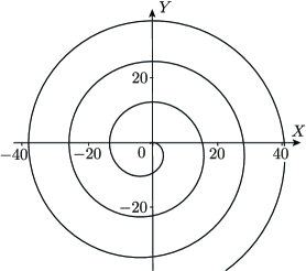
Fig. 5: The curve (3.5) with fixed $A=1$, $\lambda_{0}=1$, $\varphi_{0}=0$, $X_{0}=0$, $Y_{0}=0$, $\tau_{0}=1$.

Periodically oscillating rotor ($\lambda(\tau)=\lambda_{0}\sin\tau$). A typical behavior of the solutions to the system (1.11) and (1.12) in this case is presented in Fig. 6. As numerical experiments show, the following statement holds.

In the case of a periodically oscillating rotor the angle of rotation of the sleigh $\varphi$ tends to a finite limit, and the “limit” motions of the point of contact are oscillations (with constant amplitude) in a neighborhood of a straight line.

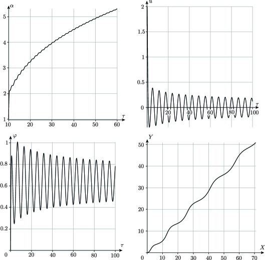
Fig. 6: Functions $\alpha(\tau)$, $u(\tau)$, $\varphi(\tau)$, $Y(X)$ plotted numerically for fixed parameters $\lambda_{0}=1$, $A=1$ and initial conditions $\tau=0$, $\alpha=1$, $u=2$, $\varphi=0$, $X=0$, $Y=0$.

In order to show the validity of this statement, we consider the system (3.2) in the approximation (3.1) and make use of the relation [54, p.401]

$$\int_{\tau}^{\infty}\frac{\sin\xi}{\xi^{\frac{1}{3}}}d\xi=\frac{\cos\tau}{\tau^{\frac{1}{2}}}+O(\tau^{-\frac{4}{3}}).$$

This yields

$$\varphi(\tau)=\widetilde{\varphi}+s_{2}\frac{\cos\tau}{\tau^{\frac{1}{3}}}+O(\tau^{-\frac{4}{3}}),\quad s_{2}=\left(\frac{2\lambda_{0}}{3A}\right)^{\frac{1}{3}},$$

$$\widetilde{\varphi}=\varphi_{0}-s_{2}\frac{\cos\tau_{0}}{\tau_{0}^{\frac{1}{3}}}+O(\tau_{0}^{-\frac{4}{3}}),$$

that is, the angle of rotation of the sleigh tends to a fixed value of $\widetilde{\varphi}$ as $t\to+\infty$. We substitute the function $\varphi(\tau)$ obtained into the equations for the evolution of the point of contact and expand the resulting expressions in powers of $\tau^{-\frac{1}{3}}$. Neglecting terms of order $O(\tau^{-\frac{4}{3}})$ and $O(\tau_{0}^{-\frac{4}{3}})$, we represent the equations of motion for the point of contact in the form

$$\begin{array}[]{ll}\displaystyle\frac{dX}{d\tau}=\frac{\sigma}{A}\left(\tau^{\frac{1}{3}}\cos\widetilde{\varphi}+s_{2}\cos\tau\sin\widetilde{\varphi}\right),\\[8.53581pt] \displaystyle\frac{dY}{d\tau}=\frac{\sigma}{A}\left(\tau^{\frac{1}{3}}\sin\widetilde{\varphi}-s_{2}\cos\tau\cos\widetilde{\varphi}\right).\end{array}$$

If we rotate the fixed coordinate system through angle $\widetilde{\varphi}$:

$$\widetilde{X}=X\cos\widetilde{\varphi}+Y\sin\widetilde{\varphi},\quad\widetilde{Y}=-X\sin\widetilde{\varphi}+Y\cos\widetilde{\varphi},$$

then the equations of motion become

$$\frac{d\widetilde{X}}{d\tau}=\frac{\sigma}{A}\tau^{\frac{1}{3}},\quad\frac{d\widetilde{Y}}{d\tau}=-s_{2}\frac{\sigma}{A}\cos\tau.$$

Explicitly integrating this system, we find

$$\begin{array}[]{ll}\displaystyle\widetilde{X}(\tau)=\widetilde{X}_{0}+\frac{3}{4}\frac{\sigma}{A}(\tau^{\frac{4}{3}}-\tau_{0}^{\frac{4}{3}}),\\[8.53581pt] \displaystyle\widetilde{Y}(\tau)=\widetilde{Y}_{0}-\frac{\sigma}{A}s_{2}(\sin\tau-\sin\tau_{0}),\end{array}$$ (3.6)

where $\widetilde{X}_{0}$ and $\widetilde{Y}_{0}$ are initial conditions calculated using (3.3). Thus, along the axis $\widetilde{X}$ the sleigh moves away in proportion to $\tau^{\frac{4}{3}}$, and along the axis $\widetilde{Y}$ it executes oscillations with constant amplitude $\displaystyle\frac{\sigma s_{2}}{A}=\frac{\lambda_{0}}{A}$.

Let us compare relation (3.6) with the numerical solution of the system (1.11)–(1.12). To do so, we calculate the angle:

$$\begin{array}[]{ll}\displaystyle\tilde{\varphi}_{n}=\frac{\psi_{1}+\psi_{2}}{2},\quad\psi_{1}=\frac{1}{2\pi}\int\limits_{\tau_{0}}^{\tau_{0}+2\pi n}\varphi(\tau)d\tau,\\[8.53581pt] \displaystyle\psi_{2}=\frac{1}{2\pi}\int\limits_{\tau_{0}+\pi}^{\tau_{0}+\pi(2n+1)}\varphi(\tau)d\tau,\quad n\in\mathbb{N},\end{array}$$ (3.7)

where the function $\varphi(\tau)$ is a numerical solution of the initial system. The angle of rotation is defined by

$$\tilde{\varphi}=\lim\limits_{n\to\infty}\varphi_{n},$$

that is, the larger $n$, the more exactly $\varphi_{n}$ approximates $\tilde{\varphi}$.

A typical view of the trajectory of the point of contact is shown in Fig. 7. As we see, the relation obtained for the amplitude agrees well with the numerical experiments. However, a rigorous proof of this fact requires investigating more detailed estimates for the functions $\alpha(\tau)$ and $u(\tau)$ (than that considered in this section (3.1)).

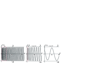
Fig. 7: Trajectory of the point of contact plotted numerically for fixed parameters $\lambda_{0}=1$, $A=1$ and initial conditions $\tau=0$, $\alpha=0$, $u=0$, $\varphi=0$, $X=0$, $Y=0$. In this case $\tilde{\varphi}=4.638$ ($n=10$) and $\tilde{Y}_{0}=-1.068$.

4 Viscous friction

We assume that the motion of the sleigh occurs in the presence of viscous friction force with a dissipative Rayleigh function of the form

$$F=\frac{1}{2}\big{(}\nu_{1}v_{1}^{2}+\nu_{2}\omega^{2}\big{)}.$$

For the system of Lagrange equations with undetermined multipliers we write

$$\begin{array}[]{ll}\displaystyle\frac{d}{dt}\left(\frac{\partial T}{\partial v_{1}}\right)=\omega\frac{\partial T}{\partial v_{2}}-\nu v_{1},&\displaystyle\frac{d}{dt}\left(\frac{\partial T}{\partial\omega}\right)=v_{2}\frac{\partial T}{\partial v_{1}}-v_{1}\frac{\partial T}{\partial v_{2}}-\nu_{2}\omega,\\[11.38109pt] \displaystyle\frac{d}{dt}\left(\frac{\partial T}{\partial v_{2}}\right)=-\omega\frac{\partial T}{\partial v_{1}}+N.\end{array}$$

In the presence of friction force the reduced system can be reduced, after a transformation similar to (2.1), to the form

$$\begin{array}[]{l}\alpha^{\prime}=Au^{2}-\sigma_{1}\alpha,\quad u^{\prime}=-\alpha u-\lambda(\tau)-\sigma_{2}u,\\[8.53581pt] \displaystyle\frac{d\varphi}{d\tau}=u,\quad\frac{dX}{d\tau}=\left(\frac{\alpha}{A}+au\right)\cos\varphi,\quad\frac{dY}{d\tau}=\left(\frac{\alpha}{A}+au\right)\sin\varphi,\end{array}$$ (4.1)

where $\sigma_{1}$ and $\sigma_{2}$ are the coefficients of friction. As numerical experiments show (see Fig. 8), there is no acceleration in (4.1) in this case.

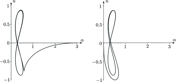
Fig. 8: A typical view of a periodic solution and of trajectories tending to it for the system (4.2) with $\lambda(\tau)=\sin\tau$, $\mu=0.3$.

Let us perform normalizing transformations of the variables, functions and time

$$\alpha\to\sigma_{1}\alpha,\quad u\to\frac{\sigma_{1}}{\sqrt{A}}u$$

$$\lambda\to\frac{\sigma_{1}^{2}}{\sqrt{A}}\lambda,\quad\sigma_{2}\to\sigma_{1}\mu,\quad\sigma_{1}d\tau\to d\tau,$$

and represent the system as

$$\alpha^{\prime}=u^{2}-\alpha,\quad u^{\prime}=-\alpha u-\lambda(\tau)-\mu u.$$ (4.2)

We now apply the Brower theorem to this system (see Appendix ). To do so, we consider a closed region $\mathcal{D}_{\mu,\lambda_{m}}$ on the plane $(\alpha,u)$ bounded by four straight lines (see Fig. 9)

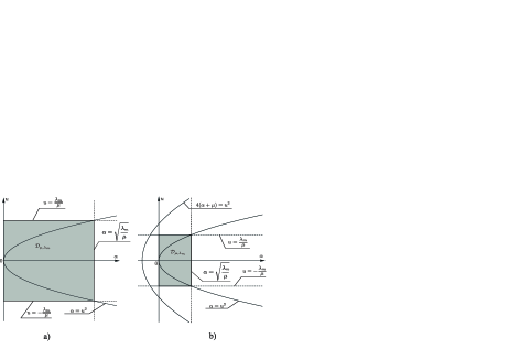
Fig. 9:

$$\begin{array}[]{ll}\displaystyle\gamma_{1}:\alpha=0,\quad\gamma_{2}:\alpha=\sqrt{\frac{\lambda_{m}}{\mu}},\\[11.38109pt] \displaystyle\gamma_{3}:u=\frac{\lambda_{m}}{\mu},\quad\gamma_{4}:u=-\frac{\lambda_{m}}{\mu},\end{array}$$ (4.3)

where $\lambda_{m}=\max|\lambda(\tau)|$.

We show that this region is invariant under the flow. Indeed, according to the second equation in (4.2), the vector field on the curves $\gamma_{3}$ and $\gamma_{4}$ is directed into the region $\mathcal{D}_{\mu,\lambda_{m}}$ (since the inequalities $\dot{u}\leqslant 0$ and $\dot{u}\geqslant 0$ are satisfied for all $t$ on the upper straight line $\gamma_{3}$ and on the lower straight line $\gamma_{4}$, respectively). Similarly, on the straight line $\gamma_{1}$ the vector field is also directed into the region (since on this straight line $\dot{\alpha}\geqslant 0$), on the other hand, on the straight line $\gamma_{2}$ the vector field is also directed inside (since the segment under consideration gets into the parabola $\alpha=u^{2}$, where $\dot{\alpha}\leqslant 0$).

Hence, on the basis of Theorem A.1 of Appendix we obtain the following theorem.

Theorem 4.

In the system $(\ref{2812})$ with $\mu\neq 0$ there exists at least one periodic solution in the region $\mathcal{D}_{\mu,\lambda_{m}}$.

Now, in order to clarify the conditions for uniqueness of the periodic solution in the region $\mathcal{D}_{\mu,\lambda_{m}}$, we find a region on the plane $(\alpha,u)$ where the map for a period of the system (4.2) is compressing. According to Appendix , this requires ascertaining the region of negative definiteness of the symmetric part of the Jacobian of the right-hand side of the system (4.2):

$$\begin{array}[]{cc}{\bf B}=\left(\begin{array}[]{cc}-1&\frac{u}{2}\\ \frac{u}{2}&-\alpha-\mu\end{array}\right).\end{array}$$

Its eigenvalues $b_{\pm}$ are given by

$$b_{\pm}=-\frac{1}{2}\big{(}\alpha+\mu+1\pm\sqrt{u^{2}+(\alpha+\mu-1)^{2}}\big{)}.$$

We thus find that the “compression region” (i. e., the region where $b_{\pm}<0$) is given by

$$4(\alpha+\mu)\geqslant u^{2}.$$

Using the equations of the upper and lower boundaries (4.3) of the region $\mathcal{D}_{\mu,\lambda_{m}}$, we obtain

Theorem 5.

If in the system (4.2)

$$2\mu^{3/2}\geqslant\lambda_{m},$$ (4.4)

then in the region $\mathcal{D}_{\mu,\lambda_{m}}$ there exists the only periodic orbit to which all other trajectories in $\mathcal{D}_{\mu,\lambda_{m}}$ tend exponentially.

We note that in this section we obtain an estimate of the region of existence of the limit cycle $\mathcal{D}_{\mu,\lambda_{m}}$ from the point of view of its localization. Generally speaking, one can pose the problem of more exact localization of the limit cycle, that is, the problem of finding the smallest possible region $\mathcal{D}^{\prime}\subset\mathcal{D}_{\mu,\lambda_{m}}$ containing this cycle. On the other hand, under the conditions of Theorem 5 one can also pose the problem of finding the largest possible region $\mathcal{D}^{\prime\prime}\supset\mathcal{D}_{\mu,\lambda_{m}}$ in which all trajectories tend to the only limit cycle.

The system (4.1) in the case $\sigma_{2}=0$ and $\lambda(\tau)=\sin\tau$ was considered in [25]. In this case, inequality (4.4) does not hold. However, numerical experiments show that Theorem 5 remains valid.

Dynamics in configuration space. A typical behavior of solutions to the system (4.1) is shown in Fig. 10. We see that the “limit” motions of the point of contact, as in the absence of friction force, are oscillations (with constant amplitude) in a neighborhood of a straight line. In this case, in a neighborhood of the limit cycle the rotation angle and the translational and angular velocities of the sleigh change periodically with time (i. e., there is no unbounded increase in the translational velocity).

The trajectory of the point of contact in the variables of Section 3 is presented in Fig. 11. This implies that, as the friction coefficient increases, the oscillation amplitude decreases.

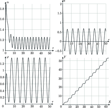
Fig. 10: Functions $\alpha(\tau)$, $u(\tau)$, $\varphi(\tau)$, $Y(X)$ plotted numerically for fixed parameters $\lambda_{0}=1$, $A=1$, $\sigma_{1}=0.1$, $\sigma_{2}=0$ and initial conditions $\tau=0$, $\alpha=1$, $u=2$, $\varphi=0$, $X=0$, $Y=0$.

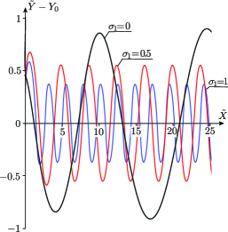
Fig. 11: Trajectory of the point of contact plotted numerically for fixed parameters $\lambda_{0}=1$, $A=1$, $\sigma_{2}=0$ and initial conditions $\tau=0$, $\alpha=0$, $u=0$, $\varphi=0$, $X=0$, $Y=0$ for different $\sigma_{1}$.

5 The problem of acceleration in nonholonomic systems

We discuss a number of problems that can be investigated by the methods presented in this paper. The hydrodynamical model of the Chaplygin sleigh was proposed in [23]. Although this model requires additional justification from the hydrodynamical point of view, it would be interesting to explore a nonautonomous analogue of this model. The same can be said of the problem of a sleigh with a constraint inhomogeneous in the velocities, which has been investigated recently in [13].

Further we consider several systems of nonholonomic mechanics with parametric excitation which is achieved by a given periodic motion of some structural elements. Their common feature is that the system of equations has a subsystem that governs the evolution of (generalized) velocities with coefficients periodically depending on time and can be considered as a separate set (the dimension of this subsystem does not exceed 2).

The simplest case is the Roller Racer [45]. We recall that the Roller Racer consists of two coupled bodies with a pair of wheels attached on each of the bodies (see Fig. 12). The distinctive feature of the Roller Racer is that the user moves forward by oscillating the front handlebars in the transverse direction from side to side. As a rule, when investigating this system one assumes that, as a result of external action, the angle between the two coupled bodies is a given function of time (kinematic control).

Fig. 12:

In this case, one can decouple a linear equation with periodic coefficients which governs the evolution of the translational velocity of one of the bodies:

$$\dot{w}=A(t)w+B(t),\quad A(t)=A(t+T),\quad B(t)=B(t+T).$$ (5.1)

For some particular mass distribution of the coupled bodies equation (5.1) has been obtained in [45], where it is shown that in this case acceleration is observed. However, this has not been rigorously proved as yet.

In a more complicated situation, namely, the Suslov problem with moving masses, we have a special two-dimensional (nonlinear) system that generalizes the system dealt with in this paper:

$$\begin{array}[]{ll}\big{(}{\bf G}(t)\boldsymbol{w}+\boldsymbol{K}(t)\big{)}^{\!\boldsymbol{\cdot}}=\Phi(\boldsymbol{w}){\bf J}\boldsymbol{w},\\[8.53581pt] \boldsymbol{w}=(w_{1},w_{2}),\quad{\bf J}=\left(\begin{array}[]{cc}0&-1\\ 1&0\end{array}\right),\quad{\bf G}(t)={\bf G}^{T}(t)\\[8.53581pt] \Phi(\boldsymbol{w})=a_{1}(t)w_{1}+a_{2}(t)w_{2}+k_{3}(t),\end{array}$$ (5.2)

where all functions of time $T$ are periodic and the symmetric matrix ${\bf G}(t)$ is positive definite for all $t$.

In the case where all coefficients of the system (5.2) are constant, its trajectories on the plane $(w_{1},w_{2})$ are very simple. First, there is an invariant submanifold — the straight line

$$a_{1}w_{1}+a_{2}w_{2}+k_{3}=0,$$ (5.3)

which is filled with fixed points. The other trajectories lie on ellipses which are level lines of the energy integral

$$E=\frac{1}{2}\big{(}\boldsymbol{w},{\bf G}\boldsymbol{w}\big{)}={\rm const}.$$ (5.4)

The level lines (5.4) that intersect the straight line (5.3) consist of two asymptotic trajectories connecting a pair of equilibrium points, whereas the level lines that do not intersect the straight line (5.3) define the periodic orbits of the system (5.2). Moreover, in this case, by a natural linear transformation

$$u=a_{1}w_{1}+a_{2}w_{2},\quad\alpha=A\big{(}(a_{1}G_{12}-a_{2}G_{11})w_{1}+(a_{1}G_{22}-a_{2}G_{12})w_{2}\big{)},\quad A={\rm const}$$

the system (5.2) is brought to the simple form

$$\dot{\alpha}=Au(u+k_{3}),\quad\dot{u}=-\frac{\alpha(u+k_{3})}{A\det{\bf G}}.$$ (5.5)

Appendix A. The principle of compressing maps

1. In this section, we briefly formulate in a form convenient for our purposes some results on the periodic solutions of the system which depend periodically on time. Let the following system be given in the Euclidean space $E^{n}=\big{\{}\boldsymbol{x}=(x_{1},\ldots,x_{n})\big{\}}$:

$$\boldsymbol{\dot{x}}=\boldsymbol{v}(\boldsymbol{x},t),\quad\boldsymbol{v}(\boldsymbol{x},t+T)=\boldsymbol{v}(\boldsymbol{x},t).$$ (A.1)

We first define the notion of an invariant subset $\mathcal{D}\subset\mathcal{M}$.

Definition 1.

If for all initial conditions $t_{0}\in[0,T]$ and $\boldsymbol{x}_{0}\subset\mathcal{D}$ the trajectories $\boldsymbol{x}(t)\subset\mathcal{D}$, $t>t_{0}$, then $\mathcal{D}$ is said to be an invariant subset.

If the vector field (A.1) has no singular points inside $\mathcal{D}$, then a natural family of maps for a period is defined:

$$\Pi_{t_{0}}:\mathcal{D}\to\mathcal{D},$$ (A.2)

which assigns to each point $\boldsymbol{x}_{0}$ point $\boldsymbol{x}$ at time $t_{0}+T$, on the trajectory of the system with initial conditions $\boldsymbol{x}(t_{0})=\boldsymbol{x}_{0}$. The existence and uniqueness theorem and the theorem of continuous dependence on initial conditions guarantee that the maps $\Pi_{t_{0}}$ are continuous and biunique on their image.

If the set $\mathcal{D}$ is homeomorphic to a closed ball, then, according to the Brower theorem, any map (A.2) has a fixed point inside $\mathcal{D}$:

$$\Pi_{t_{0}}(\boldsymbol{x}^{*})=\boldsymbol{x}^{*}.$$

In the flow (A.1) this fixed point corresponds to the periodic solution

$$\boldsymbol{x}_{p}(t)=\boldsymbol{x}_{p}(t+T),\quad\boldsymbol{x}_{p}(t_{0})=\boldsymbol{x}^{*}.$$

Thus, the following theorem holds.

Theorem A.1.

Suppose that the system $(\ref{eqa1})$ admits an invariant set $\mathcal{D}$ that is homeomorphic to a closed ball and does not contain any singular points of the vector field. Then in $\mathcal{D}$ there is at least one periodic solution.

2. Now assume that the flow (A.1) admits a closed invariant set $\mathcal{D}$ inside which it possesses the property of uniform compression, namely: the following inequality is satisfied for any two trajectories $\boldsymbol{x}_{1}(t),\,\boldsymbol{x}_{2}(t)$ inside $\mathcal{D}$ at all instants of time $t$:

$$|\boldsymbol{x}_{1}-\boldsymbol{x}_{2}|^{\boldsymbol{\cdot}}=\frac{\big{(}\boldsymbol{x}_{1}-\boldsymbol{x}_{2},\,\boldsymbol{v}(\boldsymbol{x}_{1},t)-\boldsymbol{v}(\boldsymbol{x}_{2},t)\big{)}}{|\boldsymbol{x}_{1}-\boldsymbol{x}_{2}|}\leqslant-h|\boldsymbol{x}_{1}-\boldsymbol{x}_{2}|,$$ (A.3)

where $h>0$ is some constant.

In this case the maps (A.2) are also compressing

$$|\Pi_{t_{0}}(\boldsymbol{x}_{1})-\Pi_{t_{0}}(\boldsymbol{x}_{2})|\leqslant\lambda|\boldsymbol{x}_{1}-\boldsymbol{x}_{2}|,\quad\lambda=e^{-hT}<1.$$ (A.4)

Indeed, let $\Delta(t)=|\boldsymbol{x}^{(1)}(t)-\boldsymbol{x}^{(2)}(t)|$, where $\boldsymbol{x}^{(k)}(t)$, $k=1,2$ are trajectories of the system (A.1) that satisfy the initial conditions $\boldsymbol{x}^{(k)}(t_{0})=x_{k}$, $k=1,2$. Then $\Delta(t_{0})=|\boldsymbol{x}_{1}-\boldsymbol{x}_{2}|$ and $\Delta(t_{0}+T)=|\Pi_{t_{0}}(\boldsymbol{x}_{1})~{}-~{}\Pi_{t_{0}}(\boldsymbol{x}_{2})|$. From the above inequality (A.3) and the condition $\Delta(t)>0$ we obtain

$$\big{(}\ln\Delta(t)\big{)}^{\boldsymbol{\cdot}}\leqslant-h.$$

Integrating this relation for a period, we obtain (A.4).

Thus, we apply to $\Pi_{t_{0}}$ the principle of compressing Banach maps [66], according to which $\Pi_{t_{0}}$ has a unique fixed point $\boldsymbol{x}^{*}$ in $\mathcal{D}$ to which the trajectory of any other point tends exponentially. Thus, the following theorem holds.

Theorem A.2.

Suppose that the system $(\ref{eqa1})$ possesses the property of uniform compression inside some closed invariant set $\mathcal{D}$. Then in $\mathcal{D}$ there exists a unique periodic solution and all other trajectories in $\mathcal{D}$ tend to it exponentially.

We now give the simplest criterion for uniform compression as presented in [22]. Define the Jacobian of the right-hand side of (A.1):

$${\bf J}(\boldsymbol{x},t)=\bigg{\|}\frac{\partial v_{i}(\boldsymbol{x},t)}{\partial x_{j}}\bigg{\|}.$$

Proposition 1.

([22]) Suppose that the quadratic form given by the matrix $\bf J$ is uniformly negative definite for all $\boldsymbol{x}\in\mathcal{D}$ and $t$:

$$\big{(}\boldsymbol{x},{\bf J}(\boldsymbol{x},t)\boldsymbol{x}\big{)}\leqslant-h(\boldsymbol{x},\boldsymbol{x}),$$

where $h>0$ is some constant. Then the flow of the system possesses the property of uniform compression.

Finally, we obtain the following result.

Theorem A.3.

If the eigenvalues of the matrix

$${\bf B}(\boldsymbol{x},t)=\frac{1}{2}\big{(}{\bf J}(\boldsymbol{x},t)+{\bf J}^{T}(\boldsymbol{x},t)\big{)},\quad\boldsymbol{x}\in\mathcal{D}$$

are negative and separated from zero, then the system $(\ref{eqa1})$ possesses a unique limit cycle in $\mathcal{D}$ to which all other trajectories tend exponentially.

References

- [1] Bizyaev I A, Borisov A V and Kuznetsov S P 2017 Chaplygin sleigh with periodically oscillating internal mass EPL 119 60008
- [2] Bizyaev I A Borisov A V and Mamaev I S 2016 Dynamics of the Chaplygin Sleigh on a Cylinder Regular and Chaotic Dynamics 21 136–146
- [3] Bizyaev I A, Borisov A V and Mamaev I S 2017 The Chaplygin Sleigh with Parametric Excitation: Chaotic Dynamics and Nonholonomic Acceleration Regular and Chaotic Dynamics 22 955–975
- [4] Bolotin S abd Treschev D 1999 Unbounded growth of energy in nonautonomous Hamiltonian systems Nonlinearity 12 365–388
- [5] Borisov A V, Jalnine A Y, Kuznetsov S P, Sataev I R and Sedova Y V 2012 Dynamical Phenomena Occurring due to Phase Volume Compression in Nonholonomic Model of the Rattleback Regul. Chaotic Dyn. 17 512–532
- [6] Borisov A V, Kazakov A O and Sataev I R 2014 The Reversal and Chaotic Attractor in the Nonholonomic Model of Chaplygin s Top Regul. Chaotic Dyn. 19 718–733
- [7] Borisov A V, Kilin A A and Mamaev I S 2015 On the Hadamard – Hamel Problem and the Dynamics of Wheeled Vehicles Regular and Chaotic Dynamics 20 752–766
- [8] Borisov A V, Kilin A A and Mamaev I S 2012 How to Control Chaplygin s Sphere Using Rotors Regular and Chaotic Dynamics 17 258–272
- [9] Borisov A V, Kilin A A and Mamaev I S 2013 How to Control the Chaplygin Ball Using Rotors. II Regular and Chaotic Dynamics 18 144–158
- [10] Borisov A V and Kuznetsov S P 2016 Regular and Chaotic Motions of a Chaplygin Sleigh under Periodic Pulsed Torque Impacts Regular and Chaotic Dynamics 21 792–803
- [11] Borisov A V and Mamaev I S 2009 The dynamics of a Chaplygin sleigh Journal of Applied Mathematics and Mechanics 73 156–161
- [12] Borisov A V and Mamaev I S 2003 Strange Attractors in Rattleback Dynamics Physics-Uspekhi 46 393–403
- [13] Borisov A V and Mamaev I S 2017 An Inhomogeneous Chaplygin Sleigh Regular and Chaotic Dynamics 22 435–447
- [14] Borisov A V, Mamaev I S and Bizyaev I A The Jacobi Integral in Nonholonomic Mechanics Regular and Chaotic Dynamics 20 383–400
- [15] Borisov A V, Mamaev I S and Bizyaev I A 2017 Dynamical systems with non-integrable constraints, vakonomic mechanics, sub-Riemannian geometry, and non-holonomic mechanics Russian Mathematical Surveys 72 783–840
- [16] Borisov A V, Mamaev I S and Vetchanin E V 2018 Dynamics of a Smooth Profile in a Medium with Friction in the Presence of Parametric Excitation Regul. Chaotic Dyn., 23
- [17] Brahic H 1971 Numerical study of a simple dynamical system. I. The associated plane area-preserving mapping Astronomy and Astrophysics 12 98–110
- [18] Carathéodory C 1933 Der Schlitten Z. Angew. Math. Mech. 13 71–76
- [19] Chaplygin S A 2008 On the Theory of Motion of Nonholonomic Systems. The Reducing-Multiplier Theorem Regul. Chaotic Dyn. 13 369–376 see also: Chaplygin S A 1912 On the Theory of Motion of Nonholonomic Systems. The Reducing-Multiplier Theorem Mat. Sb. 28 303–314
- [20] Da Costa D R, Oliveira D F M and Leonel E. D. 2014 Dynamical and statistical properties of a rotating oval billiard Communications in Nonlinear Science and Numerical Simulation 19 1926–1934
- [21] De Simoi J, Dolgopyat D 2012 Dynamics of some piecewise smooth Fermi-Ulam Models Chaos: An Interdisciplinary Journal of Nonlinear Science 22 026124
- [22] Demidovich B P 1956 On the Existence of a Limiting Regime of a Certain Non-Linear System of Ordinary Differential Equations Uchen. Zap. Moskov. Gos. Univ. 181 3–12 (Russian)
- [23] Fedorov Yu N and García-Naranjo L C 2010 The hydrodynamic Chaplygin sleigh J. Phys. A: Math. Theor. 43 434013
- [24] Fedorov Y N, Garcia-Naranjo L C and Vankerschaver J 2012 The motion of the 2D hydrodynamic Chaplygin sleigh in the presence of circulation arXiv:1201.5054
- [25] Fedonyuk V and Tallapragada P 2018 Sinusoidal control and limit cycle analysis of the dissipative Chaplygin sleigh Nonlinear Dyn 1–12
- [26] Fermi E 1949 On the origin of the cosmic radiation Physical Review 75 1169–1174
- [27] Garcia-Naranjo L C and Vankerschaver J 2013 Nonholonomic LL systems on central extensions and the hydrodynamic Chaplygin sleigh with circulation Journal of Geometry and Physics 73 56–69
- [28] Gelfreich V and Turaev D 2008 Fermi acceleration in non-autonomous billiards Journal of Physics A: Mathematical and Theoretical 41 212003
- [29] Gelfreich V, Rom-Kedar V and Turaev D 2012 Fermi acceleration and adiabatic invariants for non-autonomous billiards Chaos 22 033116
- [30] Gonchenko A S, Gonchenko S V and Kazakov A O 2013 Richness of Chaotic Dynamics in Nonholonomic Models of a Celtic Stone Regul. Chaotic Dyn. 18 521–538
- [31] Guckenheimer J and Holmes P 1983 Nonlinear Oscillations, Dynamical Systems and Bifurcation of Vector Fields (New York: Springer-Verlag)
- [32] Hadamard J 1897 Sur certaines proprietes des trajectoires en dynamique J. Math. Ser. 5. 3 331–387
- [33] Hammersley J M 1961 Proc. 4th Berkeley Symp. on Math. Stat. and Prob. (Univ. of Calif. Press)
- [34] Ito A 1979 Successive subharmonic bifurcations and chaos in a nonlinear Mathieu equation Progress of Theoretical Physics 61 815–824
- [35] Izrailev F M, Rabinovich M I and Ugodnikov A D 1981 Approximate description of three-dimensional dissipative systems with stochastic behaviour Physics Letters A 86 321–325
- [36] Jung P, Marchegiani G and Marchesoni F 2016 Nonholonomic Diffusion of a Stochastic Sled Phys. Rev. E 93 012606
- [37] Karlis A K, Papachristou P K, Diakonos F K, Constantoudis V and Schmelcher P 2006 Hyperacceleration in a stochastic Fermi-Ulam model Physical review letters 97 194102
- [38] Kelly S D and Abrajan-Guerrero R 2016 Planar Motion Control, Coordination, and Dynamic Entrainment for a Singly Actuated Nonholonomic Robot
- [39] Kelly S D, Fairchild M J, Hassing P M and Tallapragada P 2012 Proportional heading control for planar navigation: The Chaplygin beanie and fishlike robotic swimming In American Control Conference (ACC) 4885–4890
- [40] Kilin A A, Pivovarova E N and Ivanova T B 2015 Spherical Robot of Combined Type: Dynamics and Control Regular and Chaotic Dynamics 20 716–728
- [41] Koiller J, Markarian R, Kamphorst S O and de Carvalho S P 1995 Time-dependent billiards Nonlinearity 8 983–1004
- [42] Kozlov V V 2004 On a Uniform Distribution on a Torus, Moscow Univ. Math. Bull. 59 23–31; see also: Vestn. Mosk. Univ. Ser. 1. Mat. Mekh. 22–29, 78.
- [43] Kozlov V V 2015 The Dynamics of Systems with Servoconstraints. I Regular and Chaotic Dynamics 20 205–224
- [44] Kozlov V V 2015 The Dynamics of Systems with Servoconstraints. II Regular and Chaotic Dynamics 20 401–427
- [45] Krishnaprasad P S and Tsakiris D P 2001 Oscillations, SE(2)-snakes and motion control: A study of the Roller Racer Dynamical Systems 16 347–397
- [46] Lenz F, Diakonos F K and Schmelcher P 2008 Tunable Fermi acceleration in the driven elliptical billiard Physical Review Letters 100 014103
- [47] Leonard N E 1995 Periodic Forcing, Dynamics and Control of Underactuated Spacecraft and Underwater Vehicles Proc. of the 34th IEEE Conference on Decision and Control, December 3980–3985
- [48] Lewis A D, Ostrowskiy J P, Burdickz J W and Murray R M 1994 Nonholonomic mechanics and locomotion: the Snakeboard example Proceedings of the 1994 IEEE International Conference on Robotics and Automation 2391–2397
- [49] Lichtenberg A J and Lieberman M A 1983 Regular and Stochastic Morion (New York: Springer)
- [50] Lichtenberg A J, Lieberman M A and Cohen R H 1980 Fermi acceleration revisited Physica D: Nonlinear Phenomena 1 291–305
- [51] Lieberman M A and Lichtenberg A J 1972 Stochastic and adiabatic behavior of particles accelerated by periodic forces Physical Review A 5 1852–1866
- [52] Murray R M and Sastry S S 1993 Nonholonomic motion planning: steering using sinusoids IEEE TRANSACTIONS ON AUTOMATIC CONTROL 38 700–716
- [53] Neimark Ju I and Fufaev N A 1972 Dynamics of Nonholonomic Systems (Providence, R.I.: AMS)
- [54] Oldham K B, Myland J and Spanier J 2010 An atlas of functions: with equator, the atlas function calculator (New York: Springer Science Business Media)
- [55] Pereira T and Turaev D 2015 Exponential energy growth in adiabatically changing Hamiltonian systems Phys. Rev. E 91 010901
- [56] Pustyl’nikov L D 1977 Stable and Oscillating Motions in Nonautonomous Dynamical Systems: 2 Trudy MMO 34 3–103 (Russian)
- [57] Pustyl’nikov L D 1988 A New Mechanism for Particle Acceleration and a Relativistic Analogue of the Fermi – Ulam Model Theoret. and Math. Phys. 77 1110–1115; see also: Teoret. Mat. Fiz. 77 154–160
- [58] Sprott J C 2010 Elegant chaos: algebraically simple chaotic flows (World Scientific)
- [59] Suslov G K 1946 Theoretical Mechanics (Moscow: Gostekhizdat) (Russian)
- [60] Tallapragada P and Kelly S D 2015 Self-propulsion of free solid bodies with internal rotors via localized singular vortex shedding in planar ideal fluids The European Physical Journal Special Topics 224 3185–3197
- [61] Tallapragada P, Kelly S D 2017 Integrability of velocity constraints modeling vortex shedding in ideal fluids Journal of Computational and Nonlinear Dynamics 12 021008
- [62] Ulam S M 1961 On some statistical properties of dynamical systems // Proceedings of the 4th Berkeley Symposium on Mathematical Statistics and Probability 3 315–320
- [63] Vagner V V 1941 A Geometric Interpretation of Nonholonomic Dynamical Systems, Tr. Semin. Vectorn. Tenzorn. Anal. 301–327 (Russian)
- [64] Zaslavsky G M 1970 Statistical Irreversibility in Nonlinear Systems (Moscow: Nauka) (Russian)
- [65] Zaslavskii G M and Chirikov B V 1972 Stochastic instability of non-linear oscillations Physics-Uspekhi 14 549–568
- [66] Zehnder E 2010 Lectures on dynamical systems: Hamiltonian vector fields and symplectic capacities (European Mathematical Society)