On the dynamics of the general Bianchi IX spacetime
near the singularity

Abstract

We show that the complex dynamics of the general Bianchi IX universe in the vicinity of the spacelike singularity can be approximated by a simplified system of equations. Our analysis is mainly based on numerical simulations. The properties of the solution space can be studied by using this simplified dynamics. Our results will be useful for the quantization of the general Bianchi IX model.

I Introduction

The problem of spacetime singularities is a central one in classical and quantum theories of gravity. Given some general conditions, it was proven that general relativity leads to singularities, among which special significance is attributed to big bang and black hole singularities HP96 .

The occurrence of a singularity in a physical theory usually signals the breakdown of that theory. In the case of general relativity, the expectation is that its singularities will disappear after quantization. Although a theory of quantum gravity is not yet available in finite form, various approaches exist within which the question of singularity avoidance can be addressed oup . Quantum cosmological examples for such an avoidance can be found, for example, in ABKMM ; KKK16 ; Bergeron:2015lka ; Bergeron:2015ppa and the references therein.

Independent of the quantum fate of singularities, the question of their exact nature in the classical theory, and in particular for cosmology, is of considerable interest and has a long history; see, for example, Berger and Uggla for recent reviews. This is also the topic of the present paper.

Already in the 1940s, Evgeny Lifshitz investigated the gravitational stability of non-stationary isotropic models of universes. He found that the isotropy of space cannot be retained in the evolution towards singularities Lif1 (see Lif2 for an extended physical interpretation). This motivated the activity of the Landau Institute in Moscow to examining the dynamics of homogeneous spacetimes Bel . A group of relativists inspired by Lev Landau, including Belinski, Khalatnikov and Lifshitz (BKL), started to investigating the dynamics of the Bianchi VIII and IX models near the initial spacelike cosmological singularity BKL1 . After several years, they found that the dynamical behaviour can be generalized to a generic solution of general relativity BKL2 . They did not present a mathematically rigorous proof, but rather a conjecture based on deep analytical insight. It is called the BKL conjecture (or the BKL scenario if specialized to the Bianchi-type IX model). The BKL conjecture is a locality conjecture stating that terms with temporal derivatives dominate over terms with spatial derivatives when approaching the singularity (with the exception of possible ‘spikes’ Uggla ; Czuchry:2016rlo ). Consequently, points in space decouple and the dynamics then turn out to be effectively the same as those of the (non-diagonal) Bianchi IX universe. (In canonical gravity, this is referred to as the strong coupling limit, see e.g. oup , p. 127.)

The dynamics of the Bianchi IX towards the singularity are characterized by an infinite number of oscillations, which give rise to a chaotic character of the solutions (see e.g Cornish:1996hx ). Progress towards improving the mathematical rigour of the BKL conjecture has been made by several authors (see e.g. Heinzle_Uggla_Rohr_2009 ), while numerical studies giving support to the conjecture have been performed (see e.g. Garfinkle_2004 ).

The dynamics of the diagonal Bianchi IX model, in the Hamiltonian formulation, were studied independently from BKL by Misner Misner_1969a ; Misner_1969b . Misner’s intention was to search for a possible solution to the horizon problem by a process that he called “mixing”. Ryan generalized Misner’s formalism to the non-diagonal case in Ryan_1971a ; Ryan_1971b . A qualitative treatment of the dynamics for all the Bianchi models may be found in the review article by Jantzen Jantzen:2001me , and we make reference to it whenever we get similar results.

Part of the BKL conjecture is that non-gravitational (‘matter’) terms can be neglected when approaching the singularity. An important exception is the case of a massless scalar field, which has analogies with a stiff fluid (equation of state $p=\rho$) and, in Friedmann models, has the same dependence of the density on the scale factor as anisotropies ($\rho\propto a^{-6}$). As was rigorously shown in AR01 , such a scalar field will suppress the BKL oscillations and thus is relevant during the evolution towards the singularity. Arguments for the importance of stiff matter in the early universe were already given by Barrow Barrow78 .

In our present work, we shall mainly address the general (non-diagonal) Bianchi IX model near its singularity. Our main motivation is to provide support for a rather simple asymptotic form of the dynamics that can suitably model its exact complex dynamics. We expect this to be of relevance in the quantization of the general Bianchi IX model, which we plan to investigate in later papers; see, for example, AGWP . Apart from a few particular solutions that form a set of measure zero in the solution space, no general analytic solutions to the classical equations of motion are known. Therefore, we will restrict ourselves to qualitative considerations which will be supported by numerical simulations. The examination of the non-diagonal dynamics presented in Bogo2 , though it is mathematically satisfactory, is based on the qualitative theory of differential equations, which is of little use for our purpose.

Our paper is organized as follows. Section II contains the formalism and presents our main results for a general Bianchi IX model. We first specify the kinematics and dynamics. We then consider a matter field in the form of (tilted) dust. This is followed by investigating the asymptotic regime of the dynamics near the singularity. Our conclusions are presented in Sec. III. The numerical methods used in our numerical simulations are described in the Appendix.

II The general Bianchi IX spacetime

II.1 Kinematics

The general non-diagonal case describes a universe with rotating principal axes. The metric in a synchronous frame can be given as follows (see for the following e.g. Ryan_Shepley and Ryan_HC ):

$$\textnormal{d}s^{2}=-N^{2}\textnormal{d}t^{2}+h_{ij}\sigma^{i}\otimes\sigma^{j},$$ (1)

where $N$ is the lapse function. Spatial hypersurfaces in the spacetime are regarded topologically as $S^{3}$ (describing closed universes), which can be parametrized by using three angles $\left\{\bar{\theta},\bar{\phi},\bar{\psi}\right\}\in[0,\pi]\times[0,2\pi]\times[0,\pi]$. The basis one-forms read

$$\sigma^{1} =-\sin(\bar{\psi})\textnormal{d}\bar{\theta}+\cos(\bar{\psi})\sin(\bar{\theta})\textnormal{d}\bar{\phi}\,,$$ (2)

$$\sigma^{2} =\cos(\bar{\psi})\textnormal{d}\bar{\theta}+\sin(\bar{\psi})\sin(\bar{\theta})\textnormal{d}\bar{\phi}\,,$$

$$\sigma^{3} =\cos(\bar{\theta})\textnormal{d}\bar{\phi}+\textnormal{d}\bar{\psi}\ .$$

The $\sigma^{i}$, $i=1,2,3$, are dual to the vector fields

$$X_{1} =- \sin(\bar{\psi})\partial_{\bar{\theta}}+\frac{\cos(\bar{\psi})}{\sin(\bar{\theta})}\left[\partial_{\bar{\phi}}+\cos(\bar{\theta})\partial_{\bar{\psi}}\right]\,,$$ (3)

$$X_{2} = \cos(\bar{\psi})\partial_{\bar{\theta}}+\frac{\sin(\bar{\psi})}{\sin(\bar{\theta})}\left[\partial_{\bar{\phi}}+\cos(\bar{\psi})\partial_{\bar{\psi}}\right]\,,$$

$$X_{3} = \partial_{\bar{\psi}}\,,$$

which together with $X_{0}=\partial_{t}$ form an invariant basis of the Bianchi IX spacetime. The $X_{i}$ are constructed from the Killing vectors that generate the isometry group $SO(3,\mathbb{R})$ (see Ryan_Shepley for more details). The basis one-forms satisfy the relation

$$\textnormal{d}\sigma^{i}=-\frac{1}{2}C^{i}_{jk}\sigma^{j}\wedge\sigma^{k}\ ,$$ (4)

with $C^{i}_{jk}=\varepsilon_{ijk}$ being the structure constants of the Lie algebra $\mathfrak{so}(3,\mathbb{R})$. The $X_{i}$ obey the algebra $[X_{i},X_{j}]=-C^{k}_{ij}X_{k}$. We parametrize the metric coefficients in this frame as follows

$$h_{ij}=O_{i}{}^{k}O_{j}{}^{l}\bar{h}_{kl}\,,$$ (5)

where

$$\bar{h}\equiv\left\{\bar{h}_{ij}\right\}=\textnormal{e}^{2\alpha}\text{diag}\left(\textnormal{e}^{2\beta_{+}+2\sqrt{3}\beta_{-}},\textnormal{e}^{2\beta_{+}-2\sqrt{3}\beta_{-}},\textnormal{e}^{-4\beta_{+}}\right)\equiv\text{diag}\left(\Gamma_{1},\Gamma_{2},\Gamma_{3}\right).$$ (6)

The variables $\alpha$, $\beta_{+}$, and $\beta_{-}$ are known as the Misner variables. The scale factor $\exp(\alpha)$ is related to the volume, while the anisotropy factors $\beta_{+}$ and $\beta_{-}$ describe the shape of this model universe. The variables $\Gamma_{1}$, $\Gamma_{2}$ and $\Gamma_{3}$ were used by BKL in their original analysis bkl .

We introduced here a matrix $O\equiv\left\{O_{i}{}^{j}\right\}\equiv O_{\theta}O_{\phi}O_{\psi}$ ($i$ corresponding to rows and $j$ corresponding to columns), which is an $SO(3,\mathbb{R})$ matrix that can be parametrized by another set of Euler angles, $\left\{\theta,\phi,\psi\right\}\in[0,\pi]\times[0,2\pi]\times[0,\pi]$. Explicitly,

$$O_{\psi}=\left(\begin{array}[]{ccc}\cos(\psi)&\sin(\psi)&0\\ -\sin(\psi)&\cos(\psi)&0\\ 0&0&1\end{array}\right)\ ,\quad O_{\theta}=\left(\begin{array}[]{ccc}1&0&0\\ 0&\cos(\theta)&\sin(\theta)\\ 0&-\sin(\theta)&\cos(\theta)\end{array}\right)\,,$$ (7)

$$O_{\phi}=\left(\begin{array}[]{ccc}\cos(\phi)&\sin(\phi)&0\\ -\sin(\phi)&\cos(\phi)&0\\ 0&0&1\end{array}\right)\,.$$

The Euler angles $\theta$, $\phi$, and $\psi$ are now dynamical quantities and describe nutation, precession, and pure rotation of the principal axes, respectively. In the case of Bianchi IX spacetime, the group $SO(3,\mathbb{R})$ is the canonical choice for the diagonalization of the metric coefficients. For a treatment of other Bianchi models, see Jantzen:2001me .

II.2 Dynamics

In the following, we shall discuss the Hamiltonian formulation of this model. In order to keep track of the diffeomorphism (momentum) constraints, we replace the metric (1) by the ansatz

$$\textnormal{d}s^{2}=-N^{2}\textnormal{d}t^{2}+h_{ij}\left(N^{i}\textnormal{d}t+\sigma^{i}\right)\otimes\left(N^{j}\textnormal{d}t+\sigma^{j}\right),$$ (8)

where $N^{i}$ are the shift functions. The Hamiltonian formulation was first derived in a series of papers by Ryan: the symmetric (non-tumbling) case obtained by constraining ${\psi}$, ${\phi}$ to be constant and keeping $\theta$ dynamical is discussed in Ryan_1971a , and the general case can be found in Ryan_1971b . We write the Einstein-Hilbert action in the well known ADM form,

$$S_{EH}=\frac{1}{16\pi G}\int\sigma^{1}\wedge\sigma^{2}\wedge\sigma^{3}\int\textnormal{d}t\ N\sqrt{h}\left[\left(h^{ik}h^{jl}-h^{ij}h^{kl}\right)K_{ij}K_{kl}+{}^{(3)}R\right],$$ (9)

where

$$K_{ij}=\frac{1}{2N}\left(\dot{h}_{ij}-2D_{(i}N_{j})\right)$$

is the extrinsic curvature, and $D_{i}$ is the spatial covariant derivative in the non-coordinate basis $\left\{X_{i}\right\}$. We will set $\frac{3}{4\pi G}\int\sigma^{1}\wedge\sigma^{2}\wedge\sigma^{3}=1$ for simplicity. The three-dimensional curvature ${}^{(3)}R$ on spatial hypersurfaces of constant coordinate time is given by

$${}^{(3)}R=-\frac{\textnormal{e}^{-2\alpha}}{2}\left(\textnormal{e}^{-8\beta_{+}}-4\textnormal{e}^{-2\beta_{+}}\cosh\left(2\sqrt{3}\beta_{-}\right)+2\textnormal{e}^{4\beta_{+}}\left[\cosh\left(4\sqrt{3}\beta_{-}\right)-1\right]\right).$$ (10)

We now turn to the calculation of the kinetic term and the diffeomorphism constraints. For this purpose, we define an antisymmetric angular velocity tensor $\omega^{i}{}_{j}$ by the matrix equation

$$\boldsymbol{\omega}=\left\{\omega^{i}{}_{j}\right\}=\left(\begin{array}[]{ccc}0&\omega^{1}{}_{2}&-\omega^{3}{}_{1}\\ -\omega^{1}{}_{2}&0&\omega^{2}{}_{3}\\ \omega^{3}{}_{1}&-\omega^{2}{}_{3}&0\end{array}\right)\equiv O^{T}\dot{O}.$$ (11)

An explicit calculation of the right-hand side gives, using (7),

$$\omega^{2}{}_{3}= \cos(\psi)\dot{\phi}+\sin(\psi)\sin(\phi)\dot{\theta}\ ,$$ (12)

$$\omega^{3}{}_{1}= \sin(\psi)\dot{\phi}-\cos(\psi)\sin(\phi)\dot{\theta}\ ,$$ (13)

$$\omega^{1}{}_{2}= \dot{\psi}+\cos(\phi)\dot{\theta}\ .$$ (14)

The Lagrangian in the gauge $N^{i}=0$ then takes the form

$$\text{L}=N\textnormal{e}^{3\alpha}\left[\frac{-\dot{\alpha}^{2}+\dot{\beta}^{2}_{+}+\dot{\beta}^{2}_{-}+I_{1}\left(\omega^{2}{}_{3}\right)^{2}+I_{2}\left(\omega^{3}{}_{1}\right)^{2}+I_{3}\left(\omega^{1}{}_{2}\right)^{2}}{2N^{2}}+\frac{{}^{(3)}R}{12}\right],$$ (15)

where the ‘moments of inertia’ are given by

$$3I_{1}\equiv\sinh^{2}\left(3\beta_{+}-\sqrt{3}\beta_{-}\right),\quad 3I_{2}\equiv\sinh^{2}\left(3\beta_{+}+\sqrt{3}\beta_{-}\right),\quad 3I_{3}\equiv\sinh^{2}\left(2\sqrt{3}\beta_{-}\right).$$ (16)

Note, in particular, that the term $\frac{1}{2}\left[I_{1}\left(\omega^{2}{}_{3}\right)^{2}+I_{2}\left(\omega^{3}{}_{1}\right)^{2}+I_{3}\left(\omega^{1}{}_{2}\right)^{2}\right]$ would formally correspond to the rotational energy of a rigid body if the moments of inertia were constant. The canonical momenta conjugate to the Euler angles are given by

$$p_{\theta} =\frac{\textnormal{e}^{3\alpha}}{N}\left[I_{1}\sin(\psi)\sin(\phi)\omega^{2}{}_{3}-I_{2}\cos(\psi)\sin(\phi)\omega^{3}{}_{1}+I_{3}\cos(\theta)\omega^{1}{}_{2}\right],$$ (17)

$$p_{\phi} =\frac{\textnormal{e}^{3\alpha}}{N}\left[I_{1}\cos(\psi)\omega^{2}{}_{3}+I_{2}\sin(\psi)\omega^{3}{}_{1}\right],$$

$$p_{\psi} =\frac{\textnormal{e}^{3\alpha}}{N}\ I_{3}\omega^{1}{}_{2}.$$

It is convenient to introduce the following (non-canonical) angular momentum like variables:

$$l_{1}\equiv\frac{\textnormal{e}^{3\alpha}}{N}I_{1}\omega^{2}{}_{3},\quad l_{2}\equiv\frac{\textnormal{e}^{3\alpha}}{N}I_{2}\omega^{1}{}_{3}\quad\text{and}\quad l_{3}\equiv\frac{\textnormal{e}^{3\alpha}}{N}I_{3}\omega^{2}{}_{1}.$$ (18)

The relation to the canonical momenta can now explicitely be given by

$$\begin{gathered}p_{\theta}=\sin(\psi)\sin(\phi)l_{1}-\cos(\psi)\sin(\phi)l_{2}+\cos(\phi)l_{3}\ ,\\ p_{\phi}=\cos(\psi)l_{1}+\sin(\psi)l_{2}\ ,\\ p_{\psi}=l_{3}\ .\end{gathered}$$ (19)

It is readily shown that the variables $l_{i}$ obey the Poisson bracket algebra $\left\{l_{i},l_{j}\right\}=-C^{k}_{ij}{}l_{k}$. After the usual Legendre transform, we obtain the Hamiltonian constraint,

$$\mathcal{H}=\frac{\textnormal{e}^{-3\alpha}}{2}\left(-p_{\alpha}^{2}+p_{+}^{2}+p_{-}^{2}+\frac{l_{1}^{2}}{I_{1}}+\frac{l_{2}^{2}}{I_{2}}+\frac{l_{3}^{2}}{I_{3}}-\frac{\textnormal{e}^{6\alpha}}{6}{}^{(3)}R\right).$$ (20)

From (9), we find that the diffeomorphism constraints ($\partial L/\partial N^{i}=0$) can be written as

$$\mathcal{H}_{i}=2C^{j}{}_{il}h_{jk}p^{kl},$$ (21)

where

$$p^{ij}=\frac{\sqrt{h}}{24N}\left(h^{ik}h^{jl}-h^{ij}h^{kl}\right)K_{kl}$$

is the ADM momentum. From this expression we can finally compute the diffeomorphism constraints in terms of the angular momentum-like variables and obtain

$$\mathcal{H}_{i}=O_{i}{}^{j}l_{j},$$ (22)

that is, we can identify the diffeomorphism constraints with a basis of the generators of $SO(3,\mathbb{R})$. The full gravitational Hamiltonian then reads

$$H=N\mathcal{H}+N^{i}\mathcal{H}_{i}.$$ (23)

From the diffeomorphism constraints (22) we conclude that in the vacuum case $l_{i}=0$ and that therefore no rotation is possible, that is, we recover the diagonal case. If we want to obtain a Bianchi IX universe with rotating principal axes, we are thus forced to add matter to the system. A formalism for obtaining equations of motion for general Bianchi class A models filled with fluid matter was developed by Ryan Ryan_HC . For simplicity, we will only consider the case of dust as discussed by Kuchař and Brown in Kuchar_Brown_1995 . If we were, for example, interested in the study of the quantum version of this model, it would be desirable to introduce a fundamental matter field instead of an ideal fluid. Standard scalar fields alone cannot lead to a rotation for Bianchi IX models. The easiest way to achieve this is, to our knowledge, the introduction of a Dirac field Damour_Spindel_2011 .

II.3 Adding dust to the system

The energy momentum tensor for dust reads $T_{\mu\nu}=\rho u_{\mu}u_{\nu}$. The local energy conservation $\nabla_{\mu}T^{\mu\nu}=0$ leads to a geodesic equation for the positions of the dust particles. Let us start therefore by considering the geodesic equation for a single dust particle, whose four-velocity we can express in the non-coordinate frame $\sigma^{i}$ used above by the Pfaffian form

$$\mathbf{u}=u_{0}\textnormal{d}t+u_{i}\sigma^{i}\quad\text{with}\ \ \langle\mathbf{u},\mathbf{u}\rangle=-1\ .$$ (24)

We partially fix the gauge by setting $N^{i}=0$. The normalization condition implies

$$u_{0}=-N\sqrt{1+h^{ij}u_{i}u_{j}}.$$ (25)

We have chosen here the minus sign because this guarantees that the proper time in the frame of the dust particle has the same orientation as the coordinate time $t$. The geodesic equation for the spatial components of the four velocity can then be written as

$$u^{0}(\partial_{t}u_{i})-C^{k}_{ij}u_{k}u^{j}=0\ .$$ (26)

The geodesic equation implies the existence of a constant of motion. To see this explicitly, we compute the expression $\sum\limits_{i=1,2,3}\dot{u}_{i}u_{i}$ and convince ourselves that it vanishes identically. Thus the Euclidean sum

$$C^{2}\equiv(u_{1})^{2}+(u_{2})^{2}+(u_{3})^{2}$$ (27)

is a constant of motion. Defining $\vec{u}\equiv(u_{1},\ u_{2},\ u_{3})^{T}$, the geodesic equation (26) can be rewritten in vector notation,

$$\partial_{t}\vec{u}=\frac{N\left[\vec{u}\times(O\bar{h}^{-1}O^{T}\vec{u})\right]}{\sqrt{1+\vec{u}^{T}O\bar{h}^{-1}O^{T}\vec{u}}}\ ,$$ (28)

where “$\times$” denotes the usual cross product in the three dimensional Euclidean space. Defining for convenience $\vec{v}\equiv O^{T}\vec{u}/C$, we have $(v_{1})^{2}+(v_{2})^{2}+(v_{3})^{2}=1$, and the geodesic equation simplifies to

$$\left(\partial_{t}+\boldsymbol{\omega}\right)\vec{v}\ =\frac{NC\left[\vec{v}\times({{\bar{h}}}^{-1}\vec{v})\right]}{\sqrt{1+C^{2}\vec{v}^{T}{{\bar{h}}}^{-1}\vec{v}}}.$$ (29)

Note that we can also write $\boldsymbol{\omega}\vec{v}=\vec{v}\times\vec{\omega}$, where

$$\vec{\omega}\equiv\{\omega^{i}\}=\frac{N}{\textnormal{e}^{3\alpha}}\left(\frac{l_{1}}{I_{1}},\ \frac{l_{2}}{I_{2}},\ \frac{l_{3}}{I_{3}}\right)^{T}.$$

It will thus be possible to eliminate $\boldsymbol{\omega}$ from the geodesic equation by using the diffeomorphism constraints.

We now add homogeneous dust to the system. The formalism developed in Kuchar_Brown_1995 leads to the following form of the Hamiltonian and diffeomorphism constraints for dust in a Bianchi IX universe,

$$\mathcal{H}+\mathcal{H}^{(m)}=\frac{\textnormal{e}^{-3\alpha}}{2}\left(-p_{\alpha}^{2}+p_{+}^{2}+p_{-}^{2}+\frac{l_{1}^{2}}{I_{1}}+\frac{l_{2}^{2}}{I_{2}}+\frac{l_{3}^{2}}{I_{3}}-\frac{\textnormal{e}^{6\alpha}}{6}{}^{(3)}R+2\textnormal{e}^{3\alpha}p_{T}\sqrt{1+h^{ij}u_{i}u_{j}}\right),$$ (30)

$$\mathcal{H}_{i}+\mathcal{H}^{(m)}_{i}=O_{i}{}^{j}\left(l_{j}-Cp_{T}v_{j}\right),$$

where $p_{T}$ denotes the momentum canonically conjugate to $T$, where $T$ is the global ‘dust time’. Since the Hamiltonian does not explicitly depend on $T$, the momentum $p_{T}$ is a constant of motion. The fact that $l_{1}^{2}+l_{2}^{2}+l_{3}^{2}$ commutes with $\mathcal{H}$ implies that $l_{1}^{2}+l_{2}^{2}+l_{3}^{2}=(Cp_{T})^{2}$ is a conserved quantity. This is consistent with (27). We note that a similar form of the constraints (30) was already presented in Ryan_1971a ; Ryan_1971b . The formalism is not entirely canonical and must be complemented by the geodesic equation (26).

For our numerical purposes, it will be convenient to rewrite the equations of motion in the variables $\Gamma_{i}$ introduced in (6). We find that the choice of the variables $\log\Gamma_{i}$ allow for a better control over the error in the Hamiltonian constraint. Moreover, we pick the quasi-Gaussian gauge $N=\textnormal{e}^{3\alpha}=\sqrt{\Gamma_{1}\Gamma_{2}\Gamma_{3}}$, $N^{i}=0$. Recall that the singularity is reached in a finite amount of comoving time (corresponding to the gauge $N=1$). The choice $N=\textnormal{e}^{3\alpha}$ allows to resolve the oscillations in the approach towards the singularity. With these choices the Hamiltonian constraint becomes

$$-(\log\Gamma_{1})^{\cdot}(\log\Gamma_{2})^{\cdot}-(\log\Gamma_{2})^{\cdot}(\log\Gamma_{3})^{\cdot}-(\log\Gamma_{1})^{\cdot}(\log\Gamma_{3})^{\cdot}$$ (31)

$$+\Gamma_{1}^{2}+\Gamma_{2}^{2}+\Gamma_{3}^{2}-2(\Gamma_{1}\Gamma_{2}+\Gamma_{3}\Gamma_{1}+\Gamma_{2}\Gamma_{3})$$

$$+24\left[\frac{l_{1}^{2}}{I_{1}}+\frac{l_{2}^{2}}{I_{2}}+\frac{l_{3}^{2}}{I_{3}}+2|p_{T}|\sqrt{\Gamma_{1}\Gamma_{2}\Gamma_{3}+C^{2}\left(\Gamma_{2}\Gamma_{3}v_{1}^{2}+\Gamma_{1}\Gamma_{3}v_{2}^{2}+\Gamma_{1}\Gamma_{2}v_{3}^{2}\right)}\right]=0,$$

where the moments of inertia are

$$I_{1}=\frac{(\Gamma_{3}-\Gamma_{2})^{2}}{12\Gamma_{3}\Gamma_{2}},\quad I_{2}=\frac{(\Gamma_{1}-\Gamma_{3})^{2}}{12\Gamma_{1}\Gamma_{3}},\quad I_{3}=\frac{(\Gamma_{1}-\Gamma_{2})^{2}}{12\Gamma_{1}\Gamma_{2}}.$$ (32)

The diffeomorphism constraints read $l_{i}=p_{T}Cv_{i}$ and can be used to eliminate the angular momentum variables from the equations of motion. These equations can then be written as

$$(\log\Gamma_{1})^{\cdot\cdot}= (\Gamma_{2}-\Gamma_{3})^{2}-\Gamma_{1}^{2}+2p_{T}^{\prime 2}C^{2}\left[\frac{\Gamma_{1}\Gamma_{3}(\Gamma_{1}+\Gamma_{3})v_{2}^{2}}{(\Gamma_{1}-\Gamma_{3})^{3}}+\frac{\Gamma_{1}\Gamma_{2}(\Gamma_{1}+\Gamma_{2})v_{3}^{2}}{(\Gamma_{1}-\Gamma_{2})^{3}}\right]$$ (33)

$$+\frac{p_{T}^{\prime}(\Gamma_{1}\Gamma_{2}\Gamma_{3}+2C^{2}v_{1}^{2}\Gamma_{2}\Gamma_{3})}{\sqrt{\Gamma_{1}\Gamma_{2}\Gamma_{3}+C^{2}\left(\Gamma_{2}\Gamma_{3}v_{1}^{2}+\Gamma_{1}\Gamma_{3}v_{2}^{2}+\Gamma_{1}\Gamma_{2}v_{3}^{2}\right)}},$$

$$(\log\Gamma_{2})^{\cdot\cdot}= (\Gamma_{3}-\Gamma_{1})^{2}-\Gamma_{2}^{2}+2p_{T}^{\prime 2}C^{2}\left[\frac{\Gamma_{1}\Gamma_{2}(\Gamma_{1}+\Gamma_{2})v_{3}^{2}}{(\Gamma_{2}-\Gamma_{1})^{3}}+\frac{\Gamma_{2}\Gamma_{3}(\Gamma_{2}+\Gamma_{3})v_{1}^{2}}{(\Gamma_{2}-\Gamma_{3})^{3}}\right]$$

$$+\frac{p_{T}^{\prime}(\Gamma_{1}\Gamma_{2}\Gamma_{3}+2C^{2}v_{2}^{2}\Gamma_{1}\Gamma_{3})}{\sqrt{\Gamma_{1}\Gamma_{2}\Gamma_{3}+C^{2}\left(\Gamma_{2}\Gamma_{3}v_{1}^{2}+\Gamma_{1}\Gamma_{3}v_{2}^{2}+\Gamma_{1}\Gamma_{2}v_{3}^{2}\right)}},$$

$$(\log\Gamma_{3})^{\cdot\cdot}= (\Gamma_{1}-\Gamma_{2})^{2}-\Gamma_{3}^{2}+2p_{T}^{\prime 2}C^{2}\left[\frac{\Gamma_{1}\Gamma_{3}(\Gamma_{1}+\Gamma_{3})v_{2}^{2}}{(\Gamma_{3}-\Gamma_{1})^{3}}+\frac{\Gamma_{3}\Gamma_{2}(\Gamma_{3}+\Gamma_{2})v_{1}^{2}}{(\Gamma_{3}-\Gamma_{2})^{3}}\right]$$

$$+\frac{p_{T}^{\prime}(\Gamma_{1}\Gamma_{2}\Gamma_{3}+2C^{2}v_{3}^{2}\Gamma_{1}\Gamma_{2})}{\sqrt{\Gamma_{1}\Gamma_{2}\Gamma_{3}+C^{2}\left(\Gamma_{2}\Gamma_{3}v_{1}^{2}+\Gamma_{1}\Gamma_{3}v_{2}^{2}+\Gamma_{1}\Gamma_{2}v_{3}^{2}\right)}},$$

where we have set $p_{T}^{\prime}\equiv 12p_{T}$ for convenience. Note that these equations are exact. (In BKL1 , the matter terms were neglected.) We use the diffeomorphism constraints to eliminate $\vec{\omega}$ from the geodesic equation (29). If expressed in the gauge $N=\textnormal{e}^{3\alpha}$ and using the $\Gamma_{i}$, the geodesic equation (29) can be written as

$$\dot{\vec{v}}= C\vec{v}\times\left(M\vec{v}\right)\quad\text{where}$$ (34)

$$M= \frac{\text{diag}\left(\Gamma_{2}\Gamma_{3},\ \Gamma_{1}\Gamma_{3},\ \Gamma_{1}\Gamma_{2}\right)}{\sqrt{\Gamma_{1}\Gamma_{2}\Gamma_{3}+C^{2}\left(\Gamma_{2}\Gamma_{3}v_{1}^{2}+\Gamma_{1}\Gamma_{3}v_{2}^{2}+\Gamma_{1}\Gamma_{2}v_{3}^{2}\right)}}$$

$$+p_{T}^{\prime}\text{diag}\left(\frac{\Gamma_{2}\Gamma_{3}}{\left[\Gamma_{2}-\Gamma_{3}\right]^{2}},\frac{\Gamma_{1}\Gamma_{3}}{\left[\Gamma_{3}-\Gamma_{1}\right]^{2}},\frac{\Gamma_{1}\Gamma_{2}}{\left[\Gamma_{1}-\Gamma_{2}\right]^{2}}\right).$$

Together with the constraint $v_{1}^{2}+v_{2}^{2}+v_{3}^{2}=1$ this is all we need for numerical integration. Note that all dependence on the Euler angles and their momenta has dropped out from the equations of motion (33,34). The numerical method we use is described in Appendix A.

II.4 The tilted dust case

A qualitative picture for the dynamics of the universe can be obtained by considering the Hamiltonian (30) in the quasi-Gaussian gauge $N=\textnormal{e}^{3\alpha}$, $N_{i}=0$. The Hamiltonian can then be interpreted as the “relativistic energy” of a point particle (called the universe point) with “spacetime coordinates” $(\alpha,\beta_{+},\beta_{-})$. The universe point is subject to the forces generated by the dynamical potential

$$\frac{l_{1}^{2}}{I_{1}}+\frac{l_{2}^{2}}{I_{2}}+\frac{l_{3}^{2}}{I_{3}}-\frac{\textnormal{e}^{6\alpha}}{6}{}^{(3)}R+2\textnormal{e}^{3\alpha}p_{T}\sqrt{1+h^{ij}u_{i}u_{j}}\ ,$$ (35)

which is depicted in Fig. 1. The contour lines of the curvature potential $-\frac{\textnormal{e}^{6\alpha}}{12}{}^{(3)}R$ are represented by solid black lines. The curvature potential is exponentially steep and takes its minimum at the origin $\beta_{\pm}=0$. When the universe evolves towards the singularity ($\alpha\rightarrow-\infty$), the curvature potential walls move away from the origin while becoming effectively hard walls in the vicinity of the singularity. The term $\textnormal{e}^{3\alpha}p_{T}\sqrt{1+h^{ij}u_{i}u_{j}}$ can be interpreted as three rotational potential walls. These potentials are rather unimportant in the examination of the asymptotic dynamics, since they move away from the origin with unit speed. The term $\frac{l_{1}^{2}}{I_{1}}+\frac{l_{2}^{2}}{I_{2}}+\frac{l_{3}^{2}}{I_{3}}$ can be interpreted as three singular centrifugal potential walls. They are represented by the dashed red lines. Asymptotically close to the singularity, these walls are expected to become static. In general, however, the centrifugal potential walls are dynamical and change in a complicated manner dictated by the geodesic equation (34). The centrifugal walls will prevent the universe point from penetrating certain regions of the configuration space. Misner Misner_1969b and Ryan Ryan_1971a ; Ryan_1971b employed these facts to obtain approximate solutions in a diagrammatic form. The other Bianchi models can be treated in a similar way Jantzen:2001me .

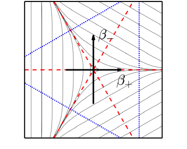
Figure 1: Potential picture for the tumbling case. The black contour lines represent the curvature potential while the dotted (blue) and dashed (red) lines represent the rotation and centrifugal walls, respectively.

II.4.1 Special classes of solutions

Before doing the numerics, we comment on particular classes of solutions: one class of solutions is obtained if we choose, for example, the initial conditions $v_{1}=0=v_{2}$ and $v_{3}=1$. The geodesic equation (34) implies now that the velocities stay constant in time. This implies that at all times $l_{1}=0=l_{2}$ and $l_{3}=p_{\psi}=p_{T}C$. This class of solutions is known as the non-tumbling case. Furthermore, there are classes of solutions which are rotating versions of the Taub solution. These solutions should be divided into two subclasses: one class that oscillates between the centrifugal walls and the curvature potential and one class that runs through the valley straight into the singularity. We set

$$v_{1}=v_{2}=\frac{1}{2}\ ,v_{3}=0\quad\text{and}\quad\beta_{-}=0.$$ (36)

For the $\Gamma_{i}$ variables it means that $\Gamma_{1}=\textnormal{e}^{2\alpha}\textnormal{e}^{2\beta_{+}}=\Gamma_{2}$ and $\Gamma_{3}=\textnormal{e}^{2\alpha}\textnormal{e}^{-4\beta_{+}}$. With this choice we obtain $I_{3}=0$ and $3I_{1}=3I_{2}=\sinh^{2}\left(3\beta_{+}\right)$. Most importantly, the geodesic equation (34) is trivially satisfied, that is, $v_{1}=v_{2}=1/2$ and $v_{3}=0$ for all times. When setting $C=0$ we obtain the diagonal case which contains the isotropic case of a closed Friedmann universe. The simulation plotted in Fig. 2 was performed for the tumbling case, that is, the $v_{i}$ are chosen to be non-zero.

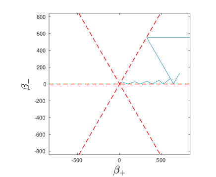
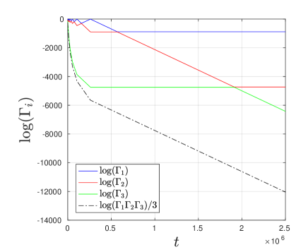
Figure 2: Numerical simulation of the tumbling case. In the region where $0<t<5\times 10^{5}$ (arbitrary units) one can see a typical Kasner era. The solution bounces in the valley formed between the curvature and one of the centrifugal potential walls. Increasing $t$ corresponds to evolution towards the singularity.

II.4.2 The asymptotic regime close to the singularity

In order to simplify the dynamics of the general case, BKL made two assumptions based on qualitative considerations of the equations of motion. The first assumption states that anisotropy of space grows without bound. This means that the solution enters the regime

$$\Gamma_{1}\gg\Gamma_{2}\gg\Gamma_{3}.$$ (37)

The ordering of indices is irrelevant. In fact, there are six possible orderings of indices which each correspond to the universe point being constrained to one of the six regions bounded by the rotation and centrifugal walls sketched in Fig. 1. The region $\Gamma_{1}>\Gamma_{2}>\Gamma_{3}$ corresponds to the right region above the line $\beta_{-}=0$ in Fig. 1. More precisely, the inequality (37) means that

$$\Gamma_{2}/\Gamma_{1}\rightarrow 0\quad\text{and}\quad\Gamma_{3}/\Gamma_{2}\rightarrow 0\ .$$ (38)

Our numerical simulations support the validity of this assumption (see the plot of the ratios $\Gamma_{2}/\Gamma_{1}$ and $\Gamma_{3}/\Gamma_{2}$ in Fig. 3). We provide plots of the two ratios $\Gamma_{2}/\Gamma_{1}$, $\Gamma_{3}/\Gamma_{2}$ and the velocities $\vec{v}$ in order to provide a sanity check of the approximation we will perform later on.

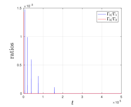
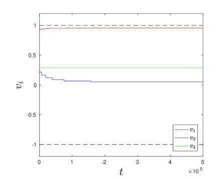
Figure 3: Plots of the ratios $\Gamma_{2}/\Gamma_{1}$, $\Gamma_{3}/\Gamma_{2}$ and the velocity $\vec{v}$. The plots correspond to the numerical solution presented in Fig. 2. The peaks in the ratios appear during bounces of the universe point with the centrifugal walls. As we can see, the height of these peaks decreases in the evolution towards the singularity.

The second assumption made by BKL states that the Euler angles assume constant values:

$$(\theta,\phi,\psi)\rightarrow(\theta_{0},\phi_{0},\psi_{0})\ ,$$ (39)

that is, the rotation of the principal axes stops for all practical purposes and the metric becomes effectively diagonal. The analysis of BKL bkl supports the consistency of making both assumptions at the same time. Similar heuristic considerations can possibly be applied to other Bianchi models as well Jantzen:2001me . In the dust model under consideration, this assumption is equivalent to the statement that the dust velocities $\vec{v}$ assume constant values $\vec{v}\rightarrow\vec{v}^{(0)}$. Our numerical results indicate that this is in fact true (see Fig. 3). BKL then arrive at the simplified effective set of equations.

Let us now carry out the approximation and apply it to our equations of motion. The kinetic term stays untouched during the approximation. The first step in the approximation is to ignore the rotational potential. In view of the strong inequality (37), we approximate the curvature potential via

$$\Gamma_{1}^{2}+\Gamma_{2}^{2}+\Gamma_{3}^{2}-2(\Gamma_{1}\Gamma_{2}+\Gamma_{3}\Gamma_{1}+\Gamma_{2}\Gamma_{3})\approx\Gamma_{1}^{2}\ .$$ (40)

Furthermore, we approximate the centrifugal potential by

$$\frac{l_{1}^{2}}{I_{1}}+\frac{l_{2}^{2}}{I_{2}}+\frac{l_{3}^{2}}{I_{3}}\approx 12C^{2}p_{T}^{2}\left[\frac{\Gamma_{3}}{\Gamma_{2}}\left(v^{(0)}_{1}\right)^{2}+\frac{\Gamma_{2}}{\Gamma_{1}}\left(v^{(0)}_{3}\right)^{2}\right]\ .$$ (41)

Note that one centrifugal wall was ignored completely. Having Fig. 1 in mind, this approximation is well motivated since only two of the centrifugal walls are expected to have a significant influence on the dynamics of the universe point. After defining the new variables

$$a\equiv\Gamma_{1}\ ,\quad b\equiv 2p_{T}^{\prime 2}C^{2}\left(v^{(0)}_{3}\right)^{2}\Gamma_{2},\quad c\equiv 4p_{T}^{\prime 4}C^{4}\left(v^{(0)}_{1}v^{(0)}_{3}\right)^{2}\Gamma_{3},$$ (42)

we arrive at a simplified Hamiltonian constraint and equations of motion,

$$(\log a)^{\cdot}(\log b)^{\cdot}+(\log a)^{\cdot}(\log c)^{\cdot}+(\log b)^{\cdot}(\log c)^{\cdot}=a^{2}+b/a+c/b,$$ (43)

$$(\log a)^{\cdot\cdot}=b/a-a^{2},\quad(\log b)^{\cdot\cdot}=a^{2}-b/a+c/b,\quad(\log c)^{\cdot\cdot}=a^{2}-c/b,$$

which coincides with the asymptotic form of equations obtained in bkl . Equations (43) can now be treated by the numerical methods which we have used in the previous sections. One must ensure that initial conditions are chosen such that the simulation starts close to the asymptotic regime (37).

III Conclusions

The numerical simulations indicate that the non-diagonal Bianchi IX solutions, with tilted dust, evolve into the regime where $\Gamma_{1}\gg\Gamma_{2}\gg\Gamma_{3}$ and $v_{i}\approx$const. The results motivate us to formulate the conjecture:

Given a tumbling solution to the general Bianchi IX model filled with pressureless tilted matter, there exists $t_{0}\in\mathbb{R}$ such that the solution is well approximated by a solution to the asymptotic equations of motion for all times $t>t_{0}$ describing the vicinity of the singularity.

To make the notion of “approximation” mathematically more precise, a suitable measure of the “distance” on the set of solutions is needed. For this purpose, we propose to use the following simple measure:

$$\Delta(t)\equiv\sqrt{\left(\log\Gamma_{1}(t)-\log\bar{a}(t)\right)^{2}+\left(\log\Gamma_{2}(t)-\log\bar{b}(t)\right)^{2}+\left(\log\Gamma_{3}(t)-\log\bar{c}(t)\right)^{2}},$$ (44)

where $\{\Gamma_{1},\Gamma_{2},\Gamma_{3}\}$ denotes the numerical solution to the exact equations of motion (33)–(34), and

$$a=\bar{a}\ ,\quad b=2p_{T}^{\prime 2}C^{2}\left(v^{(0)}_{3}\right)^{2}\bar{b}\ ,\quad c=4p_{T}^{\prime 4}C^{4}\left(v^{(0)}_{1}v^{(0)}_{3}\right)^{2}\bar{c}\$$ (45)

denote the numerical solution to the asymptotic equations of motion (43).

We have evolved the exact system of equations from $t=0$ forward in time until $t=3\times 10^{6}$. There we used the same initial conditions as the ones we used to obtain the solution shown in Fig. 2. We then took the final state at $t=3\times 10^{6}$ as an initial condition for the asymptotic system of equations and evolved it backwards in time towards the re-bounce until $t=-980$.

Fig. 4 presents the measure (44) as a function of time. We can see fast decrease of $\Delta$ with increasing time (evolution towards the singularity) and fast increase of $\Delta$ with decreasing time (evolution away from the singularity).

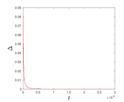
(a)

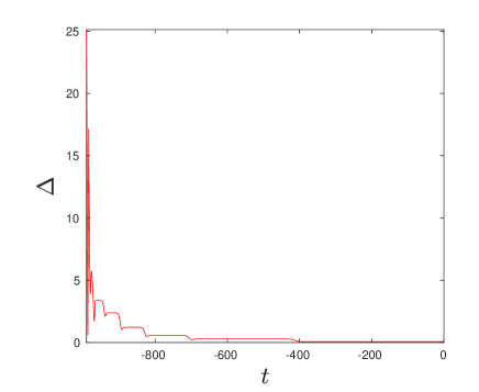
(b)

Figure 4: The difference between the exact and the asymptotic solutions: (a) evolution towards the singularity, (b) evolution away from the singularity.

Our numerical simulations give strong support to the conjecture concerning the asymptotic dynamics of the general Bianchi IX spacetime put forward long ago by Belinski, Khalatnikov, and Ryan bkl . We remark that approximating the diagonal or non-tumbling case by the asymptotic dynamics (43) is invalid (see ENW for more details).

It is sometimes stated that “matter does not matter” in the asymptotic regime, but this does not mean that one is allowed to use the dynamics of the purely diagonal case. One only encounters an effectively diagonal case, which is expressed in terms of the directional scale factors $\{a,b,c\}$. So there exist serious differences between the purely diagonal and effectively diagonal cases (see ENW for more details).

Employing the asymptotic form of the equations of motion may enable one to study the chaotic behaviour and other properties of the solution space for the general model. This is also important for quantizing the general Bianchi IX model, where the quantization of the exact dynamics seems to be quite difficult, whereas the quantization of the asymptotic case seems to be feasible AGWP .

Appendix A Numerical analysis

Numerical simulations of the diagonal Bianchi IX model were already carried out in the late 1980s and early 1990s (see e.g. Berger_1990 ; Hobill_1991 ; for a modern account, see Berger ). Our main interest here is in the nondiagonal case. With given initial conditions (respecting the constraints $\mathcal{H}=0$), the system (33) and (34) can be integrated by using a suitable numerical method. In this work we employ the MATLAB R2016b solver ode113 matlab_ode . This code is an implementation of an Adams-Bashforth-Moulton method. It turns out to lead to the best results when compared to other MATLAB solvers. The relative error tolerance of the solver was chosen to be of the order $10^{-14}$. We can integrate the equations of motion together with the geodesic equation to obtain a numerical solution to the system. We set up initial conditions at $t=0$ and evolve the system forward in time towards the final singularity and away from the rebounce.

A major problem in numerical relativity is that the Hamiltonian constraint is not preserved exactly by the numerical procedure. Similar to Berger_1990 ; Hobill_1991 , we find that the error in the Hamiltonian constraint varies strongest after the start of the simulation. Furthermore, it varies strongly when the evolution of the universe approaches the point of maximal expansion. While approaching the singularity, the error approaches an approximately constant value. This can be seen in Fig. 5. Therefore we can minimize the error when we choose the initial conditions far away from the point of maximal expansion. Moreover, it turned out that the error can be further reduced when constraining the solver’s maximally allowed time step size. This time step size should, however, not be chosen too small since small time step sizes can drive the propagation of round off errors. Small step sizes are, of course, also numerically more expensive. By manually fine tuning the initial conditions and the maximally allowed time step size it was possible to keep the order of the error lower than $10^{-15}$.

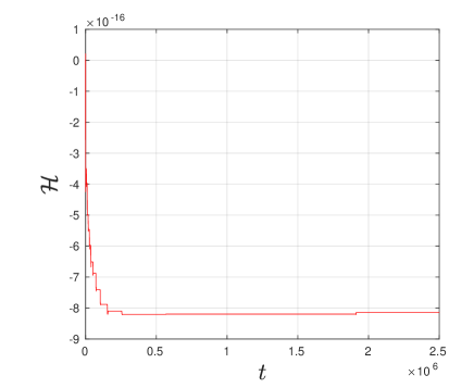
(a)

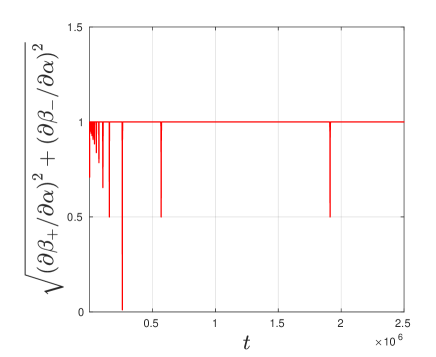
(b)

Figure 5: Subfigure (a) shows the error in the Hamiltonian constraint. Subfigure (b) shows the speed of the universe point in the beta plane as measured in “$\alpha$-time”. This plot can be viewed as another check of the numerics. Between two successive bounces from the potential walls this quantity should be close to one. If this ceased to be true it would indicate that the error in the Hamiltonian constraint becomes relevant and cannot be neglected in the approach towards the singularity (see Berger for a more detailed discussion). Both plots correspond to the numerical solution shown in Fig. 2.

Recall that the dynamics of Bianchi IX are chaotic, that is, slightly changing initial conditions have a large effect on the long time behaviour of solutions. Since the propagation of random numerical errors cannot be avoided, we will be dealing with a “butterfly effect” and it should in general not be expected that our numerical solution is an actual approximation of some exact solution of the equations of motion when considering large time intervals.

References

- (1) S. Hawking and R. Penrose, The Nature of Space and Time (Princeton University Press, Princeton, 1996).
- (2) C. Kiefer, Quantum Gravity, third edition (Oxford University Press, Oxford, 2012).
- (3) I. Albarran, M. Bouhmadi-López, C. Kiefer, J. Marto, and P. V. Moniz, “Classical and quantum cosmology of the little rip abrupt event”, Phys. Rev. D 94, 063536 (2016).
- (4) A. Kamenshchik, C. Kiefer, and N. Kwidzinski, “Classical and quantum cosmology of Born-Infeld type models”, ibid. 93, 083519 (2016).
- (5) H. Bergeron, E. Czuchry, J. P. Gazeau, P. Małkiewicz, and W. Piechocki, “Smooth quantum dynamics of the mixmaster universe,” Phys. Rev. D 92 061302 (2015).
- (6) H. Bergeron, E. Czuchry, J. P. Gazeau, P. Małkiewicz, and W. Piechocki, “Singularity avoidance in a quantum model of the mixmaster universe,” Phys. Rev. D 92, 124018 (2015).
- (7) B. K. Berger, “Singularities in cosmological spacetimes”, in: Springer Handbook of Spacetime, edited by A. Ashtekar and V. Petkov (Springer, Berlin, 2014), pp. 437–460.
- (8) C. Uggla, “Spacetime singularities: recent developments”, Int. J. Mod. Phys. D 22, 1330002 (2013).
- (9) E. Czuchry, D. Garfinkle, J. R. Klauder, and W. Piechocki, “Do spikes persist in a quantum treatment of spacetime singularities?”, Phys. Rev. D 95, 024014 (2017).
- (10) E. Lifshitz, “On the gravitational stability of the expanding universe”, J. Phys. (USSR) 10, 116 (1946). Republished as a Golden Oldie in: Gen. Relativ. Grav. 49, 18 (2017), with an editorial note by G. F. R. Ellis.
- (11) E. M. Lifshitz and I. M. Khalatnikov, “Investigations in Relativistic Cosmology”, Adv. Phys. 12, 185 (1963).
- (12) V. Belinski and M. Henneaux, The Cosmological Singularity (Cambridge University Press, Cambridge, 2017). See also V. A. Belinski, “On the cosmological singularity”, Int. J. Mod. Phys. D 23, 1430016 (2014) for a shorter review.
- (13) V. A. Belinskii, I. M. Khalatnikov, and E. M. Lifshitz, “Oscillatory approach to a singular point in the relativistic cosmology”, Adv. Phys. 19, 525 (1970).
- (14) V. A. Belinskii, I. M. Khalatnikov, and E. M. Lifshitz, “A general solution of the Einstein equations with a time singularity”, Adv. Phys. 31, 639 (1982).
- (15) N. J. Cornish and J. J. Levin, “The Mixmaster universe: A chaotic Farey tale,” Phys. Rev. D 55, 7489 (1997).
- (16) J.M. Heinzle, C. Uggla, and N. Rohr, “The cosmological billiard attractor”, Adv. Theor. Math. Phys. 13, 293 (2009).
- (17) D. Garfinkle, “Numerical simulations of generic singularities”, Phys. Rev. Lett. 93, 161101 (2004).
- (18) C. W. Misner, “Mixmaster universe”, Phys. Rev. Lett. 22, 1071 (1969).
- (19) C. W. Misner, “Quantum cosmology I”, Phys. Rev. 186, 1319 (1969).
- (20) M. P. Ryan, “Qualitative cosmology: diagrammatic solutions for Bianchi type IX universes with expansion, rotation, and shear. I. The symmetric case”, Ann. Phys. (N.Y.) 65, 506 (1971).
- (21) M. P. Ryan, “Qualitative cosmology: diagrammatic solutions for Bianchi type IX universes with expansion, rotation, and shear. II. The general case”, Ann. Phys. (N.Y.) 68, 541 (1971).
- (22) R. T. Jantzen, “Spatially homogeneous dynamics: a unified picture”, arXiv:gr-qc/0102035. Originally published in the Proceedings of the International School Enrico Fermi, Course LXXXVI (1982) on Gamov Cosmology, edited by R. Ruffini and F. Melchiorri (North Holland, Amsterdam, 1987), pp. 61–147.
- (23) L. Andersson and A. D. Rendall, “Quiescent cosmological singularities”, Commun. Math. Phys. 218, 479 (2001).
- (24) J. D. Barrow, “Quiescent cosmology”, Nature 272, 211 (1978).
- (25) A. Góźdź, W. Piechocki, and G. Plewa, “Quantum Belinski-Khalatnikov-Lifshitz scenario”, in preparation.
- (26) O. I. Bogoyavlenskii, “Some properties of the type IX cosmological model with moving matter”, Sov. Phys. JETP 43, 187 (1976).
- (27) M. P. Ryan and L. C. Shepley, Homogeneous Relativistic Cosmologies (Princeton University Press, Princeton, 1975).
- (28) M. P. Ryan, Hamiltonian Cosmology (Springer, Berlin, 1972).
- (29) J. D. Brown and K. V. Kuchar̆, “Dust as a standard of space and time in canonical quantum gravity”, Phys. Rev. D 51, 5600 (1995).
- (30) T. Damour and P. Spindel, “Quantum Einstein-Dirac Bianchi universes”, Phys. Rev. D 83, 123520 (2011).
- (31) V. A. Belinskii, I. M. Khalatnikov, and M. P. Ryan, “The oscillatory regime near the singularity in Bianchi-type IX universes”, Preprint 469 (1971), Landau Institute for Theoretical Physics, Moscow (unpublished); published as sections 1 and 2 in M. P. Ryan, Ann. Phys. (N.Y.) 70, 301 (1971).
- (32) E. Czuchry, N. Kwidzinski, and W. Piechocki, “Comparing the dynamics of diagonal and general BIX spacetimes”, in preparation.
- (33) B. K. Berger, “Numerical study of initially expanding mixmaster universes”, Class. Quant. Grav. 7, 203 (1990).
- (34) D. Hobill, D. Bernstein, M. Welge, and D. Simkins, “The Mixmaster cosmology as a dynamical system”, Class. Quant. Grav. 8, 1155 (1991).
- (35) L. F. Shampine and M. W. Reichelt, “The MATLAB ODE Suite”, SIAM Journal on Scientific Computing 18, 1 (1997).