A $c/\mu$-Rule for Service Resource Allocation in Group-Server Queues

Abstract

This paper addresses a dynamic on/off server scheduling problem in a queueing system with Poisson arrivals and $K$ groups of exponential servers. Servers within each group are homogeneous and between groups are heterogeneous. A scheduling policy prescribes the number of working servers in each group at every state $n$ (number of customers in the system). Our goal is to find the optimal policy to minimize the long-run average cost, which consists of an increasing convex holding cost for customers and a linear operating cost for working servers. We prove that the optimal policy has monotone structures and quasi bang-bang control forms. Specifically, we find that the optimal policy is indexed by the value of $c-\mu G(n)$, where $c$ is the operating cost rate, $\mu$ is the service rate, and $G(n)$ is called perturbation realization factor. Under a reasonable condition of scale economies, we prove that the optimal policy obeys a so-called $c$/$\mu$-rule. That is, the servers with smaller $c$/$\mu$ should be turned on with higher priority. With the monotone property of $G(n)$, we further prove that the optimal policy has a multi-threshold structure when the $c$/$\mu$-rule is applied. Numerical experiments demonstrate that the $c/\mu$-rule has a good scalability and robustness.

Keywords: Group-server queue, dynamic scheduling, $c/{\mu}$-rule, resource allocation

1 Introduction

Queueing models are often formulated to study stochastic congestion problems in manufacturing and service systems, computer and communication networks, social economics, etc. Research on queueing models is spreading from performance evaluation to performance optimization for system design and control. Queueing phenomena is caused by limited service resource. How to efficiently allocate the service resource is a fundamental issue in queueing systems, which continually attracts attention from the operational research community, such as several papers published in Oper. Res. in recent volumes [12, 45].

In practice, there exists a category of queueing systems with multiple servers that provide homogeneous service at different service rates and costs. These servers can be categorized into different groups. Servers in the same group have the same service rate and cost rate, while those in different groups are heterogeneous in these two rates. Customers wait in line when all the servers are busy. Running a server (keeping a server on) will incur operating cost and holding a customer will incur waiting cost. There exists a tradeoff between these costs. Keeping more servers on will increase the operating cost but decrease the holding cost. The holding cost is increasingly convex in queue length and the operating cost is linear in the number of working servers. The system controller can dynamically turn on or off servers according to different backlogs (queue lengths) such that the system long-run average cost can be minimized. We call such queueing models group-server queues [30]. Note that any queueing system with heterogeneous servers can be considered as a group-server queue if the servers with the same service cost and rate are grouped as a class. Following are some examples that motivate the group-server queueing model.

• Multi-tier storage systems: As illustrated in Fig. 1(a), such a multi-tier storage architecture is widely used in intelligent storage systems, where different storages are structured as multiple tiers and data are stored and migrated according to their hotness (access frequency) [50, 63]. Solid state drive (SSD), hard disk drive (HDD), and cloud storage are organized in a descending order of their speeds and costs. A group-server queue fits such a system and can be used to study the system performance, such as the response time of I/O requests. It is an interesting topic to find the optimal architecture and scheduling of I/O requests so that the desired system throughput is achieved at a minimum cost.

• Clustered computing systems: As illustrated in Fig. 1(b), the computing facilities of a server farm are organized in clusters. Computers in different clusters have different performance and power consumption. For example, high performance computer (HPC) has greater processing rate and more power consumption. Computing jobs can be scheduled and migrated among computers. Energy efficiency is one of the key metrics for evaluating the performance of data centers. Power management policy aims to dynamically schedule servers’ working states (e.g., high/low power, or sleep) according to workloads such that power consumption and processing rate can be traded-off in an optimal way [15, 25].

• Human staffed service systems: One example is a call center that might have several groups of operators (customer representatives) in different locations (or different countries). Depending on the demand level, the number of operator groups attending calls may be dynamically adjusted. The service efficiencies and operating costs of these groups can be different although operators in each group can be homogeneous in these two aspects. Another example is the operation of a food delivery company, such as GrubHub in the US or Ele.me in China, which has several restaurant partners with good reputation. During the high demand period, the limited number of its own delivery drivers (servers in group 1) may not be able to deliver food orders to customers in a promised short time (due to long queues). Thus, the company can share part of their delivery service demands with another less reputable food delivery company who also owns a set of drivers (servers in group 2).

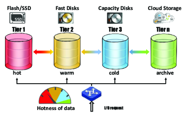
(a) A multi-tier storage system.

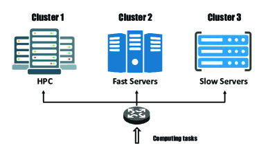
(b) A clustered computing system.

Figure 1: Motivations of group-server queues.

Similar resource allocation problems may exist in other systems such as clustered wireless sensor networks [28], tiered web site systems [46], tiered tolling systems [24], etc. The common features of these problems can be well captured by the group-server queue. How to efficiently schedule the server groups to optimize the targeted performance metrics is an important issue for both practitioners and queueing researchers. To address this issue, we focus on finding the optimal on/off server scheduling policy in a group-server queue to minimize the long-run average cost.

1.1 Related Research

Service resource allocation problems in queueing systems are widely studied in the literature. One stream of research focuses on the service rate control which aims to find the optimal service rates such that the system average cost (holding cost plus operating cost) can be minimized. This type of problems are mainly motivated by improving the operational efficiency of computer and telecommunication systems. For a server with a fixed service rate, turning it on or off can be considered as a service rate control of full or zero service rate. The optimality of threshold type policy, such as $N$-policy, $D$-policy, and $T$-policy, has been studied in single-server queueing systems with fixed service rate [4, 20, 21]. Then, further studies extend single-server systems to multi-server networks, such as cyclic queues or tandem queues [38, 43, 53], where the optimality of bang-bang control or threshold type policy is studied. Note that the bang-bang control means that even for the case where the service rate can be chosen in a finite range, the optimal rate is always at either zero or the maximum rate depending on the system size (threshold). For complicated queueing networks, such as Jackson networks, it has been proved that the bang-bang control is optimal when the cost function has a linear form to service rates, using the techniques of linear programming by Yao and Schechner [60] and derivative approach by Ma and Cao [33], respectively. Recent works by Xia et al. further extend such optimality structure from a linear cost function to a concave one [56, 57]. Another line of studying the service rate control problem is from a game theoretic viewpoint [18, 55]. We cannot enumerate all service rate control studies due to space limit of this paper. A common feature of the past studies is to characterize the structure of optimal rate control policy in a variety of queueing systems.

The tradeoff between holding cost and operating cost is also a major issue in some service systems with human servers. Thus, there exist many studies on server scheduling problems (or called staffing problems) which aim to dynamically adjust the number of servers to minimize the average holding and operating costs. An early work is by Yadin and Naor who study the dynamic on/off scheduling policy of a server in an $M/G/1$ queue with a non-zero setup time [59]. Many other related works can be found in this area and we just name a few [7, 13, 42, 61]. To control the customer waiting time and improve the server utilization, Zhang studies a congestion-based staffing (CBS) policy for a multi-server service system motivated by the US-Canada border-crossing stations [62]. Servers in these studies are assumed to be homogeneous. The CBS policy has a two-threshold structure and can be considered as a generalization of the multi-server queue with server vacations, which is an important class of queueing models [44].

Job assignment problem in heterogenous servers is closely related to the on/off server scheduling problem treated in this paper. It has one queue and multiple servers. It focuses on optimal scheduling of homogeneous jobs at heterogeneous servers with different service rates and/or operating costs. In one class of problems, the objective is to minimize the average waiting time of jobs under the assumption that only holding cost is relevant and the operating cost is sunk (i.e., not considered). In addition, when a job is assigned to a server, it cannot be reassigned to other faster (more desirable) server which becomes available later. Such a problem is also called a slow-server problem and can be used to study the job routing policy in computer systems. One pioneering work is by Lin and Kumar and they study the optimal control of an M/M/2 queue with two heterogeneous servers. They prove that the faster server should be always utilized while the slower one should be utilized only when the queue length exceeds a computable threshold value [31, 49]. For the case with more than two servers, it is shown that the fastest available server (FAS) rule is optimal [35]. However, for other servers except for FAS, it is difficult to directly extend the single threshold (two-server system) to the multi-threshold optimality (more than two-server system), although it looks intuitive. This is because the system state becomes higher dimensional that makes the dynamic programming based analysis very complicated. Weber proposes a conjecture about the threshold optimality for multiple heterogenous servers and shows that the threshold may depend on the state of slower servers [52]. Rykov proves this conjecture using dynamic programming [39] and Luh and Viniotis prove it using linear programming [32], but their proofs are opaque or incomplete [11]. Armony and Ward further study a fair dynamic routing problem, in which the customer average waiting time is minimized at the constraint of a fair idleness portion of servers [2, 51]. Constrained Markov decision processes and linear programming models are utilized to characterize that the optimal routing policy asymptotically has a threshold type in a limit regime with many servers [2]. There are numerous studies on the slow-server problem from various perspectives, which are summarized in [1, 19, 58].

When job reassignment (also called job migration) is allowed, the slow-server problem becomes trivial since it is optimal to always assign jobs to available fastest servers. However, when the server operating cost (such as power consumption) is considered, the job assignment problem is not trivial even with job migration allowed. In fact, both holding and operating costs should be considered in practical systems, such as energy efficient data centers or cloud computing facilities [14]. Akgun et al. give a comprehensive study on this problem [1]. They utilize the duality between the individually optimal and socially optimal policies [17, 58] to prove the threshold optimality of heterogenous servers for a clearing system (no arrivals) with or without reassignment. They also prove the threshold optimality for the less preferred server in a two-server system with customer arrivals. It is shown that the preference of servers depends on not only their service rates, but also the usage costs (operating costs), holding costs, arrival rate, and the system state.

Under a cost structure with both holding and operating costs, the job assignment problem for heterogeneous servers with customer arrivals and job migration can be viewed as an equivalence to our on/off server scheduling problem in a group-server queue. In this paper, we characterize the structure of the optimal policy which can significantly simplify the computation of the parameters of the optimal on/off server schedule. In general, under the optimal policy, a server group will not be turned on only if the ratio of operating cost rate $c$ to service processing rate $\mu$ is smaller than a computable quantity $G(n)$, called perturbation realization factor. The perturbation realization factor depends on the number of customers in the system (system state), the arrival rate, and the cost function. We call this type of policy an index policy and it has a form of state-dependent multi-threshold. The term of state-dependent means that the preference rankings of groups (the order of server groups to be turned on) will change from one state to another. However, under a reasonable condition of server group’s scale economies, the optimal index policy is reduced to a state-independent multi-threshold policy, called the $c/\mu$-rule. This simple rule is easy to implement in practice and complements the well-known $c\mu$-rule for polling queues. In a polling queueing system, a single server serves multiple classes of customers which form multiple queues and a polling policy prescribes which queue to serve by the single server. In a group-server queueing system, heterogeneous servers grouped into multiple classes serve homogeneous customers (a single queue) and an on/off server schedule prescribes which server group is turned on to serve the single queue. Note that the “$c$” in the $c\mu$-rule is the customer waiting cost rate, while the “$c$” in the $c/\mu$-rule is the server operating cost rate. Due to the difference in the cost rate $c$, it is intuitive that the customer class with the highest $c\mu$ value should be served first and the server group with the lowest $c/\mu$ value should be utilized first. Although these results are kind of intuitive, the $c\mu$-rule was studied long time ago but the $c/\mu$-rule was not well established until this paper. This may be because of the more complexity caused by the heterogeneous server system. Note that although the $c/\mu$ rankings order the server’s operating cost per unit of service rate, different service rates impact the customer holding cost differently. In contrast, in a polling queueing system, the only cost difference between polling two different queues is the $c\mu$, the holding cost moving out of the system per unit of time. Thus, a static $c\mu$-rule can be established as an optimal policy to minimize the system average cost.

The early work of the $c\mu$-rule can be traced back to Smith’s paper in 1956 under a deterministic and static setting [41]. Under the $c\mu$-rule, the queue with larger $c\mu$ value should be served with higher priority. This rule is very simple and easy to implement in practice. It stimulates numerous extensions in the literature [23, 26, 27, 36, 48]. Many works aim to study similar properties to the $c\mu$-rule under various queueing systems and assumptions. For example, Baras et al. study the optimality of the $c\mu$-rule from 2 to $K$ queues with linear costs and geometric service requirement [5, 6], and Buyukkoc et al. revisit the proof of the $c\mu$-rule in a simple way [8]. Van Mieghem studies the asymptotic optimality of a generalized version of the $c\mu$-rule with convex holding costs in heavy traffic settings [47]. This work is then extended by Mandelbaum and Stolyar to a network topology [34]. Atar et al. further study another generalized version called the $c\mu/\theta$ rule in an abandonment queue where $\theta$ is the abandonment rate of impatient customers [3]. Recently, Saghafian and Veatch study the $c\mu$-rule in a two-tiered queue [40]. In contrast to the extensive studies on the $c\mu$-rule in the literature, there are few studies on the $c/\mu$ rule for the resource allocation in a single queue with heterogeneous servers.

1.2 Our Contributions

One of the significant differences between our work and relevant studies in the literature is that the servers in our model are heterogeneous and categorized into multiple groups, which makes the model more general but more complex. Most heterogenous server models in the literature may be viewed as a special case of our model, in which each group has only one server. Thus, our model is more applicable to large scale service systems such as data centers. Moreover, we assume that there is an unlimited waiting room for customers, which means that the dynamic policy is over an infinite state space. To find the optimal policy over the infinite state space is difficult. Thus, we aim to characterize the structure of the optimal policy. While the holding cost in job assignment problems is usually assumed to be linear, we assume the holding cost can be any increasing convex function (a generalization of linear function). We formulate this service resource allocation problem in a group-server queue as a Markov decision process (MDP). Unlike the traditional MDP approach, we utilize the sensitivity-based optimization theory to characterize the structure of the optimal policy and develop efficient algorithms to compute the optimal policy and thresholds.

The main contribution of this paper can be summarized in the following aspects.

• Index policy: The server preference (priority of being turned on) is determined by an index $c-\mu G(n)$, where $G(n)$ is the perturbation realization factor and it is computable and state-dependent. Servers with more negative value of $c-\mu G(n)$ have more preference to be turned on. Servers with positive $c-\mu G(n)$ should be kept off. The value of $G(n)$ will affect the preference order of servers and depends on $n$, arrival rate, and cost functions. We prove the optimality of this index policy and show that $G(n)$ plays a fundamental role in determining the optimal index policy.

• The $c/\mu$-rule: Under the condition of scale economies for server groups, the preference of servers can be determined by their $c/\mu$ values, instead of $c-\mu G(n)$. Thus, the preference order of servers is independent of $n$, arrival rate, and cost functions. The server’s on/off scheduling policy becomes the $c/\mu$ rule. Under this rule, the server with smaller $c/\mu$ should be turned on with higher priority. Searching the optimal policy over an infinite-dimensional mapping space is reduced to searching the optimal multiple thresholds. Multi-threshold policy is easier to be implemented in practice and robust.

• Optimality structures: With the performance difference formula, we derive a necessary and sufficient condition of the optimal policy. The optimality of quasi bang-bang control is also established. The monotone and convexity properties of performance potentials and perturbation realization factors, which are fundamental quantities during optimization, are established. With these properties, the optimality of index policy and the $c/\mu$ rule is proved. The structure of optimal policy is characterized well and the optimization complexity is reduced significantly.

Besides the theoretical contributions in the above aspects, using the performance difference formula, we decompose the original problem into an infinite number of integer linear programs. Based on the structure of the optimal policy, we develop iterative algorithms to find the optimal index policy or optimal multi-threshold policy. Here, the $c/\mu$-rule can be utilized to simplify the search algorithms significantly. These algorithms are similar to the policy iteration in the traditional MDP theory and their performance is demonstrated by numerical examples.

1.3 Paper Organization

The rest of the paper is organized as follows. In Section 2, a model of group-server queue is developed to capture the heterogeneity of servers. An optimization problem is formulated to determine the on/off server scheduling policy of cost minimization. The analysis is presented in Section 3, where the structure of optimal index policy is characterized based on the perturbation realization factor of server groups. In Section 4, we derive the $c/\mu$-rule and study the optimality of multi-threshold policy under the condition of scale economies. In Section 5, we conduct numerical experiments to gain the managerial insights and to show the efficiency of our approach. Finally, the paper is concluded in Section 6 with a summary.

2 Optimization Problem in Group-Server Queues

In this section, we describe the service resource allocation problem in a group-server queue model. This model can be used to represent a waiting line with heterogeneous servers classified into a finite number of groups, which can also be called parallel-server systems in previous studies [2]. Servers are homogeneous within the group and are heterogeneous between groups. A group-server queue is shown in Fig. 2 and described as follows.

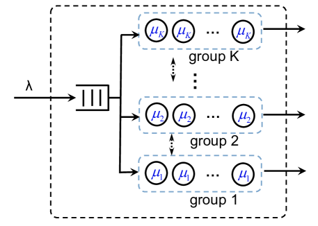
Figure 2: An example of group-server queue model, where servers are in parallel.

Customers arrive to a service station with multiple groups of servers according to a Poisson process with rate $\lambda$. The waiting room is infinite and the service discipline is first-come-first-serve (FCFS). The service times of each server are assumed to be independent and exponentially distributed. The heterogeneous servers are classified into $K$ groups. Each group has $M_{k}$ servers, which can be turned on or off, $k=1,2,\cdots,K$. When a server in group $k$ is turned on, it will work at service rate $\mu_{k}$ and consume an operating cost $c_{k}$ per unit of time. Servers in the same group are homogeneous, i.e., they have the same service rate $\mu_{k}$ and cost rate $c_{k}$, $k=1,2,\cdots,K$. Servers in different groups are heterogeneous in $\mu_{k}$ and $c_{k}$. We assume that servers in different groups offer the same service, i.e., customers are homogeneous. In general, services offered by different groups may be different and the connection of groups may be cascaded, or even interconnected. Such a setting can be called a group-server queueing network. When a working server has to be turned off, the customer being served at that server is interrupted and transferred to the waiting room or another idle server if available. Due to the memoryless property of the service time, such an interruption has no effect on customer’s remaining service time.

The system state $n$ is defined as the number of customers in the system (including those in service). The on/off status of servers need not be included in the system state because free customer migrations among servers are allowed in the model. Thus, the state space is the nonnegative integer set $\mathbb{N}$, which is infinite. At each state $n\in\mathbb{N}$, we determine the number of working servers in each group, which can be represented by a $K$-dimensional row vector as

$$\bm{m}:=(m_{1},m_{2},\cdots,m_{K}),$$ (1)

where $m_{k}$ is the number of working servers in group $k$, i.e., $m_{k}\in\mathbb{Z}_{[0,M_{k}]}$, $k=1,2,\cdots,K$. We call $\bm{m}$ the scheduling action at state $n$, according to the terminology of MDPs. Thus, the action space is defined as

$$\mathbb{M}:=\mathbb{Z}_{[0,M_{1}]}\times\mathbb{Z}_{[0,M_{2}]}\times\cdots\times\mathbb{Z}_{[0,M_{K}]},$$ (2)

where $\times$ is the Cartesian product. We assume that the system has reached a steady state under a condition to be specified later in Proposition 2. Therefore, a stationary scheduling policy $d$ is defined as a mapping from the infinite state space $\mathbb{N}$ to the finite action space $\mathbb{M}$, i.e., $d:\mathbb{N}\rightarrow\mathbb{M}$. If $d$ is determined, we will adopt action $d(n)$ at every state $n$ and $d(n,k)$ is the number of working servers of group $k$, where $n\in\mathbb{N}$ and $k=1,2,\cdots,K$. All possible $d$’s form the policy space $\mathcal{D}$, which is an infinite dimensional searching space.

When the system state is $n$ and the scheduling action $\bm{m}=d(n)$ is adopted, a holding cost $h(n)$ and an operating cost $o(\bm{m})$ will be incurred per unit of time. In the literature, it is commonly assumed that the operating cost is increasing with respect to (w.r.t.) the number of working servers. In this paper, we define the linear operating cost function $o(\bm{m})$ as follows.

$$o(\bm{m}):=\sum_{k=1}^{K}m_{k}c_{k}=\bm{m}\bm{c},$$ (3)

where $\bm{c}:=(c_{1},c_{2},\cdots,c_{K})^{T}$ is a $K$-dimensional column vector and $c_{k}$ represents the operating cost rate per server in group $k$. Therefore, the total cost rate function of the whole system per time unit is defined as

$$f(n,\bm{m}):=h(n)+\bm{m}\bm{c}.$$ (4)

We make the following assumption regarding the customer’s holding cost (waiting cost) and the server’s setup cost (changeover cost).

Assumption 1.

$h(n)$ is an increasing convex function w.r.t. $n$ and $h(n)\rightarrow\infty$ when $n\rightarrow\infty$. The server’s setup cost is negligible.

Such a holding cost assumption is widely used in the literature [47] and represents the situation where the delay cost grows rapidly as the system becomes more congested. For a non-empty state $n$, if a scheduling action $\bm{m}$ is adopted, some working servers may be turned off and services of customers at those servers will be interrupted. These customers will be returned to the waiting room or reassigned to other currently available working servers. Such a rule is called non-resume transfer discipline. Since the setup cost for turning on a server (including transferring a customer to an available server) is zero, we do not have to keep track of the number of on (or off) servers for any state. Otherwise, each server’s status must be included in the definition of the system state so that the state space will be changed from one dimensional to multi-dimensional one, which is much more complex.

Denote by $n_{t}$ the number of customers in the system at time $t\geq 0$. The long-run average cost of the group-server queue under policy $d$ can be written as

$$\eta^{d}:=\lim\limits_{T\rightarrow\infty}\mathbb{E}\left\{\frac{1}{T}\int_{0}^{T}f(n_{t},d(n_{t}))\mathrm{d}t\right\}.$$ (5)

The objective is to find the optimal policy $d^{*}$ such that the associated long-run average cost is minimized. That is,

$$d^{*}=\operatorname*{argmin}\limits_{d\in\mathcal{D}}\{\eta^{d}\}.$$ (6)

Remark 1. It is worth noting that the scheduling policy $d$ is a mapping from an infinite state space to a $K$-dimensional finite action space. The state space is infinite and the action space grows exponentially with $K$. Thus, the policy space $\mathcal{D}$ to be searched is of infinite dimension. Characterizing the optimal structure of such a mapping is challenging but necessary in solving this optimization problem. A major contribution of this paper is to accomplish this challenging task and derive a simple $c/\mu$-rule as the optimal policy under a certain condition.

3 Optimal Policy Structure

The optimization problem (6) can be modeled as a continuous-time MDP with the long-run average cost criterion. The traditional theory of MDPs is based on the well-known Bellman optimality equation. However, in a multi-server queueing model with infinite buffer, it may be difficult to characterize the structure of the optimal policy using the traditional approach. Recently, Cao proposed the sensitivity-based optimization (SBO) theory [10]. This relatively new theory provides a new perspective to optimize the performance of Markov systems. The key idea of the SBO theory is to utilize the performance sensitivity information, such as the performance difference or the performance derivative, to conduct the optimization of stochastic systems. It may even treat the stochastic optimization problems to which the dynamic programming fails to offer the solution [10, 56, 57]. We use the SBO theory to characterize the structure of the optimal policy of the optimization problem (6).

First, we study the structure of the action space. Owing to zero setup cost, we should turn off any idle servers and obtain the following result immediately.

Proposition 1.

The optimal action $\bm{m}$ at state $n$ satisfies $\bm{m}\bm{1}\leq n$, where $\bm{1}$ is a column vector with proper dimension and its all elements are 1’s.

Note that if the server setup cost is not zero, this proposition may not hold. From Proposition 1, for every state $n$, we can define the efficient action space $\mathbb{M}_{n}$ as

$$\mathbb{M}_{n}:=\{\mbox{all }\bm{m}\in\mathbb{M}:\bm{m}\bm{1}\leq n\}.$$ (7)

A policy $d$ is said to be efficient if $d(n)\in\mathbb{M}_{n}$ for every $n\in\mathbb{N}$. Accordingly, the efficient policy space $\mathcal{D}_{e}$ is defined as

$$\mathcal{D}_{e}:=\{\mbox{all }d:d(n)\in\mathbb{M}_{n},\forall n\in\mathbb{N}\}.$$ (8)

Therefore, in the rest of the paper, we limit our optimal policy search in $\mathcal{D}_{e}$. For any efficient action $\bm{m}\in\mathbb{M}_{n}$, the total service rate of the queueing system is $\bm{m}\bm{\mu}$, where $\bm{\mu}$ is a $K$-dimensional column vector of service rates defined as

$$\bm{\mu}:=(\mu_{1},\mu_{2},\cdots,\mu_{K})^{T}.$$ (9)

For the continuous-time MDP formulated in (6), we define the performance potential as follows [10].

$$g(n):=\mathbb{E}\left\{\int_{0}^{\infty}[f(n_{t},d(n_{t}))-\eta]\mathrm{d}t\Big{|}n_{0}=n\right\},\quad n\in\mathbb{N},$$ (10)

where $\eta$ is defined in (5) and we omit the superscript ‘$d$’ for simplicity. The definition (10) indicates that $g(n)$ quantifies the long-run accumulated effect of the initial state $n$ on the average performance $\eta$. In the traditional MDP theory, $g(n)$ can also be understood as the relative value function or bias [37].

By using the strong Markov property, we can decompose the right-hand-side of (10) into two parts as follows.

$$g(n) = \mathbb{E}\{\tau\}[f(n,d(n))-\eta]+\mathbb{E}\left\{\int_{\tau}^{\infty}[f(n_{t},d(n_{t}))-\eta]\mathrm{d}t\Big{|}n_{0}=n\right\}$$ (11)

$$= \frac{1}{\lambda+d(n)\bm{\mu}}[f(n,d(n))-\eta]+\frac{\lambda}{\lambda+d(n)\bm{\mu}}\mathbb{E}\left\{\int_{\tau}^{\infty}[f(n_{t},d(n_{t}))-\eta]\mathrm{d}t\Big{|}n_{\tau}=n+1\right\}$$

$$+\frac{d(n)\bm{\mu}}{\lambda+d(n)\bm{\mu}}\mathbb{E}\left\{\int_{\tau}^{\infty}[f(n_{t},d(n_{t}))-\eta]\mathrm{d}t\Big{|}n_{\tau}=n-1\right\},$$

where $\tau$ is the sojourn time at the current state $n$ and $\mathbb{E}\{\tau\}=\frac{1}{\lambda+d(n)\bm{\mu}}$.

Combining (10) and (11), we have the recursion

$$\begin{array}[]{ll}\left[\lambda+d(n)\bm{\mu}\right]g(n)=f(n,d(n))-\eta+\lambda g(n+1)+d(n)\bm{\mu}g(n-1),&\quad n\geq 1;\\ \lambda g(n)=f(n,d(n))-\eta+\lambda g(n+1),&\quad n=0.\\ \end{array}$$ (12)

We denote $\bm{B}$ as the infinitesimal generator of the Markov process under an efficient policy $d\in\mathcal{D}_{e}$. Due to nature of the continuous-time Markov process, the elements of $\bm{B}$ are: for a state $n\geq 1$, $B(n,n)=-\lambda-d(n)\bm{\mu}$, $B(n,n+1)=\lambda$, $B(n,n-1)=d(n)\bm{\mu}$, $B(n,:)=0$ otherwise. Therefore, with such a birth-death process, $\bm{B}$ can be written as the following form

$$\bm{B}=\left[\begin{array}[]{cccccc}-\lambda&\lambda&0&0&0&\cdots\\ d(1)\bm{\mu}&-\lambda-d(1)\bm{\mu}&\lambda&0&0&\cdots\\ 0&d(2)\bm{\mu}&-\lambda-d(2)\bm{\mu}&\lambda&0&\cdots\\ 0&0&d(3)\bm{\mu}&-\lambda-d(3)\bm{\mu}&\lambda&\cdots\\ \vdots&\vdots&\vdots&\ddots&\ddots&\ddots\\ \end{array}\right].$$ (13)

Hence, we can rewrite (12) as follows.

$$\begin{array}[]{ll}-B(n,n)g(n)=f(n,d(n))-\eta+B(n,n+1)g(n+1)+B(n,n-1)g(n-1),&n\geq 1;\\ -B(n,n)g(n)=f(n,d(n))-\eta+B(n,n+1)g(n+1),&n=0.\\ \end{array}$$ (14)

We further denote $\bm{g}$ and $\bm{f}$ as the column vectors whose elements are $g(n)$’s and $f(n,d(n))$’s, respectively. We can rewrite (14) in a matrix form as below.

$$\bm{f}-\eta\bm{1}+\bm{B}\bm{g}=\bm{0}.$$ (15)

The above equation is also called the Poisson equation for continuous-time MDPs with long-run average criterion [10]. As $\bm{g}$ is called performance potential or relative value function, we can set $g(0)=\zeta$ and recursively solve $g(n)$ based on (14), where $\zeta$ is any real number. Using matrix operations, we can also evaluate $\bm{g}$ by solving the infinite dimensional Poisson equation (15) through numerical computation techniques, such as RG-factorizations [29].

For the stability of the queueing system, we impose a sufficient condition as follows.

Proposition 2.

If there exists a constant $\tilde{n}$ and for any $n\geq\tilde{n}$, we always have $d(n)\bm{\mu}>\lambda$, then this group-server queue under policy $d$ is stable and its steady state distribution $\bm{\pi}$ exists.

Proposition 2 ensures that $\bm{\pi}$ exists under a proper selection of policy $d$. Thus, we have

$$\begin{array}[]{l}\bm{\pi}\bm{B}=\bm{0},\\ \bm{\pi}\bm{1}=1.\\ \end{array}$$ (16)

The long-run average cost of the system can be written as

$$\eta=\bm{\pi}\bm{f}.$$ (17)

Suppose the scheduling policy is changed from $d$ to $d^{\prime}$, where $d,d^{\prime}\in\mathcal{D}_{e}$. Accordingly, all the associated quantities under the new policy $d^{\prime}$ will be denoted by $\bm{B}^{\prime}$, $\bm{f}^{\prime}$, $\bm{\pi}^{\prime}$, $\eta^{\prime}$, etc. Obviously, we have $\bm{\pi}^{\prime}\bm{B}^{\prime}=\bm{0}$, $\bm{\pi}^{\prime}\bm{1}=1$, and $\eta^{\prime}=\bm{\pi}^{\prime}\bm{f}^{\prime}$.

Left-multiplying $\bm{\pi}^{\prime}$ on both sides of (15), we have

$$\bm{\pi}^{\prime}\bm{f}-\eta\bm{\pi}^{\prime}\bm{1}+\bm{\pi}^{\prime}\bm{B}\bm{g}=0.$$ (18)

Using $\bm{\pi}^{\prime}\bm{B}^{\prime}=\bm{0}$, $\bm{\pi}^{\prime}\bm{1}=1$, and $\eta^{\prime}=\bm{\pi}^{\prime}\bm{f}^{\prime}$ , we can write (18) as

$$\eta^{\prime}-\bm{\pi}^{\prime}\bm{f}^{\prime}+\bm{\pi}^{\prime}\bm{f}-\eta+\bm{\pi}^{\prime}\bm{B}\bm{g}-\bm{\pi}^{\prime}\bm{B}^{\prime}\bm{g}=0,$$ (19)

which gives the performance difference formula for the continuous-time MDP as follows [10].

$$\eta^{\prime}-\eta=\bm{\pi}^{\prime}[(\bm{B}^{\prime}-\bm{B})\bm{g}+(\bm{f}^{\prime}-\bm{f})].$$ (20)

Equation (20) provides the sensitivity information about the system performance, which can be used to achieve the optimization. It clearly quantifies the performance change due to a policy change. Although the exact value of $\bm{\pi}^{\prime}$ may not be known for every new policy $d^{\prime}$, all its entries are always nonnegative and even positive for those positive recurrent states. Therefore, if we choose a proper new policy (with associated $\bm{B}^{\prime}$ and $\bm{f}^{\prime}$) such that the elements of the column vector represented by the square bracket in (20) are always nonpositive, then we have $\eta^{\prime}-\eta\leq 0$ and the long-run average cost of the system will be reduced. If there is at least one negative element in the square bracket for a positive recurrent state, then we have $\eta^{\prime}-\eta<0$ and the system average cost will be reduced strictly. This is the main idea for policy improvement based on the performance difference formula (20).

Using (20), we examine the sensitivity of scheduling policy on the long-run average cost of the group-server queue. Suppose that we choose a new policy $d^{\prime}$ which is the same as the current policy $d$ except for the action at a particular state $n$. For this state $n$, policy $d$ selects action $\bm{m}$ and policy $d^{\prime}$ selects action $\bm{m}^{\prime}$, where $\bm{m},\bm{m}^{\prime}\in\mathbb{M}_{n}$. Substituting (4) and (13) into (20), we have

$$\eta^{\prime}-\eta = \bm{\pi}^{\prime}[(\bm{B}^{\prime}-\bm{B})\bm{g}+(\bm{f}^{\prime}-\bm{f})]$$ (21)

$$= \pi^{\prime}(n)[(\bm{B}^{\prime}(n,:)-\bm{B}(n,:))\bm{g}+(f^{\prime}(n)-f(n))]$$

$$= \pi^{\prime}(n)\left[\sum_{k=1}^{K}(m^{\prime}_{k}-m_{k})\mu_{k}(g(n-1)-g(n))+(\bm{m}^{\prime}\bm{c}-\bm{m}\bm{c})\right]$$

$$= \pi^{\prime}(n)\sum_{k=1}^{K}(m^{\prime}_{k}-m_{k})\left[c_{k}-\mu_{k}(g(n)-g(n-1))\right],$$

where $g(n)$ is the performance potential of the system under the current policy $d$. The value of $g(n)$ can be numerically computed based on (15) or online estimated based on (10). Details can be found in Chapter 3 of [10].

For the purpose of analysis, we define a new quantity $G(n)$ as below.

$$G(n):=g(n)-g(n-1),\quad n=1,2,\cdots.$$ (22)

Note that $G(n)$ quantifies the performance potential difference between neighboring states $n$ and $n-1$. According to the theory of perturbation analysis (PA) [9, 22], $G(n)$ is called perturbation realization factor (PRF) which measures the effect on the average performance when the initial state is perturbed from $n-1$ to $n$. For our specific problem (6), in certain sense, $G(n)$ can be considered as the benefit of reducing the long-run average holding cost due to operating a server. In the following analysis, $G(n)$ plays a fundamental role of directly determining the optimal scheduling policy for the group-server queue.

Based on the recursive relation of $\bm{g}$ in (12), we can also develop the following recursions for computing $G(n)$’s.

Lemma 1.

The PRF $G(n)$ can be computed by the following recursive relations

$$\begin{array}[]{l}G(n+1)=\frac{d(n)\bm{\mu}}{\lambda}G(n)+\frac{\eta-f(n,d(n))}{\lambda},\quad n\geq 1,\\ G(1)=\frac{\eta-f(0,d(0))}{\lambda}.\\ \end{array}$$ (23)

Proof.

From the second equation in (12), we have

$$G(1)=g(1)-g(0)=\frac{\eta-f(0,d(0))}{\lambda}.$$ (24)

Using the first equation in (12), we have

$$\lambda(g(n+1)-g(n))=d(n)\bm{\mu}(g(n)-g(n-1))+\eta-f(n,d(n)),\quad n\geq 1.$$ (25)

Substituting (22) into the above equation, we directly have

$$G(n+1)=\frac{d(n)\bm{\mu}}{\lambda}G(n)+\frac{\eta-f(n,d(n))}{\lambda},\quad n\geq 1.$$ (26)

Thus, the recursions for $G(n)$ are proved. ∎

Substituting (22) into (21), we obtain the following performance difference formula in terms of $G(n)$ when the scheduling action at a single state $n$ is changed from $\bm{m}$ to $\bm{m}^{\prime}$.

$$\eta^{\prime}-\eta=\pi^{\prime}(n)\sum_{k=1}^{K}(m^{\prime}_{k}-m_{k})\left(c_{k}-\mu_{k}G(n)\right).$$ (27)

This difference formula can be extended to a general case when $d$ is changed to $d^{\prime}$, i.e. $d(n)$ is changed to $d^{\prime}(n)$ for all $n\in\mathbb{N}$. Substituting the associated $(\bm{B},\bm{f})$ and $(\bm{B}^{\prime},\bm{f}^{\prime})$ into (20) yields

$$\eta^{\prime}-\eta=\sum_{n\in\mathbb{N}}\pi^{\prime}(n)\sum_{k=1}^{K}(d^{\prime}(n,k)-d(n,k))\left(c_{k}-\mu_{k}G(n)\right).$$ (28)

Based on (28), we can directly obtain a condition for generating an improved policy as follows.

Theorem 1.

If a new policy $d^{\prime}\in\mathcal{D}_{e}$ satisfies

$$(d^{\prime}(n,k)-d(n,k))\left({c_{k}}-{\mu_{k}}G(n)\right)\leq 0$$ (29)

for all $k=1,2,\cdots,K$ and $n\in\mathbb{N}$, then $\eta^{\prime}\leq\eta$. Furthermore, if for at least one state-group pair $(n,k)$, the inequality in (29) strictly holds, then $\eta^{\prime}<\eta$.

Proof.

Since (29) holds for every $n$ and $k$ and $\pi^{\prime}(n)$ is always positive for ergodic processes, it follows from (28) that $\eta^{\prime}-\eta\leq 0$. Thus, the first part of the theorem is proved. The second part can be proved using a similar argument. ∎

Theorem 1 provides a way to generate improved policies based on the current feasible policy. For the system under the current policy $d$, we compute or estimate $G(n)$’s based on its definition. For every state $n$ and server group $k$, if we find $\frac{c_{k}}{\mu_{k}}>G(n)$, then we choose a smaller $d^{\prime}(n,k)$; if we find $\frac{c_{k}}{\mu_{k}}<G(n)$, then we choose a larger $d^{\prime}(n,k)$ satisfying the condition $d^{\prime}(n)\bm{1}\leq n$, as stated by Proposition 1. Therefore, according to Theorem 1, the new policy $d^{\prime}$ obtained from this procedure will perform better than the current policy $d$. This procedure can be repeated to continually reduce the system average cost.

Note that the condition above is only a sufficient one to generate improved policies. Now, we establish a necessary and sufficient condition for the optimal scheduling policy as follows.

Theorem 2.

A policy $d^{*}$ is optimal if and only if its element $d^{*}(n)$, i.e., $(d^{*}(n,1),\cdots,d^{*}(n,K))$, is the solution to the following integer linear programs

$$\mbox{\emph{ILP Problem:}}\hskip 28.45274pt\left\{\begin{array}[]{l}\min\limits_{d(n,k)}\left\{\sum_{k=1}^{K}d(n,k)(c_{k}-\mu_{k}G^{*}(n))\right\}\\ \mbox{s.t.}\quad 0\leq d(n,k)\leq M_{k},\\ \hskip 28.45274pt\sum_{k=1}^{K}d(n,k)\leq n,\end{array}\right.$$ (30)

for every state $n\in\mathbb{N}$, where $G^{*}(n)$ is the PRF defined in (22) under policy $d^{*}$.

Proof.

First, we prove the sufficient condition. Suppose $d^{*}(n)$ is the solution to the ILP problem (30), $\forall n\in\mathbb{N}$. For any other policy $d^{\prime}\in\mathcal{D}_{e}$, we know that it must satisfy the constraints in (30) and

$$\sum_{k=1}^{K}d^{\prime}(n,k)(c_{k}-\mu_{k}G^{*}(n))\geq\sum_{k=1}^{K}d^{*}(n,k)(c_{k}-\mu_{k}G^{*}(n)),\quad\forall n\in\mathbb{N},$$ (31)

since $d^{*}(n)$ is the solution to (30). Substituting (31) into (28), we obtain

$$\eta^{\prime}-\eta^{*}=\sum_{n\in\mathbb{N}}\pi^{\prime}(n)\sum_{k=1}^{K}(d^{\prime}(n,k)-d^{*}(n,k))(c_{k}-\mu_{k}G^{*}(n))\geq 0,$$ (32)

for any $d^{\prime}\in\mathcal{D}_{e}$. Therefore, $\eta^{*}$ is the minimal average cost of the scheduling problem (6) and $d^{*}$ is the optimal policy. The sufficient condition is proved.

Second, we use contradiction to prove the necessary condition. Assume that the optimal policy $d^{*}$ is not always the solution to the ILP problem (30). That is, at least for a particular state $n$, there exists another $d(n)$ which is the solution to (30) and satisfies

$$\sum_{k=1}^{K}d(n,k)(c_{k}-\mu_{k}G^{*}(n))<\sum_{k=1}^{K}d^{*}(n,k)(c_{k}-\mu_{k}G^{*}(n)).$$ (33)

Therefore, we can construct a new policy $d^{\prime}$ as follows: It chooses the action $d(n)$ at the state $n$ only and chooses the same actions prescribed by $d^{*}$ at other states. Substituting $d^{\prime}$ and $d^{*}$ into (28) gives

$$\eta^{\prime}-\eta^{*}=\pi^{\prime}(n)\sum_{k=1}^{K}(d(n,k)-d^{*}(n,k))(c_{k}-\mu_{k}G^{*}(n)).$$ (34)

Substituting (33) into the above equation and using the fact $\pi^{\prime}(n)>0$ for any positive recurrent state $n$, we have $\eta^{\prime}<\eta^{*}$, which contradicts the assumption that $d^{*}$ is the optimal policy. Thus, the assumption does not hold and $d^{*}$ should be the solution to (30). The necessary condition is proved. ∎

Theorem 2 indicates that the original scheduling problem (6) can be converted into a series of ILP problem (30) at every state $n\in\mathbb{N}$. However, it is impossible to directly solve an infinite number of ILP problems since the state space is infinite. To get around this difficulty, we further investigate the structure of the solution to these ILPs.

By analyzing (30), we can find that the solution to the ILP problem must have the following structure:

• For those groups with $c_{k}-\mu_{k}G^{*}(n)>0$, we have $d^{*}(n,k)=0$;

• For those groups with $c_{k}-\mu_{k}G^{*}(n)<0$, we repeat letting $d^{*}(n,k)=M_{k}$ or as large as possible in an ascending order of $c_{k}-\mu_{k}G^{*}(n)$, under the constraint $\sum_{k=1}^{K}d(n,k)\leq n$.

Then, we can further specify the above necessary and sufficient condition of the optimal policy as follows.

Theorem 3.

A policy $d^{*}$ is optimal if and only if its element $d^{*}(n)$ satisfies the condition: If $G^{*}(n)>\frac{c_{k}}{\mu_{k}}$, then $d^{*}(n,k)=M_{k}\wedge(n-\sum_{l=1}^{k-1}d^{*}(n,l))$; otherwise, $d^{*}(n,k)=0$, for $k=1,2,\cdots,K$, where the index of server groups should be renumbered in an ascending order of $c_{k}-\mu_{k}G^{*}(n)$ at the current state $n$, $n\in\mathbb{N}$.

With Theorem 3, we can see that the optimal policy can be fully determined by the value of $c_{k}-\mu_{k}G^{*}(n)$. Such a policy form is called an index policy and $c_{k}-\mu_{k}G^{*}(n)$ can be viewed as an index, which has similarity to the Gittins’ index or Whittle’s index for solving multi-armed bandit problems [16, 54].

Theorem 3 also reveals the quasi bang-bang control structure of the optimal policy $d^{*}$. That is, the optimal number of working servers in group $k$ is either 0 or $M_{k}$, except for the group that first violates the efficient condition in Proposition 1. For any state $n$, after the group index is renumbered according to Theorem 3, the optimal action always has the following form

$$d^{*}(n)=(M_{1},M_{2},\cdots,M_{\hat{k}-1},M_{\hat{k}}\wedge(n-\sum_{l=1}^{\hat{k}-1}M_{l}),0,0,\cdots,0),$$ (35)

where $\hat{k}$ is the first group index that violates the constraint $\sum_{l=1}^{\hat{k}}M_{l}\leq n$ or $c_{\hat{k}+1}-\mu_{\hat{k}+1}G^{*}(n)<0$, i.e.,

$$\hat{k}:=\min\left\{k:\sum_{l=1}^{k}M_{l}>n,\mbox{ or }\frac{c_{k+1}}{\mu_{k+1}}\geq G^{*}(n)\right\}.$$ (36)

Therefore, $\hat{k}$ can also be viewed as a threshold and we have $\hat{k}\in\{0,1,\cdots,K\}$. Such a policy can be called a quasi threshold policy with threshold $\hat{k}$. Under this policy, the number of servers to be turned on for each group is as follows.

$$\left\{\begin{array}[]{ll}d^{*}(n,l)=M_{l},&\mbox{if }l<\hat{k};\\ d^{*}(n,l)=0,&\mbox{if }l>\hat{k};\\ d^{*}(n,l)=M_{\hat{k}}\wedge(n-\sum_{l=1}^{\hat{k}-1}M_{l}),&\mbox{if }l=\hat{k}.\\ \end{array}\right.$$ (37)

If threshold $\hat{k}$ is determined, $d^{*}(n)$ is also determined. Thus, finding $d^{*}(n)$ becomes finding the threshold $\hat{k}$, which simplifies the search for the optimal policy. However, we note that the index order of groups is renumbered according to the ascending value of $c_{k}-\mu_{k}G^{*}(n)$, which is varied at different state $n$ or different value of $G^{*}(n)$. On the other hand, the value of $\hat{k}$ also depends on the system state $n$, $n\in\mathbb{N}$. Therefore, the index order of groups and the threshold $\hat{k}$ will both vary at different state $n$, which makes the quasi threshold policy not easy to implement in practice. To further characterize the optimal policy, we explore its other structural properties.

Difference formula (28) and Theorem 3 indicate that $c_{k}-\mu_{k}G(n)$ is an important quantity to differentiate the server groups. If $c_{k}-\mu_{k}G(n)<0$, turning on servers in group $k$ can reduce the system average cost. Group $k$ can be called an economic group for the current system. Therefore, we define $\mathbb{K}_{n}$ as the economic group set at the current state $n$

$$\mathbb{K}_{n}:=\left\{k:G(n)>\frac{c_{k}}{\mu_{k}}\right\}.$$ (38)

We should turn on severs in the economic groups $\mathbb{K}_{n}$ as many as possible, subject to $d(n)\bm{1}\leq n$. Note that $G(n)$ reflects the reduction of the holding cost due to operating a server, from a long-run average perspective.

With Theorems 2 and 3, the optimization problem (6) for each state $n$ can be solved by finding the solution to each subproblem in (30) with the structure of quasi bang-bang control or quasi threshold form like (35). However, since the number of ILPs is infinite, we need to establish the monotone property of PRF $G(n)$ which can convert the infinite state space search to a finite state space search for the optimal policy. To achieve this goal, we first establish the convexity of performance potential $g^{*}(n)$.

Theorem 4.

The performance potential $g^{*}(n)$ under the optimal policy $d^{*}$ is increasing and convex in $n$.

Proof.

We prove this theorem by induction. Since the problem (6) is a continuous time MDP with the long-run average cost criterion, the optimal policy $d^{*}$ should satisfy the Bellman optimality equation as follows.

$$\min\limits_{\bm{m}\in\mathbb{M}_{n}}\left\{f(n,\bm{m})-\eta^{*}+\bm{B}(n,:|\bm{m})\bm{g}^{*}\right\}=0,\quad\forall n\in\mathbb{N},$$ (39)

where $\bm{B}(n,:|\bm{m})$ is the $n$th row of the infinitesimal generator $\bm{B}$ defined in (13) if action $\bm{m}$ is adopted.

Define $\Lambda$ as any constant that is larger than the maximal absolute value of all elements in $\bm{B}$ under any possible policy. Without loss of generality, we further define

$$\Lambda:=\sup\limits_{n,\bm{m}}\{|B(n,n|\bm{m})|\}=\lambda+\sum_{k=1}^{K}M_{k}\mu_{k}.$$ (40)

Then we can use the Bellman optimality equation to derive the recursion for value iteration as follows.

$$\Lambda g_{l+1}(n) = \min\limits_{\bm{m}\in\mathbb{M}_{n}}\left\{f(n,\bm{m})-\eta_{l}+\sum_{n^{\prime}\in\mathbb{N}}B(n,n^{\prime}|\bm{m})g_{l}(n^{\prime})+\Lambda g_{l}(n)\right\}$$ (41)

$$= \min\limits_{\bm{m}\in\mathbb{M}_{n}}\left\{h(n)+\bm{m}\bm{c}-\eta_{l}+(\Lambda-\lambda-\bm{m}\bm{\mu})g_{l}(n)+\lambda g_{l}(n+1)+\bm{m}\bm{\mu}g_{l}(n-1)\right\},$$

where the second equality holds because of using (4) and (14), $g_{l}(n)$ is the performance potential (relative value function) of state $n$ at the $l$th iteration, and $\eta_{l}$ is the long-run average cost at the $l$th iteration. By defining

$$A(n):=h(n)+\bm{m}\bm{c}-\eta_{l}+(\Lambda-\lambda-\bm{m}\bm{\mu})g_{l}(n)+\lambda g_{l}(n+1)+\bm{m}\bm{\mu}g_{l}(n-1),$$ (42)

we can rewrite (41) as

$$\Lambda g_{l+1}(n)=\min\limits_{\bm{m}\in\mathbb{M}_{n}}\left\{A(n)\right\}.$$ (43)

It is well known from the MDP theory [37] that the initial value of $g_{0}$ can be any value. Therefore, we set $g_{0}(n)=0$ for all $n$, which satisfies the increasing and convex property. Now we use the induction to establish this property. Suppose $g_{l}(n)$ is increasing and convex in $n$. We need to show that $g_{l+1}(n)$ also has this property. If done, we know that $g_{l}(n)$ is increasing and convex in $n$ for all $l$. In addition, since the value iteration converges to the optimal value function, i.e.,

$$\lim\limits_{l\rightarrow\infty}g_{l}(n)=g^{*}(n),\quad n\in\mathbb{N},$$ (44)

Then, we can conclude that $g^{*}(n)$ is increasing and convex in $n$. The induction is completed in two steps.

First step, we prove the increasing property of $g_{l+1}(n)$ or $g_{l+1}(n+1)-g_{l+1}(n)\geq 0$. Using (43), we have

$$\Lambda[g_{l+1}(n+1)-g_{l+1}(n)]=\min\limits_{\bm{m}\in\mathbb{M}_{n+1}}\{A(n+1)\}-\min\limits_{\bm{m}\in\mathbb{M}_{n}}\left\{A(n)\right\}.$$ (45)

Denote $\bm{m}^{*}_{n+1}$ as the optimal action in $\mathbb{M}_{n+1}$, which achieves the minimum for $A(n+1)$ in (43). Below, we want to use $\bm{m}^{*}_{n+1}$ to remove the operators $\min\limits_{\bm{m}\in\mathbb{M}_{n}}\{\cdot\}$ in (45), which has to be discussed in two cases by concerning whether $\bm{m}^{*}_{n+1}\in\mathbb{M}_{n}$.

Case ①: $\bm{m}^{*}_{n+1}\in\mathbb{M}_{n}$, we can directly use $\bm{m}^{*}_{n+1}$ to replace $\min\limits_{\bm{m}\in\mathbb{M}_{n}}\{\cdot\}$ in (45) and obtain

$$\Lambda[g_{l+1}(n+1)-g_{l+1}(n)] \geq A(n+1)|_{\bm{m}^{*}_{n+1}}-A(n)|_{\bm{m}^{*}_{n+1}}$$ (46)

$$=h(n+1)+\bm{m}^{*}_{n+1}\bm{c}-\eta_{l}+(\Lambda-\lambda-\bm{m}^{*}_{n+1}\bm{\mu})g_{l}(n+1)+\lambda g_{l}(n+2)+\bm{m}^{*}_{n+1}\bm{\mu}g_{l}(n)$$

$$-[h(n)+\bm{m}^{*}_{n+1}\bm{c}-\eta_{l}+(\Lambda-\lambda-\bm{m}^{*}_{n+1}\bm{\mu})g_{l}(n)+\lambda g_{l}(n+1)+\bm{m}^{*}_{n+1}\bm{\mu}g_{l}(n-1)]$$

$$=[h(n+1)-h(n)]+(\Lambda-\lambda-\bm{m}^{*}_{n+1}\bm{\mu})[g_{l}(n+1)-g_{l}(n)]$$

$$+\lambda[g_{l}(n+2)-g_{l}(n+1)]+\bm{m}^{*}_{n+1}\bm{\mu}[g_{l}(n)-g_{l}(n-1)].$$

From Assumption 1 that $h(n)$ is increasing in $n$, the first term of RHS of (46) is non-negative. Moreover, we already assume that $g_{l}(n)$ is increasing in $n$. We also know that $(\Lambda-\lambda-\bm{m}^{*}_{n+1}\bm{\mu})\geq 0$ from the definition (40). Therefore, with (46), we have $g_{l+1}(n+1)-g_{l+1}(n)\geq 0$ in this case.

Case ②: $\bm{m}^{*}_{n+1}\notin\mathbb{M}_{n}$, it means that $\bm{m}^{*}_{n+1}\bm{1}=n+1>n$ violating the condition in Proposition 1. In this case, we select an action $\bm{\alpha}$ as below.

$$\bm{\alpha}=\bm{m}^{*}_{n+1}-\bm{e}_{1},\quad\bm{\alpha}\in\mathbb{M}_{n},$$ (47)

where $\bm{e}_{1}$ is a zero vector except one proper element is 1 such that every element of $\bm{\alpha}$ is nonnegative. We use $\bm{\alpha}$ to replace $\min\limits_{\bm{m}\in\mathbb{M}_{n}}\{\cdot\}$ in (45) and obtain

$$\Lambda[g_{l+1}(n+1)-g_{l+1}(n)] \geq A(n+1)|_{\bm{m}^{*}_{n+1}}-A(n)|_{\bm{\alpha}}$$ (48)

$$=h(n+1)+\bm{m}^{*}_{n+1}\bm{c}-\eta_{l}+(\Lambda-\lambda-\bm{m}^{*}_{n+1}\bm{\mu})g_{l}(n+1)+\lambda g_{l}(n+2)+\bm{m}^{*}_{n+1}\bm{\mu}g_{l}(n)$$

$$-[h(n)+\bm{\alpha}\bm{c}-\eta_{l}+(\Lambda-\lambda-\bm{\alpha}\bm{\mu})g_{l}(n)+\lambda g_{l}(n+1)+\bm{\alpha}\bm{\mu}g_{l}(n-1)]$$

$$=[h(n+1)-h(n)]+\bm{e}_{1}\bm{c}+\lambda[g_{l}(n+2)-g_{l}(n+1)]+(\Lambda-\lambda-\bm{m}^{*}_{n+1}\bm{\mu})g_{l}(n+1)$$

$$+\bm{m}^{*}_{n+1}\bm{\mu}g_{l}(n)-[(\Lambda-\lambda-\bm{\alpha}\bm{\mu})g_{l}(n)+\bm{\alpha}\bm{\mu}g_{l}(n-1)].$$

Since $g_{l}(n)$ is increasing in $n$, we have

$$(\Lambda-\lambda-\bm{m}^{*}_{n+1}\bm{\mu})g_{l}(n+1)+\bm{m}^{*}_{n+1}\bm{\mu}g_{l}(n)\geq(\Lambda-\lambda)g_{l}(n);$$ (49)

$$-[(\Lambda-\lambda-\bm{\alpha}\bm{\mu})g_{l}(n)+\bm{\alpha}\bm{\mu}g_{l}(n-1)]\geq-(\Lambda-\lambda)g_{l}(n).$$ (50)

Substituting the above equations into (48), we have

$$\Lambda[g_{l+1}(n+1)-g_{l+1}(n)]\geq[h(n+1)-h(n)]+\bm{e}_{1}\bm{c}+\lambda[g_{l}(n+2)-g_{l}(n+1)]>0.$$ (51)

Combining cases ①&②, we always have $g_{l+1}(n+1)-g_{l+1}(n)\geq 0$ and the increasing property of $g_{l+1}(n)$ is proved.

Second step, we prove the convex property of $g_{l+1}(n)$ or $g_{l+1}(n+1)-2g_{l+1}(n)+g_{l+1}(n-1)\geq 0$. We denote $\bm{m}^{*}_{n-1}$ as the optimal action in $\mathbb{M}_{n-1}$, which achieves the minimum for $A(n-1)$ in (43). From (43), we have

$$\Lambda[g_{l+1}(n+1)-2g_{l+1}(n)+g_{l+1}(n-1)] = \min\limits_{\bm{m}\in\mathbb{M}_{n+1}}\{A(n+1)\}-2\min\limits_{\bm{m}\in\mathbb{M}_{n}}\left\{A(n)\right\}+\min\limits_{\bm{m}\in\mathbb{M}_{n-1}}\{A(n-1)\}$$ (52)

$$= A(n+1)|_{\bm{m}^{*}_{n+1}}-2\min\limits_{\bm{m}\in\mathbb{M}_{n}}\left\{A(n)\right\}+A(n-1)|_{\bm{m}^{*}_{n-1}}.$$

Similarly, we select actions to replace the operators $\min\limits_{\bm{m}\in\mathbb{M}_{n}}\{\cdot\}$ in (52). The actions are generated from $\bm{m}^{*}_{n+1}$ and $\bm{m}^{*}_{n-1}$ and they should belong to the feasible set $\mathbb{M}_{n}$. We select two actions $\bm{\alpha}_{1}$ and $\bm{\alpha}_{2}$ that satisfy

$$\bm{\alpha}_{1}+\bm{\alpha}_{2}=\bm{m}^{*}_{n+1}+\bm{m}^{*}_{n-1},\quad\bm{\alpha}_{1},\bm{\alpha}_{2}\in\mathbb{M}_{n}.$$ (53)

For example, when $n$ is large enough and the condition in Proposition 1 is always satisfied, we can simply select $\bm{\alpha}_{1}=\bm{m}^{*}_{n+1}$ and $\bm{\alpha}_{2}=\bm{m}^{*}_{n-1}$. For other cases where the condition in Proposition 1 may be violated, we can properly adjust the number of working servers based on $\bm{m}^{*}_{n+1}$ and $\bm{m}^{*}_{n-1}$ and always find feasible $\bm{\alpha}_{1}$ and $\bm{\alpha}_{2}$. It is easy to verify and we omit the details for simplicity. Therefore, we use $\bm{\alpha}_{1}$ and $\bm{\alpha}_{2}$ to replace the operators $\min\limits_{\bm{m}\in\mathbb{M}_{n}}\{\cdot\}$ of the two $A(n)$’s in (52) and obtain

$$\Lambda[g_{l+1}(n+1)-2g_{l+1}(n)+g_{l+1}(n-1)]\geq A(n+1)|_{\bm{m}^{*}_{n+1}}-A(n)|_{\bm{\alpha}_{1}}-A(n)|_{\bm{\alpha}_{2}}+A(n-1)|_{\bm{m}^{*}_{n-1}}.$$ (54)

Substituting (42) into the above equation, we have

$$\Lambda[g_{l+1}(n+1)-2g_{l+1}(n)+g_{l+1}(n-1)] \geq [h(n+1)-2h(n)+h(n-1)]+[\bm{m}^{*}_{n+1}\bm{c}-(\bm{\alpha}_{1}+\bm{\alpha}_{2})\bm{c}$$ (55)

$$+\bm{m}^{*}_{n-1}\bm{c}]+(\Lambda-\lambda-\bm{m}^{*}_{n+1}\bm{\mu})g_{l}(n+1)-(2\Lambda-2\lambda-\bm{\alpha}_{1}\bm{\mu}-\bm{\alpha}_{2}\bm{\mu})g_{l}(n)+(\Lambda-\lambda-\bm{m}^{*}_{n-1}\bm{\mu})g_{l}(n-1)$$

$$+\lambda[g_{l}(n+2)-2g_{l}(n)+g_{l}(n-1)]+\bm{m}^{*}_{n+1}\bm{\mu}g_{l}(n)-(\bm{\alpha}_{1}\bm{\mu}+\bm{\alpha}_{2}\bm{\mu})g_{l}(n-1)+\bm{m}^{*}_{n-1}\bm{\mu}g_{l}(n-2).$$

Since $h(n)$ is convex in $n$ (Assumption 1), we have $h(n+1)-2h(n)+h(n-1)\geq 0$. Moreover, it is assumed that $g_{l}(n)$ is convex in $n$, hence $g_{l}(n+2)-2g_{l}(n)+g_{l}(n-1)\geq 0$ holds. By further utilizing (53), we can derive

$$\bm{m}^{*}_{n+1}\bm{c}-(\bm{\alpha}_{1}+\bm{\alpha}_{2})\bm{c}+\bm{m}^{*}_{n-1}\bm{c}=0,$$

$$(\Lambda-\lambda-\bm{m}^{*}_{n+1}\bm{\mu})g_{l}(n+1)-(2\Lambda-2\lambda-\bm{\alpha}_{1}\bm{\mu}-\bm{\alpha}_{2}\bm{\mu})g_{l}(n)+(\Lambda-\lambda-\bm{m}^{*}_{n-1}\bm{\mu})g_{l}(n-1)\geq 0,$$

$$\bm{m}^{*}_{n+1}\bm{\mu}g_{l}(n)-(\bm{\alpha}_{1}\bm{\mu}+\bm{\alpha}_{2}\bm{\mu})g_{l}(n-1)+\bm{m}^{*}_{n-1}\bm{\mu}g_{l}(n-2)\geq 0.$$

Therefore, we know $g_{l+1}(n+1)-2g_{l+1}(n)+g_{l+1}(n-1)\geq 0$ and the convex property of $g_{l+1}(n)$ is proved.

In summary, we have proved that $g_{l}(n)$ is increasing and convex in $n$ by induction, $\forall l\in\mathbb{N}$. Therefore, $g^{*}(n)$ is also increasing and convex in $n$ by (44). This completes the proof. ∎

Since $G(n)=g(n)-g(n-1)$, from Theorem 4, we can directly derive the following theorem about the monotone property of $G^{*}(n)$.

Theorem 5.

The PRF $G^{*}(n)$ under the optimal policy $d^{*}$ is nonnegative and increasing in $n$.

Note that $G(n)$ plays a fundamental role in (27) and (28). Thus, the increasing property of $G^{*}(n)$ enables us to establish the monotone structure of optimal policy $d^{*}$ as follows.

Theorem 6.

The optimal total number of working servers is increasing in $n$. In other words, we have $||d^{*}(n+1)||_{1}\geq||d^{*}(n)||_{1}$, $\forall n\in\mathbb{N}$.

Proof.

Similar to (38), we define $\mathbb{K}^{*}_{n}$ as the set of economic groups under the optimal policy $d^{*}$

$$\mathbb{K}^{*}_{n}:=\left\{k:G^{*}(n)>\frac{c_{k}}{\mu_{k}}\right\}.$$ (56)

Note that $G^{*}(n+1)\geq G^{*}(n)$ from Theorem 5 implies that any $k\in\mathbb{K}^{*}_{n}$ also belongs to $\mathbb{K}^{*}_{n+1}$ or

$$\mathbb{K}^{*}_{n}\subseteq\mathbb{K}^{*}_{n+1}.$$ (57)

Theorem 3 indicates that the optimal total number of working servers equals

$$||d^{*}(n)||_{1}=\sum_{k\in\mathbb{K}^{*}_{n}}d^{*}(n,k)=\left\{\begin{array}[]{ll}\sum_{k\in\mathbb{K}^{*}_{n}}M_{k},&\mbox{ if }n\geq\sum_{k\in\mathbb{K}^{*}_{n}}M_{k};\\ n,&\mbox{ if }n<\sum_{k\in\mathbb{K}^{*}_{n}}M_{k};\\ \end{array}\right.$$ (58)

which means

$$||d^{*}(n)||_{1}=n\wedge\sum_{k\in\mathbb{K}^{*}_{n}}M_{k}.$$ (59)

Therefore, for state $n+1$, we have

$$||d^{*}(n+1)||_{1}=(n+1)\wedge\sum_{k\in\mathbb{K}^{*}_{n+1}}M_{k}.$$ (60)

Utilizing (57) and comparing (59) and (60), we directly obtain

$$||d^{*}(n+1)||_{1}\geq||d^{*}(n)||_{1}.$$ (61)

This completes the proof. ∎

Theorem 6 rigorously confirms an intuitive result that when the queue length increases, more servers should be turned on to alleviate the system congestion, which is also the essence of the congestion-based staffing policy [62]. However, it does not mean that the number of working servers in a particular group is necessarily monotone increasing in $n$ (an example is shown in Fig. 6(b) in Section 5). More detailed discussion will be given by Theorem 8 in the next section. Based on Theorem 6, we can further obtain the following result.

Corollary 1.

For a state $\bar{n}$, if $d^{*}(\bar{n},k)=M_{k}$, $\forall k$, then $d^{*}(n,k)=M_{k}$, $\forall k$ and $n\geq\bar{n}$.

Remark 2. Corollary 1 again confirms an intuitive result that once the optimal action is turning on all servers at certain state $\bar{n}$, then the same action is optimal for all states larger than $\bar{n}$. Therefore, the search for the optimal policy can be limited to the states $n<\bar{n}$ and the infinite state space is truncated without loss of optimality. The difficulty of searching over the infinite state space for the optimal policy can be avoided.

There exists a finite $\bar{n}$ (queue length) for which all servers in all groups must be turned on. Such an existence of $\bar{n}$ can be guaranteed by the linear operating cost and the increasing convex holding cost function (Assumption 1), which can be verified by a simple reasoning. Assume for any given scheduling policy, there is no existence of such an $\bar{n}$, which means that there is at least one idle server no matter how long the queue is (for all states). With the increasing convex holding cost function, when the queue length is long enough, the holding cost reduction due to the work completion by turning on the idle server must exceed the constant increase of server’s operating cost. Then, turning on the idle server at this state must reduce the system average cost. Therefore, the assumed policy is never optimal. The suggested policy of turning on the idle server must occur, which means the existence of $\bar{n}$.

Based on Theorems 1 and 3, we can design a procedure to find the optimal scheduling policy. First, compute the value of $G(n)$ from Lemma 1 and determine the set $\mathbb{K}_{n}$ defined in (38). If $n\geq\sum_{k\in\mathbb{K}_{n}}M_{k}$, turn on all the servers in groups belonging to $\mathbb{K}_{n}$. If $n<\sum_{k\in\mathbb{K}_{n}}M_{k}$, renumber the group indexes and set $d(n,k)=M_{k}\wedge(n-\sum_{l=1}^{k-1}d(n,l))$, as stated in Theorem 3. All the other servers should be off. This process is repeated for $n=1,2,\cdots$, until the state $\bar{n}$ satisfying the condition in Corollary 1 is reached. Set $d(n,k)=M_{k}$ for all $k$ and $n\geq\bar{n}$ so that the whole policy $d$ is determined. Then, we iterate the above procedure under this new policy $d$. New improved policies will be repeatedly generated until the policy cannot be improved and the procedure stops. Based on this procedure, we develop the following Algorithm 1 to find the optimal scheduling policy.

Algorithm 1 An iterative algorithm to find the optimal scheduling policy

1:choose a proper initial policy $d^{*}$, e.g., $d^{*}(n,k)=M_{k}$, $\forall n,k$, which indicates to turn on all servers;

2:repeat

3:     set $d=d^{*}$, $d^{*}=\bm{0}$, and $n=0$;

4:     compute or estimate $\eta$ of the system under policy $d$;

5:     repeat

6:         set $n=n+1$;

7:         compute $G(n)$ by using (23) recursively or by solving (15) and (22);

8:         compute $\mathbb{K}_{n}$ using (38);

9:         if $n\geq\sum_{k\in\mathbb{K}_{n}}M_{k}$ then

10:              set $d^{*}(n,k)=M_{k}$, $\forall k\in\mathbb{K}_{n}$;

11:         else

12:              set $d^{*}(n,k)=M_{k}\wedge(n-\sum_{l=1}^{k-1}d^{*}(n,l))$, where $k\in\mathbb{K}_{n}$ and group indexes $k$’s are renumbered according to ascending order of $c_{k}-\mu_{k}G(n)$, as stated in Theorem 3;

13:         end if

14:     until $d^{*}(n,k)=M_{k},\forall k$

15:     set $\bar{n}=n$;

16:     set $d^{*}(n,k)=M_{k}$, $\forall n\geq\bar{n},\forall k$;

17:until $d=d^{*}$ return optimal $d^{*}$.

From Algorithm 1, we can see that this algorithm can iteratively generate better policies. Such a manner is similar to the policy iteration widely used in the traditional MDP theory. Note that the index order of groups should be renumbered at every state $n$, as stated in line 12 of Algorithm 1. Since the server groups are ranked by the index based on $c_{k}-\mu_{k}G^{*}(n)$, the index sequence varies with state $n$. Moreover, although the total number of working servers $||d^{*}(n)||_{1}$ is increasing in $n$, $d^{*}(n,k)$ is not necessarily monotone increasing in $n$ for a particular group $k$. This means that it is possible that for some $n$ and $k$, we have $d^{*}(n,k)>d^{*}(n+1,k)$, as shown in Fig. 6(b) in Section 5. These complications may make it difficult to implement the optimal scheduling policy in practical service systems with human servers, as the servers have to be turned on or off without a regular pattern. However, as we will discuss in the next section, the group index sequence can remain unchanged if the ratio of cost rate to service rate satisfies a reasonable condition. Then, we can develop a simpler optimal scheduling policy obeying the $c/\mu$-rule, which is much easier to implement in practice.

4 The $c/{\mu}$-Rule

We further study the optimal scheduling policy for the group-server queue when the scale economies in terms of $c/{\mu}$ ratios exist.

Assumption 2.

(Scale Economies) If the server groups are sorted in the order of $\frac{c_{1}}{\mu_{1}}\leq\frac{c_{2}}{\mu_{2}}\leq\cdots\leq\frac{c_{K}}{\mu_{K}}$, then their service rates satisfy $\mu_{1}\geq\mu_{2}\geq\cdots\geq\mu_{K}$.

This assumption is reasonable in some practical situations as it means that a faster server has a smaller operating cost rate per unit of service rate. This can be explained by the effect of the scale economies. For example, in a data center, a faster computer usually has a lower cost per unit of computing capacity. With Assumption 2, we can verify that the group index according to the ascending order of $c_{k}-\mu_{k}G^{*}(n)$ remains unvaried, no matter what the value of $G^{*}(n)$ is. The ascending order of $c_{k}-\mu_{k}G^{*}(n)$ is always the same as the ascending order of $c_{k}/\mu_{k}$. That is, the optimal policy structure in Theorem 3 can be characterized as follows.

Theorem 7.

With Assumption 2, a policy $d^{*}$ is optimal if and only if it satisfies the condition: If $G^{*}(n)>\frac{c_{k}}{\mu_{k}}$, then $d^{*}(n,k)=M_{k}\wedge(n-\sum_{l=1}^{k-1}d^{*}(n,l))$; otherwise, $d^{*}(n,k)=0$, for $k=1,2,\cdots,K$, $n\in\mathbb{N}$.

Theorem 7 implies that the optimal policy $d^{*}$ follows a simple rule called the $c/{\mu}$-rule: Servers in the group with smaller $c/{\mu}$ ratio should be turned on with higher priority. This rule is very easy to implement as the group index renumbering for each state in Theorem 3 is not needed anymore. As mentioned earlier, the $c/{\mu}$-rule can be viewed as a counterpart of the famous $c\mu$-rule for the scheduling of polling queues [41, 47], in which the queue with greater $c\mu$ will be given higher priority to be served by the single service facility.

Using the monotone increasing property of $G^{*}(n)$ in Theorem 5 and Assumption 2, we can further characterize the monotone structure of the optimal policy $d^{*}$ as follows.

Theorem 8.

The optimal scheduling action $d^{*}(n,k)$ is increasing in $n$, $\forall k=1,2,\cdots,K$.

Proof.

First, it follows from Theorem 5 that

$$G^{*}(n+1)\geq G^{*}(n),\qquad\forall n\in\mathbb{N}.$$ (62)

From Theorem 7, we know that for any state $n$, if $G^{*}(n)>\frac{c_{k}}{\mu_{k}}$, the optimal action is

$$d^{*}(n,k)=M_{k}\wedge(n-\sum_{l=1}^{k-1}d^{*}(n,l)).$$ (63)

Therefore, for state $n+1$, we have $G^{*}(n+1)\geq G^{*}(n)>\frac{c_{k}}{\mu_{k}}$. Thus, the optimal action is

$$d^{*}(n+1,k)=M_{k}\wedge(n+1-\sum_{l=1}^{k-1}d^{*}(n+1,l)).$$ (64)

Since $d^{*}(n)$ has a quasi threshold structure, there exists a certain $\hat{k}$ defined in (36) such that $d^{*}(n)$ has the following form

$$d^{*}(n)=(M_{1},M_{2},\cdots,M_{\hat{k}-1},M_{\hat{k}}\wedge(n-\sum_{l=1}^{\hat{k}-1}M_{l}),0,\cdots,0).$$ (65)

Therefore, with (63) and (64) we have

$$d^{*}(n+1,l)=M_{l}=d^{*}(n,l),\qquad l=1,2,\cdots,\hat{k}-1.$$ (66)

For group $\hat{k}$, we have

$$d^{*}(n+1,\hat{k})=M_{\hat{k}}\wedge(n+1-\sum_{l=1}^{\hat{k}-1}M_{l})\ \geq\ d^{*}(n,\hat{k})=M_{\hat{k}}\wedge(n-\sum_{l=1}^{\hat{k}-1}M_{l}).$$ (67)

More specifically, if $d^{*}(n,\hat{k})<M_{\hat{k}}$, the inequality in (67) strictly holds and we have $d^{*}(n+1)=(M_{1},M_{2},\cdots,$ $M_{\hat{k}-1},d^{*}(n,\hat{k})+1,0,\cdots,0)$. If $d^{*}(n,\hat{k})=M_{\hat{k}}$, the equality in (67) holds and we have $d^{*}(n+1)=(M_{1},M_{2},\cdots,M_{\hat{k}-1},M_{\hat{k}},1,0,\cdots,0)$ for $\hat{k}<K$ or $d^{*}(n+1)=(M_{1},M_{2},\cdots,M_{K-1},M_{K})$ for $\hat{k}=K$.

Therefore, we always have $d^{*}(n+1,k)\geq d^{*}(n,k)$, $\forall k=1,2,\cdots,K$. This completes the proof. ∎

Remark 3. Theorem 8 implies that $d^{*}(n)$ is increasing in $n$ in vector sense. That is $d^{*}(n+1)\geq d^{*}(n)$ in vector comparison. Therefore, we certainly have $||d^{*}(n+1)||_{1}\geq||d^{*}(n)||_{1}$, as indicated in Theorem 6.

Using the monotone property of $G^{*}(n)$ in Theorem 5 and the $c/{\mu}$-rule in Theorem 7, we can directly obtain the multi-threshold policy as the optimal policy, which can be viewed as a generalization of the two-threshold CBS policy in our previous study [62].

Theorem 9.

The optimal policy $d^{*}$ has a multi-threshold form with thresholds $\theta_{k}$: If $n\geq\theta_{k}$, the maximum number of servers in group $k$ should be turned on, $\forall n\in\mathbb{N}$, $k=1,2,\cdots,K$.

Proof.

We know that $G^{*}(n)$ increases with $n$ from Theorem 5. For any particular group $k$, we can define a threshold as

$$\theta_{k}:=\min\left\{n:G^{*}(n)>\frac{c_{k}}{\mu_{k}}\right\},\quad k=1,2,\cdots,K.$$ (68)

Therefore, for any $n\geq\theta_{k}$, $G^{*}(n)>\frac{c_{k}}{\mu_{k}}$ and the servers in group $k$ should be turned on as many as possible, according to the $c/\mu$-rule in Theorem 7. Thus, the optimal scheduling for servers in group $k$ has a form of threshold $\theta_{k}$ and the theorem is proved. ∎

Note that “the maximum number of servers in group $k$ should be turned on” in Theorem 9 means that the optimal action $d^{*}(n,k)$ should obey the constraint in Proposition 1, i.e., $d^{*}(n,k)=M_{k}\wedge(n-\sum_{l=1}^{k-1}d^{*}(n,l))$. Theorem 9 implies that the policy of the original problem (6) can be represented by a $K$-dimensional threshold vector $\bm{\theta}$ as below.

$$\bm{\theta}:=(\theta_{1},\theta_{2},\cdots,\theta_{K}),$$ (69)

where $\theta_{k}\in\mathbb{N}$. With the monotone property of $G^{*}(n)$ and Theorem 7, we can directly derive that $\theta_{k}$ is monotone in $k$, i.e.,

$$\theta_{1}\leq\theta_{2}\leq\cdots\leq\theta_{K}.$$ (70)

As long as $\bm{\theta}$ is given, the associated policy $d$ can be recursively determined as below.

$$\begin{array}[]{ll}d(n,k)=M_{k}\wedge\Big{(}n-\sum_{l=1}^{k-1}d(n,l)\Big{)},&\mbox{if }n\geq\theta_{k};\\ d(n,k)=0,&\mbox{if }n<\theta_{k};\\ \end{array}$$ (71)

where $n\in\mathbb{N}$, $k=1,2,\cdots,K$.

We can further obtain the constant optimal threshold for group 1.

Theorem 10.

The optimal threshold of group 1 is always $\theta^{*}_{1}=1$, that is, we should always utilize the most efficient server group whenever any customer presents in the system.

Proof.

We use contradiction argument to prove this theorem. Assume that the optimal threshold policy is $\bm{\theta}^{*}$ with $\theta^{*}_{1}>1$. We denote by $\bm{X}^{\bm{\theta}^{*}}=\{X^{\bm{\theta}^{*}}(t),t\geq 0\}$ the stochastic process of the queueing system under this policy $\bm{\theta}^{*}$, where $X^{\bm{\theta}^{*}}(t)$ is the system state at time $t$. We construct another threshold policy as $\tilde{\bm{\theta}}=\bm{\theta}^{*}-(\theta^{*}_{1}-1)\bm{1}^{T}$, where $\bm{1}$ is a $K$-dimensional column vector with 1’s. Therefore, we know $\tilde{\theta_{1}}=1$. We denote by $\bm{X}^{\tilde{\bm{\theta}}}$ the stochastic process of the queueing system under policy $\tilde{\bm{\theta}}$.

As $\theta^{*}_{1}>1$, we know that any state in the set $\{0,1,\cdots,\theta^{*}_{1}-2\}$ is a transient state of $\bm{X}^{\bm{\theta}^{*}}$. Since transient states have no contribution to the long-run average cost $\eta$, the statistics of $\bm{X}^{\tilde{\bm{\theta}}}$ is equivalent to those of $\{X^{\bm{\theta}^{*}}(t)-(\theta^{*}_{1}-1)\}$ if we omit the transient states. Since the holding cost $h(n)$ is an increasing convex function in $n$, it is easy to verify that $\eta^{\bm{\theta}^{*}}\geq\eta^{\tilde{\bm{\theta}}}$. That is, if we simultaneously decrease the thresholds of $\bm{\theta}^{*}$ to $\tilde{\bm{\theta}}$, the system average cost will be decreased. Therefore, the assumption is not true and $\theta^{*}_{1}=1$ is proved. ∎

Theorem 9 indicates that the optimization problem (6) over an infinite state space is converted to the problem of finding the optimal thresholds $\theta^{*}_{k}$, where $k=1,2,\cdots,K$. Denoting by $\mathbb{N}^{K}_{\uparrow}$ a $K$-dimensional positive integer space with its elements satisfying $\theta_{1}\leq\theta_{2}\leq\cdots\leq\theta_{K}$, the original problem (6) can be rewritten as

$$\bm{\theta}^{*}=\operatorname*{argmin}\limits_{\bm{\theta}\in\mathbb{N}^{K}_{\uparrow}}\{\eta^{\bm{\theta}}\}.$$ (72)

Therefore, the state-action mapping policy ($\mathbb{N}\rightarrow\mathbb{M}$) is replaced by a parameterized policy with thresholds $\bm{\theta}$. The original policy space is reduced from an infinite dimensional space $\mathcal{D}$ to a $K$-dimensional integer space $\mathbb{N}^{K}_{\uparrow}$. The curse of dimensionality of action space $\mathbb{M}$ and the optimal policy search over an infinite state space $\mathbb{N}$ can be avoided by focusing on the multi-threshold policies. To illustrate the procedure of policy space reduction, we give an example of a 2-group server queue illustrated in Fig. 3. We observe that the policy space is significantly reduced after applying Theorems 3, 7, and 9, which identify the optimality structures. Since $\theta^{*}_{1}=1$ according to Theorem 10, we only need to search for $K-1$ optimal thresholds. Sometimes we also treat $\theta^{*}_{1}$ as a variable in order to maintain a unified presentation.

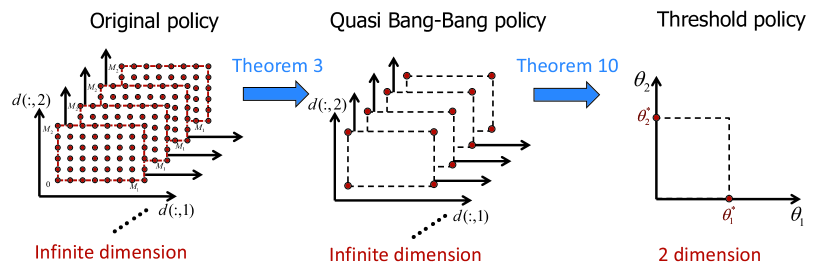
Figure 3: Illustration of policy space reduction with an example of 2-group server queue.

By utilizing the $c/{\mu}$-rule and the optimality of multi-threshold policy, we can further simplify Algorithm 1 to find the optimal threshold policy $\bm{\theta}^{*}$, which is described as Algorithm 2. We can see that Algorithm 2 iteratively updates the threshold policy $\bm{\theta}$. Consider two threshold policies $\bm{\theta}$ and $\bm{\theta}^{\prime}$ generated from two successive iterations, respectively, by using Algorithm 2. $d^{\prime}(n,k)$ and $d(n,k)$ are the associated scheduling action determined by (71) based on $\bm{\theta}^{\prime}$ and $\bm{\theta}$, respectively. From (71), we see that $d^{\prime}(n,k)$ and $d(n,k)$ have the following relation.

$$\begin{array}[]{ll}d^{\prime}(n,k)=d(n,k)=M_{k}\wedge\Big{(}n-\sum_{l=1}^{k-1}d(n,l)\Big{)},&\mbox{if }n\geq\theta_{k}^{\prime}\vee\theta_{k};\\ d^{\prime}(n,k)=d(n,k)=0,&\mbox{if }n<\theta_{k}^{\prime}\wedge\theta_{k};\\ d^{\prime}(n,k)=0,d(n,k)=M_{k}\wedge\Big{(}n-\sum_{l=1}^{k-1}d(n,l)\Big{)},&\mbox{if }(\theta_{k}^{\prime}\wedge\theta_{k}\leq n<\theta_{k}^{\prime}\wedge\theta_{k})\ \&\ (\theta_{k}^{\prime}>\theta_{k});\\ d(n,k)=0,d^{\prime}(n,k)=M_{k}\wedge\Big{(}n-\sum_{l=1}^{k-1}d^{\prime}(n,l)\Big{)},&\mbox{if }(\theta_{k}^{\prime}\wedge\theta_{k}\leq n<\theta_{k}^{\prime}\wedge\theta_{k})\ \&\ (\theta_{k}^{\prime}<\theta_{k}).\\ \end{array}$$ (73)

Substituting (73) into (28), we can derive the following performance difference formula that quantifies the effect of the change of threshold policy from $\bm{\theta}$ to $\bm{\theta}^{\prime}$, where $\bm{\theta},\bm{\theta}^{\prime}\in\mathbb{N}^{K}_{\uparrow}$.

$$\eta^{\prime}-\eta=\sum_{k=1}^{K}\sum_{n=\theta_{k}^{\prime}\wedge\theta_{k}}^{(\theta_{k}^{\prime}\vee\theta_{k})-1}\pi^{\prime}(n)\left(d^{\prime}(n,k)-d(n,k)\right)\left(c_{k}-\mu_{k}G(n)\right),$$ (74)

where $d^{\prime}(n,k)$ and $d(n,k)$ are determined by (73). From line 8-11 in Algorithm 2, we observe that once $G(n)$ is larger than $\frac{c_{k}}{\mu_{k}}$, we should set $\theta_{k}^{*}=n$ and turn on as many servers as possible in group $k$. Groups with smaller $\frac{c_{k}}{\mu_{k}}$ will be turned on with higher priority, which is the $c/\mu$-rule stated in Theorem 7. With performance difference formula (74), we see that the long-run average cost of the system will be reduced after each policy update in Algorithm 2. When the algorithm stops, it means that the system average cost cannot be reduced anymore and the optimal threshold $\bm{\theta}^{*}$ is obtained. This procedure is also similar to the policy iteration in the traditional MDP theory.

Algorithm 2 A $c/{\mu}$-rule based algorithm to find the optimal multi-threshold policy.

1:renumber the groups index in an ascending order of their value $\frac{c_{k}}{\mu_{k}}$, i.e., we have $\frac{c_{1}}{\mu_{1}}<\frac{c_{2}}{\mu_{2}}<\cdots<\frac{c_{K}}{\mu_{K}}$;

2:choose the initial threshold as $\bm{\theta}^{*}=(0,0,\cdots,0)_{K}$, which indicates to always turn on all servers;

3:repeat

4:     set $\bm{\theta}=\bm{\theta}^{*}$, $n=1$, and $k=1$;

5:     compute or estimate $\eta$ of the system under threshold policy $\bm{\theta}$;

6:     while $k\leq K$  do

7:         compute $G(n)$ by using (23) recursively or by solving (15) and (22);

8:         while ($G(n)>\frac{c_{k}}{\mu_{k}}$) $\&$ ($k\leq K$)  do

9:              set $\theta^{*}_{k}=n$;

10:              set $k=k+1$;

11:         end while

12:         set $n=n+1$;

13:     end while

14:until $\bm{\theta}=\bm{\theta}^{*}$ return optimal $\bm{\theta}^{*}$.

Comparing Algorithms 1 and 2, we observe that the essence of these two algorithms is similar: computing $G(n)$ and updating policies iteratively. However, Algorithm 2 is much simpler as it utilizes the $c/\mu$-rule based multi-threshold policy. The $c/\mu$-rule, as an optimal policy, is very easy to implement in practice. After the value of $G(n)$ is obtained, we compare it with the groups’ $\frac{c_{k}}{\mu_{k}}$ values. If $\frac{c_{k}}{\mu_{k}}$ is smaller, we should turn on as many servers as possible in group $k$; otherwise, turn off all servers in group $k$. Such a procedure will induce a multi-threshold type policy, as stated in Theorem 9.

More intuitively, we graphically demonstrate the above procedure by using an example in Fig. 4. The vertical axis represents the $c/{\mu}$ value of server groups, which are sorted in an ascending order. When $n$ increases and the system becomes more congested, we compute the value of the associated $G(n)$’s. As long as $G(n)$ is larger than $\frac{c_{k}}{\mu_{k}}$, we should turn on as many servers as possible for group $k$ and the associated $n$ is set as the threshold $\theta_{k}$. For the case of $n=6$, group 2 still has 1 server off although its $c/{\mu}$ is smaller than $G(n)$. It is because of Proposition 1 that the total number of working servers should not exceed $n$. Therefore, we can see that the $c/\mu$-rule will prescribe to turn on group servers from-bottom-up, as illustrated in Fig. 4. This example demonstrates the monotone structure of the $c/{\mu}$-rule and the optimal threshold policy.

Although Assumption 2 is reasonable for systems with non-human servers such as computers with different performance efficiencies (faster computers have smaller operating cost of processing each job), the scale economies may not exist in systems with human servers such as call centers where a faster server may incur much higher operating cost. Thus, it is necessary to investigate the robustness of the $c/\mu$-rule when Assumption 2 is not satisfied. This is done numerically by Example 6 in the next section.

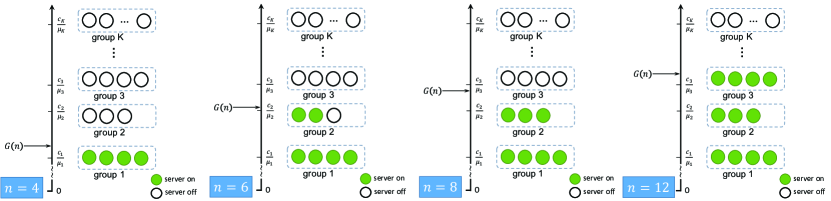
Figure 4: An example of $c/{\mu}$-rule to determine servers’ on-off, where groups are sorted in ascending order of their $c/{\mu}$ values.

5 Numerical Experiments

In this section, we conduct numerical experiments to verify the analytical results and gain useful insights about optimal policies.

5.1 Example 1: A general index policy case

First, we consider a system with 3 groups of servers. System parameters are as follows.

• Holding cost rate function: $h(n)=n$;

• Arrival rate: $\lambda=10$;

• Number of groups: $K=3$;

• Number of servers in groups: $\bm{M}=(M_{1},M_{2},M_{3})=(3,4,3)$;

• Service rates of groups: $\bm{\mu}=(6,4,2)$;

• Operating cost rates of groups: $\bm{c}=(7,4,3)$.

Note that Assumption 1 is satisfied since the holding cost rate function is $h(n)=n$ which is a linear function. However, Assumption 2 is not satisfied in this example as the descending order of $\bm{\mu}$ is different from the ascending order of ${c}/{\mu}$. Thus, the $c/{\mu}$-rule does not apply to this example. We use Algorithm 1 to find the optimal scheduling policy $d^{*}$ with the minimal average cost of $\eta^{*}=12.5706$. The average queue length $L$ (including customers in service) at each iteration is also illustrated along with the long-run average cost $\eta$ in Fig. 5(a). Since the holding cost function is $h(n)=n$, the long-run average holding cost is the same as $L$. Thus, the difference between $\eta$ and $L$ curves is the average operating cost. Note that $L$ significantly increases at the second iteration, which corresponds to a scenario with fewer servers working and more customers waiting. As shown in Fig. 5(a), the optimal solution is obtained after 4 iterations. We also plot the convex performance potential $g^{*}$ and the increasing PRF $G^{*}$ under the optimal policy $d^{*}$ in Fig. 5(b), as predicted in Theorems 4 and 5.

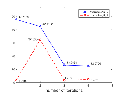
(a) Average cost and queue length during iterations.

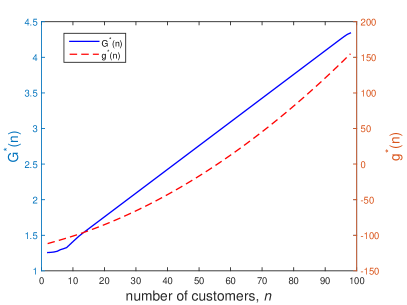
(b) Curves of $g^{*}$ and $G^{*}$.

Figure 5: Optimization procedure and curves of $g^{*}$ and $G^{*}$, $\lambda=10$, $K=3$, $\bm{M}=(3,4,3)$, $\bm{\mu}=(6,4,2)$, $\bm{c}=(7,4,3)$, $\eta^{*}=12.5706$.

The optimal scheduling policy is shown in Fig. 6(a) for the queue length up to 30 as the optimal actions for $n>30$ remain unchanged, as stated in Corollary 1 and Remark 2. In fact, the optimal action becomes $d^{*}(n)=(3,4,3)$, for any $n\geq 12$. The stair-wise increase in number of working servers for the short queue length range as shown in Fig. 6(a) reflects the fact that the optimal action should satisfy $d^{*}(n)\bm{1}\leq n$, as stated in Proposition 1. Note that Fig. 6(a) demonstrates that the optimal policy $d^{*}$ obeys the form of quasi bang-bang control defined in Theorem 3 and the number of total working servers $||d^{*}(n)||_{1}$ is increasing in $n$, as stated in Theorem 6.

However, the monotone property of $d^{*}(n,k)$ in Theorem 8 does not hold since Assumption 2 is not satisfied in this example. To demonstrate this point, we change the cost rate vector to $\bm{c}=(7,4,1.8)$ and keep other parameters the same as above. Using Algorithm 1, we obtain the optimal policy as illustrated in Fig. 6(b) after 5 iterations. We have $d^{*}(n)=(0,4,1)$ when $n=5$, while $d^{*}(n)=(2,4,0)$ when $n=6$. Therefore, we can see that the optimal policy of group 3, $d^{*}(n,3)$, is not always increasing in $n$. However, $||d^{*}(n)||_{1}$ is still increasing in $n$ which is consistent with Theorem 8.

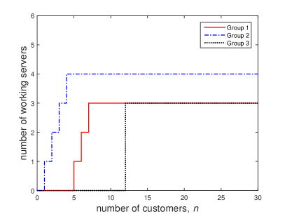
(a) Optimal policy with $\lambda=10$, $K=3$, $\bm{M}=(3,4,3)$, $\bm{\mu}=(6,4,2)$, $\bm{c}=(7,4,3)$, $\eta^{*}=12.5706$.

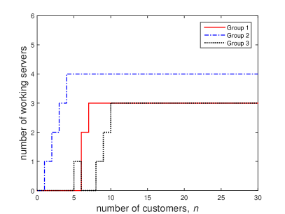
(b) Optimal policy with $\lambda=10$, $K=3$, $\bm{M}=(3,4,3)$, $\bm{\mu}=(6,4,2)$, $\bm{c}=(7,4,1.8)$, $\eta^{*}=12.5659$.

Figure 6: Optimal scheduling policies under different parameter settings.

5.2 Example 2: A $c/{\mu}$-rule case

We consider a system with the same set of parameters as that in the previous example except for the operating cost rates. Now we assume

• Operating cost rates of groups: $\bm{c}=(7,8,5)$.

With these new cost rates, the descending order of $\bm{\mu}$ is the same as the ascending order of $c/{\mu}$ of these groups, i.e., we have $\mu_{1}>\mu_{2}>\mu_{3}$ and $\frac{c_{1}}{\mu_{1}}<\frac{c_{2}}{\mu_{2}}<\frac{c_{3}}{\mu_{3}}$. Therefore, Assumption 2 is satisfied and the $c/{\mu}$-rule applies to this example. Thus, the optimal policy is a threshold vector $\bm{\theta}=(\theta_{1},\theta_{2},\theta_{3})$, as indicated by (71). We use Algorithm 2 to find the optimal threshold policy $\bm{\theta}^{*}$. From Fig. 7(a), we can see that after 5 iterations the optimal threshold policy is found to be $\bm{\theta}^{*}=(1,9,21)$ with $\eta^{*}=13.6965$. Comparing Examples 1 and 2, we note that both algorithms take around 4 or 5 iterations to converge, at a similar convergence speed. Algorithm 2 uses a threshold policy which only has 3 variables to be determined. However, the policy in Algorithm 1 is much more complex. Moreover, the $c/{\mu}$-rule significantly simplifies the search procedure in Algorithm 2. Fig. 7(b) illustrates the curves of $g^{*}(n)$ and $G^{*}(n)$, which are also consistent with the structures stated in Theorems 4 and 5.

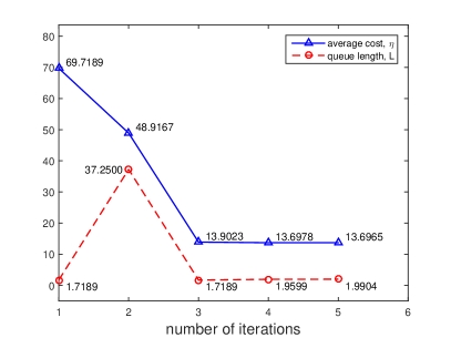
(a) Average cost and queue length during iterations.

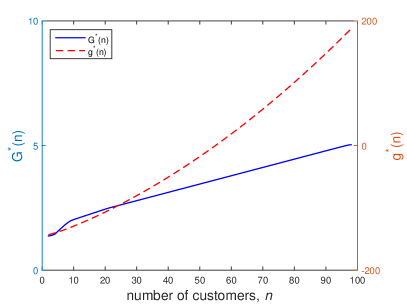
(b) Curves of $g^{*}$ and $G^{*}$.

Figure 7: Optimization procedure and curves of $g^{*}$ and $G^{*}$, $\lambda=10$, $K=3$, $\bm{M}=(3,4,3)$, $\bm{\mu}=(6,4,2)$, $\bm{c}=(7,8,5)$, $\eta^{*}=13.6965$.

5.3 Example 3: Effect of traffic intensity

We study the effect of traffic intensity on the optimal policy by varying the arrival rate $\lambda$ in Example 2. Since the maximal total service rate is $\sum_{k=1}^{K}M_{k}\mu_{k}=40$, we examine $0<\lambda<40$ range for the system stability. With $\lambda=[2\ 5\ 10\ 20\ 30\ 38\ 39]$, the optimal average cost $\eta^{*}$ and optimal thresholds are illustrated in Fig. 8(a) and Fig. 8(b), respectively. As the traffic intensity increases (the traffic becomes heavier), i.e., $\lambda\rightarrow 40$, the average cost $\eta^{*}$ will increase rapidly and the optimal threshold policy $\bm{\theta}^{*}$ converges to $(1,4,8)$, which means that servers are turned on as early as possible.

Note that the optimal threshold of the first group (its service rate is the largest) is always $\theta^{*}_{1}=1$ due to the zero setup cost, which is consistent with Theorem 10. It is expected that the optimal threshold $\theta^{*}_{1}$ could be other values if non-zero setup cost is considered.

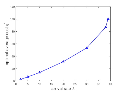
(a) Optimal average cost.

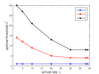
(b) Optimal thresholds.

Figure 8: Optimization results under different workloads with $\lambda=[2\ 5\ 10\ 20\ 30\ 38\ 39]$, $K=3$, $\bm{M}=(3,4,3)$, $\bm{\mu}=(6,4,2)$, $\bm{c}=(7,8,5)$.

5.4 Example 4: Trade-off of costs

For a system with the $c$/$\mu$-rule, the optimal threshold policy depends on the dominance between the holding cost and the operating cost. To study this effect on the optimal policy, we introduce an operating cost weight parameter $v$. The value of $v$ reflects the balance between the server provider’s operating cost and the customer’s waiting cost. In practice, $v$ depends on the system’s optimization objective. The cost rate function (4) is modified as below.

$$f(n,\bm{m})=h(n)+v\cdot\bm{m}\bm{c}.$$ (75)

Other parameters are the same as those in Example 2. Using Algorithm 2 and the set of operating cost weights $v=[0.1\ 0.3\ 0.5\ 1\ 2\ 3]$, we obtain the minimal average costs and the corresponding optimal threshold policies as shown in Fig. 9. The curve in Fig. 9(a) is almost linear, because the steady system mostly stays at states with small queue length and the associated part of $\eta^{*}$ is linear in $v$. When $v$ is small, it means that the holding cost $h(n)$ dominates the operating cost $\bm{m}\bm{c}$ in (75). Therefore, each server group should be turned on earlier (smaller thresholds) in order to avoid long queues. This explains why the optimal thresholds are $\bm{\theta}^{*}=(1,4,8)$ both for $v=0.1$ and $v=0.3$. When $v$ is large, the operating cost will dominate the holding cost. Thus, except for the first group (the most efficient group), the other two server groups are turned on only when the system is congested enough (larger thresholds).

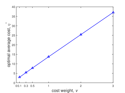
(a) Optimal average cost.

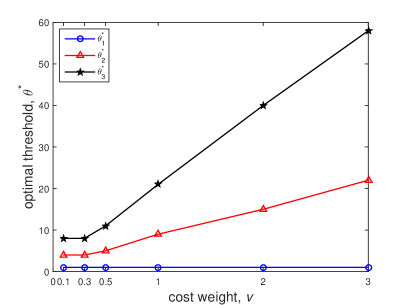
(b) Optimal thresholds.

Figure 9: Optimization results under different cost weights with $v=[0.1\ 0.3\ 0.5\ 1\ 2\ 3]$, $\lambda=10$, $K=3$, $\bm{M}=(3,4,3)$, $\bm{\mu}=(6,4,2)$, $\bm{c}=(7,8,5)$.

5.5 Example 5: Model scalability

Although all the previous examples are about small systems with only 3 server groups, our approach can be utilized to analyze large systems with many server groups and hundreds of servers. To demonstrate the model scalability, we consider a $c$/$\mu$-rule system (with scale economies) where $K$ increases as $[3\ 5\ 10\ 20\ 30\ 50]$. For the ease of implementation, we set $M_{k}=3$ for all $k$, $\bm{\mu}=(2,3,\cdots,K+1)$, and $\bm{c}=\bm{\mu}^{0.9}$ which indicates a component-wise power operation of $\bm{\mu}$. We can verify that this parameter setting satisfies the condition in Assumption 2. To keep the traffic intensity at a moderate level, we set $\lambda=0.5\cdot\bm{M}\bm{\mu}^{T}$, where $\bm{M}\bm{\mu}^{T}$ is the maximal total service rate of the system. The number of iterations of Algorithm 2 required for convergence is shown in Fig. 10 for different $K$ values. We find that the number of iterations remains almost stable (around 3 or 4) as the system size $K$ increases. This indicates the good scalability of our approach, namely, Algorithm 2 can be applied to a large scale system. Note that in our model the state space remains the same but the action space increases exponentially with $K$. Therefore, the optimal policy structure characterized (e.g. multi-threshold type) not only resolves the issue of infinite state space, but also the curse of dimensionality for action space.

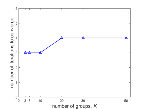
Figure 10: Number of iterations needed by Algorithm 2 under different problem scales with $K=[3\ 5\ 10\ 20\ 30\ 50]$, $\lambda=0.5\cdot\bm{M}\bm{\mu}^{T}$, $M_{k}\equiv 3$, $\bm{\mu}=(2,3,\cdots,K+1)$, $\bm{c}=\bm{\mu}^{0.9}$.

5.6 Example 6: Robustness of the $c/\mu$-rule

When the condition of scale economies in Assumption 2 does not hold, the optimality of the $c/\mu$-rule is not guaranteed. Since the $c/\mu$-rule is easy to implement, we investigate the robustness of the $c/\mu$-rule by numerically testing several scenarios where the condition of scale economies does not hold. For these cases, we first use Algorithm 1 to find the true optimal solution. Then, we use Algorithm 2 to find the “optimal” threshold policy as if the $c/\mu$-rule is applicable, i.e., servers in group with smaller $c/\mu$ will be turned on with higher priority. We obtain the following table to reveal the performance gaps between the optimal policy and the $c/\mu$-rule. The parameter setting is the same as that in Example 1, except that we choose different cost rate vectors $\bm{c}$ in different scenarios.

$\bm{c}$	$\eta^{*}$ by Algm.1	$\hat{\eta}^{*}$ by Algm.2	error
$[7,4,3]$	12.5706	12.5706	0.00%
$[7,4,1.8]$	12.5659	13.3287	6.07%
$[7,4,1]$	11.1580	11.1580	0.00%
$[8,3,1]$	10.0241	10.0615	0.37%
$[4,3,1]$	8.4044	9.2426	9.97%
$[18,10,3]$	23.4844	23.4844	0.00%

Table 1: The error effect of applying the $c/\mu$-rule when the condition of scale economies does not hold, $\lambda=10$, $K=3$, $\bm{M}=(3,4,3)$, $\bm{\mu}=(6,4,2)$.

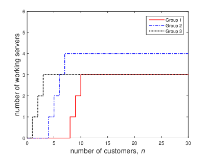
(a) Optimal policy by Algorithm 1 with $\bm{c}=(7,4,1)$, it is of threshold form with $\bm{\theta}^{*}=(8,4,1)$; “Optimal” threshold derived by Algorithm 2 is $\hat{\bm{\theta}}^{*}=(8,4,1)$; Their error is 0.00%.

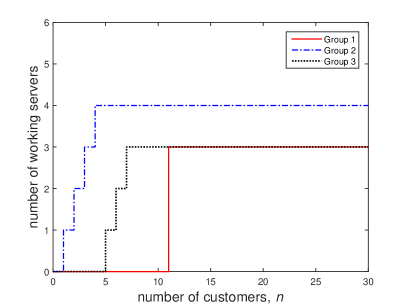
(b) Optimal policy by Algorithm 1 with $\bm{c}=(8,3,1)$, it is of threshold form with $\bm{\theta}^{*}=(11,1,5)$; “Optimal” threshold derived by Algorithm 2 is $\hat{\bm{\theta}}^{*}=(11,4,1)$; Their error is 0.37%.

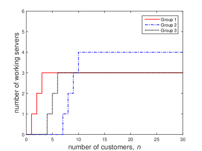
(c) Optimal policy by Algorithm 1 with $\bm{c}=(4,3,1)$, it is of threshold form with $\bm{\theta}^{*}=(1,7,4)$; “Optimal” threshold derived by Algorithm 2 is $\hat{\bm{\theta}}^{*}=(4,7,1)$; Their error is 9.97%.

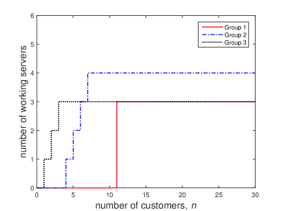
(d) Optimal policy by Algorithm 1 with $\bm{c}=(18,10,3)$, it is of threshold form with $\bm{\theta}^{*}=(11,4,1)$; “Optimal” threshold derived by Algorithm 2 is $\hat{\bm{\theta}}^{*}=(11,4,1)$; Their error is 0.00%.

Figure 11: Solutions derived by Algorithm 1 under different operating cost rate vectors with $\lambda=10$, $K=3$, $\bm{M}=(3,4,3)$, $\bm{\mu}=(6,4,2)$.

The first three cases in Table 1 are designed by changing two cost parameters from the original cost vector $\bm{c}=(7,8,5)$ used in Example 2 where the scale economies condition holds. We first change the operating cost of group 2 from 8 to 4 and the operating cost of group 3 from 5 to 3, 1.8, and 1, respectively, while other parameters are kept unchanged. Such parameter changes cause the $c/\mu$ ranking sequence to change from original $1\rightarrow 2\rightarrow 3$ to $2\rightarrow 1\rightarrow 3$, $3\rightarrow 2\rightarrow 1$, and $3\rightarrow 2\rightarrow 1$, respectively, for three server groups (from the fastest group 1 to slowest group 3). Note that in Case 1 (Example 1), the $c/\mu$ rankings switch between group 1 and group 2 with group 3 ranking unchanged so that the scale economies condition fails. However, the $c/\mu$-rule remains the optimal. This implies that a violation of the scale economies condition may not change the optimality of the $c/\mu$-rule. In Case 2, the $c/\mu$ ranking sequence becomes the reverse of the condition of scale economies and a cost gap of 6.07% occurs. It is interesting to see that in Case 3 a further cost reduction of group 3 will lead to the optimality of the $c/\mu$-rule again. For the next two cases, we keep the cost of group 3 at 1 while the costs of groups 1 and 2 are changed. It is found that the non-optimality of the $c/\mu$-rule in these cases will cause a less than 10% additional cost compared to the optimal index policy. Furthermore, it is still possible that the $c/\mu$-rule remains optimal for the reverse order of the scale economies condition as shown in Case 6.

Graphically, we can show how the optimal policy is different from the $c/\mu$-rule based threshold policy. The optimal server schedule derived by Algorithm 1 in Case 1 as shown in Fig. 6(a) is of threshold form with $\bm{\theta}^{*}=(5,1,8)$ which is the same as the “optimal” threshold derived by Algorithm 2. The optimal policy derived by Algorithm 1 in Case 2, which is not of threshold form, is shown in Fig. 6(b) while the “optimal” threshold derived by Algorithm 2 is $\hat{\bm{\theta}}^{*}=(8,4,1)$. Such a policy difference results in the performance degradation by 6.07%. For Case 3, the optimal solution derived by Algorithm 1 illustrated by Fig. 11(a) is of threshold form with $\bm{\theta}^{*}=(8,4,1)$ and the “optimal” threshold derived by Algorithm 2 is also $\hat{\bm{\theta}}^{*}=(8,4,1)$. These two solutions coincide and their performance error is 0. Other cases are illustrated by the sub-figures of Fig. 11 in a similar way.

Since $G(n)$ function plays a critical role in the optimality of the $c/\mu$-rule and depends on multiple system parameters, we cannot develop a pattern for the optimality of $c/\mu$-rule when the condition of scale economies does not hold. However, from Table 1 and Fig. 11, we observe that in some cases, although the condition of scale economies does not hold, the optimality of the $c/\mu$-rule still holds. In other cases, the performance degradation caused by “faultily” using the $c/\mu$-rule is tolerable. This implies that the $c/\mu$-rule has a good applicability and robustness, even for the cases where the condition of scale economies does not hold.

6 Conclusion

In this paper, we study the service resource allocation problem in a stochastic service system, where servers are heterogeneous and classified into groups. Under a cost structure with customer holding and server operating costs, we investigate the optimal index policy (dynamic scheduling policy) which prescribes the number of working servers in each group at each possible queue length. Using the SBO theory, we characterize the structure of the optimal policy as a quasi bang-bang control type. A key technical result of this work is to establish the monotone increasing property of PRF $G^{*}(n)$, a quantity that plays a fundamental role in the SBO theory. Then, the necessary and sufficient condition and the monotone property of the optimal policy are derived based on this property. Under an assumption of scale economies, we further characterize the optimal policy as the $c/\mu$-rule. That is, the servers in group with smaller $c/\mu$ should be turned on with higher priority. The optimality of multi-threshold policy is also proved. These optimality structures significantly reduce the complexity of the service resource allocation problem and resolve the issue of curse of dimensionality in a more general heterogeneous multi-server queueing model with infinite state space. Based on these results, we develop the efficient algorithms for computing the optimal scheduling policy and thresholds. Numerical examples demonstrate these main results and reveal that the $c/\mu$-rule has a good scalability and robustness.

A limitation of our model is that the startup and shutdown cost of each server is assumed to be zero. The cost of customer migration among servers is also neglected. Taking these costs into account in our model can be a future research topic. Moreover, we assume linear operating costs in this paper. It would be interesting to extend our results to a more general operating cost structure. Asymptotically extending to the scenario of many servers in a networked setting under the fluid regime can also be another future research direction.

References

- [1] O. T. Akgun, D. G. Down, and R. Righter, “Energy-aware scheduling on heterogeneous processors,” IEEE Trans. Automatic Control, vol. 59, no. 3, pp. 599-613, 2014.
- [2] M. Armony and A. R. Ward, “Fair dynamic routing in large-scale heterogeneous-server systems,” Oper. Res., vol. 58, no. 3, pp. 624-637, 2010.
- [3] R. Atar, C. Giat, and N. Shimkin, “The rule for many-server queues with abandonment,” Oper. Res., vol. 58, no.5, pp. 1427-1439, 2010.
- [4] K. R. Balachandran and H. Tijms, “On the D-policy for the M/G/1 queue,” Management Sci., vol. 21, pp. 1073-1076, 1975.
- [5] J. S. Baras, A. J. Dorsey, and A. M. Makowski, “Two competing queues with linear costs: The -rule is often optimal,” Adv. Appl. Prob., vol. 17, pp. 186-209. 1985.
- [6] J. S. Baras, D.-J. Ma, and A. Makowski, “ competing queues with geometric service requirements and linear costs: The -rule is always optimal,” Syst. Control Lett., vol. 6, no.3, pp. 173-180, 1985.
- [7] C. E. Bell, “Optimal operation of an M/M/2 queue with removable servers,” Oper. Res., vol. 28, no. 5, pp. 1189-1204, 1980.
- [8] C. Buyukkoc, P. Varaiya, and J. Walrand, “The -rule revisited,” Adv. Appl. Probab., vol. 17, pp. 237-238, 1985.
- [9] X. R. Cao, Realization Probabilities: The Dynamics of Queueing Systems. Springer-Verlag, New York, 1994.
- [10] X. R. Cao, Stochastic Learning and Optimization – A Sensitivity-Based Approach. New York: Springer, 2007.
- [11] F. De Vericourt and Y. P. Zhou, “On the incomplete results for the heterogeneous server problem,” Queueing Systems, vol. 52, pp. 189-191, 2006.
- [12] A. B. Dieker, S. Ghosh, and M. S. Squillante, “Optimal resource capacity management for stochastic networks,” Oper. Res., vol. 65, no. 1, pp. 221-241, 2017.
- [13] M. C. Fu, S. I. Marcus, and I. Wang, “Monotone optimal policies for a transient queueing staffing problem,” Oper. Res., vol. 48, no. 2, pp. 327-331, 2000.
- [14] J. Fu, B. Moran, J. Guo, E. W. M. Wong, and M. Zukerman, “Asymptotically optimal job assignment for energy-efficient processor-sharing server farms,” IEEE J. Sel. Areas Commun., vol. 34, no. 12, pp. 4008-4023, 2016.
- [15] A. Gandhi, V. Gupta, M. Harchol-Balter, and M. A. Kozuch, “Optimality analysis of energy-performance trade-off for server farm management,” Performance Eval., vol. 67, no. 11, pp. 1155-1171, 2010.
- [16] J. C. Gittins, K. Glazebrook, and R. Weber. Multi-Armed Bandit Allocation Indices. Wiley, 2011.
- [17] R. Hassin, “On the optimality of first-come last-served queues,” Econometrica, vol. 53, pp. 201-202, 1985.
- [18] R. Hassin and M. Haviv. To Queue or Not to Queue: Equilibrium Behavior in Queueing Systems, Springer, 2003.
- [19] R. Hassin, Y. Y. Shaki, and U. Yovel, “Optimal service-capacity allocation in a loss system,” Nav. Res. Logist., vol. 62, pp. 81-97, 2015.
- [20] D. P. Heyman, “Optimal operating policies for M/G/1 queuing systems,” Oper. Res., vol. 16, pp. 362-382, 1968.
- [21] D. P. Heyman, “The T-policy for the M/G/1 queue,” Management Sci., vol. 23, pp. 775-778, 1977.
- [22] Y. C. Ho and X. R. Cao, Perturbation Analysis of Discrete-Event Dynamic Systems. Kluwer Academic Publisher, Boston, 1991.
- [23] T. Hirayama, M. Kijima, and S. Nishimura, “Further results for dynamic scheduling of multiclass G/G/l queues,” J. Appl. Probab., vol. 26, pp. 595-603, 1989.
- [24] Z. Hua, W. Chen, and Z. G. Zhang, “Competition and coordination in two-tier public service systems under government fiscal policy,” Prod. Oper. Manag., vol. 25, no. 8, pp. 1430-1448, 2016.
- [25] K. Kant, “Data center evolution: A tutorial on state of the art, issues, and challenges,” Comput. Netw., vol. 53, no. 17, pp. 2939-2965, 2009.
- [26] A. Kebarighotbi and C. G. Cassandras, “Optimal scheduling of parallel queues using stochastic flow models,” Discrete Event Dyn. S., vol. 21, pp. 547-576, 2011.
- [27] G. P. Klimov, “Time-sharing service systems,” Theory Probab. Appl., vol. 19, no. 3, pp. 532-551, 1974.
- [28] D. Kumar, T. C. Aseri, and R. B. Patel, “EEHC: Energy efficient heterogeneous clustered scheme for wireless sensor networks,” Comput. Commun., vol. 32, no. 4, pp. 662-667, 2009.
- [29] Q. L. Li and J. Cao, “Two types of RG-factorizations of quasi-birth-and-death processes and their applications to stochastic integral functionals,” Stoch. Models, vol. 20, no. 3, 299-340, 2004.
- [30] Q. L. Li, J. Y. Ma, M. Xie, and L. Xia, “Group-server queues,” W. Yue et al. (Eds.): Proc. QTNA’2017, LNCS 10591, pp. 49-72, 2017.
- [31] W. Lin and P. Kumar, “Optimal control of a queueing system with two heterogeneous servers,” IEEE Trans. Automatic Control, vol. 29, no. 8, pp. 696-703, 1984.
- [32] H. Luh and I. Viniotis, “Threshold control policies for heterogeneous server systems,” Math. Meth. Oper. Res., vol. 55, no. 1, pp. 121-142, 2002.
- [33] D. J. Ma and X. R. Cao, “A direct approach to decentralized control of service rates in a closed Jackson network,” IEEE Trans. Automatic Control, vol. 39, no. 7, pp. 1460-1463, 1994.
- [34] A. Mandelbaum and A. L. Stolyar, “Scheduling flexible servers with convex delay costs: Heavy-traffic optimality of the generalized -rule,” Oper. Res., vol. 52, pp. 836-855, 2004.
- [35] W. P. Millhiser, C. Sinha, and M. J. Sobel, “Optimality of the fastest available server policy,” Queueing Systems, vol. 84, pp. 237-263, 2016.
- [36] P. Nain and D. Towsley, “Optimal scheduling in a machine with stochastic varying processing rate,” IEEE Trans. Automatic Control, vol. 39, no. 9, pp. 1853-1855, 1994.
- [37] M. L. Puterman, Markov Decision Processes: Discrete Stochastic Dynamic Programming. New York: John Wiley & Sons, 1994.
- [38] Z. Rosberg, P. P. Varaiya, and J. C. Walrand, “Optimal control of service in tandem queues,” IEEE Trans. Automatic Control, vol. 27, pp. 600-609, 1982.
- [39] V. V. Rykov, “Monotone control of queueing systems with heterogeneous servers,” Queueing Systems, vol. 37, pp. 391-403, 2001.
- [40] S. Saghafian and M. H. Veatch, “A rule for two-tiered parallel servers,” IEEE Trans. Automatic Control, vol. 61, no. 4, pp. 1046-1050, 2016.
- [41] W. E. Smith, “Various optimizers for single-stage production,” Nav. Res. Logist. Quart., vol. 3, pp. 59-66, 1956.
- [42] M. J. Sobel, “Optimal average-cost policy for a queue with start-up and shut-down costs,” Oper. Res., vol. 17, pp. 145-162, 1969.
- [43] S. Stidham and R. Weber, “A survey of Markov decision models for control of networks of queues,” Queueing Systems, vol. 13, pp. 291-314, 1993.
- [44] N. Tian and Z. G. Zhang, Vacation Queueing Models – Theory and Applications. Springer, New York, 2006.
- [45] J. N. Tsitsiklis and K. Xu, “Flexible Queueing Architecture,” Oper. Res., vol. 65, no. 5, pp. 1398-1413, 2017.
- [46] B. Urgaonkar, G. Pacifici, P. Shenoy, M. Spreitzer, and A. Tantawi, “An analytical model for multi-tier Internet services and its applications,” Proc. 2005 ACM SIGMETRICS, Jun. 6-10, 2005, Banff, Alberta, Canada, pp. 291-302.
- [47] J. A. Van Mieghem, “Dynamic scheduling with convex delay costs: The generalized rule,” Ann. Appl. Prob., vol. 5, no. 3, pp. 809-833, 1995.
- [48] J. A. Van Mieghem, “Due-date scheduling: Asymptotic optimality of generalized longest queue and generalized largest delay rules,” Oper. Res., vol. 51. no. 1, pp. 113-122, 2003.
- [49] J. Walrand, “A note on ‘optimal control of a queueing system with two heterogeneous servers’,” Syst. Control Lett., vol. 4, pp. 131-134, 1984.
- [50] H. Wang and P. Varman, “Balancing fairness and efficiency in tiered storage systems with bottleneck-aware allocation,” Proc. 12th USENIX Conf. File and Storage Technologies (FAST’14), Feb. 17-20, 2014, Santa Clara, CA, USA, pp. 229-242.
- [51] A. R. Ward and M. Armony, “Blind fair routing in large-scale service systems with heterogeneous customers and servers,” Oper. Res., vol. 61, no. 1, pp. 228-243, 2013.
- [52] R. R. Weber, “On a conjecture about assigning jobs to processors of different speeds,” IEEE Trans. Automatic Control, vol. 38, no. 1, pp. 166-170, 1993.
- [53] R. R. Weber and S. Stidham, “Optimal control of service rates in networks of queues,” Adv. Appl. Probab., vol. 19, pp. 202-218, 1987.
- [54] P. Whittle, “Restless bandits: Activity allocation in a changing world,” J. Appl. Probab., vol. 25, pp. 287-298, 1988.
- [55] L. Xia, “Service rate control of closed Jackson networks from game theoretic perspective,” Eur. J. Oper. Res., vol. 237, no. 2, pp. 546-554, 2014.
- [56] L. Xia and B. Shihada, “Max-Min optimality of service rate control in closed queueing networks,” IEEE Trans. Automatic Control, vol. 58, pp. 1051-1056, 2013.
- [57] L. Xia and Q. S. Jia, “Parameterized Markov decision process and its application to service rate control,” Automatica, vol. 54, pp. 29-35, 2015.
- [58] S. H. Xu and J. G. Shantikumar, “Optimal expulsion control – A dual approach to admission control of an ordered-entry system,” Oper. Res., vol. 41, pp. 1137-1152, 1993.
- [59] M. Yadin and P. Naor, “Queuing systems with a removable service station,” Oper. Res. Quart., vol. 14, pp. 393-405, 1963.
- [60] D. D. Yao and Z. Schechner, “Decentralized control of service rates in a closed Jackson network,” IEEE Trans. Automatic Control, vol. 34, no. 2, pp. 236-240, 1989.
- [61] J. Yoo, Queueing Models for Staffing Service Operations, Ph.D. dissertation, University of Maryland, College Park, 1996.
- [62] Z. G. Zhang, “Performance analysis of a queue with congestion-based staffing policy,” Management Sci., vol. 55, no. 2, pp. 240-251, 2009.
- [63] G. Zhang, L. Chiu, and L. Liu, “Adaptive data migration in multi-tiered storage based cloud environment,” Proc. 2010 IEEE International Conf. on Cloud Computing (CLOUD’10), Jul. 5-10, 2010, Miami, FL, USA, pp. 148-155.