Dispersion in two-dimensional periodic channels with discontinuous profiles

Abstract

The effective diffusivity of Brownian tracer particles confined in periodic micro-channels is smaller than the microscopic diffusivity due to entropic trapping. Here, we study diffusion in two-dimensional periodic channels whose cross-section presents singular points, such as abrupt changes of radius or the presence of thin walls, with openings, delimiting periodic compartments composing the channel. Dispersion in such systems is analyzed using the Fick-Jacobs’ approximation. This approximation assumes a much faster equilibration in the lateral than in the axial direction, along which the dispersion is measured. If the characteristic width $a$ of the channel is much smaller than the period $L$ of the channel, i.e. $\varepsilon=a/L$ is small, this assumption is clearly valid for Brownian particles. For discontinuous channels, the Fick-Jacobs’ approximation is only valid at the lowest order in $\varepsilon$ and provides a rough, though on occasions rather accurate, estimate of the effective diffusivity. Here we provide formulas for the effective diffusivity in discontinuous channels that are asymptotically exact at the next-to-leading order in $\varepsilon$. Each discontinuity leads to a reduction of the effective diffusivity. We show that our theory is consistent with the picture of effective trapping rates associated with each discontinuity, for which our theory provides explicit and asymptotically exact formulas. Our analytical predictions are confirmed by numerical analysis. Our results provide a precise quantification of the kinetic entropic barriers associated with profile singularities.

Introduction

Characterizing the dispersion of random walkers in complex heterogeneous media is an important issue that appears in contexts as various as mixing Le Borgne, Dentz, and Villermaux (2013); Dentz et al. (2011); Barros et al. (2012), sorting Bernate and Drazer (2012), contaminant spreading Brusseau (1994); Dean et al. (2007) and diffusion controlled reactions Condamin et al. (2007). In particular, the dispersion of Brownian particles in channels is a paradigm for diffusion in confined and crowded environments such as biological cells, zeolites, porous media, ion channels and microfluidic devices Burada et al. (2009); Malgaretti, Pagonabarraga, and Rubi (2013); Bressloff and Newby (2013); Holcman and Schuss (2013). The relation between confining geometry and effective diffusivity has been extensively investigated in the physics and chemistry literature over the last decade Yang et al. (2017); Burada et al. (2008); Reguera et al. (2006); Kalinay and Percus (2006); Malgaretti, Pagonabarraga, and Rubi (2013); Malgaretti, Pagonabarraga, and Miguel Rubi (2016); Yang et al. (2017). One of the most popular theoretical approaches to diffusion in channels is the so-called Fick-Jacobs’ (FJ) approximation Jacobs (1967), based on a dimensional reduction. In the case of two-dimensional channels of local radius $R(x)$, with $x$ the coordinate in the longitudinal direction, the FJ approach reduced the study of tracer dispersion to that of an effective one-dimensional particle, with position $x(t)$, diffusing in an effective entropic potential $\phi(x)=-k_{B}T\ln R(x)$. In symmetric periodic channels, the late-time effective diffusivity $D_{e}$ for this one-dimensional problem can then be deduced from the Lifson-Jackson formulaLifson and Jackson (1962),

$$D_{e}\simeq D_{\mathrm{FJ}}=\frac{D_{0}}{\langle R\rangle\langle R^{-1}\rangle},$$ (1)

where $D_{0}$ is the microscopic diffusivity, and $\langle R\rangle=\int_{0}^{L}dxR(x)/L$ denotes the uniform average over the channel period $L$.

This basic FJ approximation is valid when the typical equilibration time in the lateral direction is much smaller than the characteristic time scale of the dynamics in the longitudinal direction. This means that the FJ expression (1) can be seen as the leading order term of an expansion of $D_{e}$ in powers of the small parameter $\varepsilon\equiv a/L$, where $a$ is the typical lateral channel width . For non-vanishing $\varepsilon$, FJ theories can be made more accurate by introducing a position dependent local diffusion coefficient $D(x)$ in the effective one-dimensional description Zwanzig (1992); Reguera and Rubi (2001); Kalinay and Percus (2006, 2005a, 2005b, 2010); Martens et al. (2011); Bradley (2009); Berezhkovskii and Szabo (2011); Dagdug and Pineda (2012); Valdes and Guzman (2014). At next-to-leading order, $D(x)\simeq D_{0}(1-R^{\prime 2}/3)$ Zwanzig (1992); Reguera and Rubi (2001); Kalinay and Percus (2006), leading (again using the Lifson-Jackson formulaLifson and Jackson (1962)) to

$$D_{e}\simeq\frac{D_{0}}{\langle R\rangle\langle R^{-1}\rangle}\left(1-\frac{\langle R^{\prime 2}/R\rangle}{3\langle R^{-1}\rangle}+\mathcal{O}(\varepsilon^{4})\right),$$ (2)

where the prime denotes the derivative with respect to $x$. For smooth channels, it has been checkedDorfman and Yariv (2014); Mangeat, Guérin, and Dean (2017a) that the above formula is exact at order $\varepsilon^{2}$, and it can be extended to higher orders Kalinay and Percus (2006); Dorfman and Yariv (2014); Mangeat, Guérin, and Dean (2017a). However, in the case of channel profiles presenting a discontinuity, it is straightforward to see that the next order correction to the dispersivity $D_{e}$ given in Eq. (2) diverges. The appearance of such a divergence usually suggests two possibilities. Firstly it could be that the basic perturbation series needs to be resummed, for instance, on resummation, divergent terms appear in a denominator rather than a numerator and thus give finite contributions. The other possibility is that the true perturbation series is not analytic in the naive expansion parameter, which in the approaches mentioned above turns out to be $\varepsilon^{2}$. In our study we show that it is the latter phenomenon which is at play and that the perturbation expansion parameter is in fact $\varepsilon$ rather than $\varepsilon^{2}$.

To treat this problem, existing approaches assume that the effective dynamics for $x(t)$ should include local traps at the points of discontinuity, the associated trapping rates are calculated approximately via the boundary homogenization approximationBerezhkovskii, Barzykin, and Zitserman (2009); Antipov et al. (2013). RecentlyKalinay and Percus (2010), this theory has been found to be consistent with the approaches assuming a local diffusivity $D(x)$. However, the effective dispersivity contains coefficients which not known in explicitly. In a third class of approaches, dispersion has been estimated by using first passage argumentsMarchesoni (2010); Borromeo and Marchesoni (2010), which is valid in the limit of small openings between pores, but whose link with the FJ regime is unclearMangeat, Guérin, and Dean (2017b).

The aim of the present paper is to derive a formula for the effective dispersion in discontinuous channels that is asymptotically exact in the slowly varying limit $\varepsilon\to 0$. We consider two dimensional periodic channels which possess a finite number $n$ of discontinuities in each period. Our main result is that the dispersion in such channels can be written as

$$D_{e}\simeq\frac{D_{0}}{\langle R\rangle\langle R^{-1}\rangle}\left(1-\sum_{i=1}^{n}\frac{\mu_{i}}{L\langle R^{-1}\rangle}+\mathcal{O}(\varepsilon^{2})\right).$$ (3)

Here, the positive coefficients $\mu_{i}$ only depend on the geometry of the $i^{\mathrm{th}}$ discontinuity (see below). Furthermore the effect of each distinct discontinuity is additive and thus the result applies to a wide range of channels in a simple, building block, like manner. The above formula generalizes Eq. (2) to the case of discontinuous profiles, and shows that the associated corrections to dispersion are of order $\varepsilon$, and are as such thus much more important than for smooth channels (where they are of order $\varepsilon^{2}$). Importantly, our approach does not rely on a reduction of dimensionality: we do not need to define a local diffusion coefficient near the singular parts of the channel to obtain it, such local diffusion coefficient would clearly be ill-defined near the profile discontinuity. Our analysis is however compatible with the notion of associated trapping rates to model the singularity, and provides a means to obtain asymptotically exact formulas for such trapping rates, which are shown to be proportional to $1/\mu$.

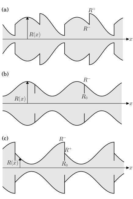
Figure 1: Illustration of the three types of discontinuities of periodic channels that are considered in this paper: (a) discontinuity of the channel radius, (b) presence of walls separating between compartments and (c) general case composed by both type of discontinuities.

Our formula (3) shows that each discontinuity has a negative contribution to the dispersion, confirming that it effectively acts as a local trap for the Brownian particles. We have exactly calculated the coefficients $\mu$, that quantify the impact on dispersion, for two different types of basic discontinuities, shown in Fig. 1. First, we have considered the case where the channel radius changes locally from a value $R^{-}$ to $R^{+}$ (see Fig. 1a). In this case, $\mu$ is denoted by $\mu_{d}$ (where $d$ stands for discontinuous) and depends only on the parameter $\nu=R^{+}/R^{-}$:

$$\mu_{d}(\nu)=\frac{1+\nu^{2}}{\nu\ \pi}\ln\left|\frac{1+\nu}{1-\nu}\right|-\frac{2}{\pi}\ln\left|\frac{4\nu}{1-\nu^{2}}\right|.$$ (4)

Notice that $\mu_{d}(\nu)=\mu_{d}(\nu^{-1})$, this must be the case as we have the same diffusion constant upon flipping the direction of the channel and thus switching $R^{+}$ and $R^{-}$. We have also considered a second type of discontinuity, in which the profile contains walls that partially obstruct the channel, forming different compartments (see Fig. 1b). In this case, $\mu$ is denoted by $\mu_{c}$ ($c$ standing for compartments) and depends on the geometric parameter $\nu=R_{0}/R^{-}$ (where $R_{0}$ is the radius at minimal opening and $R^{-}$ is the radius just next the wall), and is given by

$$\mu_{c}(\nu)=-\frac{4}{\pi}\ln\left(\sin\frac{\pi\nu}{2}\right).$$ (5)

Both functions $\mu_{c}$ and $\mu_{d}$ are plotted in Fig. 2. We also consider a hybrid case where the discontinuity is a combination of these type of discontinuities.

The outline of this paper is as follows. In Section I we present the general formalism used and show that the effective diffusivity can be computed via a partial differential equation for an auxiliary function over one channel period. In Section II, we consider discontinuous channels. We present a method to compute this auxiliary function with matched asymptotic expansions and we compute the effective diffusivity. In Section III.1, we show how to adapt the calculation for compartmentalized channels and in Section III.2 we generalize the result to systems having hybrid forms of the discontinuous and compartmentalized singularities. Our formulas are validated by comparison with the numerical solutions of the relevant partial differential equations in Section IV. In Section V, we determine the exact expressions for the of the trapping rates that should be used for the boundary homogenization method, and compare them with existing approximations.

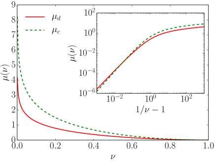
Figure 2: Representation of the function $\mu(\nu)$ which quantifies the impact on dispersion of the presence of a radius discontinuity ($\mu_{c}$) or of a partially obstructing wall delimiting compartments ($\mu_{d}$). The geometric parameter is $\nu=R^{-}/R^{+}$ for discontinuous channels and $\nu=R^{-}/R_{0}$ for compartmentalized channels, where $R^{-}$, $R_{0}$ and $R^{+}$ are as shown in Fig. 1.

I General formalism: exact expression of the effective diffusivity

We consider a symmetric two-dimensional channel of local radius $R(x)$, where $x$ denotes the longitudinal coordinate. The channel is periodic in $x$ with period $L$. We denote by $a$ the channel width at its minimum, and we define the dimensionless profile $\zeta$ by

$$R(x)=a\ \zeta(x/L),$$ (6)

where $\zeta(X)$ is a periodic function of $X=x/L$, with unit period, that describes the geometry of the profile.

We aim to calculate the effective diffusivity

$$D_{e}=\underset{t\rightarrow\infty}{\lim}\overline{[x(t)-x(0)]^{2}}/2t,$$ (7)

where $\overline{\ \cdot\ }$ represents the ensemble average over particle trajectories. Rather than reducing the problem to an effective one-dimensional dynamics for $x(t)$, we use the following exact expression of the effective diffusivityGuérin and Dean (2015a, b); Mangeat, Guérin, and Dean (2017a)

$$\frac{D_{e}}{D_{0}}=1-\frac{1}{|V|}\int_{\partial V}dS\ n_{x}\ f.\$$ (8)

Here, the integral is performed on the boundary $\partial V$ of the channel (over one periodic cell), $D_{0}$ is the microscopic diffusivity, $dS$ represents the surface element, $n_{x}$ is the $x$ component of the unit normal vector $\mathbf{n}$ (oriented towards the exterior of the channel), $|V|=2\langle R\rangle L$ is the volume of one channel period. Furthermore, $D_{e}$ depends on an auxiliary function $f(x,y)$ which satisfies the Laplace equation

$$\nabla^{2}f=\partial_{x}^{2}f+\partial_{y}^{2}f=0,$$ (9)

where $y$ is the transverse coordinate. In addition. $f$ is a periodic function of $x$, and at the channel boundary it obeys the boundary condition

$$[\mathbf{n}\cdot\nabla f-n_{x}]_{y=\pm R(x)}=0.$$ (10)

The above expressions are a particular case of the formulas for the effective diffusivity for general periodic systemsGuérin and Dean (2015a, b), and are also consistent with the macrotransport theory of Brenner and Edwards Brenner and Edwards (1993). An important dimensionless parameter of the problem is the ratio of lateral to longitudinal length scales

$$\varepsilon=a/L$$ (11)

and we will study the limit of slowly varying channels, i.e. $\varepsilon\to 0$. For smooth channels, $D_{e}$ can be systematically expressed as an expansion in powers of $\varepsilon$. Here we focus on non-smooth channels, for which only the leading order result is exactly known [Eq. (1)].

To simplify notation, without loss of generality, we set the period length to $L=1$ and the microscopic diffusivity to $D_{0}=1$. In these units, $\varepsilon$ is just the typical lateral dimension of the channel, and $R=\varepsilon\zeta$.

II Dispersion in weakly-varying discontinuous channels

Here, we first consider the case that $\zeta(x)$ presents a single discontinuity, whose origin is set at the origin $x=0$ (modulo the period). There, $\zeta(x)$ is assumed to change sharply from $\zeta^{-}\equiv\zeta(0^{-})$ to $\zeta^{+}\equiv\zeta(0^{+})$, as in Fig. 1a. In the slowly-varying limit $\varepsilon\to 0$, characterizing $f$ is a singular perturbation problem, and it is crucial to distinguish between a region near the channel discontinuity (called the inner region), and a region far from the discontinuity (called the outer region).

II.1 The solution far from the discontinuity

We first describe the expansion of $f$ in the outer region, where it is convenient to use the rescaled variables

$$Y=y/\varepsilon,\hskip 28.45274ptX=x,$$ (12)

so that the ranges of $X,Y$ become independent of $\varepsilon$. We define the function $F$ such that

$$f(x,y)=F(X,Y).$$ (13)

It is important to note that $F$ is periodic but may present an irregular behavior (to be determined below) near the discontinuity, at $X=0$ (modulo 1). The equation satisfied by $F$ in the bulk follows from Eq. (9),

$$\varepsilon^{2}\partial_{X}^{2}F+\partial_{Y}^{2}F=0,$$ (14)

and the boundary conditions Eq. (10) become

$$[\varepsilon^{2}\zeta^{\prime}(X)\partial_{X}F-\partial_{Y}F]_{Y=\pm\zeta(X)}=\varepsilon^{2}\zeta^{\prime}(X).$$ (15)

In the limit $\varepsilon\rightarrow 0$, we look for solutions of the form

$$F(X,Y)=\sum_{i=0}^{\infty}\varepsilon^{i}F_{i}(X,Y).$$ (16)

Note that here it is essential to use $\varepsilon$ as the small parameter, and not $\varepsilon^{2}$ which is the relevant small parameter used to study smooth channelsDorfman and Yariv (2014).

Inserting this series expansion into the above equations leads to recurrence equations for the functions $F_{i}$. This calculation is very similar to the approach presented by Dorfman and YarivDorfman and Yariv (2014), and the details are given in Appendix A. At leading order, we find

$$F_{0}^{\prime}(X)=1-\frac{1}{\langle\zeta^{-1}\rangle\zeta(X)}.$$ (17)

At next order, we find that $F_{1}$ is discontinuous at $0$ (and hence at $1$ by periodicity) and its derivative is given by

$$F_{1}^{\prime}(X)=\frac{F_{1}(0^{-})-F_{1}(0^{+})}{\langle\zeta^{-1}\rangle\zeta(X)}.$$ (18)

The unknown value of the jump $F_{1}(0^{-})-F_{1}(0^{+})$ will be deduced from the matching condition with the inner solution in the next section.

II.2 The solution near the discontinuity

We now consider the function $f$ near the channel discontinuity (located at $X=0$ modulo $1$). In this region, the relevant length scale for the transverse direction is the channel width $\sim\varepsilon$. Since the change of profile is abrupt, we expect that $f$ varies with the same length scale in the longitudinal direction. This suggests that the relevant variables in the inner region are $\tilde{x}$ and $\tilde{y}$ defined by

$$\tilde{x}=x/\varepsilon=X/\varepsilon,\hskip 28.45274pt\tilde{y}=y/\varepsilon=Y.$$ (19)

We note that, if $|x|\ll 1$, one can simplify the domain by noting that $R(x)\simeq\varepsilon\zeta^{+}$ for $x>0$, and $R(x)\simeq\varepsilon\zeta^{-}$ for $x<0$. It is convenient to introduce the function $\phi$, defined by

$$\phi(\tilde{x},\tilde{y})=f(x,y)-x.$$ (20)

This function $\phi$ satisfies the Laplace’s equation,

$$(\partial_{\tilde{x}}^{2}+\partial_{\tilde{y}}^{2})\phi=0,$$ (21)

and it follows from Eq. (10) that Neumann conditions $\mathbf{n}\cdot\tilde{\nabla}\phi=0$ hold at the channel boundary. We again look for an expansion of the form

$$\phi(\tilde{x},\tilde{y})=\phi_{0}(\tilde{x},\tilde{y})+\varepsilon\phi_{1}(\tilde{x},\tilde{y})+...$$ (22)

As a result all the functions $\phi_{i}$ satisfy Laplace’s equation with Neumann boundary conditions at the channel boundary, but an additional condition is needed to determine them. This additional condition comes from the requirement that both expansions (16) and (22) must lead to the same value of $f$ when $\varepsilon\ll|x|\ll 1$. Thus the value of $F$ for small $X$ must be equal to $x+\phi$ when $\tilde{x}\rightarrow\pm\infty$. This condition can be written explicitly as

$$\phi+\varepsilon\tilde{x}\underset{\tilde{x}\rightarrow\pm\infty}{\simeq}F_{0}(0)+\varepsilon[\tilde{x}F_{0}^{\prime}(0^{\pm})+F_{1}(0^{\pm})]+...$$ (23)

At leading order in $\varepsilon$, the above equations imply that $\phi_{0}\rightarrow F_{0}(0)$ for $\tilde{x}\rightarrow\pm\infty$, the solution for $\phi_{0}$ is thus simply the uniform solution $\phi_{0}=F_{0}(0)$. At order $\varepsilon$, using the equations (23) and (17), we see that the asymptotic behavior of $\phi_{1}$ is

$$\phi_{1}(\tilde{x}\rightarrow\pm\infty,\tilde{y})=F_{1}(0^{\pm})-\frac{\tilde{x}}{\zeta^{\pm}\langle\zeta^{-1}\rangle}.$$ (24)

We also note that, by symmetry, the boundary conditions at $y=-R(x)$ can be replaced by Neumann conditions $\partial_{\tilde{y}}\phi_{1}=0$ at the center-line $\tilde{y}=0$. At this stage, we are thus left with the problem of finding an harmonic function $\phi_{1}$ in a corner-shaped domain (Fig. 3a), with Neumann conditions at the channel boundary and at the centerline, the behavior of $\phi_{1}$ at infinity being specified by (24). The solution to this problem can be obtained with a complex analysis.

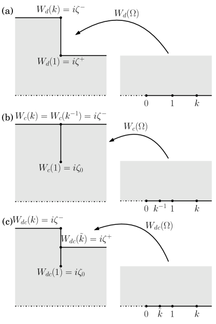
Figure 3: Transformation of the boundaries close to the discontinuity for discontinuous (a), compartmentalized (b) and discontinuous-compartmentalized (c) channels after the conformal mapping $W_{d}(\Omega)$ given by Eq. (26), $W_{c}(\Omega)$ given by Eq. (44) and $W_{dc}(\Omega)$ given by Eq. (93) respectively.

We introduce the complex variable $\tilde{z}=\tilde{x}+i\tilde{y}$, and we consider a conformal mapping

$$\tilde{z}=W_{d}(\Omega),$$ (25)

such that the channel boundary and its centerline are the images of, respectively, the positive and negative real axis (Fig. 3a) in the (complex) $\Omega$-plane. Such a mapping can be found by using the Schwarz-Christoffel method (see appendix B for details), leading to

$$W_{d}(\Omega)=\frac{\zeta^{-}}{\pi}\Bigg{\{} \frac{1}{\sqrt{k}}\operatorname{arccosh}\left[\frac{(k+1)\Omega-2k}{(k-1)\Omega}\right]$$

$$-\operatorname{arccosh}\left[\frac{2\Omega-(k+1)}{k-1}\right]\Bigg{\}}+i\zeta^{-},$$ (26)

where the parameter

$$k=(\zeta^{-}/\zeta^{+})^{2}$$ (27)

is assumed to be larger than one (without loss of generality). Note that the image of $\Omega=1$ is $W_{d}(1)=i\zeta^{+}$, the image of $\Omega=k$ is $W_{d}(k)=i\zeta^{-}$, while the image of the negative real axis is the center-line of the channel. A similar mapping has recently been usedKalinay and Percus (2010), but did not lead to explicit expressions of the effective diffusivity. We check in Appendix D that our approach is compatible with it.

Now, since $W_{d}$ is a conformal mapping, the function $\phi_{1}$ seen as a function of $\Omega_{x}=\text{Re}(\Omega),\Omega_{y}=\text{Im}(\Omega)$ must satisfy Laplace’s equation, with Neumann conditions on the boundaries which are now the positive and negative real axes. The solutions are thus of the form

$$\phi_{1}=C_{1}+C_{2}\ln|\Omega|,$$ (28)

where $C_{1}$ and $C_{2}$ are constants. These constants are determined by making explicit the relation $\tilde{x}=\mathrm{Re}\ {W_{d}(\Omega)}$ for $\tilde{x}\to-\infty$ (or, equivalently, large $\Omega$) and for $\tilde{x}\to+\infty$ (or, equivalently, small $\Omega$). We find

$$\tilde{x}\underset{|\Omega|\rightarrow+\infty}{\simeq}\frac{\zeta^{-}}{\pi}\left(\frac{1}{\sqrt{k}}\ln\frac{\sqrt{k}+1}{\sqrt{k}-1}-\ln\frac{4|\Omega|}{k-1}\right),$$ (29)

and

$$\tilde{x}\underset{|\Omega|\rightarrow 0}{\simeq}\frac{\zeta^{-}}{\pi\sqrt{k}}\left(\ln\frac{4k}{(k-1)|\Omega|}-\sqrt{k}\ln\frac{\sqrt{k}+1}{\sqrt{k}-1}\right).$$ (30)

Inserting the value of $\ln|\Omega|$ deduced from these expressions into (28) and comparing with (24) enables the identification of $C_{2}$

$$C_{2}= \frac{1}{\pi\langle\zeta^{-1}\rangle},$$ (31)

and of the jump of $F_{1}$:

$$F_{1} (0^{-})-F_{1}(0^{+})=$$

$$\frac{1}{\pi\langle\zeta^{-1}\rangle}\left(\frac{1+k}{\sqrt{k}}\ln\frac{\sqrt{k}+1}{\sqrt{k}-1}-2\ln\frac{4\sqrt{k}}{k-1}\right).$$ (32)

To summarize we have obtained an exact solution for $\phi_{1}$, seen as a function $\Omega$ instead of $\tilde{x},\tilde{y}$. We shall see in the next subsection that there is no need to know $\tilde{x}$ as a function of $\Omega$ to obtain the effective diffusivity.

II.3 Expression of the effective diffusivity for a discontinuous channel

We now use our expressions for the auxiliary function to deduce the value of the effective diffusivity. Rewriting Eq. (8) leads to

$$D_{e}=1+D_{\text{outer}}+D_{\text{inner}},$$ (33)

$$D_{\text{outer}}=\frac{1}{\langle\zeta\rangle}\int_{0}^{1}dx\zeta^{\prime}(x)f(x,R(x)),$$ (34)

$$D_{\text{inner}}=-\frac{1}{\varepsilon\langle\zeta\rangle}\int_{\varepsilon\zeta^{+}}^{\varepsilon\zeta^{-}}dyf(0,y),$$ (35)

where we have separated the contributions coming from the inner and the outer regions. The contribution of the inner region is

$$D_{\text{inner}}=-\frac{1}{\langle\zeta\rangle}\int_{\zeta^{+}}^{\zeta^{-}}d\tilde{y}[\phi_{0}+\varepsilon\phi_{1}(0,\tilde{y})].$$ (36)

However, we remark that for any harmonic function $\phi(x,y)$, we have the relation for any closed domain $V$:

$$\oint_{\partial V}dS\ n_{x}\phi=\int_{V}dV\ \nabla\phi\mathbf{e}_{x}$$

$$=-\int_{V}dV\ x\nabla^{2}\phi+\oint_{\partial V}dS\ x\mathbf{n}\cdot\nabla\phi=\oint_{\partial V}dS\ x\mathbf{n}\cdot\nabla\phi.$$ (37)

Applying this formula to $V$ large but in the boundary layer and $\phi=\phi_{0}+\varepsilon\phi_{1}$, and taking into account its boundary conditions leads to

$$D_{\text{inner}}=\frac{\zeta^{+}[F_{0}(0)+\varepsilon F_{1}(0^{+})]-\zeta^{-}[F_{0}(0)+\varepsilon F_{1}(0^{-})]}{\langle\zeta\rangle}.$$ (38)

In turn, the integral for $D_{\text{outer}}$ is dominated by the contribution coming from the outer solution (the contributions coming from the inner-solution are of higher order since $\zeta^{\prime}$ vanishes in the inner region). Hence,

$$D_{\text{outer}}=\frac{1}{\langle\zeta\rangle}\int_{0}^{1}dX\zeta^{\prime}(X)[F_{0}(X)+\varepsilon F_{1}(X)].$$ (39)

Integrating by parts, we obtain

$$D_{\text{outer}}=-\frac{1}{\langle\zeta\rangle}\int_{0}^{1}dX\zeta(X)[F_{0}^{\prime}(X)+\varepsilon F_{1}^{\prime}(X)]$$

$$+\frac{\zeta^{-}}{\langle\zeta\rangle}[F_{0}(1)+\varepsilon F_{1}(1^{-})]-\frac{\zeta^{+}}{\langle\zeta\rangle}[F_{0}(0)+\varepsilon F_{1}(0^{+})].$$ (40)

Collecting the results (38), (40) we see that

$$D_{e}=\frac{1}{\langle\zeta\rangle\langle\zeta^{-1}\rangle}\left\{1-\varepsilon\left[F_{1}(0^{-})-F_{1}(0^{+})\right]\right\},$$ (41)

which means that $D_{e}$ is simply related to the jump of the function $F_{1}$ at the discontinuity. Using Eq. (32) with $k=1/\nu^{2}$ finally leads to

$$D_{e}=\frac{1}{\langle\zeta\rangle\langle\zeta^{-1}\rangle}\left[1-\frac{\varepsilon\mu_{d}(\nu)}{\langle\zeta^{-1}\rangle}\right],$$ (42)

where $\mu_{d}$ is given by Eq. (4). This is the announced result in the case of channels presenting discontinuities. We notice that $\mu_{d}(\nu)=\mu_{d}(1/\nu)$, which is a consequence of invariance of $D_{e}$ under the transformation $x\rightarrow-x$.

II.4 Presence of several discontinuities

We now consider a channel containing several discontinuities, an example is shown in Fig. 1a. In this case we can decompose the channel into several outer regions where the equations (17) and (18) are still verified by $F_{0}^{\prime}$ and $F_{1}^{\prime}$ respectively, which means that the expressions for $F_{0}$ and $F_{1}$ are identical on all outer regions up to an additive constant.

Moreover, close to the discontinuity present at $x=x_{i}$, we see that to the leading order $F_{0}(x_{i}^{+})=F_{0}(x_{i}^{-})$, which means that $F_{0}$ is continuous in the entire channel. At the first order of perturbation, the jump $F_{1}(x_{i}^{-})-F_{1}(x_{i}^{+})$ of the function $F_{1}$ is given by Eq. (32), which depends only on the geometry of the $i^{\rm th}$ discontinuity. These conditions on $F_{0}$ and $F_{1}$ close to all singularities of the channel impose that the expressions for $F_{0}$ and $F_{1}$ do not involve any constant depending on the outer region, just a global one. Due to the relation $\int_{\partial V}dS\ n_{x}=0$, the effective diffusivity $D_{e}$ is independent of this global constant in Eq.(8). Furthermore, all discontinuities give an additive contribution to the diffusivity as can be seen from Eq.(42) at first order in $\varepsilon$. This leads to the expression (3). Let us finally note that the above only applies in the case where the discontinuities are separated by distances ${\cal O}(1)$ and when they are separated by distances ${\cal O}(\varepsilon)$ the analysis breaks down and the full inner solution with both discontinuities must be solved.

III Generalization to other types of discontinuities

III.1 Dispersion for weakly varying compartmentalized channels

We now show how to adapt the results of the previous section to consider dispersion in channels with different type of profile singularities. We consider here symmetric two-dimensional channels, which are partially obstructed by walls taken to be at the position $x=0$. We refer to these kind of channels as compartmentalized ones. At the center of these walls, we assume the presence of an opening whose (reduced) radius is $\zeta_{0}$. We denote $\zeta^{-}$ the radius just after (and before) the wall, this geometry is shown in Fig. 1b.

As in the case of a discontinuous channel, we distinguish between an inner and an outer region. In the outer region, the analysis is exactly the same, and the auxiliary function satisfies Eqs. (17) and (18). In the inner region, the function $f$ has the same structure, $\phi(\tilde{x},\tilde{y})=f(x,y)-x$ (with the same definition of the coordinates in the boundary layer). The modification of Eq. (24) for the matching condition, which gives the value of $\phi_{1}$ for large arguments is given by:

$$\phi_{1}(\tilde{x}\rightarrow\pm\infty,\tilde{y})=F_{1}(0^{\pm})-\frac{\tilde{x}}{\zeta^{-}\langle\zeta^{-1}\rangle}.$$ (43)

The function $\phi_{1}$ satisfies Laplace’s equation in the domain drawn in Fig. 3b, with Neumann conditions at the channel boundaries and at the centerline. We apply again the Schwarz-Christoffel method to find a conformal mapping enabling to solve for $\phi_{1}$. We find in Appendix B that

$$W_{c}(\Omega)= \frac{2\zeta^{-}}{\pi}\Bigg{[}\ln\left(\frac{\sqrt{k\Omega-1}+\sqrt{\Omega/k-1}}{\sqrt{(k-1/k)\Omega}}\right)-$$

$$\ln\left(\frac{\sqrt{\Omega-k}+\sqrt{\Omega-1/k}}{\sqrt{k-1/k}}\right)\Bigg{]}+i\zeta^{-},$$ (44)

where the parameter $k$ is given by

$$k=\operatorname{cotan}^{2}\frac{\pi\zeta_{0}}{4\zeta^{-}},$$ (45)

and is assumed to be larger than one. Note that $W_{c}(1/k)=W_{c}(k)=i\zeta^{-}$, $W_{c}(1)=i\zeta_{0}$ while the image of negative real axis is the centerline of the channel and the image of the positive real axis is the channel boundary (Fig. 3b). Following the same reasoning as before, we can express $\phi_{1}$ as a function of the complex variable $\Omega$, as in Eq. (28)

$$\phi_{1}=C_{1}+C_{2}\ln|\Omega|.$$ (46)

We can thus deduce the jump for $F_{1}$ from these expressions, by inverting explicitly the mapping $\tilde{x}=\mathrm{Re}\ W_{c}(\Omega)$ for $\tilde{x}\rightarrow-\infty$ (or, equivalently, $|\Omega|\rightarrow\infty$) where

$$\tilde{x}\underset{|\Omega|\rightarrow\infty}{\simeq}-\frac{\zeta^{-}}{\pi}\ln\frac{4k|\Omega|}{(k+1)^{2}},$$ (47)

and for $\tilde{x}\rightarrow+\infty$ (or, equivalently, small $|\Omega|$), for which

$$\tilde{x}\underset{|\Omega|\rightarrow 0}{\simeq}-\frac{\zeta^{-}}{\pi}\ln\frac{(k+1)^{2}|\Omega|}{4k}.$$ (48)

Comparing these expressions with Eq. (43), we identify the jump of the function $F_{1}$,

$$F_{1}(0^{-})-F_{1}(0^{+})=\frac{2}{\pi\langle\zeta^{-1}\rangle}\ln\frac{(k+1)^{2}}{4k}$$ (49)

and the value of the constant $C_{2}$

$$C_{2}=\frac{1}{\pi\langle\zeta^{-1}\rangle}.$$ (50)

We can check that Eq. (41) still holds here,

$$D_{e}=\frac{1}{\langle\zeta\rangle\langle\zeta^{-1}\rangle}\left\{1-\varepsilon\left[F_{1}(0^{-})-F_{1}(0^{+})\right]\right\},$$ (51)

so that the effective diffusivity is straightforwardly deduced from the jump of the function $F_{1}$. Setting $\nu=\zeta_{0}/\zeta^{-}$ and using the definition (45) of $k$, we finally obtain

$$D_{e}\simeq\frac{1}{\langle\zeta\rangle\langle\zeta^{-1}\rangle}\left(1-\frac{\varepsilon\mu_{c}(\nu)}{\langle\zeta^{-1}\rangle}\right),$$ (52)

which is the expression for $\mu_{c}$ given in Eq. (5) and is the announced result for dispersion in compartmentalized channels.

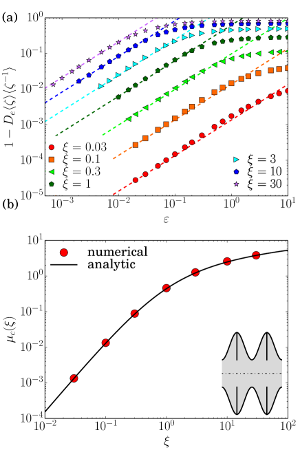
Figure 4: Numerical checks of the expression (5) for the effective diffusivity, in the case $\zeta(X\neq 0)=1+0.5\xi[1-\cos(2\pi X)]$, in the presence of a wall with reduced opening radius $\zeta_{0}=1$ at $X=0,1,...$. Here $\nu=1/(1+\xi)$. (a) $1-D_{e}/D_{\text{FJ}}$ represented for various $\xi$ [symbols: numerical solution of Eqs. (8)-(9)-(10), dashed lines: analytical prediction (3)]. (b) Full line: Value of $\mu$ predicted by (5), symbols: value of $\mu$ obtained from a linear fit of the data of (a) and assuming the behavior (3). Inset: shape of the channel. The channel shape is represented in inset for $\xi=2$.

III.2 The case of weakly varying discontinuous-compartmentalized channels

We now consider the dispersion in channels with a general type of singularity mixing the two previous cases, shown in Fig. 1c. Here, we assume that the channel is partially obstructed by walls (at $x=0,1,2...$) with a different radius between the negative (before the wall) and positive (after the wall) regions. We denote by $\zeta_{0}$ the reduced channel radius at the opening, whereas $\zeta^{-}$ is the radius just before the wall and $\zeta^{+}$ is the radius just after the wall, as shown in the left figure of Fig. 3c.

Following exactly the same steps as in the previous section, we obtain for this class of channels

$$D_{e}\simeq\frac{1}{\langle\zeta\rangle\langle\zeta^{-1}\rangle}\left(1-\frac{\varepsilon\mu_{dc}(k,\tilde{k})}{\langle\zeta^{-1}\rangle}\right),$$ (53)

Here, $\mu_{dc}$ is defined by

$$\mu_{dc}(k,\tilde{k})=\frac{1+k\tilde{k}}{\sqrt{k\tilde{k}}}\ln\frac{\sqrt{k}+\sqrt{\tilde{k}}}{\sqrt{k}-\sqrt{\tilde{k}}}-2\ln\frac{4\sqrt{k\tilde{k}}}{k-\tilde{k}},$$ (54)

and the parameters $k$ and $\tilde{k}$ are defined by the system

$$k\tilde{k} =\left(\frac{\zeta^{-}}{\zeta^{+}}\right)^{2}$$ (55)

$$\frac{\pi}{2}\left(\frac{\zeta_{0}}{\zeta^{-}}-1\right) =\frac{1}{\sqrt{k\tilde{k}}}\arctan\sqrt{\frac{\tilde{k}(k-1)}{k(1-\tilde{k})}}-\arctan\sqrt{\frac{k-1}{1-\tilde{k}}}$$ (56)

In the limit that $\nu=\zeta_{0}/\zeta^{-}\to\infty$ and fixed $\zeta_{+}/\zeta_{0}$ (i.e. when the opening is small compared to at least one radius outside the discontinuity), we obtain the following behavior

$$\mu_{dc}\simeq\begin{cases}-\frac{4}{\pi}\ln\frac{\pi\zeta_{0}}{2\sqrt{\zeta^{+}\zeta^{-}}}&(\text{if }\zeta^{+}\neq\zeta_{0})\\ \frac{2}{\pi}\left(1-\ln\frac{4\zeta^{+}}{\zeta^{-}}\right)&(\text{if }\zeta^{+}=\zeta_{0}).\end{cases}$$ (57)

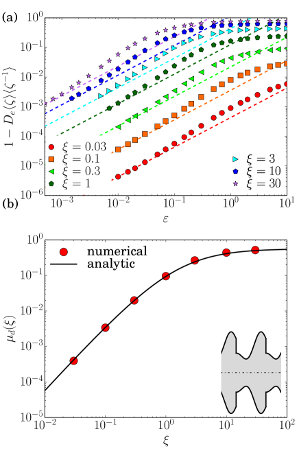
Figure 5: Numerical check of the expression (4) for the effective diffusivity of discontinuous channels, whose profile is given by $\zeta(X)=1+\xi[0.39-0.41\sin((4X+1)\pi/3)+0.20\sin((8X+1)\pi/3))]$ for $0<X<1$. Here $\nu=1/(1+\xi)$ and $\xi$ is the amplitude of variation of the channel radius. (a) $1-D_{e}/D_{\text{FJ}}$ is represented for various $\xi$ [symbols: numerical solution of Eqs. (8)-(9)-(10), dashed lines: analytical prediction (3)]. (b) Full line: Value of $\mu$ predicted by (4), symbols: value of $\mu$ obtained from a linear fit of the data of (a) and assuming the behavior (3). Inset: shape of the channel for $\xi=2$.

IV Comparison with numerical solutions and the literature

We now validate our analytical approach by comparing with the exact numerical integration of the set of partial differential equations (8)-(10). In figure 5 we show results for an example of a discontinuous channel, whose shape is represented in the inset of Fig. 5b. We first check in Fig. 5a that the first corrections to the basic Fick-Jacobs’ results are of order $\varepsilon$, as opposed to smooth channels for which the correction is of order $\varepsilon^{2}$. Furthermore, Fig. 5b shows that the coefficient of the $\varepsilon$-correction to $D_{e}$ is correctly predicted by our formula (4), thus validating our analytical approach. We perform a similar analysis for an example of channel presenting local walls defining compartments, represented in the inset of Fig. 4. The numerical analysis clearly demonstrates that the next-to-leading order term for the dispersion is correctly predicted by Eq. (5), validating our analysis for this class of channels as well.

Furthermore, the case of discontinuous channels was considered in Ref. Kalinay and Percus (2010). We check in Appendix D that our theory and that of Ref. Kalinay and Percus (2010) are consistent in the case $\zeta_{-}=2\zeta^{+}$ (which is the only case for which explicit expressions are given in Ref. Kalinay and Percus (2010)).

We can also check our analytical, asympotically-exact, result for the case of the ratchet like channel, where the profile is a periodic repetition of a linear profile $\zeta(x)=a+x$ for $x\in[0,1[$, thus presenting discontinuities at $x=0,1,2,...$. We present in Fig. 6 the exact numerical integration of the set of partial differential equations (8)-(9)-(10) compared to our first order correction to Fick-Jacobs given by Eq. (3). We also show here asymptotic results obtained by using the Kalinay and PercusKalinay and Percus (2006) formula for a position-dependent coefficient $D(x)=\arctan(R^{\prime}(x))/R^{\prime}(x)$ that is in principle exact in the linearly expanding parts of the channel. Here there are two possible procedures to apply the Lifson and Jackson formulaLifson and Jackson (1962) to determine the diffusion constant: the first where we ignore the discontinuity of the channel and find

$$\frac{D_{e}}{D_{0}}\simeq\frac{\arctan\varepsilon}{\langle\zeta\rangle\langle\zeta^{-1}\rangle\varepsilon},$$ (58)

which gives a correction to Fick-Jacobs result of order $\varepsilon^{2}$ and is thus clearly incompatible with our exact results (see Fig. 6). Secondly the vertical line at the end of the channel between $y=1+a$ and $y=a$ can be replaced by a straight line of finite slope between $(1-\delta,1+a)$ and $(1,a)$, applying the Lifson-Jackson formula and then taking the limit $\delta\to 0$. Following this procedure leads to Mangeat, Guérin, and Dean (2017a)

$$\frac{D_{e}}{D_{0}}=\frac{1}{\langle\zeta\rangle\langle\zeta^{-1}\rangle\left(\frac{2}{\pi}\varepsilon+\frac{\varepsilon}{\arctan\varepsilon}\right)}.$$ (59)

Interestingly, this result includes a correction of order $\varepsilon$, but with a prefactor that disagrees with the exact result Eq. (3). This is not surprising since the arctangent formula for $D(x)$ is obtained by neglecting all high-order derivatives of $R(x)$ in the expansion series, whereas such terms are infinite at the discontinuity. Hence, our approach provides more precise results for this kind of channels, even if it does not include the effect of higher order terms in the $\varepsilon$ expansion.

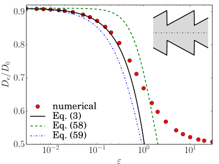
Figure 6: Effective diffusivity of the ratchet channel $\zeta(x)=0.25+x$. The dots correspond to the numerical solution of the partial differential equations Eqs. (8)-(9)-(10), the straight line represents the first order correction to FJ given by Eqs. (3)-(4). We also show results obtained by using the partially resumed formula for $D(x)$ given in Ref. Kalinay and Percus (2006) (dashed line: Eq.(58), dash-dotted line: Eq. (59), see text).

V Effective trapping rates

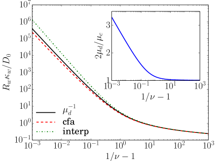
Figure 7: Trapping rate $\kappa_{w}R_{w}/D_{0}$ as a function of $\nu=R_{n}/R_{w}$. Our theory (continuous black line) is compared to expressions for trapping rates proposed in Ref.Berezhkovskii et al. (2006), obtained by the constant flux approximation [CFA, Eq. (67), dashed red line] or interpolation [interp, Eq. (68), green dotted line]. In inset, we compare the ratio of trapping rates for the discontinuities and for compartmentalized channels, which is found to differ from unity.

A widely used approach to deal with discontinuous channels is the use of the boundary homogenization methodBerezhkovskii, Barzykin, and Zitserman (2009); Makhnovskii, Berezhkovskii, and Zitserman (2010); Antipov et al. (2014); Makhnovskii, Berezhkovskii, and Zitserman (2009); Antipov et al. (2013). In this class of approaches, one assumes that one can define a one dimensional stochastic dynamics for $x(t)$, with associated probability density function $p(x,t)$ that satisfies a diffusion equation in the smooth part of the channel. The presence of discontinuities is taken into account by introducing trapping rates $\kappa^{\pm}$ in the flux continuity equation

$$-D_{0}\partial_{x}p|_{x=0^{+}}=-D_{0}\partial_{x}p|_{x=0^{-}}=\kappa^{-}p_{x=0^{-}}-\kappa^{+}p_{x=0^{+}}.$$ (60)

Roughly speaking, $\kappa^{-}$ quantifies the likelihood, for a particle on one side of the discontinuity, to cross it (and thus be re-injected on the other side of it). The ratio of trapping rates can be deduced from detailed balance (here in the two-dimensional case)

$$\frac{\kappa^{+}}{\kappa^{-}}=\frac{\zeta^{-}}{\zeta^{+}}.$$ (61)

Here we show that our approach is compatible with the concept of trapping rates, and that it provides a means to determine them exactly in the limit $\varepsilon\to 0$. Consider first the case of a channel formed by wide ($w$) and narrow ($n$) portions of constant radius $R_{w},R_{n}$ and length $l_{w},l_{n}$, with $L=l_{n}+l_{w}$. One introduces two kinds of trapping rates: $\kappa_{w}$ quantifying the transitions from the wide to the narrow portions, and conversely $\kappa_{n}$ that quantifies the transitions from the narrow to the wide portions. The effective diffusivity in such channels reads (see Eq. (31) of Ref. Makhnovskii, Berezhkovskii, and Zitserman (2010))

$$D_{e}=\frac{D_{0}L^{2}}{l_{n}^{2}+l_{w}^{2}+l_{n}l_{w}\left(\frac{\kappa_{w}}{\kappa_{n}}+\frac{\kappa_{n}}{\kappa_{w}}\right)+2D_{0}\left(\frac{l_{n}}{\kappa_{n}}+\frac{l_{w}}{\kappa_{w}}\right)}.$$ (62)

Using the detailed balance condition (61), we find that the above formula simplifies to

$$D_{e}=\frac{D_{0}}{\langle R\rangle\langle R^{-1}\rangle+\frac{2D_{0}}{R_{w}\kappa_{w}L}\langle R\rangle},$$ (63)

and in the weakly varying limit we obtain

$$D_{e}\simeq\frac{D_{0}}{\langle R\rangle\langle R^{-1}\rangle}\left(1-\frac{2D_{0}}{R_{w}\kappa_{w}\langle R^{-1}\rangle L}+\mathcal{O}(\varepsilon^{2})\right).$$ (64)

For the same channel, our approach leads to

$$D_{e}\simeq\frac{D_{0}}{\langle R\rangle\langle R^{-1}\rangle}\left(1-2\frac{\mu_{d}}{L\langle R^{-1}\rangle}+\mathcal{O}(\varepsilon^{2})\right).$$ (65)

where the factor $2$ comes from the fact that they are two discontinuities per channel period. Comparing the above formulas gives

$$\frac{R_{w}\kappa_{w}}{D_{0}}=\frac{R_{n}\kappa_{n}}{D_{0}}=\frac{1}{\mu_{d}}.$$ (66)

The above formula suggests that asymptotically exact results for the trapping rates are obtained from our analysis.

In the boundary homogenization method, trapping rates are usually determined by considering the flux of particles on a surface presenting sticky patches. Although in most cases this method is applied to the three dimensional case, it is interesting to test its validity in the present two-dimensional situation. The corresponding problem is that of particles diffusing to a surface presenting straight strips. Two different approximate formulasBerezhkovskii et al. (2006) were proposed for the trapping rate, the first one in the constant flux approximation (CFA) leads to

$$\frac{R_{w}\kappa_{w}^{\text{(cfa)}}}{D_{0}}\simeq\frac{1}{2\nu}\frac{\pi^{3}\nu^{3}}{\sum_{n=1}^{\infty}(1/n^{3})\sin^{2}(\pi n\nu)},$$ (67)

where $\nu=R_{n}/R_{w}$. In Ref. Berezhkovskii et al. (2006), another (interpolation) formula is proposed

$$\frac{R_{w}\kappa_{w}^{\text{(interp)}}}{D_{0}}\simeq\frac{\pi}{2(1-\nu)^{2}\ln(2.6+0.7/\nu)}.$$ (68)

It is interesting to compare these approximate values of the trapping rates with our exact calculation. We see on Fig. 7 that the three formulas give similar values for $\kappa_{w}$. For $\nu\to 0$, all expressions of $\kappa_{w}$ have the same dominant behavior $1/\ln\nu$, given by Eq. (57) for our exact value. They however differ for finite values of $\nu$, which is quantified by our approach.

Next, in the case of channels made of a periodic arrangement of compartments of constant radius $R_{w}$ and length $L$, separated by infinitely thin walls, with openings of radius $R_{n}$, we call $\kappa_{c}$ the trapping rate (which is usually called the permeability $P$), and the effective diffusivity readsMakhnovskii, Berezhkovskii, and Zitserman (2009)

$$D_{e}=\frac{D_{0}}{1+D_{0}/(\kappa_{c}L)}\simeq D_{0}\left(1-\frac{D_{0}}{\kappa_{c}L}\right),$$ (69)

which leads to

$$\frac{\kappa_{c}R_{w}}{D_{0}}=\frac{1}{\mu_{c}}.$$ (70)

In the literatureMakhnovskii, Berezhkovskii, and Zitserman (2009) it is suggested that $\kappa_{c}\simeq\kappa_{w}/2$, since a particle that is exactly between the two compartments can switch with equal probability on each side. However, our theory clearly shows that such an argument is only an approximation: on the inset of Fig. 7, we see that the exact ratio of $2\kappa_{c}/\kappa_{d}$, which in our theory is given by $2\mu_{d}/\mu_{c}$, is clearly different from unity.

VI Conclusion

Let us now summarize our findings. We have calculated the effective diffusivity of non-interacting tracer particles diffusing in symmetric channels of non-uniform radius presenting singularities. In such channels, the usual Fick-Jacobs’ (FJ) approach is valid at lowest order only and provides only a rough approximation of the diffusion coefficient. This is in contrast to smooth channels, where the FJ theory can be systematically improved by taking into account higher order terms of the parameter $\varepsilon$, which measures the ratio of equilibration time in the lateral and axial directions. Here, we have identified the next-to-leading order term for the Fick-Jacobs’ approach in two-dimensional discontinuous channels. We found that each discontinuity gives rise to an additive negative correction to the diffusion constant. This is compatible with modeling of discontinuities in terms of localized trapping rates. Our theory enables us to identify exact expressions of these trapping rates (by requiring that their use leads to asymptotically to the exact expressions of the diffusivity obtained here). The approach here provides explicit expressions for these trapping rates in terms of the geometrical parameters of the discontinuity. Here we have considered two types of discontinuities: (i) the case of an abrupt change of radius, and (ii) the presence of thin walls with small opening that separate the channel into compartments. Our formalism could however be used to explore dispersion properties for other singularities, and can also be extended to the case of three dimensional channels. Our results help in precisely quantifying the concepts of kinetic entropic barriers associated with profile singularities.

Appendix A Calculation of the functions $F_{i}$

Here we describe how to calculate the functions $F_{0},F_{1},...$ appearing in the expansion (16). At order $\varepsilon^{0}$ and $\varepsilon^{1}$, Eq. (14) becomes

$$\partial_{Y}^{2}F_{0}=\partial_{Y}^{2}F_{1}=0$$ (71)

in the bulk, and the boundary conditions read

$$\partial_{Y}F_{0}|_{Y=\zeta(X)}=\partial_{Y}F_{1}|_{Y=\zeta(X)}=0,$$ (72)

$$\partial_{Y}F_{0}|_{Y=0}=\partial_{Y}F_{1}|_{Y=0}=0.$$ (73)

We thus deduce that the functions $F_{0}$ and $F_{1}$ do not depend on $Y$, and we denote them by $F_{0}(X)$ and $F_{1}(X)$. Examining the ${\cal O}(\varepsilon^{2})$ terms in (14) yields

$$\partial_{Y}^{2}F_{2}(X,Y)+F_{0}^{\prime\prime}(X)=0.$$ (74)

Integrating this equation with respect to $Y$, and using $\partial_{Y}F_{2}|_{Y=0}=0$ yields

$$\partial_{Y}F_{2}(X,Y)=-F_{0}^{\prime\prime}(X)Y.$$ (75)

Now, expanding Eq. (15) at order $\varepsilon^{2}$ enables us to identify the boundary condition for $F_{2}$ as

$$\partial_{Y}F_{2}|_{Y=\zeta(X)}=\zeta^{\prime}(X)[F_{0}^{\prime}(X)-1],$$ (76)

which can be inserted into Eq. (75), yielding

$$\zeta^{\prime}(X)[F_{0}^{\prime}(X)-1]=-F_{0}^{\prime\prime}(X)\zeta(X).$$ (77)

The solutions to this equation are of the form

$$F_{0}^{\prime}(X)=1-\frac{\lambda_{0}}{\zeta(X)},$$ (78)

where $\lambda_{0}$ is, so far, an undetermined constant. We can proceed further by anticipating here that $F_{0}$ is a continuous function at $X=0$ (modulo 1). Such property can be justified by considering the matching condition with the solution in the inner region (see the next section), and it is also justified since we do not expect that the discontinuity of the profile modifies the leading order term of the FJ approximation. With this assumption, the periodicity implies that $\lambda_{0}=\langle\zeta^{-1}\rangle^{-1}$ and thus

$$F_{0}^{\prime}(X)=1-\frac{1}{\langle\zeta^{-1}\rangle\zeta(X)}.$$ (79)

which is Eq. (17).

Now, expanding at order $\varepsilon^{3}$ the equations for $F$ yields

$$\partial_{Y}^{2}F_{3}+F_{1}^{\prime\prime}(X)=0,$$ (80)

$$\partial_{Y}F_{3}|_{Y=\zeta(X)}=\zeta^{\prime}(X)F_{1}^{\prime}(X).$$ (81)

Integrating Eq. (80) and using $\partial_{Y}F_{3}|_{Y=0}=0$ yields $\partial_{Y}F_{3}(X,Y)=-F_{1}^{\prime\prime}(X)Y$, comparing to Eq. (81) we obtain

$$\zeta^{\prime}(X)F_{1}^{\prime}(X)=-F_{1}^{\prime\prime}(X)\zeta(X).$$ (82)

The solutions of this equation are of the form

$$F_{1}^{\prime}(X)=\frac{\lambda_{1}}{\zeta(X)}.$$ (83)

where $\lambda_{1}$ is a constant. Note that $\lambda_{1}$ is related to the difference of the values on each side of the profile discontinuity by

$$\lambda_{1}=\frac{F_{1}(1^{-})-F_{1}(0^{+})}{\langle\zeta^{-1}\rangle}=\frac{F_{1}(0^{-})-F_{1}(0^{+})}{\langle\zeta^{-1}\rangle},$$ (84)

where we have used the periodicity of $F$ in the second equality. $F_{1}^{\prime}$ is thus given by

$$F_{1}^{\prime}(X)=\frac{F_{1}(0^{-})-F_{1}(0^{+})}{\langle\zeta^{-1}\rangle\zeta(X)}.$$ (85)

which is exactly Eq. (18).

Appendix B Details on conformal maps

According to the rules of the Schwarz Christoffel mappingMathews and Howell (2012), the complex derivative of the mapping $\tilde{x}=W_{d}(\Omega)$ in the case of a discontinuous channel (Fig. 3a) is of the form

$$W_{d}^{\prime}(\Omega)=K_{0}\frac{\sqrt{\Omega-1}}{\Omega\sqrt{\Omega-k}},$$ (86)

where $K_{0}$ and $k$ are constants to be determined below. Integrating the above expression yields

$$W_{d}(\Omega)= K_{0}\Bigg{\{}\operatorname{arccosh}\left[\frac{2\Omega-(k+1)}{k-1}\right]$$

$$-\frac{1}{\sqrt{k}}\operatorname{arccosh}\left[\frac{(k+1)\Omega-2k}{(k-1)\Omega}\right]\Bigg{\}}+K_{1}.$$ (87)

The conditions that $W_{d}(1)=i\zeta^{+}$, $W_{d}(k)=i\zeta^{-}$ and $\mathrm{Im}\ W_{d}(0^{-})=0$ then fix the values of $k,\ K_{0}$ and $K_{1}$, and we find

$$\sqrt{k}=\frac{\zeta^{-}}{\zeta^{+}},K_{1}=i\zeta^{-},\ K_{0}=-\frac{\zeta^{-}}{\pi}.$$ (88)

In the case of compartmentalized channels (Fig. 3b), we look for a mapping of the form

$$W_{c}^{\prime}(\Omega)=K_{0}\frac{\Omega-1}{\Omega\sqrt{(\Omega-k)(\Omega-\tilde{k})}}.$$ (89)

Integrating leads to

$$W_{c}(\Omega)= -2K_{0}\Bigg{[}\frac{1}{\sqrt{k\tilde{k}}}\ln\left(\frac{\sqrt{k(\Omega-\tilde{k})}+\sqrt{\tilde{k}(\Omega-k)}}{\sqrt{(k-\tilde{k})\Omega}}\right)$$

$$-\ln\left(\sqrt{\Omega-k}+\sqrt{\Omega-\tilde{k}}\right)\Bigg{]}+K_{1}.$$ (90)

The conditions $W_{c}(1)=i\zeta_{0}$, $W_{c}(k)=W_{c}(\tilde{k})=i\zeta^{-}$ and $\mathrm{Im}\ W_{c}(0^{-})=0$ then determine the values of $k,\ \tilde{k},\ K_{0}$ and $K_{1}$; we find

$$k=\frac{1}{\tilde{k}}=\operatorname{cotan}^{2}\frac{\pi\zeta_{0}}{4\zeta^{-}},\ K_{0}=-\frac{\zeta^{-}}{\pi},$$ (91)

$$K_{1}=i\zeta^{-}+\frac{\zeta^{-}}{\pi}\ln(k-1/k).$$ (92)

Appendix C Calculations for weakly varying discontinuous-compartmentalized channels

Here we describe the calculations leading to the result (54), for channels partially obstructed by walls at a given position $x=0$ and with a discontinuity of the radius between the negative (before the wall) and positive (after the wall) regions. The notations are those of Fig. 3c. As in the case of a discontinuous channel, we distinguish between an inner and an outer region. In the outer region, the analysis is exactly the same, and the auxiliary function satisfies Eqs. (17) and (18). In the inner region, the function $f$ has the same structure, $\phi(\tilde{x},\tilde{y})=f(x,y)-x$ (with the same definition of the coordinates in the boundary layer). The matching condition given by Eq. (24) is still satisfied.

The function $\phi_{1}$ satisfies Laplace’s equation in the domain drawn in Fig. 3c, with Neumann conditions at the channel boundaries and at the centerline. We apply again the Schwarz-Christoffel method to find a conformal mapping enabling to solve for $\phi_{1}$. We find from the expression (90) that

$$W_{dc}(\Omega)= \frac{2\zeta^{-}}{\pi}\Bigg{[}\frac{1}{\sqrt{k\tilde{k}}}\ln\left(\frac{\sqrt{k(\Omega-\tilde{k})}+\sqrt{\tilde{k}(\Omega-k)}}{\sqrt{(k-\tilde{k})\Omega}}\right)$$

$$-\ln\left(\frac{\sqrt{\Omega-k}+\sqrt{\Omega-\tilde{k}}}{\sqrt{k-\tilde{k}}}\right)\Bigg{]}+i\zeta^{-},$$ (93)

Here, the parameters $k$ and $\tilde{k}$ are chosen such that $W_{dc}(\tilde{k})=i\zeta^{+}$, $W_{dc}(k)=i\zeta^{-}$, $W_{dc}(1)=i\zeta_{0}$ while the image of negative real axis is the centerline of the channel and the image of the positive real axis is the channel boundary (Fig. 3c). This leads to the system

$$k\tilde{k} =\left(\frac{\zeta^{-}}{\zeta^{+}}\right)^{2},$$ (94)

$$\frac{\pi}{2}\left(\frac{\zeta_{0}}{\zeta^{-}}-1\right) =\frac{1}{\sqrt{k\tilde{k}}}\arctan\sqrt{\frac{\tilde{k}(k-1)}{k(1-\tilde{k})}}-\arctan\sqrt{\frac{k-1}{1-\tilde{k}}}.$$ (95)

Following the same reasoning as before, we can express $\phi_{1}$ as a function of the complex variable $\Omega$, following the Eq. (28). We can thus deduce the jump for $F_{1}$ from these expressions, by inverting explicitly the mapping $\tilde{x}=\mathrm{Re}\ W_{dc}(\Omega)$ for $\tilde{x}\rightarrow-\infty$ (or, equivalently, $|\Omega|\rightarrow\infty$) where

$$\tilde{x}\underset{|\Omega|\rightarrow\infty}{\simeq}\frac{\zeta^{-}}{\pi}\left[\frac{1}{\sqrt{k\tilde{k}}}\ln\frac{\sqrt{k}+\sqrt{\tilde{k}}}{\sqrt{k}-\sqrt{\tilde{k}}}-\ln\frac{4|\Omega|}{k-\tilde{k}}\right],$$ (96)

and for $\tilde{x}\rightarrow+\infty$ (or, equivalently, small $|\Omega|$), for which

$$\tilde{x}\underset{|\Omega|\rightarrow 0}{\simeq}\frac{\zeta^{-}}{\pi}\left[\frac{1}{\sqrt{k\tilde{k}}}\ln\frac{4k\tilde{k}}{(k-\tilde{k})\Omega}-\ln\frac{\sqrt{k}+\sqrt{\tilde{k}}}{\sqrt{k}-\sqrt{\tilde{k}}}\right].$$ (97)

Comparing these expressions with Eq. (24) we identify the jump of the function $F_{1}$,

$$F_{1} (0^{-})-F_{1}(0^{+})=$$

$$\frac{1}{\pi\langle\zeta^{-1}\rangle}\left[\frac{1+k\tilde{k}}{\sqrt{k\tilde{k}}}\ln\frac{\sqrt{k}+\sqrt{\tilde{k}}}{\sqrt{k}-\sqrt{\tilde{k}}}-2\ln\frac{4\sqrt{k\tilde{k}}}{k-\tilde{k}}\right].$$ (98)

We can check that Eq. (41) still holds here, and we finally obtain Eq.(54).

Appendix D Comparison with the Kalinay Percus approach

Here we control that our approach is consistent with the results of Kalinay and PercusKalinay and Percus (2010), who mapped the dynamics of $x(t)$ on a one-dimensional diffusive dynamics, whose diffusion coefficient at the vicinity of a discontinuity at $x=0$ reads

$$\frac{D_{0}}{D(x)}=R(x)\frac{d}{dx}\frac{x+C_{t}\Theta(x)+C_{0}}{R(x)}$$ (99)

where $C_{t}$ and $C_{0}$ depend on $\zeta^{\pm}$. Let us recall here the Lifson-JacksonLifson and Jackson (1962) formula which provides the effective diffusivity for one-dimensional particles with diffusion coefficient $D(x)$ moving in two-dimensional channels:

$$D_{e}=\frac{1}{\langle R\rangle\langle[D(x)R(x)]^{-1}\rangle}.$$ (100)

If we insert (99) into the above expression, we see that for a periodic channel, made of flat portions with radii $R_{w}$ and $R_{n}$ for respectively wide and narrow regions (as in Sec. V), we obtain

$$D_{e}=\frac{D_{0}}{\langle R\rangle\langle R^{-1}\rangle+2\left(\frac{C_{t}+C_{0}}{R_{n}}-\frac{C_{0}}{R_{w}}\right)\langle R\rangle}.$$ (101)

This formula is compatible with Eq. (63) for an inverse trapping rate equal to

$$\frac{D_{0}}{R_{w}\kappa_{w}}=\frac{C_{t}+C_{0}}{R_{n}}-\frac{C_{0}}{R_{w}}.$$ (102)

From the Eq. (66), we can thus identify

$$\mu_{d}\left(\frac{R_{n}}{R_{w}}\right)=\left(\frac{C_{t}+C_{0}}{R_{n}}-\frac{C_{0}}{R_{w}}\right).$$ (103)

The values of $C_{t}$ and $C_{0}$ are given by Kalinay and PercusKalinay and Percus (2010) for the radii $R_{n}=\pi/2$ and $R_{w}=\pi$, yielding $C_{t}=1.21640$ and $C_{0}=-1.64792$. This leads to the value of the inverse of trapping rate $D_{0}/(R_{w}\kappa_{w})\simeq 0.2498$. For $\nu=R_{n}/R_{w}=0.5$, our approach gives $D_{0}/(R_{w}\kappa_{w})=\mu_{d}(\nu=0.5)\simeq 0.2498$. Our result is thus compatible with that of Kalinay and PercusKalinay and Percus (2010) for $\nu=0.5$.

References

- Le Borgne, Dentz, and Villermaux (2013) T. Le Borgne, M. Dentz, and E. Villermaux, Phys. Rev. Lett. 110, 204501 (2013).
- Dentz et al. (2011) M. Dentz, T. Le Borgne, A. Englert, and B. Bijeljic, J. Contam. Hydrol. 120, 1 (2011).
- Barros et al. (2012) F. P. Barros, M. Dentz, J. Koch, and W. Nowak, Geophys. Res. Lett. 39 (2012).
- Bernate and Drazer (2012) J. A. Bernate and G. Drazer, Phys. Rev. Lett. 108, 214501 (2012).
- Brusseau (1994) M. L. Brusseau, Rev. Geophys. 32, 285 (1994).
- Dean et al. (2007) D.S. Dean, I.T. Drummond, and R.R. Horgan, J. Stat. Mech , P07013 (2007).
- Condamin et al. (2007) S. Condamin, O. Bénichou, V. Tejedor, R. Voituriez, and J. Klafter, Nature 450, 77 (2007).
- Burada et al. (2009) P. S. Burada, P. Hänggi, F. Marchesoni, G. Schmid, and P. Talkner, ChemPhysChem 10, 45 (2009).
- Malgaretti, Pagonabarraga, and Rubi (2013) P. Malgaretti, I. Pagonabarraga, and M. Rubi, Frontiers in Physics 1, 21 (2013).
- Bressloff and Newby (2013) P. C. Bressloff and J. M. Newby, Rev. Mod. Phys. 85, 135 (2013).
- Holcman and Schuss (2013) D. Holcman and Z. Schuss, Rep. Progr. Phys. 76, 074601 (2013).
- Yang et al. (2017) X. Yang, C. Liu, Y. Li, F. Marchesoni, P. Hänggi, and H. Zhang, Proc. Natl. Acad. Sci. U. S. A. , 201707815 (2017).
- Burada et al. (2008) P. S. Burada, G. Schmid, P. Talkner, P. Hänggi, D. Reguera, and J. M. Rubi, BioSystems 93, 16 (2008).
- Reguera et al. (2006) D. Reguera, G. Schmid, P. S. Burada, J. M. Rubi, P. Reimann, and P. Hänggi, Phys. Rev. Lett. 96, 130603 (2006).
- Kalinay and Percus (2006) P. Kalinay and J. Percus, Phys. Rev. E 74, 041203 (2006).
- Malgaretti, Pagonabarraga, and Miguel Rubi (2016) P. Malgaretti, I. Pagonabarraga, and J. Miguel Rubi, J. Chem. Phys. 144, 034901 (2016).
- Jacobs (1967) M. Jacobs, Diffusion processes (Springer, New-York, 1967).
- Lifson and Jackson (1962) S. Lifson and J. L. Jackson, J. Chem. Phys. 36, 2410 (1962).
- Note (1) Note that Ref.Kalinay and Percus (2006) uses as the small parameter, where and are, respectively, the local diffusion coefficients in the lateral and longitudinal directions. Expansions in this parameter or in powers of are equivalent. Note also that our parameter is proportional to used in Ref.Dorfman and Yariv (2014).
- Zwanzig (1992) R. Zwanzig, J Phys. Chem. 96, 3926 (1992).
- Reguera and Rubi (2001) D. Reguera and J. Rubi, Phys. Rev. E 64, 061106 (2001).
- Kalinay and Percus (2005a) P. Kalinay and J. Percus, Phys. Rev. E 72, 061203 (2005a).
- Kalinay and Percus (2005b) P. Kalinay and J. Percus, J. Chem. Phys. 122, 204701 (2005b).
- Kalinay and Percus (2010) P. Kalinay and J. K. Percus, Phys. Rev. E 82, 031143 (2010).
- Martens et al. (2011) S. Martens, G. Schmid, L. Schimansky-Geier, and P. Hänggi, Phys. Rev. E 83, 051135 (2011).
- Bradley (2009) R. M. Bradley, Phys. Rev. E 80, 061142 (2009).
- Berezhkovskii and Szabo (2011) A. Berezhkovskii and A. Szabo, J. Chem. Phys. 135, 074108 (2011).
- Dagdug and Pineda (2012) L. Dagdug and I. Pineda, J. Chem. Phys. 137, 024107 (2012).
- Valdes and Guzman (2014) C. V. Valdes and R. H. Guzman, Phys. Rev. E 90, 052141 (2014).
- Dorfman and Yariv (2014) K. D. Dorfman and E. Yariv, J. Chem. Phys. 141, 044118 (2014).
- Mangeat, Guérin, and Dean (2017a) M. Mangeat, T. Guérin, and D. S. Dean, J. Stat. Mech. Theory Exp , 123205 (2017a).
- Berezhkovskii, Barzykin, and Zitserman (2009) A. M. Berezhkovskii, A. V. Barzykin, and V. Y. Zitserman, J. Chem. Phys. 131, 224110 (2009).
- Antipov et al. (2013) A. E. Antipov, A. V. Barzykin, A. M. Berezhkovskii, Y. A. Makhnovskii, V. Y. Zitserman, and S. M. Aldoshin, Phys. Rev. E 88, 054101 (2013).
- Marchesoni (2010) F. Marchesoni, J. Chem. Phys. 132, 166101 (2010).
- Borromeo and Marchesoni (2010) M. Borromeo and F. Marchesoni, Chem. Phys. 375, 536 (2010).
- Mangeat, Guérin, and Dean (2017b) M. Mangeat, T. Guérin, and D. S. Dean, Europhys. Lett. 118, 40004 (2017b).
- Guérin and Dean (2015a) T. Guérin and D. S. Dean, Phys. Rev. Lett. 115, 020601 (2015a).
- Guérin and Dean (2015b) T. Guérin and D. S. Dean, Phys. Rev. E 92, 062103 (2015b).
- Brenner and Edwards (1993) H. Brenner and D. A. Edwards, Macrotransport theory (Butterworth-Heinemann, Boston, 1993).
- Berezhkovskii et al. (2006) A. M. Berezhkovskii, M. I. Monine, C. B. Muratov, and S. Y. Shvartsman, J. Chem. Phys. 124, 036103 (2006).
- Makhnovskii, Berezhkovskii, and Zitserman (2010) Y. A. Makhnovskii, A. Berezhkovskii, and V. Y. Zitserman, Chem. Phys. 367, 110 (2010).
- Antipov et al. (2014) A. Antipov, Y. A. Makhnovskii, V. Y. Zitserman, and S. Aldoshin, Russ. J. Phys. Chem. B 8, 752 (2014).
- Makhnovskii, Berezhkovskii, and Zitserman (2009) Y. A. Makhnovskii, A. Berezhkovskii, and V. Y. Zitserman, J. Chem. Phys. 131, 104705 (2009).
- Mathews and Howell (2012) J. H. Mathews and R. W. Howell, Complex analysis for mathematics and engineering (Jones & Bartlett Publishers, 2012).