1 Introduction

Coronal Mass Ejections (CMEs) are the most energetic events in our solar system. They are large structures of plasma confined in a sheared/twisted magnetic field being ejected from the low solar corona. Generally, they originate from the magnetically active regions of the Sun. With ejected mass reaching $10^{12}$ kg and speeds up to 3000 km/s, they carry a huge amount of kinetic and magnetic energy [Chen, 2011]. A CME directed towards Earth can cause extreme space weather conditions that affect space-borne and ground-based technological systems. Therefore, predicting the CME eruption, its arrival time at Earth, and possible impact on it are of great importance to our technologically-advanced society. Many past and present observatories and instruments (both space-borne and ground-based) have helped us understand the Sun–Earth connection. A number of CME arrival time models have been proposed over the years. They include empirical models [e.g. Vandas et al., 1996, Brueckner et al., 1998, Gopalswamy et al., 2005, Wang et al., 2002, Manoharan et al., 2004], drag based models used to predict CME arrival times [Vrsnak, 2001, Vrsnak & Gopalswamy, 2002], and such physics based-models such as, e.g., Shock Time of Arrival (STOA), STOA-2 [Moon, 2002].

Substantial success has been achieved in numerical modeling of CMEs [e.g. Amari et al., 2011, 2014, Antiochos et al., 1999, Aulanier et al., 2010, Roussev et al., 2012, Jiang et al., 2016, Forbes et al., 2006, Mikic & Linker, 1994, Moore et al., 2001, Schmieder et al., 2015, Torok & Kliem, 2005, Kliem & Torok, 2006, Gibson & Low, 1998, Titov & Demoulin, 1999, Titov et al., 2014, Linker & Mikic, 1995, Chane et al., 2005, Chen, 2011, Jacobs et al., 2006, Jin et al., 2017a, Lugaz et al., 2017, Torok et al., 2004, Fan & Gibson, 2007, Forbes & Priest, 1995, Lin & Forbes, 2000, Hu, 2001] and their propagation into the inner heliosphere [e.g. Detman et al., 2011, van der Holst et al., 2014, Feng et al., 2011, 2015, Hayashi, 2013, Intriligator et al., 2012, Lee et al., 2014, Leake et al., 2014, Linker et al., 2016, Lionello et al., 2009, 2016, Lugaz & Roussev, 2011, Manchester et al., 2006, Merkin et al., 2016, Odstrcil & Pizzo, 1999a, 2009, Oran et al., 2015, Riley et al., 2003, 2015a, 2015b, Riley & Richardson, 2013, Roussev et al., 2003b, Sokolov et al., 2013, Usmanov & Goldstein, 2006, Usmanov et al., 2011, Wang et al., 2011, Wu et al., 2009].

Previous CME models such as the blob model and over-pressured spherical plasmoid [e.g. Chane et al., 2005, Odstrcil & Pizzo, 1999a] do not take into consideration the magnetic field inside a CME. These approaches do not give us a complete picture of CME propagation because the conversion from magnetic to kinetic energy is an integral part of this phenomenon. Processes like CME-CME collisions in the interplanetary space rely heavily on the CME magnetic field. Thus, the above models fail to simulate the full complexity of CME events [Shen et al., 2017]. The magnetic field produced by a CME is one of the critical parameters determining its geoeffectiveness, i.e., the ability to disturb Earth’s magnetosphere and upper atmosphere. CMEs with a negative z-component of the magnetic field vector, $B_{z}$, have been observed to be more geoeffective due to coupling with the positive $B_{z}$ of Earth’s magnetosphere, where the z-axis is perpendicular to the solar ecliptic plane [Lockwood et al., 2016]. Thus, CME models, that ignore such magnetic structure can hardly be used to predict their geoeffectiveness.

In this paper, we use a Gibson–Low (GL) type flux rope model [Gibson & Low, 1998] to simulate a CME. Similar models have previously been applied by, e.g.,  Manchester et al. [2004a, b, 2006, 2014a, 2014b], Jin et al. [2016, 2017a, 2017b], Kataoka et al. [2009], Lugaz et al. [2005, 2007], Poedts & Pomoell [2017], Pomoell et al. [2017], Shiota & Kataoka [2016]. Jin et al. [2017b] describe a data-constrained CME model to find the GL flux rope parameters from observations. They use the size of neutral line in the source active region to find the GL size parameters. The GL magnetic field strength is found indirectly from a parametric study.

In the present paper, we acquire the GL flux rope size parameters directly from coronagraph observations of a CME by using the Graduated Cylindrical Shell (GCS) method [Thernisien et al., 2006]. Afterwards, a parametric study is performed to compute the magnetic field strength of flux rope indirectly. This method is described in detail in section 2.

This approach is complementary to the CME model of Jin et al. [2017b]. It allows us to determine the initial flux rope geometry more accurately because we do not impose excessive energy in the initial flux rope configuration thereby avoiding its excessive heating and acceleration. Moreover, our method of determining the GL flux rope parameters from the observational data can be automatized by a user friendly GUI similar to the Eruptive Event Generator (Gibson and Low)(EEGGL) [Borovikov et al., 2017] in the Community Coordinated Modeling Center (CCMC). While complex CME models involving an energy buildup before eruption [e.g. Titov & Demoulin, 1999, Amari et al., 2014] exist, our model implements a rather simple, but data driven, eruption mechanism triggered by the force imbalance between the initial flux rope and the surrounding background solar wind as soon as the flux rope is inserted. As compared with a number of CME initiation models described in the reviews of  Chen [2011] and  Aulanier [2013], especially taking into account existing limitations on data-driven models, our approach is computationally more efficient and provides a practical alternative for operational space weather forecasting.

We have implemented this CME model as a module in the Multi-Scale Fluid-Kinetic Simulation Suite (MS-FLUKSS) [Pogorelov et al., 2014]– a suite of adaptive mesh refinement (AMR) codes designed to solve the coupled system of magnetohydrodynamics (MHD), gas dynamics Euler, and kinetic Boltzmann equations [Borovikov et al., 2009, 2013, Pogorelov et al., 2009, 2013]. MS-FLUKSS is built upon the Chombo AMR framework [Colella et al., 2007]. It also has modules that treat pickup ions either kinetically or as a separate fluid, and turbulence models applicable beyond the Alfvénic surface [Gamayunov et al., 2012, Kryukov et al., 2012, Adhikari et al., 2015].

Previously, we have studied a number of CME events generated by the blob model [Chane et al., 2005] in the inner heliosphere using MS-FLUKSS [Pogorelov et al., 2017]. Our present CME model employs a newly developed data-driven MHD global solar corona model [Yalim et al., 2017].

The structure of the paper is as follows. In section 2, we present an overview of our global solar corona and CME models. In section 3, we present our numerical results. Finally, in section 4, we draw some conclusions pertinent to our simulations.

2 Models

2.1 Global Solar Corona Model

There have been a few attempts to obtain flux ropes in solar corona suitable for CME generation. Worth mentioning, in particular, is the magnetofrictional method [Cheung et al., 2015, Fisher et al., 2015]. Jiang et al. [2016] reported a CME born at an active region on the solar surface on basis of the MHD conservation laws with appropriate plasma heating mechanism similar to the one used in this paper. We are also pursuing similar approaches. However, they have been applied so far only to localized active regions. The difficulty is to ensure that such structures create CMEs only when they are observed. A simplified alternative is to insert a flux rope defined by analytical solutions into a previously obtained, background solar wind flow propagating towards Earth. This imposes critical restrictions onto any background model, since otherwise even a perfect CME model may lead to inaccurate results. On the other hand, oversimplified models of CME propagation may show excellent agreement with observed CME shock arrival time at Earth when they propagate through the background solar wind which disagrees with in situ observations during quiet-Sun periods.

For this reason, we have developed a new, data-driven global MHD model of solar corona and inner heliosphere [Yalim et al., 2017], which is based on vector magnetograms and therefore makes it possible to implement mathematically consistent, characteristics-based boundary conditions. Since we are solving the system of hyperbolic MHD equations, the boundary conditions in lower corona should be specified according to the theory of characteristics.

Consider for simplicity a 1D system of conservation laws

$$\frac{\partial\mathbf{U}}{\partial t}+\frac{\partial\mathbf{F}}{\partial x}=0,$$ (1)

where $\mathbf{U}$ and $\mathbf{F}$ are the vectors of conservative variables and corresponding fluxes, respectively.

This system can be rewritten in a quasi-linear form as

$$\frac{\partial\mathbf{U}}{\partial t}+A\frac{\partial\mathbf{U}}{\partial x}=0,\quad A=\frac{\partial\mathbf{F}}{\partial\mathbf{U}}.$$ (2)

Since the MHD system is hyperbolic, the Jacobian matrix $A$ has only real eigenvalues, $\lambda_{i},i=1,\ldots,8$. Moreover, there exists a non-degenerate, complete set of left and right eigenvectors for this matrix, i.e.,

$$A\Omega_{\mathrm{R}}=\Lambda\Omega_{\mathrm{R}},\quad\Omega_{\mathrm{L}}A=\Lambda\Omega_{\mathrm{L}},$$ (3)

where $\Omega_{\mathrm{R}}$ and $\Omega_{\mathrm{L}}$ are the matrices formed by the right and left eigenvectors of A, used as columns and rows, respectively. In addition, $\Lambda$ is a diagonal matrix formed of eigenvalues of $A$.

From the above it follows that

$$A=\Omega_{\mathrm{R}}\Lambda\Omega_{\mathrm{L}}.$$ (4)

On introducing the vector $\mathbf{w}$ such that $d\mathbf{w}=\Omega_{\mathrm{L}}d\mathbf{U}$, we obtain

$$\frac{\partial\mathbf{w}}{\partial t}+\Lambda\frac{\partial\mathbf{w}}{\partial x}=0,$$ (5)

or

$$\frac{\partial w_{i}}{\partial t}+\lambda_{i}\frac{\partial w_{i}}{\partial x}=0,\quad i=1,\ldots,8,$$ (6)

where $\mathbf{w}=[w_{1},w_{2},\ldots,w_{8}]^{\mathrm{T}}$.

We implicitly assumed here that the $x$-axis is perpendicular to a chosen boundary of the computational regions. E.g., it can coincide with the radial direction on a spherical inner boundary placed into the lower corona.

It is clear from Eq. 6 that the propagation of each $w_{i}$, which are called the characteristic variables, is described by an independent transport equation. Each of these equations are convection equations describing the propagation of $w_{i}$ with the speed $\lambda_{i}$ along the characteristic path $dx/dt=\lambda_{i}$.

Thus, physical boundary conditions should be specified only for characteristic variables that enter the computational region. For the entrance boundaries, this corresponds to $\lambda_{i}>0$. For the system of ideal MHD equations, we have eight eigenvalues:

$$\lambda_{1,2}=u,\ \lambda_{3,4}=u\pm c_{\mathrm{s}},\ \lambda_{5,6}=u\pm c_{\mathrm{A}},\ \lambda_{7,8}=u\pm c_{\mathrm{f}},$$ (7)

where $c_{\mathrm{s}}$, $c_{\mathrm{A}}$, and $c_{\mathrm{s}}$ are the slow magnetosonic, Alfven, and fast magnetosonic speeds, respectively.

Thus the number of boundary conditions is not arbitrary and depends on the number of positive eigenvalues. Such boundary conditions are called physical. The rest of boundary conditions are mathematical. Clearly, only certain components of the vector of characteristic variables should be specified as physical. Unfortunately, there are no analytic expressions for $w_{i}$ in MHD. In addition, one would prefer to specify measurable quantities as physical boundary conditions. For this to be possible, the time increments of such quantities should be uniquely expressible in terms of the time increments of physical $w_{i}$. A more detailed description can be found in Yalim et al. (2017). For example, if $u>c_{\mathrm{f}}$, all physical quantities should be specified at the inner spherical boundary. If $c_{\mathrm{A}}<u<c_{\mathrm{f}}$, only 7 physical boundary conditions are possible, the remaining unknown variable should be found by solving the system of MHD equations.

Our model is designed to be driven by a variety of observational data primarily by Solar Dynamics Observatory [Pesnell et al., 2012]/Helioseismic and Magnetic Imager [Schou et al., 2012] (SDO/HMI) synoptic/synchronic vector magnetogram data [Liu et al., 2017]. The horizontal velocity components are obtained by applying the Differential Affine Velocity Estimator for Vector Magnetograms (DAVE4VM) [Schuck, 2008, Liu et al., 2013] and the time-distance helioseismology methods [Zhao et al., 2012] to the HMI vector magnetogram data. In addition, our model can also be driven by line-of-sight (LOS) magnetogram data obtained by HMI, Solar and Heliospheric Observatory [Domingo et al., 1995]/Michelson Doppler Imager [Scherrer et al., 1995] (SOHO/MDI), National Solar Observatory/Global Oscillation Network Group (NSO/GONG), and Wilcox Solar Observatory (WSO). There is also a possibility of utilizing differential rotation [Komm et al., 1993a] and meridional flow [Komm et al., 1993b] formulae for horizontal velocity at high latitudes where the time-distance helioseismology method data do not exist.

We solve the set of ideal MHD equations in the heliocentric, inertial or corotating frame of reference, using volumetric heating source terms to model solar wind acceleration by taking the 3D global magnetic field structure in the solar corona into account [Nakamizo et al., 2009, Feng et al., 2010]. They are written in corotating frame with the Sun, in terms of conservative variables, in conservation-law form as follows:

$$\frac{\partial}{\partial t}\left(\begin{array}[]{c}\rho\\ \rho\mathbf{v}\\ \mathbf{B}\\ E\end{array}\right)+\nabla\cdot\left(\begin{array}[]{c}\rho\mathbf{v}\\ \rho\mathbf{v}\mathbf{v}+\mathbf{I}(p+\frac{B^{2}}{8\pi})-\frac{\mathbf{B}\mathbf{B}}{4\pi}\\ \mathbf{v}\mathbf{B}-\mathbf{B}\mathbf{v}\\ (E+p+\frac{B^{2}}{8\pi})\mathbf{v}-\frac{\mathbf{B}}{4\pi}(\mathbf{v}\cdot\mathbf{B})\end{array}\right)=\left(\begin{array}[]{c}0\\ \rho[\mathbf{g}+(\mathbf{\Omega}\times\mathbf{r})\times\mathbf{\Omega}+2(\mathbf{v}\times\mathbf{\Omega})]+\mathbf{{S}}_{M}\\ 0\\ \rho\mathbf{v}\cdot[\mathbf{g}+(\mathbf{\Omega}\times\mathbf{r})\times\mathbf{\Omega}]+S_{E}\end{array}\right),$$ (8)

where $\rho$, $\mathbf{v}$, $\mathbf{B}$, $p$, $E$, and $\mathbf{g}$ are the density, velocity, magnetic field, thermal pressure, specific total energy of the plasma, and gravitational acceleration, respectively. The source terms in the momentum and energy conservation equations include the Coriolis and centrifugal forces, which are present only when the system is solved in a frame corotating with the Sun. Accordingly, $\mathbf{\Omega}$ and $\mathbf{r}$ correspond to the angular velocity of the Sun and position vector, respectively.

In order to model the solar wind acceleration, we introduce a volumetric heating source term, $S_{E}$, into the energy conservation equation, and the corresponding source term, $\mathbf{{S}}_{M}$, into the conservation of momentum equations [Nakamizo et al., 2009, Feng et al., 2010]. They are given as follows:

$$S_{E}=\frac{Q_{0}}{f_{s}}\textrm{exp}\Big{(}-\frac{r}{L_{Q}}\Big{)}+\nabla\Big{(}\xi T^{2.5}\frac{\nabla T\cdot\mathbf{B}}{B^{2}}\Big{)}\cdot\mathbf{B},\\$$ (9)

where the first term is an ad hoc heating function and the second term is a thermal conduction term of the Spitzer type, and

$$\mathbf{S}_{M}=\frac{M_{0}}{f_{s}}\Big{(}\frac{r}{R_{\odot}}-1\Big{)}\textrm{exp}\Big{(}-\frac{r}{L_{M}}\Big{)},$$ (10)

where $T$ is the plasma temperature, $L_{\mathrm{M}}$, $L_{\mathrm{Q}}$, $M_{0}$, and $Q_{0}$ are the model constants given as $L_{\mathrm{M}}=L_{Q}=0.9R_{\odot}$, $M_{0}=2.65\times 10^{-14}$ N $\mathrm{m}^{-3}$, and $Q_{0}=1.65\times 10^{-6}$ J $\mathrm{m}^{-3}$$\mathrm{s}^{-1}$. Additionally, $f_{s}$ is the expansion factor by which a magnetic flux tube expands in solid angle between its footpoint location on the photosphere and the source surface which is typically at $R_{\mathrm{SS}}=2.5R_{\odot}$ [Wang & Sheeley, 1997]:

$$f_{s}=\frac{B(R_{\odot})}{B(R_{SS})}\left(\frac{R_{\odot}}{R_{SS}}\right)^{2}.$$ (11)

These source terms take the coronal magnetic field topology into account by incorporating the expansion factor.

The expansion factor is computed in every cell located between the inner boundary and the source surface according to the field-line tracing algorithm applied along the magnetic field lines presented in Cohen [2015]. The expansion factor depends on the evolution of the coronal magnetic field with distance from the Sun in the background solar wind solution. After a CME is introduced into the background solar wind, the expansion factor remains unchanged. Otherwise, the force imbalance created by the flux rope inserted into background solar wind results in unphysical results. Besides, the quasi-steady background solar wind solution that interacts with the CME has already a well-established coronal magnetic field structure and the expansion factor associated with it. We will later demonstrate a good overall agreement of the CME speed between our simulation results and observational data and in this way justify our treatment of the expansion factor.

We calculate the initial solution for magnetic field with a Potential Field Source Surface (PFSS) model [Altschuler & Newkirk, 1969, Schatten et al., 1969] using either a spherical harmonics approach [Hoeksema, 1984, Wang & Sheeley, 1992, Schrijver & DeRosa, 2003] or a finite difference method by incorporating the solution provided by the Finite Difference Iterative Potential-field Solver (FDIPS) code [Toth et al., 2011]. For the rest of the plasma parameters, we compute the initial solution from Parker’s isothermal solar wind model [Parker, 1958].

2.2 Gibson-Low Flux rope model

Solution to a GL flux rope is found by assuming balance of magnetic, pressure gradient and gravity forces. This can be written as $(\nabla\times\mathbf{B})\times\mathbf{B}-\nabla p-\rho\mathbf{g}=0$, where $\mathbf{B}$ is the magnetic field, $p$ is the pressure, $\rho$ is the density, and $\mathbf{g}$ is the gravitational acceleration. To define a GL flux rope, we also use the Gauss’s law of magnetism, i.e., $\nabla\cdot\mathbf{B}=0$. After deriving an analytical solution to $\mathbf{B}$ in the form of a spherical torus, a stretching transformation of $r\rightarrow r-a$ is used in spherical coordinates, where $r$ is the radial coordinate and $a$ is the stretching parameter. This results in a spherical torus of magnetic field lines being stretched into a tear drop shape. The analytical solution for a GL flux rope requires four parameters:

1. Flux rope radius ($r_{0}$): This is the radius of an initial GL spherical torus before stretching.

2. Flux rope height ($r_{1}$): This is the height of the center of the introduced spherical torus with respect to the center of the Sun before stretching.

3. Flux rope stretching parameter ($a$): This is the amount by which each part of the spherical torus is stretched towards the center of the Sun.

4. Flux rope field strength ($a_{1}$): This is a free parameter that controls the field strength in the flux rope being introduced. Plasma pressure inside the rope is proportional to $a_{1}^{2}$ due to the condition of pressure balance assumed in this solution.

Figure 1 shows pressure, density, magnetic field magnitude, and magnetic field lines in the plane containing the centroidal axis of a spherical torus before and after the stretching operation. Notice that density is introduced only after stretching, since no force is associated with it before stretching.

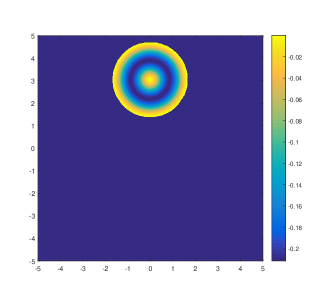
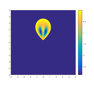
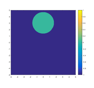
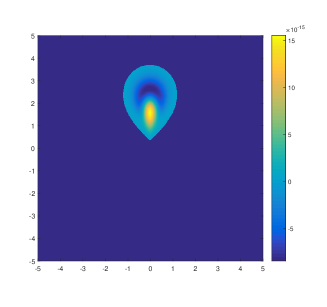
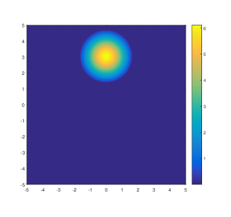
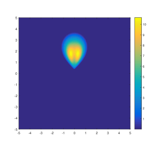
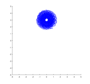
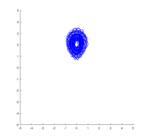
Figure 1: (From top to bottom) Pressure ($dyne/cm^{2}$), density ($g/cm^{3}$), magnetic field magnitude ($G$) and magnetic filed lines in unstretched(left) and stretched(right) GL torus. All horizontal and vertical axis are in $R_{\odot}$. We used $r_{0}=1.67$, $r_{1}=3.03$, $a=1.01$ and $a_{1}=0.23$ in these figures. (0,0) coordinate represents solar center.

2.3 Data-Constrained CME Model Using Graduated Cylindrical Shell Method

We utilize the Sun-Earth Connection Coronal and Heliospheric Investigation (SECCHI)/Cor1/Cor2  [Howard et al., 2008] coronagraph image data from STEREO A & B [Kaiser et al., 2008] and Large Angle Spectroscopic Coronagraph (LASCO)/C2/C3 [Brueckner et al., 1995] data from SOHO as observational data to constrain the GL flux rope parameters. We apply the GCS method to find the height ($h$), direction and half angle ($\theta$) (from the central axis to the outer edge) of the CME as shown in Figs. 2 and 3. GCS fitting is a visual fitting tool where three viewpoints of a CME from STEREO A & B and SOHO coronagraphs are used to fit the flux rope structure with conical legs and curved fronts over a CME. The GCS method was implemented in IDL using the rtsccguicloud program [Thernisien et al., 2006]. The size parameters of a GL flux rope $r_{0}$, $r_{1}$, and $a$ can be approximately related to the GCS size parameters according to the geometry shown in Fig. 3.

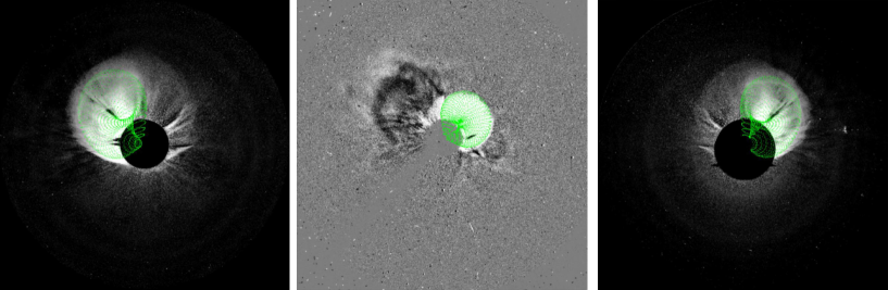
Figure 2: GCS fitting of a CME using three viewpoints: (left and right panels) SECCHI/Cor2 onboard STEREO A & B respectively, and (middle panel) LASCO/C3 onboard SOHO.

We work under the assumption that $a=r_{1}/3$ and the front edge of tear drop shape roughly matches the front end of GCS shape. In fact, by comparing the curved fronts of the tear drop and GCS shapes, we find that if we vary $r_{0}$ from $0.4$ to 2 $R_{\odot}$ and $r_{1}$ from 1.5 to 5 $R_{\odot}$, the maximum distance between the two shapes is always less than 5% of $r_{1}$. Therefore, the two shapes coincide very well. Therefore,

$$h+a=r_{1}+r_{0},$$ (12)

$$h-r_{0}=\frac{2}{3}r_{1},$$ (13)

$$h-r_{1}\,\mathop{\rm sin}\nolimits\theta=\frac{2}{3}r_{1}.$$ (14)

This gives us:

$$r_{1}=\frac{h}{2/3\,+\mathop{\rm sin}\nolimits\theta};\quad a=\frac{h}{2+3\mathop{\rm sin}\nolimits\theta};\quad r_{0}=\frac{h\,\mathop{\rm sin}\nolimits\theta}{2/3\,+\mathop{\rm sin}\nolimits\theta}.$$ (15)

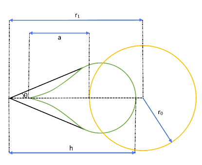
Figure 3: A diagram showing the GL sphere (yellow), its stretched tear drop shape (green), and GCS fit outline (black).

We notice that this approach constrains us to using the relation $r_{0}=r_{1}\mathop{\rm sin}\nolimits\theta$. However, $r_{1}$ and $r_{0}$ are independent parameters in GL analytical formulae. Therefore, the dependence of $r_{0}$ on $r_{1}$ is only due to the observational limitations.

The remaining GL parameter (i.e. magnetic field strength, $a_{1}$) can not be determined from observations directly. Therefore, we perform a parametric study to find an expression for $a_{1}$ in terms of $r_{0},\,r_{1}$, the average simulated solar wind pressure above the erupting region, $P_{\mathrm{avg}}$, and speed of a CME, $V_{\mathrm{CME}}$. The latter can be found by applying linear fitting to the height vs. time data from the GCS method. In order to calculate $P_{\mathrm{avg}}$, we find average pressure in simulated solar wind in $\pm 30^{\circ}$ latitude and longitude from inner boundary to 10 $R_{\odot}$.

2.3.1 Parametric Study

We follow the method used by Jin et al. [2017a] to perform the parametric study. Here, we check the effect of changes in the input GL flux rope parameters on the CME speed. In contrast to Jin et al. [2017a], we additionally allow variations in $r_{1}$. There is also a possibility of using GCS size parameters for parametric study but, as we will show below, using GL size parameters gives results in form of simple linear functions. To perform the parametric study, we need to select a magnetogram with multiple active regions. At least one of the active regions should have ejected a CME in such a direction that the CME parameters can be easily determined by the GCS method. In this study, we select the HMI LOS magnetogram from 7 March 2011 06:00 UT, in which one of the active regions numbered AR11164 produced a fast CME that occurred on 7 March 2011 at 20:00 UT. We determine the size parameters of the GL flux rope corresponding to this CME as $r_{0}=1.68$, $r_{1}=3.03$ and $a=1.01$ using the GCS method.

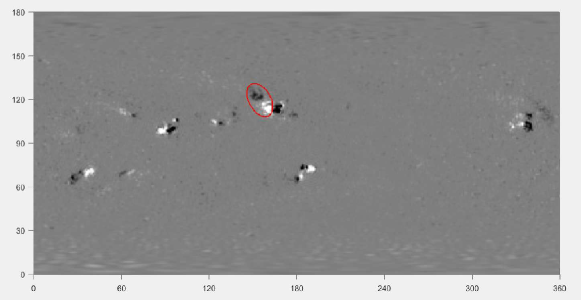
Figure 4: HMI LOS magnetogram obtained on 7 March 2011 at 06:00 UT with the source active region from which the CME erupted is indicated in red.

We perform our parametric study in three steps. First, a GL flux rope with $r_{0}=1.68$, $a_{1}=0.24$, and varying $r_{1}$ is kept on the source active region (AR11164) and the simulated CME speed is calculated (see Fig. 7). Then, we fix $r_{1}=3.03$ and the poloidal flux, $\phi$, is varied by changing $r_{0}$ and $a_{1}$ while still keeping the flux rope at the same source active region (see Fig. 5). Poloidal flux of a GL flux rope can be determined by integrating the magnitude of poloidal magnetic field component over the surface perpendicular to the polar axis of GL spherical torus. It can be shown that $\phi\propto a_{1}r_{0}^{4}$ [Jin et al., 2017a]. Finally, we place the same flux rope with parameters $r_{0}=1.68$, $a_{1}=0.18$ and $r_{1}=3.03$ over different active regions with different $P_{\mathrm{avg}}$’s and determine the variation in the simulated CME speed (see Fig. 6).

We combine all these steps to derive an expression for $a_{1}$ as follows:

$$V_{\mathrm{CME}}=f_{1}(\phi)\cdot f_{2}(P_{avg})\cdot f_{3}(r_{1}).$$ (16)

The parametric study shows that $f_{1}$ and $f_{2}$ are linear functions whereas $f_{3}$ is linear for $r_{1}<2.6$ and constant for $r_{1}>=2.6$. There is an explanation for the latter behavior. When we keep the stretched GL flux rope closer to the Sun, most of its lower part resides under solar surface and full energy of the GL flux rope is therefore not injected into the background solar wind. We also note that Jin et al. [2017a] use active region magnetic field strength $B_{r}$ instead of $P_{\mathrm{avg}}$ to differentiate between different locations where flux rope is kept initially. We find that $P_{\mathrm{avg}}$ shows much better correlation with $V_{\mathrm{CME}}$ than $B_{r}$.

Keeping the above in mind, we can write out:

$$V_{\mathrm{CME}}=\begin{cases}(c_{1}a_{1}r_{0}^{4}+c_{2})\cdot(c_{3}P_{avg}+c_{4})\cdot(c_{5}r_{1}+c_{6})&r_{1}<2.6\\ (c_{1}a_{1}r_{0}^{4}+c_{2})\cdot(c_{3}P_{avg}+c_{4})&r_{1}\geq 2.6\end{cases}$$ (17)

Now, we use non-linear multi-variable regression on all the CME runs in the parametric study to find the fitting constants. The results are given in Table 1. Finally, the expression for $a_{1}$ can be written as follows:

$$a_{1}=\begin{cases}\frac{1}{c_{1}r_{0}^{4}}\cdot\Big{(}\frac{V_{\mathrm{CME}}}{(c_{3}P_{avg}+c_{4})\cdot(c_{5}r_{1}+c_{6})}-c_{2}\Big{)}&r_{1}<2.6\\ \frac{1}{c_{1}r_{0}^{4}}\cdot\Big{(}\frac{V_{\mathrm{CME}}}{(c_{3}P_{avg}+c_{4})}-c_{2}\Big{)}&r_{1}\geq 2.6\end{cases}$$ (18)

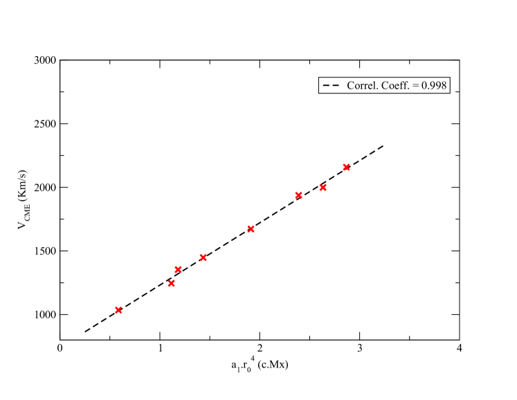
Figure 5: Variation of CME speed with poloidal flux ($\phi\propto a_{1}r_{0}^{4}$).

Figure 6: Variation of CME speed with $P_{\mathrm{avg}}$.

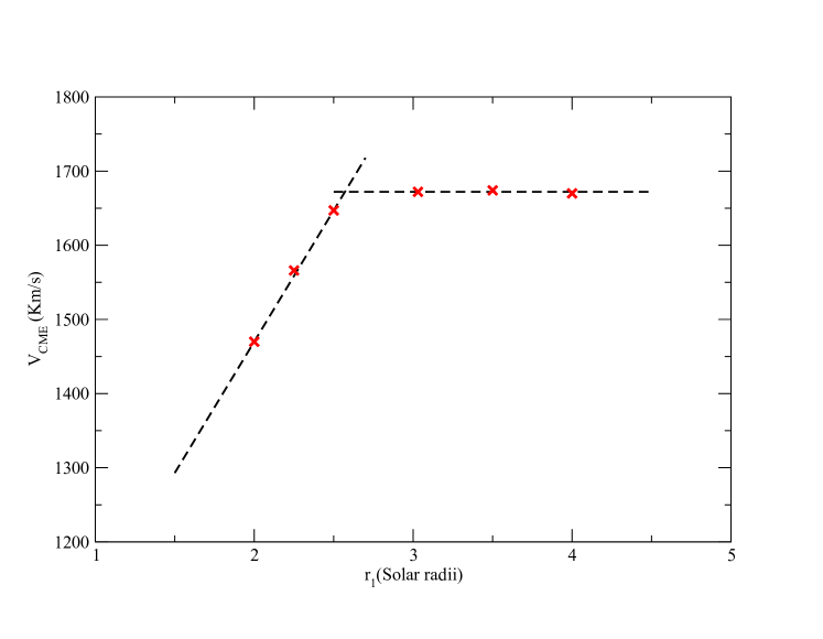
Figure 7: Variation of CME speed with $r_{1}$.

$r_{1}$	$c_{1}$	$c_{2}$	$c_{3}$	$c_{4}$	$c_{5}$	$c_{6}$
$<$ 2.6	3.849	5.831	-6.018	15.112	2.783	6.009
$\geq$ 2.6	13.018	19.721	-20.354	51.112

Table 1: Parameters used in the expression of $a_{1}$.

3 Simulation Results

In this section, we show the results related to our simulation of the eruption of the fast CME that occurred on 7 March 2011 at 20:00 UT. The background solar wind solution is obtained by relaxing the initial PFSS magnetic field distribution to steady state using our data-driven MHD global solar corona model. We computed the initial conditions for magnetic field corresponding to the simulation made to obtain the background solar wind solution from the PFSS model by using the spherical harmonics coefficients corresponding to the HMI LOS magnetogram on 7 March 2011 obtained from the pfss_viewer program on IDL SolarSoft. The initial conditions for the remaining hydrodynamic plasma variables were obtained from Parker’s isothermal solar wind model. We used the TVD, finite volume Rusanov scheme [Kulikovskii et al., 2001] to compute the numerical fluxes and the forward Euler scheme for time integration. In order to satisfy the solenoidal constraint, we applied Powell’s source term method [Powell et al., 1999]. Our computational domain size is 1.03$R_{\odot}\leq$ r $\leq 30R_{\odot}$, $0\leq\phi\leq 2\pi$, $0\leq\theta\leq\pi$ and grid size is 180$\times$240$\times$120 in r, $\phi$ and $\theta$ directions, respectively. We perform all simulations in the frame corotating with the Sun. MSFLUKSS provides us with parallel implementation of the numerical methods. At the inner boundary of the computational domain which is located at the lower corona, we applied the radial magnetic field derived from the HMI LOS magnetogram data and the differential rotation [Komm et al., 1993a] and meridional flow [Komm et al., 1993b] formulae for the horizontal velocity components at the ghost cell centers. We kept density and temperature constant as $n=1.5\times 10^{8}\,\textrm{cm}^{-3}$ and $T=1.3\times 10^{6}$ K, respectively. The radial velocity component is imposed to be zero at the boundary surface. The transverse magnetic field components are extrapolated from the domain into the ghost cells. At the outer boundary of the domain which is located beyond the critical point, the plasma flow is superfast magnetosonic, so no boundary conditions are required. The computational domain, grid size, numerical methods and boundary conditions are the same for all the runs performed. Figure 8 shows the background through which we propagate the CME.

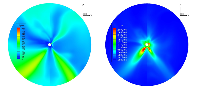
Figure 8: Solar wind background simulated using HMI LOS magnetogram of 7 March 2011 06:00 UT: (left) speed contours (km/s); (right) temperature contours (K). Background is shown in the plane in which flux rope is introduced.

We use $V_{\mathrm{CME}}$=2125 km/s for the fast CME that occurred on 7 March 2011 as given by the SOHO CME catalog [Gopalswamy et al., 2009]. We also found $r_{0}=1.68$, $r_{1}=3.03$ and $a=1.01$ from the GCS method for this CME. The pressure $P_{\mathrm{avg}}$ is found to be 0.652 mdyne/cm². Using these values and the calculated coefficients in Table 1 in Eq. 18, we find $a_{1}=0.35$. Running our simulation with this value of $a_{1}$ and the GL size parameters, we find the simulated speed to be 2140 km/s which is very close to the actual speed. Figure 9 shows the time evolution of simulated CME using temperature contours whereas Fig. 10 shows the same time evolution using magnetic flux rope structure of the CME. Figures 11 and 12 shows the comparison of the simulated CME shape with the coronagraph observations. The shape of CME is approximated by an iso-surface of the temperature.

Figure 13 shows the shock surface propagating in front of the CME. Its surface is colored according to speed values. The shock surface is found by locating the jump in entropy along radial direction with a resolution of 2^∘ in latitude and longitude. Shock properties derived from our simulation can be used to model SEP events. Hu et al. [2018] have recently used CME driven shocks to model SEP acceleration using their improved Particle Acceleration and Transport in the Heliosphere (iPATH) model. However, they note that more realistic treatment of CMEs in simulations, like using flux rope models, can enhance the accuracy of their results and better understand the SEP events.

Finally, Fig. 14 shows the agreement between the height vs. time graphs obtained from the LASCO/C3 observations and the simulation results.

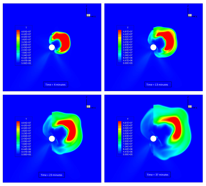
Figure 9: Time evolution of the CME shown using temperature contours.

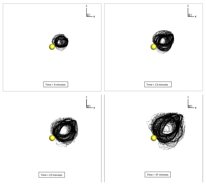
Figure 10: Time evolution of the CME shown using magnetic field lines of flux rope.

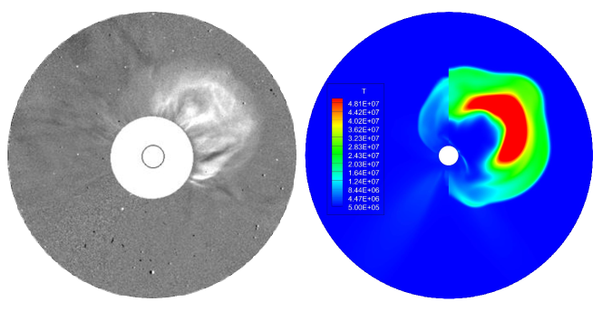
Figure 11: Comparison of CME shapes: (left panel) LASCO/C3 coronagraph difference image; (right panel) temperature contours obtained from the simulation.

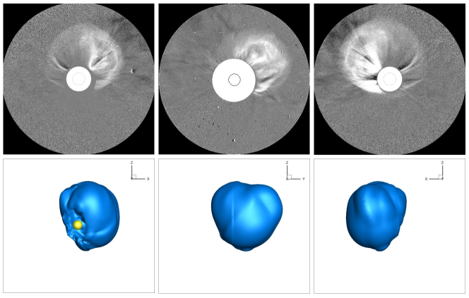
Figure 12: Comparison of CME shapes from points of view of SOHO, STEREO A & B: (upper row) From left to right: Cor2 (STEREO B), LASCO/C3, Cor2 (STEREO A); (lower row) Temperature Iso-surface indicating the CME shape in the same orientation as the corresponding image in the upper row and having same scales.

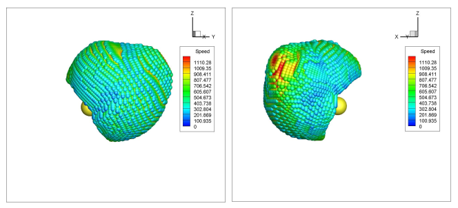
Figure 13: Shock surface in front of the simulated CME from two different viewpoints at 23 minutes after eruption.

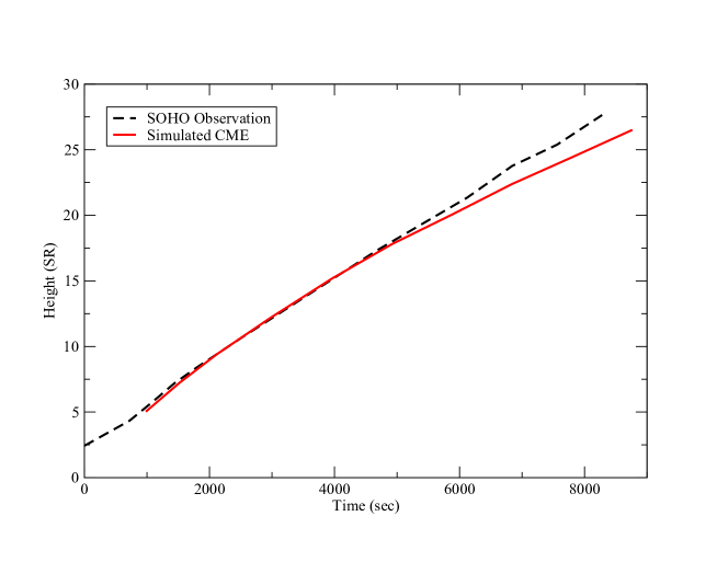
Figure 14: Comparison of height vs.time graphs between LASCO/C3 observations and simulation results.

4 Conclusions

In this paper, we presented a data-constrained CME model which is based on the GL flux rope approach and uses the GCS method. Our CME model is complementary to the model described in Jin et al. [2017b] and has certain advantages over it. We determine the GL flux rope size parameters more accurately because of the application of the GCS method to SOHO/LASCO/C2/C3 and STEREO A & B/SECCHI/Cor1/Cor2 coronagraph image data. Thus, we do not impose excessive energy in the initial flux rope configuration thereby avoiding excessive heating and acceleration of the flux rope. Determining the size parameters from the GCS method results in a realistic initial flux rope size in agreement with the observations, which leads to correct CME speed and acceleration.

These results do not imply that our CME model is better than models involving energy buildup before eruption [e.g. Titov et al., 2018, Amari et al., 2014]. However, due to its simplicity, our approach is less time consuming. Besides, it has obvious advantages over the “blob” and “cone” models because of a more realistic treatment of magnetic field.

Now when it is demonstrated that our data-constrained CME generation model works in the solar corona, we will propagate the same CME through the inner heliosphere and compare our simulation results with the near-Earth spacecraft data at 1 AU. We also plan to investigate CME-CME interactions in the future following a simulation approach.

The authors acknowledge the support from the NASA project NNX14AF41G and NSF SHINE grant AGS-1358386. This work is also supported by the Parker Solar Observatory contract with the Smithsonian Astrophysical Observatory through subcontract SV4-84017. We also acknowledge NSF PRAC award ACI-1144120 and related computer resources from the Blue Waters sustained-petascale computing project. Supercomputer allocations were also provided on SGI Pleiades by NASA High-End Computing Program award SMD-16-7570 and on Stampede2 by NSF XSEDE project MCA07S033.

This work utilizes data from SOHO which is a project of international cooperation between ESA and NASA. The HMI data have been used courtesy of NASA/SDO and HMI science teams. The STEREO/SECCHI data used here were produced by an international consortium of the Naval Research Laboratory (USA), Lockheed Martin Solar and Astrophysics Lab (USA), NASA Goddard Space Flight Center (USA), Rutherford Appleton Laboratory (UK), University of Birmingham (UK), Max-Planck-Institut for Solar System Research (Germany), Centre Spatiale de Liège (Belgium), Institut d’Optique Théorique et Appliquée (France), and Institut d’Astrophysique Spatiale (France). This work uses SOHO CME catalog which is generated and maintained at the CDAW Data Center by NASA and The Catholic University of America in cooperation with the Naval Research Laboratory.

References

- Adhikari et al. [2015] Adhikari, L., Zank, G. P., Bruno, R., et al. 2015, apj, 805, 63
- Altschuler & Newkirk [1969] Altschuler, M. D., & Newkirk, G. 1969, solphys, 9, 131
- Amari et al. [2011] Amari, T., Aly, J.-J., Luciani, J.-F., et al. 2011, apj, 742, L27
- Amari et al. [2014] Amari, T., Canou, A., & Aly, J.-J. 2014, nat, 514, 465
- Antiochos et al. [1999] Antiochos, S. K., DeVore, C. R., & Klimchuk, J. A. 1999, apj, 510, 485
- Aulanier et al. [2010] Aulanier, G., Torok, T., Demoulin, P., et al. 2010, apj, 708, 314
- Aulanier [2013] Aulanier, G. 2013, Proceeding of IAU, Volume 8, Issue S300, pp. 184-196
- Borovikov et al. [2009] Borovikov, S. N., Kryukov, I. A. & Pogorelov, N. V. 2009, in ASTRONUM 2008, Numerical Modeling of Space Plasma Flows, eds. N. V. Pogorelov, E. Audit, P. Colella, & G. P. Zank (ASP Conf. Ser. 406; San Francisco: ASP), 127
- Borovikov et al. [2013] Borovikov, S. N., Heerikhuisen, J., & Pogorelov, N. V. 2013, in ASTRONUM 2012, Numerical Modeling of Space Plasma Flows, eds. N. V. Pogorelov, E. Audit, & G. P. Zank (ASP Conf. Ser. 474; San Francisco: ASP), 219
- Borovikov et al. [2017] Borovikov, D., Sokolov, I. V., Manchester, W. B., et al. 2017, jgr, 122, 7979
- Brueckner et al. [1995] Brueckner, G. E., Howard, R. A., Koomen, M. J., et al. 1995, solphys, 162, 357
- Brueckner et al. [1998] Brueckner, G. E., Delaboudiniere, J.-P., Howard, R. A., et al. 1998, grl, 25, 3019
- Chane et al. [2005] Chane, E., Jacobs, C., van der Holst, B., et al. 2005, aap, 432, 331
- Chen [2011] Chen, P. F. 2011, Living Rev. Sol. Phys., 8, 1
- Cheung et al. [2015] Cheung, M.C. M., Pontieu, B. D., Tarbell, T. D., et al. 2015, apj, 801:83
- Cohen [2015] Cohen, O. Sol Phys (2015) 290: 2245
- Colella et al. [2007] Colella, P., Bell, J., Keen, N., et al. 2007, in Journal of Physics: Conf. Series, 78, 012013
- Detman et al. [2011] Detman, T. R., Intriligator, D. S., Dryer, M., et al. 2011, jgr, 116, 3105
- Domingo et al. [1995] Domingo, V., Fleck, B., & Poland, A. I. 1995, solphys, 162, 1
- Fan & Gibson [2007] Fan, Y., & Gibson, S. E. 2007, apj, 668, 1232
- Feng et al. [2010] Feng, X., Yang, L., Xiang, C., et al. 2010, apj, 723, 300
- Feng et al. [2011] Feng, X., Zhang, S., Xiang, C., et al. 2011, apj, 734, 50
- Feng et al. [2015] Feng, X., Ma, X., & Xiang, C. 2015, jgr, 120, 10159
- Forbes & Priest [1995] Forbes, T. G., & Priest, E. R. 1995, apj, 446, 377
- Forbes et al. [2006] Forbes, T. G., Linker, J. A., Chen, J., et al. 2006, ssr, 123, 251
- Fisher et al. [2015] Fisher, G. H., Abbett, W. P., Bercik, D. J., et al. 2015, Space Weather, 13, 6, 369-373
- Gamayunov et al. [2012] Gamayunov, K. V., Zhang, M., Pogorelov, N. V., et al. 2012, apj, 757, 74
- Gibson & Fan [2006] Gibson, S. E., & Fan, Y. 2006, jgr, 111, A12103
- Gibson & Low [1998] Gibson, S. E., & Low, B. C. 1998, apj, 493, 460
- Gopalswamy et al. [2005] Gopalswamy, N., Lara, A., Manoharan, P. K., et al. 2005, asr, 36, 2289
- Gopalswamy et al. [2009] Gopalswamy, N., Yashiro, S., Michalek, G., et al. 2009, Earth Moon Planets, 104, 295
- Hayashi [2013] Hayashi, K. 2013, jgr, 118, 6889
- Hoeksema [1984] Hoeksema, J. T. 1984, Structure and Evolution of the Large Scale Solar and Heliospheric Magnetic Fields, PhD Thesis, (Stanford University)
- Howard et al. [2008] Howard, R. A., Moses, J. D., Vourlidas, A., et al. 2008, ssr, 136, 67
- Hu [2001] Hu, Y. Q. 2001, solphys, 200, 115
- Hu et al. [2018] Hu, J., Li, G., Fu, S., 2018, apjl , 854:L19
- Intriligator et al. [2012] Intriligator, D. S., Detman, T., Gloecker, C., et al. 2012, jgr, 117, A06104
- Jacobs et al. [2006] Jacobs, C., Poedts, S., & van der Holst, B. 2006, aap, 450, 793
- Jiang et al. [2016] Jiang, C., Wu, S. T., Feng, X., et al. 2016, Nature Comm., 7, 11522
- Jin et al. [2016] Jin, M., Schrijver, C. J., Cheung, M. C. M., et al. 2016, apj, 820, 16
- Jin et al. [2017a] Jin, M., Manchester, W. B., van der Holst, B., et al. 2017, apj, 834, 172
- Jin et al. [2017b] Jin, M., Manchester, W. B., van der Holst, B., et al. 2017, apj, 834, 173
- Kaiser et al. [2008] Kaiser, M. L., Kucera, T. A., Davila, J. M., et al. 2008, ssr, 136, 5
- Kataoka et al. [2009] Kataoka, R., Ebisuzaki, K., Kusano, K., et al. 2009, jgr, 114, A10102
- Kliem & Torok [2006] Kliem, B., & Torok, T. 2006, prl, 96, 255002
- Komm et al. [1993a] Komm, R. W., Howard, R. F., & Harvey, J. W. 1993, solphys, 143, 19
- Komm et al. [1993b] Komm, R. W., Howard, R. F., & Harvey, J. W. 1993, solphys, 147, 207
- Kryukov et al. [2012] Kryukov, I. A., Pogorelov, N. V., Zank, G. P., et al. 2012, in Proceedings of the 10th Annual International Astrophysics Conference, eds. J. Heerikhuisen, G. Li, N. V. Pogorelov, & G. P. Zank (AIP Conf. Ser. 1436), 48
- Kulikovskii et al. [2001] Kulikovskii, A. G., Pogorelov, N. V., & Semenov, A. Y. 2001, Mathematical Aspects of Numerical Solution of Hyperbolic Systems, (Boca Raton: Chapman & Hall/CRC Press)
- Leake et al. [2014] Leake, J. E., Linton, M. G. & Antiochos, S. K. 2014, apj, 787, 46
- Lee et al. [2014] Lee, E., Lukin, V. S. & Linton, M. G. 2014, aap, 569, A94
- Lin & Forbes [2000] Lin, J., & Forbes, T. G. 2000, jgr, 105, 2375
- Linker & Mikic [1995] Linker, J. A., & Mikic, Z. 1995, apj, 438, L45
- Linker et al. [2016] Linker, J. A., Caplan, R. M., Downs, C., et al. 2016, in ASTRONUM 2015, Journal of Physics: Conference Series, 719, 012012
- Lionello et al. [2009] Lionello, R., Linker, J. A., & Mikic, Z. 2009, apj, 690, 902
- Lionello et al. [2016] Lionello, R., Torok, T., Titov, V. S., et al. 2016, apjl, 831, L2
- Liu et al. [2013] Liu, Y., Zhao, J., & Schuck, P. W. 2013, solphys, 287, 279
- Liu et al. [2014] Liu, Y., Hoeksema, J. T., & Sun, X. 2014, apj, 783, L1
- Liu et al. [2017] Liu, Y., Hoeksema, J. T., Sun, X., et al. 2017, solphys, 292, 29
- Lockwood et al. [2016] Lockwood, M., Owens M. J., Barnard L. A., et al. 2016, Space Weather, 14, 406–432,
- Lugaz et al. [2005] Lugaz, N., Manchester IV, W. B. & Gombosi, T. I. 2005, apj, 634, 651
- Lugaz et al. [2007] Lugaz, N., Manchester, W. B. & Toth, G. 2007, apj, 659, 788
- Lugaz & Roussev [2011] Lugaz, N., & Roussev, I. I. 2011, jastp, 73, 1187
- Lugaz et al. [2017] Lugaz, N., Temmer, M., Wang, Y., et al. 2017, solphys, 292, 64
- Manchester et al. [2004a] Manchester, W. B., Gombosi, T. I., Roussev, I., et al. 2004, jgr, 109, 2107
- Manchester et al. [2004b] Manchester, W. B., Gombosi, T. I., Roussev, I., et al. 2004, jgr, 109, 1102
- Manchester et al. [2006] Manchester, W. B., Ridley, A. J., Gombosi, T. I., et al. 2006, asr, 38, 253
- Manchester et al. [2014a] Manchester IV, W. B., Kozyra, J. U., Lepri, S. T., et al. 2014, jgr, 119, 5449
- Manchester et al. [2014b] Manchester IV, W. B., van der Holst, B., & Lavraud, B. 2014, ppcf, 56, 064006
- Manoharan et al. [2004] Manoharan, P. K., Gopalswamy, N., Yashiro, S., et al. 2004, jgr, 109, A06109
- Merkin et al. [2016] Merkin, V. G., Lionello, R., Lyon, J. G., et al. 2016, apj, 831, 23
- Mikic & Linker [1994] Mikic, Z., & Linker, J. A. 1994, apj, 430, 898
- Moon [2002] Moon, Y.-J., Dryer, M., Smith, Z., et al. 2002, grl, 29, 1390
- Moore et al. [2001] Moore, R. L., Sterling, A. C., Hudson, H. S., et al. 2001, apj, 552, 833
- Nakamizo et al. [2009] Nakamizo, A., Tanaka, T., Kubo, Y., et al. 2009, jgr, 114, A07109
- Odstrcil & Pizzo [1999a] Odstrcil, D., & Pizzo, V. J. 1999, jgr, 104, 483
- Odstrcil & Pizzo [2009] Odstrcil, D., & Pizzo, V. J. 2009, solphys, 259, 297
- Oran et al. [2015] Oran, R., Landi, E., van der Holst, B., et al. 2015, apj, 806, 55
- Parker [1958] Parker, E. N. 1958, apj, 128, 664
- Poedts & Pomoell [2017] Poedts, S., & Pomoell, J. 2017, in Proceedings of the 19th EGU General Assembly Conference Abstracts, EGU General Assembly, Vienna, 19, 7396
- Pesnell et al. [2012] Pesnell, W. D., Thompson, B. J., & Chamberlin, P. C. 2012, solphys, 275, 3
- Pogorelov et al. [2009] Pogorelov, N. V., Borovikov, S. N., Florinski, V., et al. 2009, in ASTRONUM 2008, Numerical Modeling of Space Plasma Flows, eds. N. V. Pogorelov, E. Audit, P. Colella, & G. P. Zank (ASP Conf. Ser. 406; San Francisco: ASP), 149
- Pogorelov et al. [2013] Pogorelov, N. V., Borovikov, S. N., Bedford, M. C., et al. 2013, in ASTRONUM 2012, Numerical Modeling of Space Plasma Flows, eds. N. V. Pogorelov, E. Audit, & G. P. Zank (ASP Conf. Ser. 474; San Francisco: ASP), 165
- Pogorelov et al. [2014] Pogorelov, N. V., Borovikov, S. N., Heerikhuisen, J., et al. 2014, in XSEDE’14 Proceedings of the 2014 Annual Conference on Extreme Science and Engineering Discovery Environment (ACM: New York), 22
- Pogorelov et al. [2017] Pogorelov, N. V., Borovikov, S. N., Kryukov, I. A., et al. 2017, in IOP Conf. Series: Journal of Physics: Conf. Series, 837, 012014
- Pomoell et al. [2017] Pomoell, J., Kilpua, E., Verbeke, C., et al. 2017, in Proceedings of the 19th EGU General Assembly Conference Abstracts, EGU General Assembly, Vienna, 19, 11747
- Powell et al. [1999] Powell, K. G., Roe, P. L., Linde, T. J., et al. 1999, jcp, 154, 284
- Riley et al. [2003] Riley, P., Mikic, Z., & Linker, J. A. 2003, ag, 21, 1347
- Riley et al. [2015a] Riley, P., Linker, J. A., & Arge, C. N. 2015, spwea, 13, 1
- Riley et al. [2015b] Riley, P., Lionello, R., Linker, J. A., et al. 2015, apj, 802, 105
- Riley & Richardson [2013] Riley, P., & Richardson, I. G. 2013, solphys, 284, 217
- Roussev et al. [2003b] Roussev, I. I., Gombosi, T. I., Sokolov, I. V. et al. 2003, apj, 595, L57
- Roussev et al. [2012] Roussev, I. I., Galsgaard, K., Downs, C., et al. 2012, natphys, 8, 845
- Schatten et al. [1969] Schatten, K. H., Wilcox, J. M., & Ness, N. F. 1969, solphys, 6, 442
- Schatten et al. [1969] Schatten, K. H., Wilcox, J. M., & Ness, N. F. 1969, solphys, 6, 442
- Scherrer et al. [1995] Scherrer, P. H., Bogart, R. S., Bush, R. I., et al. 1995, solphys, 162, 129
- Schmieder et al. [2015] Schmieder, B., Aulanier, G., & Vrsnak, B. 2015, solphys, 290, 3457
- Schou et al. [2012] Schou, J., Scherrer, P. H., Bush, R. I., et al. 2012, solphys, 275, 229
- Schrijver & DeRosa [2003] Schrijver, C. J., & DeRosa, M. L. 2003, solphys, 212, 165
- Schuck [2008] Schuck, P. W. 2008, apj, 683, 1134
- Shen et al. [2017] Shen, F., Wang, Y., Shen, C., et al. 2017, solphys, 292, 104
- Shiota & Kataoka [2016] Shiota, D., & Kataoka, R. 2016, spwea, 14, 56
- Sokolov et al. [2013] Sokolov, I. V., van der Holst, B., Oran, R., et al. 2013, apj, 764, 23
- Thernisien et al. [2006] Thernisien, A. F. R., Howard, R. A., & Vourlidas, A. 2006, apj, 652, 763
- Titov & Demoulin [1999] Titov, V. S., & Demoulin, P. 1999, aap, 351, 707
- Titov et al. [2014] Titov, V. S., Torok, T., Mikic, Z., et al. 2014, apj, 790, 163
- Torok & Kliem [2005] Torok, T., & Kliem, B. 2005, apjl, 630, L97
- Torok et al. [2004] Torok, T., Kliem, B., & Titov, V. S. 2004, aap, 413, L27
- Toth et al. [2011] Toth, G., van der Holst, B., & Huang, Z. 2011, apj, 732, 102
- Usmanov & Goldstein [2006] Usmanov, A. V., & Goldstein, M. L. 2006, jgr, 111, A07101
- Usmanov et al. [2011] Usmanov, A. V., Matthaeus, W. H., Breech, B. A., et al. 2011, apj, 727, 84
- Vandas et al. [1996] Vandas M., Fischer, S., Dryer, M., et al. 1996, jgr, 101, 15645
- van der Holst et al. [2014] van der Holst, B., Sokolov, I. V., Meng, X., et al. 2014, apj, 782, 81
- Vrsnak [2001] Vrsnak B. 2001, solphys, 202, 173
- Vrsnak & Gopalswamy [2002] Vrsnak, B., & Gopalswamy, N. 2002, jgr, 107, SSH 2-1
- Wang & Sheeley [1992] Wang, Y.-M., & Sheeley, N. R., Jr. 1992, apj, 392, 310
- Wang & Sheeley [1997] Wang, Y.-M., & Sheeley, N. R., Jr. 1997, grl, 24, 3141
- Wang et al. [2002] Wang, Y. M., Ye, P. Z., Wang, S., et al. 2002, jgr, 107, SSH 2-1
- Wang et al. [2011] Wang, A. H., Wu, S. T., Tandberg-Hanssen, E., et al. 2011, apj, 732, 19
- Wu et al. [2009] Wu, S. T., Wang, A. H., Gary, G. A., et al. 2009, asr, 44, 46
- Yalim et al. [2017] Yalim, M. S., Pogorelov, N. V., & Liu, Y. 2017, in IOP Conf. Series: Journal of Physics: Conf. Series, 837, 012015
- Zhao et al. [2012] Zhao, J., Couvidat, S., Bogart, R. S., et al. 2012, solphys, 275, 375
- Titov et al. [2018] Titov,V. S., Downs , C., Mikić, Z., Török, T., Linker, J. A., & Caplan,R. M.