JLAB-PHY-18-2760

SLAC–PUB–17279

The Spin Structure of the Nucleon

Alexandre Deur

Thomas Jefferson National Accelerator Facility, Newport News, VA 23606, USA

Stanley J. Brodsky

SLAC National Accelerator Laboratory, Stanford University, Stanford, CA 94309, USA

Guy F. de Téramond

Laboratorio de Física Teórica y Computacional, Universidad de Costa Rica, San José, Costa Rica

deurpam@jlab.org,

sjbth@slac.stanford.edu,   gdt@asterix.crnet.cr,

Abstract

We review the present understanding of the spin structure of protons and neutrons, the fundamental building blocks of nuclei collectively known as nucleons. The field of nucleon spin provides a critical window for testing Quantum Chromodynamics (QCD), the gauge theory of the strong interactions, since it involves fundamental aspects of hadron structure which can be probed in detail in experiments, particularly deep inelastic lepton scattering on polarized targets.

QCD was initially probed in high energy deep inelastic lepton scattering with unpolarized beams and targets. With time, interest shifted from testing perturbative QCD to illuminating the nucleon structure itself. In fact, the spin degrees of freedom of hadrons provide an essential and detailed verification of both perturbative and nonperturbative QCD dynamics.

Nucleon spin was initially thought of coming mostly from the spin of its quark constituents, based on intuition from the parton model. However, the first experiments showed that this expectation was incorrect. It is now clear that nucleon physics is much more complex, involving quark orbital angular momenta as well as gluonic and sea quark contributions. Thus, the nucleon spin structure remains a most active aspect of QCD research, involving important advances such as the developments of generalized parton distributions (GPD) and transverse momentum distributions (TMD).

Elastic and inelastic lepton-proton scattering, as well as photoabsorption experiments provide various ways to investigate non-perturbative QCD. Fundamental sum rules – such as the Bjorken sum rule for polarized photoabsorption on polarized nucleons – are also in the non-perturbative domain. This realization triggered a vigorous program to link the low energy effective hadronic description of the strong interactions to fundamental quarks and gluon degrees of freedom of QCD. This has also led to advances in lattice gauge theory simulations of QCD and to the development of holographic QCD ideas based on the AdS/CFT or gauge/gravity correspondence, a novel approach providing a well-founded semiclassical approximation to QCD. Any QCD-based model of the nucleon’s spin and dynamics must also successfully account for the observed spectroscopy of hadrons. Analytic calculations of the hadron spectrum, a long sought goal of QCD research, have now being realized using light-front holography and superconformal quantum mechanics, a formalism consistent with the results from nucleon spin studies.

We begin this review with a phenomenological description of nucleon structure in general and of its spin structure in particular, aimed to engage non-specialist readers. Next, we discuss the nucleon spin structure at high energy, including topics such as Dirac’s front form and light-front quantization which provide a frame-independent, relativistic description of hadron structure and dynamics, the derivation of spin sum rules, and a direct connection to the QCD Lagrangian. We then discuss experimental and theoretical advances in the nonperturbative domain – in particular the development of light-front holographic QCD and superconformal quantum mechanics, their predictions for the spin content of nucleons, the computation of PDFs and of hadron masses.

1 Preamble

The study of the individual contributions to the nucleon spin provides a critical window for testing detailed predictions of QCD for the internal quark and gluon structure of hadrons. Fundamental spin predictions can be tested experimentally to high precision, particularly in measurements of deep inelastic scattering (DIS) of polarized leptons on polarized proton and nuclear targets.

The spin of the nucleons was initially thought to originate simply from the spin of the constituent quarks, based on intuition from the parton model. However, experiments have shown that this expectation was incorrect. It is now clear that nucleon spin physics is much more complex, involving quark and gluon orbital angular momenta (OAM) as well as gluon spin and sea-quark contributions. Contributions to the nucleon spin, in fact, originate from the nonperturbative dynamics associated with color confinement as well as from perturbative QCD (pQCD) evolution. Thus, nucleon spin structure has become an active aspect of QCD research, incorporating important theoretical advances such as the development of GPD and TMD.

Fundamental sum rules, such as the Bjorken sum rule for polarized DIS or the Drell-Hearn-Gerasimov sum rule for polarized photoabsorption cross-sections, constrain critically the spin structure. In addition, elastic lepton-nucleon scattering and other exclusive processes, e.g. Deeply Virtual Compton Scattering (DVCS), also determine important aspects of nucleon spin dynamics. This has led to a vigorous theoretical and experimental program to obtain an effective hadronic description of the strong force in terms of the basic quark and gluon fields of QCD. Furthermore, the theoretical program for determining the spin structure of hadrons has benefited from advances in lattice gauge theory simulations of QCD and the recent development of light-front holographic QCD ideas based on the AdS/CFT correspondence, an approach to hadron structure based on the holographic embedding of light-front dynamics in a higher dimensional gravity theory, together with the constraints imposed by the underlying superconformal algebraic structure. This novel approach to nonperturbative QCD and color confinement has provided a well-founded semiclassical approximation to QCD. QCD-based models of the nucleon spin and dynamics must also successfully account for the observed spectroscopy of hadrons. Analytic calculations of the hadron spectrum, a long-sought goal, are now being carried out using Lorentz frame-independent light-front holographic methods.

We begin this review by discussing why nucleon spin structure has become a central topic of hadron physics (Section 2). The goal of this introduction is to engage the non-specialist reader by providing a phenomenological description of nucleon structure in general and its spin structure in particular.

We then discuss the scattering reactions (Section 3) which constrain nucleon spin structure, and the theoretical methods (Section 4) used for perturbative or nonperturbative QCD calculations. A fundamental tool is Dirac’s front form (light-front quantization) which, while keeping a direct connection to the QCD Lagrangian, provides a frame-independent, relativistic description of hadron structure and dynamics, as well as a rigorous physical formalism that can be used to derive spin sum rules (Section  5).

Next, in Section 6, we discuss the existing spin structure data, focusing on the inclusive lepton-nucleon scattering results, as well as other types of data, such as semi-inclusive deep inelastic scattering (SIDIS) and proton-proton scattering. Section 7 provides an example of the knowledge gained from nucleon spin studies which illuminates fundamental features of hadron dynamics and structure. Finally, we summarize in Section 8 our present understanding of the nucleon spin structure and its impact on testing nonperturbative aspects of QCD.

A lexicon of terms specific to the nucleon spin structure and related topics is provided at the end of this review to assist non-specialists. Words from this list are italicized throughout the review. Also included is a list of acronyms used in this review.

Studying the spin of the nucleon is a complex subject because light quarks move relativistically within hadrons; one needs special care in defining angular momenta beyond conventional nonrelativistic treatments [1]. Furthermore, the concept of gluon spin is gauge dependent; there is no gauge-invariant definition of the spin of gluons – or gauge particles in general [2, 3]; the definition of the spin content of the nucleon is thus dependent on the choice of gauge. In the light-front form one usually takes the light-cone gauge [1] where the spin is well defined: there are no ghosts or negative metric states in this transverse gauge (See Sec. 3.1.3). Since nucleon structure is nonperturbative, calculations based solely on first principles of QCD are difficult. These features make the nucleon spin structure an active and challenging field of study.

There are several excellent previous reviews which discuss the high-energy aspects of proton spin dynamics [4, 5, 6, 7, 8, 9, 10]. This review will also cover less conventional topics, such as how studies of spin structure illuminate aspects of the strong force in its nonperturbative domain, the consequences of color confinement, the origin of the QCD mass scale, and the emergence of hadronic degrees of freedom from its partonic ones.

It is clearly important to know how the quark and gluon spins combine with their OAM to form the total nucleon spin. A larger purpose is to use empirical information on the spin structure of hadrons to illuminate features of the strong force – arguably the least understood fundamental force in the experimentally accessible domain. For example, the parton distribution functions (PDFs) are themselves nonperturbative quantities. Quark and gluon OAMs – which significantly contribute to the nucleon spin – are directly connected to color confinement.

We will only briefly discuss some high-energy topics such as GPDs, TMDs, and the nucleon spin observables sensitive to final-state interactions such as the Sivers effect. These topics are well covered in the reviews mentioned above. A recent review on the transverse spin in the nucleon is given in Ref. [11]. These topics are needed to understand the details of nucleon spin structure at high energy, but they only provide qualitative information on our main topic, the nucleon spin [12]. For example, the large transverse spin asymmetries measured in singly-polarized lepton-proton and proton-proton collisions hint at significant transverse-spin–orbit coupling in the nucleon. This provides an important motivation for the TMD and GPD studies which constrain OAM contributions to nucleon spin.

2 Overview of QCD and the nucleon structure

The description of phenomena given by the Standard Model is based on a small number of basic elements: the fundamental particles (the six quarks and six leptons, divided into three families), the four fundamental interactions (the electromagnetic, gravitational, strong and weak nuclear forces) through which these particles interact, and the Higgs field which is at the origin of the masses of the fundamental particles. Among the four interactions, the strong force is the least understood in the presently accessible experimental domains. QCD, its gauge theory, describes the interaction of quarks via the exchange of vector gluons, the gauge bosons associated with the color fields. Each quark carries a “color” charge labeled blue, green or red, and they interact by the exchange of colored gluons belonging to a color octet.

QCD is best understood and well tested at small distances thanks to the property of asymptotic freedom [13]: the strength of the interaction between color charges effectively decreases as they get closer. The formalism of pQCD can therefore be applied at small distances; i.e., at high momentum transfer, and it has met with remarkable success. This important feature allows one to validate QCD as the correct fundamental theory of the strong force. However, most natural phenomena involving hadrons, including color confinement, are governed by nonperturbative aspects of QCD.

Asymptotic freedom also implies that the binding of quarks becomes stronger as their mutual separation increases. Accordingly, the quarks confined in a hadron react increasingly coherently as the characteristic distance scale at which the hadron is probed becomes larger: The nonperturbative distributions of all quarks and gluons within the nucleon can participate in the reaction. In fact, even in the perturbative domain, the nonperturbative dynamics which underlies hadronic bound-state structure is nearly always involved and is incorporated in distribution amplitudes, structure functions, and quark and gluon jet fragmentation functions. This is why, as a general rule, pQCD cannot predict the analytic form and magnitude of such distributions, but only their evolution with a change of scale, such as the momentum transfer of the probe. For a complete understanding of the strong force and of the hadronic and nuclear matter surrounding us (of which $\approx 95\%$ of the mass comes from the strong force), it is essential to understand QCD in its nonperturbative domain. The key example of a nonperturbative mechanism which is still not clearly understood is color confinement.

At large distances, where the internal structure cannot be resolved, effective degrees of freedom emerge; thus the fundamental degrees of freedom of QCD, quarks and gluons, are effectively replaced by baryons and mesons. The emergence of relevant degrees of freedom associated with an effective theory is a standard occurence in physics; e.g., Fermi’s theory for the weak interaction at large distances, molecular physics with its effective Van der Waals force acting on effective degrees of freedom (atoms), or geometrical optics whose essential degree of freedom is the light ray. Even outside of the field of physics, a science based on natural processes often leads to an effective theory in which the complexity of the basic phenomena is simplified by the introduction of effective degrees of freedom, sublimating the underlying effects that become irrelevant at the larger scale. For example, biology takes root from chemistry, itself based on atomic and molecular physics which in part are based on effective degrees of freedom such as nuclei. Thus the importance of understanding the connections between the fundamental theories and effective theories to satisfactorily unify knowledge on a single theoretical foundation. An important avenue of research in QCD belongs to this context: to understand the connection between the fundamental description of nuclear matter in terms of quarks and gluons and its effective description in terms of the baryons and mesons. A part of this review will discuss how spin helps with this endeavor.

QCD is most easily studied with the nucleon, since it is stable and its structure is determined by the strong force. As a first step, one studies its structure without accounting for the spin degrees of freedom. This simplifies both theoretical and experimental aspects. Accounting for spin then tests QCD in detail. This has been made possible due to continual technological advances such as polarized beams and polarized targets.

A primary way to study the nucleon is to scatter beams of particles – leptons or hadrons – on a fixed target. The interaction between the beam and target typically occurs by the exchange of a photon or a $W$ or $Z$ vector boson. The momentum of the exchanged quantum controls the time and distance scales of the probe.

Alternatively, one can collide two beams. Hadrons either constitute one or both beams (lepton-hadron or hadron-hadron colliders) or are generated during the collision ($e^{+}$–$e^{-}$ colliders). The main facilities where nucleon spin structure has been studied are SLAC in California, USA (tens of GeV electrons impinging on fixed proton or nuclear targets), CERN in France/Switzerland (hundreds of GeV muons colliding with fixed targets), DESY in Germany (tens of GeV electrons in a ring scattering off an internal gas target), Jefferson Laboratory (JLab) in Virginia, USA (electrons with energy up to 11 GeV with fixed targets), the Relativistic Heavy Ion Collider (RHIC) at Brookhaven Laboratory in New York, USA (colliding beams of protons or nuclei with energies about 10 GeV per nucleon), and MAMI (electrons of up to 1.6 GeV on fixed targets) in Germany. We will now survey the formalism describing the various reactions just described.

2.1 Charged lepton-nucleon scattering

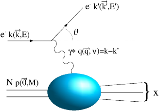
Figure 1: Inclusive electron scattering off a nucleon, in the first Born approximation. The blob represents the nonperturbative response of the target to the photon.

We start our discussion with experiments where charged leptons scatter off a fixed target. We focus on the “inclusive” case where only the scattered lepton is detected. The interactions involved in the reaction are the electromagnetic force (controlling the scattering of the lepton) and the strong force (governing the nuclear or nucleon structures). Neutrino scattering, although it is another important probe of nucleon structure, will not be discussed in detail here because the small weak interaction cross-sections, and the unavailability of large polarized targets, have so far prohibited its use for detailed spin structure studies. Nonetheless, as we shall discuss, neutrino scattering off unpolarized targets and parity-violating electron scattering yield constraints on nucleon spin [14]. The formalism for inelastic lepton scattering, including the weak interaction, can be found e.g. in Ref. [15].

2.1.1 The first Born approximation

The electromagnetic interaction of a lepton with a hadronic or nuclear target proceeds by the exchange of a virtual photon. The first-order amplitude, known as the first Born approximation, corresponds to a single photon exchange, see Fig. 1. In the case of electron scattering, where the lepton mass is small, higher orders in perturbative quantum electrodynamics (QED) are needed to account for bremsstrahlung (real photons emitted by the incident or the scattered electron), vertex corrections (virtual photons emitted by the incident electron and re-absorbed by the scattered electron) and “vacuum polarization” diagrams (the exchanged photon temporarily turning into pairs of charged particles). In some cases, such as high-$Z$ nuclear targets, it is also necessary to account for the cases where the interaction between the electron and the target is transmitted by the exchange of multiple photons (see e.g. [16]). This correction will be negligible for the reactions and kinematics discussed here. Perturbative techniques can be applied to the electromagnetic probe, since the QED coupling $\alpha\approx 1/137$, but not to the target structure whose reaction to the absorption of the photon is governed by the strong force at large distances where the QCD coupling $\alpha_{s}$ can be large.

2.1.2 Kinematics

Figure 2: Definitions of the polar angle $\theta^{*}$ and azimuthal angle $\phi^{*}$ of the target spin $\vec{S}$. The scattering plane is defined by $x\otimes z$.

In inclusive reactions the final state system $X$ is not detected. In the case of an “elastic” reaction, the target particle emerges without structure modification. Alternatively, the target nucleon or nucleus can emerge as excited states which promptly decay by emitting new particles (the resonance region), or the target can fragment, with additional particles produced in the final state as in DIS.

We first consider measurements in the laboratory frame where the nucleon or nuclear target is at rest (Figs. 1 and 2). The laboratory energy of the virtual photon is $\nu\equiv E-E^{\prime}$. The direction of the momentum $\overrightarrow{q}\equiv\overrightarrow{k}-\overrightarrow{k^{\prime}}$ of the virtual photon defines the $\overrightarrow{z}$ axis, while $\overrightarrow{x}$ is in the $(\overrightarrow{k},\overrightarrow{k^{\prime}})$ plane. $\overrightarrow{S}$ is the target spin, with $\theta^{*}$ and $\phi^{*}$ its polar and azimuthal angles, respectively. In inclusive reactions, two variables suffice to characterize the kinematics; in the elastic case, they are related, and one variable is enough.

During an experiment, the transferred energy $\nu$ and the scattering angle $\theta$ are typically varied. Two of the following relativistic invariants are used to characterize the kinematics:

$\bullet$ The exchanged 4-momentum squared $Q^{2}\equiv-(k-k^{\prime})^{2}=4EE^{\prime}\sin^{2}\frac{\theta}{2}$ for ultra-relativistic leptons. For a real photon, $Q^{2}=0$.

$\bullet$ The invariant mass squared $W^{2}\equiv(p+q)^{2}=M_{t}^{2}+2M_{t}\nu-Q^{2}$, where $M_{t}$ is the mass of the target nucleus. $W$ is the mass of the system formed after the lepton-nucleus collision; e.g., a nuclear excited state.

$\bullet$ The Bjorken variable $x_{Bj}\equiv\frac{Q^{2}}{2p.q}=\frac{Q^{2}}{2M_{t}\nu}$. This variable was introduced by Bjorken in the context of scale invariance in DIS; see Section 3.1.2. One has $0<x_{Bj}<M_{t}/M$, where $M$ the nucleon mass, since $W\geq M_{t}$, $Q^{2}>0$ and $\nu>0$.

$\bullet$ The laboratory energy transfer relative to the incoming lepton energy $y=\nu/E$.

Depending on the values of $Q^{2}$ and $\nu$, the target can emerge in different excited states. It is advantageous to study the excitation spectrum in terms of $W$ since each excited state corresponds to specific a value of $W$ rather than $\nu$, see Fig. 3.

2.1.3 General expression of the reaction cross-section

In what follow, “hadron” can refer to either a nucleon or a nucleus. The reaction cross-section is obtained from the scattering amplitude $T_{fi}$ for an initial state $i$ and final state $f$. $T_{fi}$ is computed from the photon propagator and the leptonic current contracted with the electromagnetic current of the hadron for the exclusive reaction $\ell H\to\ell^{\prime}H^{\prime}$, or a tensor in the case of an incompletely known final state. These quantities are conserved at the leptonic and hadronic vertices (gauge invariance).

Figure 3: Response of the nucleon to the electromagnetic probe as a function of $Q^{2}$ and $\nu$. The $\nu$-positions of the peaks (N, $\Delta$,…) change as $Q^{2}$ varies. (After [17].)

In the first Born approximation:

$$\vspace{-0.3cm}T_{fi}=\left\langle k^{\prime}\right|j^{\mu}(0)\left|k\right\rangle\frac{1}{Q^{2}}\left\langle P_{X}\right|J_{\mu}(0)\left|P\right\rangle,$$ (1)

where the leptonic current is $j^{\mu}=e\overline{\psi_{l}}\gamma^{\mu}\psi_{l}$ with $\psi_{l}$ the lepton spinor, $e$ its electric charge and $J^{\mu}$ the quark current. The exact expression of the hadron’s current matrix element $\left\langle P_{X}\right|J_{\mu}(0)\left|P\right\rangle$ is unknown because of our ignorance of the nonperturbative hadronic structure and, for non-exclusive experiments, that of the final state. However, symmetries (parity, time reversal, hermiticity, and current conservation) constrain the matrix elements of $J^{\mu}$ to a generic form written in terms of the vectors and tensors pertinent to the reaction. Our ignorance of the hadronic structure is thus parameterized by functions which can be either measured, computed numerically, or modeled. These are called either “form factors” (elastic scattering, see Section 3.3), “response functions” (quasi-elastic reaction, see Section 3.3.2) or “structure functions” (DIS case, see Section 3.1). A significant advance of the late 1990s and early 2000s is the unification of form factors and structure functions under the concept of GPDs. The differential cross-section $d\sigma$ is obtained from the absolute square of the amplitude (1) times the lepton flux and a phase space factor, given e.g., in Ref. [18].

2.1.4 Leptonic and hadronic tensors, and cross-section parameterization

The leptonic tensor $\eta^{\mu\nu}$ and the hadronic tensor $W^{\mu\nu}$ are defined such that $d\sigma\propto\left|T_{fi}\right|^{2}=\eta^{\mu\nu}\frac{1}{Q^{4}}W_{\mu\nu}$. That is, $\eta^{\mu\nu}\equiv\frac{1}{2}\sum j^{\mu*}j^{\nu}$, where all the possible final states of the lepton have been summed over (e.g., all of the lepton final spin states for the unpolarized experiments), and the tensor

$$\vspace{-0.3cm}W^{\mu\nu}=\frac{1}{4\pi}\int d^{4}\xi\,e^{iq_{\alpha}\xi^{\alpha}}\left\langle P\right|\left[J^{\mu\dagger}(\xi),J^{\nu}(0)\right]\left|P\right\rangle,$$ (2)

follows from the optical theorem by computing the forward matrix element of a product of currents in the proton state. The contribution to $W^{\mu\nu}$ which is symmetric in ${\mu,\nu}$ – thus constructed from the hadronic vector current – contributes to the unpolarized cross-section, whereas its antisymmetric part – constructed from the pseudo-vector (axial) current – yields the spin-dependent contribution.

In the unpolarized case; i.e., with summation over all spin states, the cross-section can be parameterized with six photoabsorption terms. Three terms originate from the three possible polarization states of the virtual photon. (The photon spin is a 4-vector but for a virtual photon, only three components are independent because of the constraint from gauge invariance. The unphysical fourth component is called a ghost photon.) The other three terms stem from the multiplication of the two tensors. They depend in particular on the azimuthal scattering angle, which is integrated over for inclusive experiments. Thus, these three terms disappear and

$$\vspace{-0.35cm}\left|T_{fi}\right|^{2}=\frac{e^{2}}{Q^{2}(1-\epsilon)}\left[(w_{RR}+w_{LL})+2\epsilon w_{ll}\right],$$ (3)

where $R$, $L$ and $l$ label the photon helicity state (they are not Lorentz indices) and
$\epsilon\equiv 1/\left[1+2\left(\nu^{2}/Q^{2}+1\right)\tan^{2}(\theta/2)\right]$ is the virtual photon degree of polarization in the $m_{e}=0$ approximation. The right and left helicity terms are $w_{RR}$ and $w_{LL}$, respectively. The longitudinal term $w_{ll}$ is non-zero only for virtual photons. It can be isolated by varying $\epsilon$ [19], but $w_{RR}$ and $w_{LL}$ cannot be separated. Thus, writing $w_{T}=w_{RR}+w_{LL}$ and $w_{L}=w_{ll}$, the cross-section takes the form:

$$\vspace{-0.3cm}d\sigma\propto\left|T_{fi}\right|^{2}=\frac{e^{2}}{Q^{2}(1-\epsilon)}\left[w_{T}+2\epsilon w_{L}\right].$$ (4)

The total unpolarized inclusive cross-section is expressed in terms of two photoabsorption partial cross-sections, $\sigma_{L}$ and $\sigma_{T}$. The parameterization in term of virtual photoabsorption quantities is convenient because the leptons create the virtual photon flux probing the target. For doubly-polarized inclusive inelastic scattering, where both the beam and target are polarized, two additional parameters are required: $\sigma_{TT}$ and $\sigma_{LT}^{\prime}$. (The reason for the prime ^′ is explained below). The $\sigma_{TT}$ term stems from the interference of the amplitude involving one of the two possible transverse photon helicities with the amplitude involving the other transverse photon helicity. Likewise, $\sigma_{LT}^{\prime}$ originates from the imaginary part of the longitudinal-transverse interference amplitude. The real part, which produces $\sigma_{LT}$, disappears in inclusive experiments because all angles defined by variables describing the hadrons produced during the reaction are averaged over. This term, however, appears in exclusive or semi-exclusive reactions, see e.g., the review [20].

2.1.5 Asymmetries

The basic observable for studying nucleon spin structure in doubly polarized lepton scattering is the cross-section asymmetry with respect to the lepton and nucleon spin directions. Asymmetries can be absolute: $A=\sigma^{\downarrow\Uparrow}-\sigma^{\uparrow\Uparrow}$, or relative: $A=(\sigma^{\downarrow\Uparrow}-\sigma^{\uparrow\Uparrow})/(\sigma^{\downarrow\Uparrow}+\sigma^{\uparrow\Uparrow})$. The $\downarrow$ and $\uparrow$ represent the leptonic beam helicity in the laboratory frame whereas $\Downarrow$ and $\Uparrow$ define the direction of the target polarization (here, along the beam direction). Relative asymmetries convey less information, the absolute magnitude of the process being lost in the ratio, but are easier to measure than absolute asymmetries or cross-sections since the absolute normalization (e.g., detector acceptance, target density, or inefficiencies) cancels in the ratio. Measurements of absolute asymmetries can also be advantageous, since the contribution from any unpolarized material present in the target cancels out. The optimal choice between relative and absolute asymmetries thus depends on the experimental conditions; see Section 3.1.7.

One can readily understand why the asymmetries appear physically, and why they are related to the spin distributions of the quarks in the nucleon. Helicity is defined as the projection of spin in the direction of motion. In the Breit frame where the massless lepton and the quark flip their spins after the interaction, the polarization of the incident relativistic leptons sets the polarization of the probing photons because of angular momentum conservation; i.e., these photons must be transversally polarized and have helicities $\pm 1$. Helicity conservation requires that a photon of a given helicity couples only to quarks of opposite helicities, thereby probing the quark helicity (spin) distributions in the nucleon. Thus the difference of scattering probability between leptons of $\pm 1$ helicities (asymmetry) is proportional to the difference of the population of quarks of different helicity. This is the basic physics of quark longitudinal polarization as characterized by the target hadron’s longitudinal spin structure function. Note also that virtual photons can also be longitudinally polarized, i.e., with helicity 0, which will also contribute to the lepton asymmetry at finite $Q^{2}$.

2.2 Nucleon-Nucleon scattering

Polarized proton–(anti)proton scattering, as done at RHIC (Brookhaven, USA), is another way to access the nucleon spin structure. Since hadron structure is independent of the measurement, the PDFs measured in lepton-nucleon and nucleon-nucleon scattering should be the same. This postulate of pQCD factorization underlies the ansatz that PDFs are universal. Several processes in nucleon-nucleon scattering are available to access PDFs, see Fig. 4. Since different PDFs contribute differently in different processes, investigating all of these reactions will allow us to disentangle the contributing PDFs. The analytic effects of evolution generated by pQCD is known at least to next-to-leading order (NLO) in $\alpha_{s}$ for these processes, which permits the extraction of the PDFs to high precision. The most studied processes which access nucleon spin structure are:

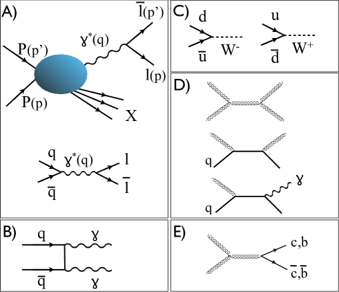
Figure 4: Various $\overrightarrow{p}\overrightarrow{p}$ reactions probing the proton spin structure. Panel A: Drell-Yan process and its underlying LO diagram. Panel B: Direct diphoton production at LO. Panel C: $W^{+/-}$ production at LO. Panel D: LO process dominating photon, pion and/or Jet production in $\overrightarrow{p}\overrightarrow{p}$ scattering. Panel E: heavy-flavor meson production at LO.

A) The Drell-Yan process A lepton pair detected in the final state corresponds to the Drell-Yan process, see Fig. 4, panel A. In the high-energy limit, this process is described as the annihilation of a quark from a proton with an antiquark from the other (anti)proton, the resulting timelike photon then converts into a lepton-antilepton pair. Hence, the process is sensitive to the convolution of the quark and antiquark polarized PDFs $\Delta q(x_{Bj})$ and $\Delta\overline{q}(x_{Bj})$. (They will be properly defined by Eq. (25).) Another process that leads to the same final state is lepton-antilepton pair creation from a virtual photon emitted by a single quark. However, this process requires large virtuality to produce a high energy lepton–anti-lepton pair, and it is thus kinematically suppressed compared to the panel A case.

An important complication is that the Drell-Yan process is sensitive to double initial-state corrections, where both the quark and antiquark before annihilation interact with the spectator quarks of the other projectile. Such corrections are “leading twist”; i.e., they are not power-suppressed at high lepton pair virtuality. They induce strong modifications of the lepton-pair angular distribution and violate the Lam-Tung relation [21].

A fundamental QCD prediction is that a naively time-reversal-odd distribution function, measured via Drell-Yan should change sign compared to a SIDIS measurement [22, 23, 24, 25]. An example is the Sivers function [26], a transverse-momentum dependent distribution function sensitive to spin-orbit effects inside the polarized proton.

B) Direct diphoton production Inclusive diphoton production $\overrightarrow{p}\overrightarrow{p}\rightarrow\gamma\gamma+X$ is another process sensitive to $\Delta q(x_{Bj})$ and $\Delta\overline{q}(x_{Bj})$. The underlying leading order (LO) diagram is shown on panel B of Fig. 4.

C) $W^{+/-}$ production The structure functions probed in lepton scattering involve the quark charge squared (see Eqs. (21) and (23)): They are thus only sensitive to $\Delta q+\Delta\overline{q}$. $W^{+/-}$ production is sensitive to $\Delta q(x_{Bj})$ and $\Delta\overline{q}(x_{Bj})$ separately. Panel C in Fig. 4 shows how $W^{+/-}$ production allows the measurement of both mixed $\Delta u\Delta\overline{d}$ and $\Delta d\Delta\overline{u}$ combinations; thus combining $W^{+/-}$ production data and data providing $\Delta q+\Delta\overline{q}$ (e.g., from lepton scattering) permits individual quark and antiquark contributions to be separated. The produced $W$ is typically identified via its leptonic decay to $\nu l$, with the $\nu$ escaping detection.

D) Photon, Pion and/or Jet production These processes are $\overrightarrow{p}\overrightarrow{p}\rightarrow\gamma+X$, $\overrightarrow{p}\overrightarrow{p}\rightarrow\pi+X$, $\overrightarrow{p}\overrightarrow{p}\rightarrow jet(s)+X$ and $\overrightarrow{p}\overrightarrow{p}\rightarrow\gamma+jet+X$. At high momenta, such reactions are dominated by either gluon fusion or gluon-quark Compton scattering with a gluon or photon in the final state; See panel D in Fig. 4. These processes are sensitive to the polarized gluon distribution $\Delta g(x,Q^{2})$.

E) Heavy-flavor meson production Another process which is sensitive to $\Delta g(x,Q^{2})$ is $D$ or $B$ heavy meson production via gluon fusion $\overrightarrow{p}\overrightarrow{p}\rightarrow D+X$ or $\overrightarrow{p}\overrightarrow{p}\rightarrow B+X$. See panel E in Fig. 4. The heavy mesons subsequently decay into charged leptons which are detected.

2.3 $e^{+}~{}e^{-}$ annihilation

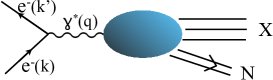
Figure 5: Annihilation of $e^{+}~{}e^{-}$ with only one detected hadron from the final state.

The $e^{+}~{}e^{-}$ annihilation process where only one hadron is detected in the final state (Fig. 5) is the timelike version of DIS if the final state hadron is a nucleon. The nucleon structure is parameterized by fragmentation functions, whose analytic form is limited – as for the spacelike case – by fundamental symmetries.

3 Constraints on spin dynamics from scattering processes

We now discuss the set of inclusive scattering processes which are sensitive to the polarized parton distributions and provide the cross-sections for each type of reaction. We start with DIS where the nucleon structure is best understood. DIS was also historically the first hard-scattering reaction which provided an understanding of fundamental hadron dynamics. Thus, DIS is the prototype – and it remains the archetype – of tests of QCD. We will then survey other inclusive reactions and explore their connection to exclusive reactions such as elastic lepton-nucleon scattering.

3.1 Deep inelastic scattering

3.1.1 Mechanism

The kinematic domain of DIS where leading-twist Bjorken scaling is valid requires $W\gtrsim 2$ GeV and $Q^{2}\gtrsim 1$ GeV². Due to asymptotic freedom, QCD can be treated perturbatively in this domain, and standard gauge theory calculations are possible. In the Bjorken limit where $\nu\to\infty$ and $Q^{2}\to\infty$, with $x_{Bj}=Q^{2}/(2M\nu)$ fixed, DIS can be represented in the first approximation by a lepton scattering elastically off a fundamental quark or antiquark constituent of the target nucleon, as in Feynman’s parton model. The momentum distributions of the quarks (and gluons) in the nucleon, which determine the DIS cross-section, reflect its nonperturbative bound-state structure. The ability to separate, at high lepton momentum transfer, perturbative photon-quark interactions from the nonperturbative nucleon structure is known as the factorization theorem [27] – a direct consequence of asymptotic freedom. It is an important ingredient in establishing the validity of QCD as a description of the strong interactions.

The momentum distributions of quarks and gluons are parameterized by the structure functions: These distributions are universal; i.e., they are properties of the hadrons themselves, and thus should be independent of the particular high-energy reaction used to probe the nucleon. In fact, all of the interactions within the nucleon which occur before the lepton-quark interaction, including the dynamics, are contained in the frame-independent light-front (LF) wave functions (LFWF) of the nucleon – the eigenstates of the QCD LF Hamiltonian. They thus reflect the nonperturbative underlying confinement dynamics of QCD; we discuss how this is assessed in models and confining theories such as Light Front Holographic QCD (LFHQCD) in Section 4.4. Final-state interactions – processes happening after the lepton interacts with the struck quark – also exist. They lead to novel phenomena such as diffractive DIS (DDIS), $\ell p\to\ell^{\prime}p^{\prime}X$, or the pseudo-T-odd Sivers single-spin asymmetry $\vec{S}_{p}\cdot\vec{q}\times\vec{p}_{q}$ which is observed in polarized SIDIS. These processes also contribute at “leading twist”; i.e., they contribute to the Bjorken-scaling DIS cross-section.

3.1.2 Bjorken scaling

DIS is effectively represented by the elastic scattering of leptons on the pointlike quark constituents of the nucleon in the Bjorken limit. Bjorken predicted that the hadron structure functions would depend only on the dimensionless ratio $x_{Bj}$, and that the structure functions reflect conformal invariance; i.e., they will be $Q^{2}$-invariant. This is in fact the prediction of “conformal” theory – a quantum field theory of pointlike quarks with no fundamental mass scale. Bjorken’s expectation was verified by the first measurements at SLAC [28] in the domain $x_{Bj}\sim 0.25$. However, in a gauge theory such as QCD, Bjorken scaling is broken by logarithmic corrections from pQCD processes, such as gluon radiation – see Section 3.1.9. One also predicts deviations from Bjorken scaling due to power-suppressed $M^{2}/Q^{2}$ corrections called higher-twist processes. They reflect finite mass corrections and hard scattering involving two or more quarks. The effects become particularly evident at low $Q^{2}$ ($\lesssim 1$ GeV²), see Section 4.1. The underlying conformal features of chiral QCD (the massless quark limit) also has important consequence for color confinement and hadron dynamics at low $Q^{2}$. This perspective will be discussed in Section 4.4.

3.1.3 DIS: QCD on the light-front

An essential point of DIS is that the lepton interacts via the exchange of a virtual photon with the quarks of the proton – not at the same instant time $t$ (the “instant form” as defined by Dirac), but at the time along the LF, in analogy to a flash photograph. In effect DIS provides a measurement of hadron structure at fixed LF time $\tau=x^{+}=t+z/c$.

The LF coordinate system in position space is based on the LF variables $x^{\pm}=(t\pm z)$. The choice of the $\hat{z}={\hat{x}}^{3}$ direction is arbitrary. The two other orthogonal vectors defining the LF coordinate system are written as $x_{\bot}=(x,y)$. They are perpendicular to the $(x^{+},x^{-})$ plane. Thus $x^{2}=x^{+}x^{-}-x_{\perp}^{2}$. Similar definitions are applicable to momentum space: $p^{\pm}=(p^{0}\pm p^{3})$, $p_{\bot}=(p_{1},p_{2})$. The product of two vectors $a^{\mu}$ and $b^{\mu}$ in LF coordinates is

$$\vspace{-0.15cm}a^{\mu}b_{\mu}=\frac{1}{2}(a^{+}b^{-}+a^{-}b^{+})-a_{\bot}b_{\bot}.$$ (5)

The relation between covariant and contravariant vectors is $a^{+}=a_{-}$, $a^{-}=a_{+}$ and the relevant metric is:

$$\left(\begin{array}[]{cccc}0&1&0&0\\ 1&0&0&0\\ 0&0&-1&0\\ 0&0&0&-1\end{array}\right).\vspace{-0.1cm}$$

Dirac matrices $\gamma^{\mu}$ adapted to the LF coordinates can also be defined [29].

The LF coordinates provide the natural coordinate system for DIS and other hard reactions. The LF formalism, called the “Front Form” by Dirac, is Poincaré invariant (independent of the observer’s Lorentz frame) and “causal” (correlated information is only possible as allowed by the finite speed of light). The momentum and spin distributions of the quarks which are probed in DIS experiments are in fact determined by the LFWFs of the target hadron – the eigenstates of the QCD LF Hamiltonian $H_{LF}$ with the Hamiltonian defined at fixed $\tau$. $H_{LF}$ can be computed directly from the QCD Lagrangian. This explains why quantum field theory quantized at fixed $\tau$ (LF quantization) is the natural formalism underlying DIS experiments. The LFWFs being independent of the proton momentum, one obtains the same predictions for DIS at an electron-proton collider as for a fixed target experiment where the struck proton is at rest.

Since important nucleon spin structure information is derived from DIS experiments, it is relevant to outline the basic elements of the LF formalism here. The evolution operator in LF time is $P^{-}=P^{0}-P^{3}$, while $P^{+}=P^{0}+P^{3}$ and $P_{\perp}$ are kinematical. This leads to the definition of the Lorentz invariant LF Hamiltonian $H_{LF}=P^{\mu}P_{\mu}=P^{-}P^{+}-P^{2}_{\perp}$. The LF Heisenberg equation derived from the QCD LF Hamiltonian is

$$\vspace{-0.3cm}H_{LF}|\Psi_{H}\rangle=M^{2}_{H}|\Psi_{H}\rangle,$$ (6)

where the eigenvalues $M_{H}^{2}$ are the squares of the masses of the hadronic eigenstates. The eigensolutions $|\Psi_{H}\rangle$ projected on the free parton eigenstates $|n\rangle$ (the Fock expansion) are the boost-invariant hadronic LFWFs, $\langle n|\Psi_{H}\rangle=\Psi_{n}(x_{i},\vec{k}_{\perp i},\lambda_{i})$, which underly the DIS structure functions. Here $x_{i}=k^{+}_{i}/P^{+}$, with $\sum_{i}x_{i}=1$, are the LF momentum fractions of the quark and gluon constituents of the hadron eigenstate in the $n$-particle Fock state, the $\vec{k}_{\perp i}$ are the transverse momenta of the $n$ constituents where $\sum_{i}\vec{k}_{\perp i}=0_{\perp}$; the variable $\lambda_{i}$ is the spin projection of constituent $i$ in the $\hat{z}$ direction.

A critical point is that LF quantization provides the LFWFs describing relativistic bound systems, independent of the observer’s Lorentz frame; i.e., they are boost invariant. In fact, the LF provides an exact and rigorous framework to study nucleon structure in both the perturbative and nonperturbative domains of QCD [30].

Just as the energy $P^{0}$ is the conjugate of the standard time $x^{0}$ in the instant form, the conjugate to the LF time $x^{+}$ is the operator $P^{-}=i\frac{d}{dx^{+}}$. It represents the LF time evolution operator

$$\vspace{-0.1cm}P^{-}\Psi=\frac{(M^{2}+P_{\bot}^{2})}{2P^{+}}\Psi,$$ (7)

and generates the translations normal to the LF.

The structure functions measured in DIS are computed from integrals of the square of the LFWFs, while the hadron form factors measured in elastic lepton-hadron scattering are given by the overlap of LFWFs. The power-law fall-off of the form factors at high-$Q^{2}$ are predicted from first principles by simple counting rules which reflect the composition of the hadron [31, 32]. One also can predict observables such as the DIS spin asymmetries for polarized targets [33].

LF quantization differs from the traditional equal-time quantization at fixed $t$ [34] in that eigensolutions of the Hamiltonian defined at a fixed time $t$ depend on the hadron’s momentum $\vec{P}$. The boost of the instant form wave function is then a complicated dynamical problem; even the Fock state structure depends on $P^{\mu}$. Also, interactions of the lepton with quark pairs (connected time-ordered diagrams) created from the instant form vacuum must be accounted for. Such complications are absent in the LF formalism. The LF vacuum is defined as the state with zero $P^{-}$; i.e., invariant mass zero and thus $P^{\mu}=0$. Vacuum loops do not appear in the LF vacuum since $P^{+}$ is conserved at every vertex; one thus cannot create particles with $k^{+}\geq 0$ from the LF vacuum.

It is sometimes useful to simulate LF quantization by using instant time in a Lorentz frame where the observer has “infinite momentum” $P^{z}\to-\infty.$ However, it should be stressed that the LF formalism is frame-independent; it is valid in any frame, including the hadron rest frame. It reduces to standard nonrelativistic Schrödinger theory if one takes $c\to\infty$. The LF quantization is thus the natural, physical, formalism for QCD.

As we shall discuss below, the study of dynamics with the LF holograpic approach which incorporates the exact conformal symmetry of the classical QCD Lagrangian in the chiral limit, provides a successful description of color confinement and nucleon structure at low $Q^{2}$ [35]. An example is given in Section 3.3.1 where nucleon form factors emerge naturally from the LF framework and are computed in LFHQCD.

Light-cone gauge

The gauge condition often chosen in the LF framework is the “light-cone” (LC) gauge defined as $A^{+}=A^{0}+A^{3}=0$; it is an axial gauge condition in the LF frame. The LC gauge is analogous to the usual Coulomb or radiation gauge since there are no longitudinally polarized nor ghosts (negative-metric) gluon. Thus, Fadeev–Popov ghosts [36] are also not required. In LC gauge one can show that $A^{-}$ is a function of $A_{\bot}$. Therefore, this physical gauge simplifies the study of hadron structure since the transverse degrees of freedom of the gluon field $A_{\bot}$ are the only independent dynamical variables. The LC gauge also insures that at LO, twist-2 expressions do not explicitly involve the gluon field, although the results retain color-gauge invariance [37]. Instead a LF-instantaneous interaction proportional to $1\over{k^{+}}^{2}$ appears in the LF Hamiltonian, analogous to the instant time instantaneous ${1}\over{\vec{k}}^{2}$ interaction which appears in Coulomb (radiation) gauge in QED.

Light-cone dominance

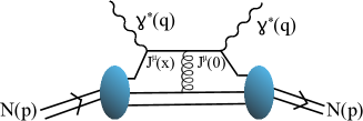
Figure 6: Forward virtual Compton scattering with a Wilson line.

Using unitarity, the hadronic tensor $W^{\mu\nu}$, Eq. (2), can be computed from the imaginary part of the forward virtual Compton scattering amplitude $\gamma^{*}(q)N(p)\to\gamma^{*}(q)N(p)$, see Fig. 6. At large $Q^{2}$, the quark propagator which connects the two currents in the DVCS amplitude goes far-off shell; as a result, the invariant spatial separation $x^{2}=x_{\mu}x^{\mu}$ between the currents $J^{\mu}(x)$ and $J^{\nu}(0)$ acting on the quark line vanishes as $x^{2}\propto{1\over Q^{2}}$. Since $x^{2}=x^{+}x^{-}-x^{2}_{\perp}\to 0$, this domain is referred to as “light-cone dominance”. The interactions of gluons with this quark propagator are referred to as the Wilson line. It represents the final-state interactions between the struck quark and the target spectators (“final-state”, since the imaginary part of the amplitude in Fig. 6 is related by the Optical Theorem to the DIS cross-section with the Wilson line connecting the outgoing quark to the nucleon remnants). Those can contribute to leading-twist – e.g. the Sivers effect [26] or DDIS, or can generate higher-twists. In QED such final-state interactions are related to the “Coulomb phase”.

More explicitly, one can choose coordinates such that $q^{+}=-Mx_{Bj}$ and $q^{-}=(2\nu+Mx_{Bj})$ with $q_{\bot}=0$. Then $q^{\mu}\xi_{\mu}=\big{[}(2\nu+Mx_{Bj})\xi^{+}-Mx_{Bj}\xi^{-}\big{]}$, with $\xi$ the integration variable in Eq. (2). In the Bjorken limit, $\nu\to\infty$ and $x_{Bj}$ is finite. One verifies then that the cross-section is dominated by $\xi^{+}\to 0$, $\xi^{-}\propto 1/(Mx_{Bj})$ in the Bjorken limit, that is $\xi^{+}\xi^{-}\approx 0$, and the reaction happens on the LC specified by $\xi^{+}\xi^{-}=\xi^{2}=0$. Excursions out of the LC generate $M^{2}/Q^{2}$ twist-4 and higher corrections ($M^{2n}/Q^{2n}$ power corrections), see Section 4.1.

It can be shown that LC kinematics also dominates Drell-Yan lepton-pair reactions (Section 2.2) and inclusive hadron production in $e^{+}~{}e^{-}$ annihilation (Section 2.3).

Light-front quantization

The two currents appearing in DVCS (Fig. 6) effectively couple to the nucleon as a local operator at a single LF time in the Bjorken limit. The nucleon is thus described, in the Bjorken limit, as distributions of partons along $x^{-}$ at a fixed LF time $x^{+}$ with $x_{\bot}=0$. At finite $Q^{2}$ and $\nu$ one becomes sensitive to distributions with nonzero $x_{\bot}$. It is often convenient to expand the operator product appearing in DVCS as a sum of “good” operators, such as $\gamma^{+}=\gamma^{0}+\gamma^{-}$, which have simple interactions with the quark field. In contrast, “bad” operators such as $\gamma^{-}$ have a complicated physical interpretation since they can connect the electromagnetic current to more than one quark in the hadron Fock state via LF instantaneous interactions.

The equal LF time condition, $x^{+}=$ constant, defines a plane, rather than a cone, tangent to the LC, thus the name “Light-Front”. In high-energy scattering, the leptons and partons being ultrarelativistic, it is often useful for purposes of intuition to interpret the DIS kinematics in the Breit frame, or to use the instant form in the infinite momentum frame (IMF). However, since a change of frames requires Lorentz boosts in the instant form, it mixes the dynamics and kinematics of the bound system, complicating the study of the hadron dynamics and structure. In contrast, the LF description of the nucleon structure is frame independent. The LF momentum carried by a quark $i$ is $x_{i}=k^{+}_{i}/P^{+}$ and identifies with the scaling variable, $x_{i}=x_{Bj}$, and $P^{+}=\sum_{i}k_{i}^{+}$. Likewise, the hadron LFWF is the sum of individual Fock state wave functions viz the states corresponding to a specific number of partons in the hadron.

One can use the QCD LF equations to reduce the 4-component Dirac spinors appearing in LF quark wave functions to a description based on two-component Pauli spinors by using the LC gauge. The upper two components of the quark field are the dynamical quark field proper; it yields the leading-twist description, understood on the LF as the quark probability density in the hadron eigenstate. This procedure allows an interpretation in terms of a transverse confinement force [38, 39]; it is thus of prime interest for this review. The lower two components of the quark spinor link to a field depending on both the upper components and the gluon independent dynamical fields $A_{\bot}$; it thus interpreted as a correlation of both quark and gluons higher-twists: They are further discussed in Sections 4.1 and 6.9. Thus, LF formalism allows for a frame-independent description of the nucleon structure with clear interpretation of the parton wave functions, of the Bjorken scaling variable and of the meaning of twists. There are other advantages for studying QCD on the LF:

$\bullet$ As we have noted, the vacuum eigenstate in the LF formalism is the eigenstate of the LF Hamiltonian with $P^{\mu}=0$; it thus has zero invariant mass $M^{2}=P^{\mu}P_{\mu}=0.$ Since $P^{+}=0$ for the LF vacuum, and $P^{+}$ is conserved at every vertex, all disconnected diagrams vanish. The LF vacuum structure is thus simple, without the complication of vacuum loops of particle-antiparticle pairs. The dynamical effects normally associated with the instant form vacuum, including quark and gluon condensates, are replaced by the nonperturbative dynamics internal to the hadronic eigenstates in the front form.

$\bullet$ The LFWFs are universal objects which describe hadron structure at all scales. In analogy to parton model structure functions, LFWFs have a probabilistic interpretation: their projection on an $n$-particle Fock state is the probability amplitude that the hadron has that number of partons at a fixed LF time $x^{+}$ – the probability to be in a specific Fock state. This probabilistic interpretation remains valid regardless of the level of analysis performed on the data; this contrasts with standard analyses of PDFs which can only be interpreted as parton densities at lowest pQCD order (i.e., LO in $\alpha_{s}$), see Section 3.1.8. The probabilistic interpretation implies that PDFs, viz structure functions, are thus identified with the sums of the LFWFs squared. In principle it allows for an exact nonperturbative treatment of confined constituents. One thus can approach the challenging problems of understanding the role of color confinement in hadron structure and the transition between physics at short and long distances. Elastic form factors also emerge naturally from LF QCD: they are overlaps of the LFWFs based on matrix elements of the local operator $J^{+}=\bar{\psi}\gamma^{+}\psi$. In practice, approximations and additional constraints are required to carry out calculations in 3+1 dimensions, such as the conformal symmetry of the chiral QCD Lagrangian. This will be discussed in Section 4.4. Phenomenological LFWFs can also be constructed using quark models; see e.g., Refs. [40]-[47]. Such models can provide predictions for polarized PDFs due to contributions to nucleon spin from the valence quarks. While higher Fock states are typically not present in these models, some do account for gluons or $q\bar{q}$ pairs [45, 46]. Knowledge of the effective LFWFs is relevant for the computation of form factors, PDFs, GPDs, TMDs and parton distribution amplitudes [47], for both unpolarized and polarized parton distributions [48]-[50]. LFWFs also allow the study of the GPDs skewness dependence [51], and to compute other parton distributions, e.g., the Wigner distribution functions [49, 52], which encode the correlations between the nucleon spin and the spins or OAM of its quarks [43, 44, 53]. Phenomenological models of parton distribution functions based on the LFHQCD framework [41, 42, 54] use as a starting point the convenient analytic form of GPDs found in Refs. [55].

$\bullet$ A third benefit of QCD on the LF is its rigorous formalism to implement the DIS parton model, alleviating the need to choose a specific frame, such as the IMF. QCD evolution equations (DGLAP [56], BFKL [57] and ERBL [58] (see Sec. 3.1.9) can be derived using the LF framework.

$\bullet$ A fourth advantage of LF QCD is that in the LC gauge, gluon quanta only have transverse polarization. The difficulty to define physically meaningful gluon spin and angular momenta [59, 60, 61] is thus circumvented; furthermore, negative metric degrees of freedom ghosts and Fadeev–Popov ghosts [36] are unnecessary.

$\bullet$ A fifth advantage of LF QCD is that the LC gauge allows one to identify the sum of gluon spins with $\Delta G$ [15] in the longitudinal spin sum rule, Eq. (31). It will be discussed more in Section 3.1.11.

The LFWFs fulfill conservation of total angular momentum: $J^{z}=\sum_{i=1}^{n}s^{z}_{i}+\sum_{j=1}^{n-1}l^{z}_{j},$ Fock state by Fock state. Here $s^{z}_{i}$ labels each constituent spin, and the $l^{z}_{j}$ are the $n-1$ independent OAM of each $n$-particle Fock state projection. Since $[H_{LF},J^{z}]=0$, each Fock component of the LFWF eigensolution has fixed angular momentum $J^{z}$ for any choice of the 3-direction $\hat{z}$. $J^{z}$ is also conserved at every vertex in LF time-ordered perturbation theory. The OAM can only change by zero or one unit at any vertex in a renormalizable theory. This provides a useful constraint on the spin structure of amplitudes in pQCD [1].

While the definition of spin is unambiguous for non-relativistic objects, several definitions exist for relativistic spin [1]. In the case of the front form, LF “helicity” is the spin projected on the same $\overrightarrow{z}$ direction used to define LF time. Thus, by definition, LF helicity is the projection $S^{z}$ of the particle spin which contributes to the sum rule for $J^{z}$ conservation. This is in contrast to the usual “Jacob-Wick” helicity defined as the projection of each particle’s spin vector along the particle’s 3-momentum; The Jacob-Wick helicity is thus not conserved. In that definition, after a Lorentz boost from the particle’s rest frame – in which the spin is defined – to the frame of interest, the particle momentum does not in general coincide with the $z$-direction. Although helicity is a Lorentz invariant quantity regardless of its definition, the spin $z$-projection is not Lorentz invariant unless it is defined on the LF [1].

In the LF analysis the OAM $L^{z}_{i}$ of each particle in a composite state [1, 62] is also defined as the projection on the $\hat{z}$ direction; thus the total $J^{z}$ is conserved and is the same for each Fock projection of the eigenstate. Furthermore, the LF spin of each fermion is conserved at each vertex in QCD if $m_{q}=0.$ One does not need to choose a specific frame, such as the Breit frame, nor require high momentum transfer (other than $Q\gg m_{q}$). Furthermore, the LF definition preserves the LF gauge $A^{+}=0$.

We conclude by an important prediction of LFQCD for nucleon spin structure: a non-zero anomalous magnetic moment for a hadron requires a non-zero quark transverse OAM $\mbox{L}_{\bot}$ of its components [63, 64]. Thus the discovery of the proton anomalous magnetic moment in the 1930s by Stern and Frisch [65] actually gave the first evidence for the proton’s composite structure, although this was not recognized at that time.

3.1.4 Formalism and structure functions

Two structure functions are measured in unpolarized DIS: $F_{1}(Q^{2},\nu)$ and $F_{2}(Q^{2},\nu)$, where $F_{1}$ is proportional to the photoabsorption cross-section of a transversely polarized virtual photon, i.e., $F_{1}\propto\sigma_{T}$. Alternatively, instead of $F_{1}$ or $F_{2}$, one can define $F_{L}=F_{2}/(2x_{Bj})-F_{1}$, a structure function proportional to the photabsorption of a purely longitudinal virtual photon. Each of these structure functions can be related to the imaginary part of the corresponding forward double virtual Compton scattering amplitude $\gamma^{*}p\to\gamma^{*}p$ through the Optical Theorem.

The inclusive DIS cross-section for the scattering of polarized leptons off of a polarized nucleon requires four structure functions (see Section 2.1.4). The additional two polarized structure functions are denoted by $g_{1}(Q^{2},\nu)$ and $g_{2}(Q^{2},\nu)$: The function $g_{1}$ is proportional to the transverse photon scattering asymmetry. Its first moment in the Bjorken scaling limit is related to the nucleon axial-vector current $\langle P|\overline{\psi}(0)\gamma^{\nu}\gamma_{5}\psi(\xi)|P\rangle$, which provides a direct probe of the nucleon’s spin content (see Eq. (2) and below). The second function, $g_{2}$, has no simple interpretation, but $g_{t}=g_{1}+g_{2}$ is proportional to the scattering amplitude of a virtual photon which has transverse polarization in its initial state and longitudinal polarization in its final state [37]. If one considers all possible Lorentz invariant combinations formed with the available vectors and tensors, three spin structure functions emerge after applying the usual symmetries (see Section 2.1.3). One ($g_{1}$, twist-2) is associated with the $P^{+}$ LC vector. Another one ($g_{3}$, twist-4, see Eq. (64)) is associated with the $P^{-}$ direction. The third one, ($g_{t}$, twist-3) is associated with the transverse direction; i.e., it represents effects arising from the nucleon spin polarized transversally to the LC. Only $g_{1}$ and $g_{2}$ are typically considered in polarized DIS analyses because $g_{t}$ and $g_{3}$ are suppressed as $1/Q$ and $1/Q^{2}$, respectively.

The DIS cross-section involves the contraction of the hadronic and leptonic tensors. If the target is polarized in the beam direction one has [69]:

$$\vspace{-0.3cm}\left(\frac{d^{2}\sigma}{d\Omega dE^{\prime}}\right)_{\parallel}=\sigma_{Mott}\bigg{\{}\frac{F_{1}(Q^{2},\nu)}{E^{\prime}}\tan^{2}\frac{\theta}{2}+\frac{{2E^{\prime}F}_{2}(Q^{2},\nu)}{M\nu}$$

$$\pm\frac{4}{M}\tan^{2}\frac{\theta}{2}\bigg{[}\frac{E+E^{\prime}\cos\theta}{\nu}g_{1}(Q^{2},\nu)-\gamma^{2}g_{2}(Q^{2},\nu)\bigg{]}\bigg{\}},$$ (8)

where $\pm$ indicates that the initial lepton is polarized parallel vs. antiparallel to the beam direction. Here $\gamma^{2}\equiv Q^{2}/\nu^{2}$. At fixed $x_{Bj}=Q^{2}/(2M\nu)$, the contribution from $g_{2}$ is suppressed as $\approx 1/E$ in the target rest frame.

It is useful to define $\sigma_{Mott}$, the photoabsorption cross-section for a point-like, infinitely heavy, target in its rest frame:

$$\vspace{-0.3cm}\sigma_{Mott}\equiv\frac{\alpha^{2}\cos^{2}(\theta/2)}{4E^{2}\sin^{4}(\theta/2)}.$$ (9)

The $\sigma_{Mott}$ factorization thus isolates the effects of the hadron structure.

If the target polarization is perpendicular to both the beam direction and the lepton scattering plane, then:

$$\vspace{-0.3cm}\left(\frac{d^{2}\sigma}{d\Omega dE^{\prime}}\right)_{\perp}=\sigma_{Mott}\bigg{\{}\frac{F_{1}(Q^{2},\nu)}{E^{\prime}}\tan^{2}\frac{\theta}{2}+\frac{{2E^{\prime}F}_{2}(Q^{2},\nu)}{M\nu}$$

$$\pm\frac{4}{M}\tan^{2}\frac{\theta}{2}E^{\prime}\sin\theta\bigg{[}\frac{1}{\nu}g_{1}(Q^{2},\nu)+\frac{2E}{\nu^{2}}g_{2}(Q^{2},\nu)\bigg{]}\bigg{\}},$$ (10)

In this case $g_{2}$ is not suppressed compared to $g_{1}$, since typically $\nu\approx E$ in DIS in the nucleon target rest frame. The unpolarized contribution is evidently identical in Eqs. (8) and (10). Combining them provides the cross-section for any target polarization direction within the plane of the lepton scattering. The general formula for any polarization direction, including nucleon spin normal to the lepton plane, is given in Ref. [70].

From Eqs. (8) and (10), the cross-section relative asymmetries are:

$$\vspace{-0.3cm}A_{\|}\equiv\frac{\sigma^{\downarrow\Uparrow}-\sigma^{\uparrow\Uparrow}}{\sigma^{\downarrow\Uparrow}+\sigma^{\uparrow\Uparrow}}=\frac{4\tan^{2}\frac{\theta}{2}\left[\frac{E+E^{\prime}\cos\theta}{\nu}g_{1}(Q^{2},\nu)-\gamma^{2}g_{2}(Q^{2},\nu)\right]}{M\left[\frac{F_{1}(Q^{2},\nu)}{E^{\prime}}\tan^{2}\frac{\theta}{2}+\frac{{2E^{\prime}F}_{2}(Q^{2},\nu)}{M\nu}\right]},$$ (11)

$$\vspace{-0.2cm}A_{\bot}\equiv\frac{\sigma^{\downarrow\Rightarrow}-\sigma^{\uparrow\Rightarrow}}{\sigma^{\downarrow\Rightarrow}+\sigma^{\uparrow\Rightarrow}}=\frac{4\tan^{2}\frac{\theta}{2}E^{\prime}\sin\theta\big{[}\frac{1}{\nu}g_{1}(Q^{2},\nu)+\frac{2E}{\nu^{2}}g_{2}(Q^{2},\nu)\big{]}}{M\left[\frac{F_{1}(Q^{2},\nu)}{E^{\prime}}\tan^{2}\frac{\theta}{2}+\frac{{2E^{\prime}F}_{2}(Q^{2},\nu)}{M\nu}\right]}.$$ (12)

3.1.5 Single-spin asymmetries

The beam and target must both be polarized to produce non-zero asymmetries in an inclusive cross-section. The derivation of these asymmetries typically assumes the “first Born approximation”, a purely electromagnetic interaction, and the standard symmetries – in particular C, P and T invariances. In contrast, single-spin asymmetries (SSA) arise when one of these assumptions is invalidated; e.g., in SIDIS by the selection of a particular direction corresponding to the 3-momentum of a produced hadron. Note that T-invariance should be distinguished from “pseudo T-odd” asymmetries. For example, the final-state interaction in single-spin SIDIS $\ell p_{\updownarrow}\to\ell^{\prime}HX$ with a polarized proton target produces correlations such as $i\vec{S}_{p}\cdot\vec{q}\times\vec{p}_{H}$. Here $\vec{S}_{p}$ is the proton spin vector and $\vec{p}_{H}$ is the 3-vector of the tagged final-state hadron. This triple product changes sign under time reversal $T\to-T$; however, the factor $i$, which arises from the struck quark FSI on-shell cut diagram, provides a signal which retains time-reversal invariance.

The single-spin asymmetry measured in SIDIS thus can access effects beyond the naive parton model described in Section 3.1.8 [71] such as rescattering or “lensing” corrections [22]. Measurements of SSA have in fact become a vigorous research area of QCD called “Transversity”.

The observation of parity violating (PV) SSA in DIS can test fundamental symmetries of the Standard Model [72]. When one allows for $Z^{0}$ exchange, the PV effects are enhanced by the interference between the $Z^{0}$ and virtual photon interactions. Parity-violating interactions in the elastic and resonance region of DIS can also reveal novel aspects of nucleon structure [73].

Other SSA phenomena; e.g., correlations arising via two-photon exchange, have been investigated both theoretically [74] and experimentally [75]. In the inclusive quasi-elastic experiment reported in Ref. [75], for which the target was polarized vertically (i.e., perpendicular to the scattering plane), the SSA is sensitive to departures from the single photon time-reversal conserving contribution.

3.1.6 Photo-absorption asymmetries

In electromagnetic photo-absorption reactions, the probe is the photon. Thus, instead of lepton asymmetries, $A_{\|}$ and $A_{\bot}$, one can also consider the physics of photoabsorption with polarized photons. The effect of polarized photons can be deduced from combining $A_{\|}$ and $A_{\bot}$ (Eq. (19) below). The photo-absorption cross-section is related to the imaginary part of the forward virtual Compton scattering amplitude by the Optical Theorem. Of the ten angular momentum-conserving Compton amplitudes, only four are independent because of parity and time-reversal symmetries. The following “partial cross-sections” are typically used [69]:

$$\vspace{-0.3cm}\sigma_{T,3/2}=\frac{4\pi^{2}\alpha}{M\kappa_{\gamma^{*}}}\left[F_{1}(Q^{2},\nu)-g_{1}(Q^{2},\nu)+\gamma^{2}g_{2}(Q^{2},\nu)\right],$$ (13)

$$\vspace{-0.1cm}\sigma_{T,1/2}=\frac{4\pi^{2}\alpha}{M\kappa_{\gamma^{*}}}\left[F_{1}(Q^{2},\nu)+g_{1}(Q^{2},\nu)-\gamma^{2}g_{2}(Q^{2},\nu)\right],$$ (14)

$$\vspace{-0.1cm}\sigma_{L,1/2}=\frac{4\pi^{2}\alpha}{M\kappa_{\gamma^{*}}}\left[-F_{1}(Q^{2},\nu)+\frac{M}{\nu}(1+\frac{1}{\gamma^{2}})F_{2}(Q^{2},\nu)\right],$$ (15)

$$\vspace{-0.1cm}{\sigma}_{LT,3/2}^{\prime}=\frac{4\pi^{2}\alpha}{\kappa_{\gamma^{*}}}\frac{\gamma}{\nu}\left[g_{1}(Q^{2},\nu)+g_{2}(Q^{2},\nu)\right],$$ (16)

where T,1/2 and T,3/2 refer to the absorption of a photon with its spin antiparallel or parallel, respectively, to that of the spin of the longitudinally polarized target. As a result, 1/2 and 3/2 are the total spins in the direction of the photon momentum. The notation L refers to longitudinal virtual photon absorption and LT defines the contribution from the transverse-longitudinal interference. The effective cross-sections can be negative and depend on the convention chosen for flux factor of the virtual photon, which is proportional to the “equivalent energy of the virtual photon” $\kappa_{\gamma^{*}}$. (Thus, the nomenclature of “cross-section” can be misleading.) The expression for $\kappa_{\gamma^{*}}$ is arbitrary but must match the real photon energy $\kappa_{\gamma}=\nu$ when $Q^{2}\to 0$. In the Gilman convention, $\kappa_{\gamma^{*}}=\sqrt{\nu^{2}+Q^{2}}$ [76]. The Hand convention [77] $\kappa_{\gamma^{*}}=\nu-Q^{2}/(2M)$ has also been widely used. Partial cross-sections must be normalized by $\kappa_{\gamma^{*}}$ since the total cross-section, which is proportional to the virtual photon flux times a sum of partial cross-sections is an observable and thus convention-independent. We define:

$$\vspace{-0.3cm}\sigma_{T}\equiv\frac{\sigma_{T,1/2}+\sigma_{T,3/2}}{2}=\frac{8\pi^{2}\alpha}{M\kappa_{\gamma^{*}}}F_{1},\\ \ ~{}~{}~{}~{}~{}\sigma_{L}\equiv\sigma_{L,1/2},$$

$$\vspace{-0.1cm}\sigma_{TT}\equiv\frac{\sigma_{T,1/2}-\sigma_{T,3/2}}{2}\equiv-\sigma_{TT}^{\prime}=\frac{4\pi^{2}\alpha}{M\kappa_{\gamma^{*}}}(g_{1}-\gamma^{2}g_{2}),\\ \ ~{}~{}~{}~{}\sigma_{LT}^{\prime}\equiv\sigma_{LT,3/2}^{\prime},$$ (17)

$$\vspace{-0.1cm}R\equiv\frac{\sigma^{L}}{\sigma^{T}}=\frac{1+\gamma^{2}}{2x}\frac{F_{2}}{F_{1}}-1,$$ (18)

as well as the two asymmetries $A_{1}\equiv\sigma^{TT}/\sigma^{T},A_{2}\equiv\sigma^{LT}/\left(\sqrt{2}\sigma^{T}\right),$ with $\left|A_{2}\right|\leq R$, since $\left|\sigma^{LT}\right|<\sqrt{\sigma^{T}\sigma^{L}}$. A tighter constraint can also be derived: the “Soffer bound” [78] which is also based on positivity constraints. These constraints can be used to improve PDF determinations [79]. Positivity also constrains the other structure functions and their moments, e.g. $\left|g_{1}\right|\leq F_{1}$. This is readily understood when structure functions are interpreted in terms of PDFs, as discussed in the next section. The $A_{1}$ and $A_{2}$ asymmetries are related to those defined by:

$$\vspace{-0.2cm}A_{\|}=D(A_{1}+\eta A_{2}),\\ \ ~{}~{}~{}~{}~{}A_{\bot}=d(A_{2}-\zeta A_{1}),$$ (19)

where $D\equiv\frac{1-\epsilon E^{\prime}/E}{1+\epsilon R}$ , $d\equiv D\sqrt{\frac{2\epsilon}{1+\epsilon}}$, $\eta\equiv\frac{\epsilon\sqrt{Q^{2}}}{E-\epsilon E^{\prime}}$, $\zeta\equiv\eta\frac{1+\epsilon}{2\epsilon}$, and $\epsilon$ is given below Eq. (3).

3.1.7 Structure function extraction

One can use the relative asymmetries $A_{1}$ and $A_{2}$, or the cross-section differences $\Delta\sigma_{\parallel}$ and $\Delta\sigma_{\perp}$ in order to extract $g_{1}$ and $g_{2}$, The SLAC, CERN and DESY experiments used the asymmetry method, whereas the JLab experiments have used both techniques.

Extraction using relative asymmetries This is the simplest method: only relative measurements are necessary and normalization factors (detector acceptance and inefficiencies, incident lepton flux, target density, and data acquisition inefficiency) cancel out with high accuracy. Systematic uncertainties are therefore minimized. However, measurements of the unpolarized structure functions $F_{1}$ and $F_{2}$ (or equivalently $F_{1}$ and their ratio $R$, Eq. (18)) must be used as input. In addition, the measurements must be corrected for any unpolarized materials present in and around the target. These two contributions increase the total systematic uncertainty. Eqs. (11), (12) and (19) yield

$$\vspace{-0.3cm}A_{1}=\frac{g_{1}-\gamma^{2}g_{2}}{F_{1}},\\ \ ~{}~{}~{}~{}~{}A_{2}=\frac{\gamma\left(g_{1}+g_{2}\right)}{F_{1}},$$ (20)

and thus

$$\vspace{-0.1cm}g_{1}=\frac{F_{1}}{1+\gamma^{2}}\left[A_{1}+\gamma A_{2}\right]=\frac{y(1+\epsilon R)F_{1}}{(1-\epsilon)(2-y)}\left[A_{\parallel}+\tan(\theta/2)A_{\perp}\right],$$

$$g_{2}=\frac{F_{1}}{1+\gamma^{3}}\left[A_{2}-\gamma A_{1}\right]=\frac{y^{2}(1+\epsilon R)F_{1}}{2(1-\epsilon)(2-y)}\left[\frac{E+E^{\prime}\cos\theta}{E^{\prime}\sin\theta}A_{\perp}-A_{\parallel}\right].$$

Extraction from cross-section differences The advantage of this method is that it eliminates all unpolarized material contributions. In addition, measurements of $F_{1}$ and $F_{2}$ are not needed. However, measuring absolute quantities is usually more involved, which may lead to a larger systematic error. According to Eqs. (8) and (10),

$$\vspace{-0.3cm}\Delta\sigma_{\parallel}\equiv\frac{d^{2}\sigma^{\downarrow\Uparrow}}{dE^{\prime}d\Omega}-\frac{d^{2}\sigma^{\uparrow\Uparrow}}{dE^{\prime}d\Omega}=\frac{4\alpha^{2}}{MQ^{2}}\frac{E^{\prime}}{E\nu}\left[g_{1}(E+E^{\prime}\cos\theta)-Q^{2}\frac{g_{2}}{\nu}\right],$$

$$\vspace{-0.1cm}\Delta\sigma_{\perp}\equiv\frac{d^{2}\sigma^{\downarrow\Rightarrow}}{dE^{\prime}d\Omega}-\frac{d^{2}\sigma^{\uparrow\Rightarrow}}{dE^{\prime}d\Omega}=\frac{4\alpha^{2}}{MQ^{2}}\frac{E^{\prime 2}}{E\nu}\sin\theta\left[g_{1}+2E\frac{g_{2}}{\nu}\right],$$

which yields

$$\vspace{-0.3cm}g_{1}=\frac{2ME\nu Q^{2}}{8\alpha^{2}E^{\prime}(E+E^{\prime})}\left[\Delta\sigma_{\parallel}+\tan(\theta/2)\Delta\sigma_{\perp}\right],\\ ~{}g_{2}=\frac{M\nu^{2}Q^{2}}{8\alpha^{2}E^{\prime}(E+E^{\prime})}\left[\frac{E+E^{\prime}\cos\theta}{E^{\prime}\sin\theta}\Delta\sigma_{\perp}-\Delta\sigma_{\parallel}\right].$$

3.1.8 The Parton Model

DIS in the Bjorken limit

The moving nucleon in the Bjorken limit is effectively described as bound states of nearly collinear partons. The underlying dynamics manifests itself by the fact that partons have both position and momentum distributions. The partons are assumed to be loosely bound, and the lepton scatters incoherently only on the point-like quark or antiquark constituents since gluons are electrically neutral. In this simplified description the hadronic tensor takes a form similar to that of the leptonic tensor. This simplified model, the “Parton Model”, was introduced by Feynman [80] and applied to DIS by Bjorken and Paschos [81]. Color confinement, quark and nucleon masses, transverse momenta and transverse quark spins are neglected and Bjorken scaling is satisfied. Thus, in this approximation, studying the spin structure of the nucleon is reduced to studying its helicity structure. It is a valid description only in the IMF [34], or equivalently, the frame-independent Fock state picture of the LF. After integration over the quark momenta and the summation over quark flavors, the measured hadronic tensor can be matched to the hadronic tensor parameterized by the structure functions to obtain:

$$\vspace{-0.3cm}F_{1}(Q^{2},\nu)\to F_{1}(x)=\sum_{i}\frac{e_{i}^{2}}{2}\left[q_{i}^{\uparrow}(x)+q_{i}^{\downarrow}(x)+\overline{q}_{i}^{\uparrow}(x)+\overline{q}_{i}^{\downarrow}(x)\right],$$ (21)

$$F_{{}_{2}}(Q^{2},\nu)\to F_{2}(x)=2xF_{1}(x),$$ (22)

$$g_{1}(Q^{2},\nu)\to g_{1}(x)=\sum_{i}\frac{e_{i}^{2}}{2}\left[q_{i}^{\uparrow}(x)-q_{i}^{\downarrow}(x)+\overline{q}_{i}^{\uparrow}(x)-\overline{q}_{i}^{\downarrow}(x)\right],$$ (23)

$$\vspace{-0.3cm}g_{2}(Q^{2},\nu)\to g_{2}(x)=0,$$ (24)

where $i$ is the quark flavor, $e_{i}$ its charge and $q^{\uparrow}(x)$ ($q^{\downarrow}(x)$) the probability that its spin is aligned (antialigned) with the nucleon spin at a given $x$. Electric charges are squared in Eqs. (21) and (23), thus the inclusive DIS cross-section in the parton model is unable to distinguish antiquarks from quarks.

The unpolarized and polarized PDFs are respectively

$$\vspace{-0.3cm}q_{i}(x)\equiv q_{i}^{\uparrow}(x)+q_{i}^{\downarrow}(x),\\ \ ~{}~{}~{}~{}~{}\Delta q_{i}(x)\equiv q_{i}^{\uparrow}(x)-q_{i}^{\downarrow}(x).$$ (25)

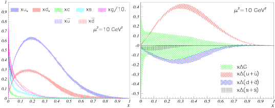
Figure 7: Left: Unpolarized PDFs as function of $x$ for the proton from NNPDF [82, 83]. The valence quarks are denoted $u_{v}$ and $d_{v}$, with $q_{v}(x)=q(x)-\bar{q}(x)$ normalized to the valence content of the proton: $\int_{0}^{1}u_{v}(x)=2$ and $\int_{0}^{1}dxd_{v}(x)=1$. The gluon distribution $g$ is divided by 10 on the figure. Right: Polarized PDFs for the proton. The $\mu^{2}$ values refer to scale at which the PDFs are calculated.

These distributions can be extracted from inclusive DIS (see e.g. Fig. 7). The gluon distribution, also shown in Fig. 7, can be inferred from sum rules and global fits of the DIS data. However, the identification of the specific contribution of quark and gluon OAM to the nucleon spin (Fig. 8) is beyond the parton model analysis. Note that Eq. (25) imposes the constraint $\left|\Delta q_{i}(x)\right|\leq q_{i}(x)$, which together with Eqs. (21) and (23) yields the positivity constraint $\left|g_{1}\right|\leq F_{1}$.

Eqs. (21) and (23) are derived assuming that there is no interference of amplitudes for the lepton scattering at high momentum transfer on one type of quark or another; the final states in the parton model are distinguishable and depend on which quark participates in the scattering and is ejected from the nucleon target; likewise, the derivation of Eqs. (21) and (23) assumes that quantum-mechanical coherence is not possible for different quark scattering amplitudes since the quarks are assumed to be quasi-free. Such interference and coherence effects can arise at lower momentum transfer where quarks can coalesce into specific hadrons and thus participate together in the scattering amplitude. In such a case, the specific quark which scatters cannot be identified as the struck quark. This resonance regime is discussed in Sections 3.2 and 3.3.

The parton model naturally predicts 1) Bjorken scaling: the structure functions depend only on $x=x_{Bj}$; 2) the Callan-Gross relation [84], $F_{2}=2xF_{1}$, reflecting the spin-$1/2$ nature of quarks; i.e., $F_{L}=0$ (no absorption of longitudinal photons in DIS due to helicity conservation); 3) the interpretation of $x_{Bj}$ as the momentum fraction carried by the struck quark in the IMF [34], or equivalently, the quarks’ LF momentum fraction $x=k^{+}/P^{+}$; and 4) a probabilistic interpretation of the structure functions: they are the square of the parton wave functions and can be constructed from individual quark distributions and polarizations in momentum space. The parton model interpretations of $x_{Bj}$ and of structure functions is only valid in the DIS limit and at LO in $\alpha_{s}$. For example, unpolarized PDFs extracted at NLO may be negative [82, 85], see also [86].

In the parton model, only two structure functions are needed to describe the nucleon. The vanishing of $g_{2}$ in the parton model does not mean it is zero in pQCD. In fact, pQCD predicts a non-zero value for $g_{2}$, see Eq. (60). The structure function $g_{2}$ appears when $Q^{2}$ is finite due to 1) quark interactions, and 2) transverse momenta and spins (see e.g., [15]). It also should be noted that the parton model cannot account for DDIS events $\ell p\to\ell^{\prime}pX$, where the proton remains intact in the final state. Such events contribute to roughly 10% of the total DIS rate.

DIS experiments are typically performed at beam energies for which at most the three or four lightest quark flavors can appear in the final state. Thus, for the proton and the neutron, with three active quark flavors:

$$\vspace{-0.3cm}F_{1}^{p}(x) = \frac{1}{2}\bigg{(}\frac{4}{9}\big{(}u(x)+\overline{u}(x)\big{)}+\frac{1}{9}\big{(}d(x)+\overline{d}(x)\big{)}+\frac{1}{9}\big{(}s(x)+\overline{s}(x)\big{)}\bigg{)},$$

$$\vspace{-0.2cm}g_{1}^{p}(x) = \frac{1}{2}\bigg{(}\frac{4}{9}\big{(}\Delta u(x)+\Delta\overline{u}(x)\big{)}+\frac{1}{9}\big{(}\Delta d(x)+\Delta\overline{d}(x)\big{)}+\frac{1}{9}\big{(}\Delta s(x)+\Delta\overline{s}(x)\big{)}\bigg{)},$$

$$\vspace{-0.1cm}F_{1}^{n}(x) = \frac{1}{2}\bigg{(}\frac{1}{9}\big{(}u(x)+\overline{u}(x)\big{)}+\frac{4}{9}\big{(}d(x)+\overline{d}(x)\big{)}+\frac{1}{9}\big{(}s(x)+\overline{s}(x)\big{)}\bigg{)},$$

$$\vspace{-0.0cm}g_{1}^{n}(x) = \frac{1}{2}\bigg{(}\frac{1}{9}\big{(}\Delta u(x)+\Delta\overline{u}(x)\big{)}+\frac{4}{9}\big{(}\Delta d(x)+\Delta\overline{d}(x)\big{)}+\frac{1}{9}\big{(}\Delta s(x)+\Delta\overline{s}(x)\big{)}\bigg{)},$$

where the PDFs $q(x),~{}\overline{q}(x),~{}\Delta q(x)$, and $\Delta\overline{q}(x)$ correspond to the longitudinal light-front momentum fraction distributions of the quarks inside the nucleon. This analysis assumes SU(2)_f charge symmetry, which typically is believed to hold at the 1% level [87, 88].

In the Bjorken limit, this description provides spin information in terms of $x$ (or $x$ and $Q^{2}$ at lower energies, as discussed below). The spatial spin distribution is also accessible, via the nucleon axial form factors. This is analogous to the fact that the nucleon’s electric charge and current distributions are accessible through the electromagnetic form factors measured in elastic lepton-nucleon scattering (see Sec. 3.3). Form factors and particle distributions functions are linked by GPDs and Wigner Functions, which correlate both the spatial and longitudinal momentum information [89], including that of OAM [90].

3.1.9 Perturbative QCD at finite $Q^{2}$

In pQCD, the struck quarks in DIS can radiate gluons; the simplicity of Bjorken scaling is then broken by computable logarithmic corrections. The lowest-order $\alpha_{s}$ corrections arise from 1) vertex correction, where a gluon links the incoming and outgoing quark lines; 2) gluon bremsstrahlung on either the incoming and outgoing quark lines; 3) $q$-$\overline{q}$ pair creation or annihilation. This latter leads to the axial anomaly and makes gluons to contribute to the nucleon spin (see Sec. 5.5). These corrections introduce a power of $\alpha_{s}$ at each order, which leads to logarithmic dependence in $Q^{2}$, corresponding to the behavior of the strong coupling $\alpha_{s}(Q^{2})$ at high $Q^{2}$ [91].

Amplitude calculations, including gluon radiation, exist up to next-to-next-to leading order (NNLO) in $\alpha_{s}$ [92]. In some particular cases, calculations or assessments exist up to fourth order e.g., for the Bjorken sum rule, see Section 5.5. These gluonic corrections are similar to the effects derived from photon emissions (radiative corrections) in QED; they are therefore called pQCD radiative corrections. As in QED, canceling infrared and ultraviolet divergences appear and calculations must be regularized and then renormalized. Dimensional regularization is often used for pQCD (minimal subtraction scheme, $\overline{MS}$) [93], although several other schemes are also commonly used. The pQCD radiative corrections are described to first approximation by the DGLAP evolution equations [56]. This formalism correctly predicts the $Q^{2}$-dependence of structure functions in DIS. The pQCD radiative corrections are renormalization scheme-independent at any order if one applies the BLM/PMC [94, 95] scale-setting procedure.

The small-$x_{Bj}$ power-law Regge behavior of structure functions can be related to the exchange of the Pomeron trajectory using the BFKL equations [57]. Similarly the $t$-channel exchange of the isospin $I=1$ Reggeon trajectory with $\alpha_{R}=1/2$ in DVCS can explain the observed behavior $F_{2p}(x_{Bj},Q^{2})-F_{2n}(x_{Bj},Q^{2})\propto\sqrt{x_{Bj}}$, as shown by Kuti and Weisskopf [96]. This small-$x$ Regge behavior is incorporated in the LFHQCD structure for the $t$-vector meson exchange [97]. A general discussion of the application of Regge dynamics to DIS structure functions is given in Ref. [98]. The evolution of $g_{1}(x_{Bj},Q^{2}$) at low-$x_{Bj}$ has been investigated by Kirschner and Lipatov, and Blumlein and Vogt [99], by Bartels, Ermolaev and Ryskin [100]; and more recently by Kovchegov, Pitonyak and Sievert [101]; See [10] for a summary of small-$x_{Bj}$ behavior of the PDFs. The distribution and evolution at low-$x_{Bj}$ of the gluon spin contributions $\Delta g(x_{Bj})$ and $\mbox{L}_{g}(x_{Bj})$ is discussed in [102], with the suggestion that in this domain, $\mbox{L}_{g}(x_{Bj})\approx-\Delta g(x_{Bj})$. In addition to structure functions, the evolution of the distribution amplitudes in $\ln(Q^{2})$ defined from the valence LF Fock state is also known and given by the ERBL equations [58].

Although the evolution of the $g_{1}$ structure function is known to NNLO [103], we will focus here on the leading order (LO) analysis in order to demonstrate the general formalism. At leading-twist one finds

$$\vspace{-0.3cm}g_{1}(x_{Bj},Q^{2})=\frac{1}{2}\sum_{i}e_{i}^{2}\Delta q_{i}(x_{Bj},Q^{2}),$$ (26)

where the polarized quark distribution functions $\Delta q$ obey the evolution equation

$$\vspace{-0.3cm}\frac{\partial\Delta q_{i}(x,t)}{\partial t}=\frac{\alpha_{s}(t)}{2\pi}\int_{x}^{1}\frac{dy}{y}\left[\Delta q_{i}(y,t)P_{qq}\left(\frac{x}{y}\right)+\Delta g(y,t)P_{qg}\left(\frac{x}{y}\right)\right],$$ (27)

with $t=\ln(Q^{2}/\mu^{2})$. Likewise, the evolution equation for the polarized gluon distribution function $\Delta g$ is

$$\vspace{-0.3cm}\frac{\partial\Delta g(x,t)}{\partial t}=\frac{\alpha_{s}(t)}{2\pi}\int_{x}^{1}\frac{dy}{y}\bigg{[}\sum_{i=1}^{2f}\Delta q_{i}(y,t)P_{gq}\left(\frac{x}{y}\right)+\Delta g(y,t)P_{gg}\left(\frac{x}{y}\right)\bigg{]}.$$ (28)

At LO the splitting functions $P_{\alpha\beta}$ appearing in Eqs. (27) and (28) are given by

$$\vspace{-0.3cm}P_{qq}(z) = \frac{4}{3}\frac{1+z^{2}}{1-z}+2\delta(z-1),$$

$$P_{qg}(z) = \frac{1}{2}\big{(}z^{2}-(1-z)^{2}\big{)},$$

$$P_{gq}(z) = \frac{4}{3}\frac{1-(1-z)^{2}}{z},$$

$$P_{gg}(z) = 3\bigg{[}\big{(}1+z^{4}\big{)}\bigg{(}\frac{1}{z}+\frac{1}{1+z}\bigg{)}-\frac{(1-z)^{3}}{z}\bigg{]}+\bigg{[}\frac{11}{2}-\frac{f}{3}\bigg{]}\delta(z-1).$$

These functions are related to Wilson coefficients defined in the operator product expansion (OPE), see Section 4.1. They can be interpreted as the probability that:

$P_{qq}$: a quark emits a gluon and retains $z=x_{Bj}/y$ of its initial momentum;

$P_{qg}$: a gluon splits into $q$-$\overline{q}$, with the quark having a fraction $z$ of the gluon momentum;

$P_{gq}$: a quark emits a gluon with a fraction $z$ of the initial quark momentum;

$P_{gg}$: a gluon splits in two gluons, with one having the fraction $z$ of the initial momentum.

The presence of $P_{qg}$ allows inclusive polarized DIS to access the polarized gluon distribution $\Delta g(x_{Bj},Q^{2})$, and thus its moment $\Delta G\equiv\int_{0}^{1}\Delta g~{}dx$, albeit with limited accuracy. The evolution of $g_{2}$ at LO in $\alpha_{s}$ is obtained from the above equations applied to the Wandzura-Wilczek relation, Eq. (60).

In general, pQCD can predict $Q^{2}$-dependence, but not the $x_{Bj}$- dependence of the parton distributions which is derived from nonperturbative dynamics (see Section 3.1). The high-$x_{Bj}$ domain is an exception (see Section 6.3). The intuitive DGLAP results are recovered more formally using the OPE, see Section 4.1.

3.1.10 The nucleon spin sum rule and the “spin crisis”

The success of modeling the nucleon with quasi-free valence quarks and with constituent quark models (see Section 3.2.1) suggests that only quarks contribute to the nucleon spin:

$$\vspace{-0.2cm}J=\frac{1}{2}\Delta\Sigma+\mbox{L}_{q}=\frac{1}{2},$$ (29)

where $\Delta\Sigma$ is the quark spin contribution to the nucleon spin $J$;

$$\vspace{-0.3cm}\Delta\Sigma=\sum_{q}\int_{0}^{1}dx\,\Delta q(x),$$ (30)

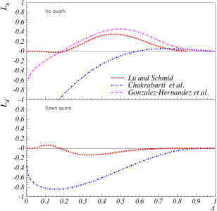
Figure 8: Models predictions for the quark kinematical OAM $L_{z}$, from Refs. [104] (dot-dashed line), [52] (dots), and [105] (dashes).

and $\mbox{L}_{q}$ is the quark OAM contribution. Extracted polarized PDFs and modeled quark OAM distributions are shown in Figs. 7 and 8. It should be emphasized that the existence of the proton’s anomalous magnetic moment requires nonzero quark OAM [63]. For instance, in the Skyrme model, chiral symmetry implies a dominant nonperturbative contribution to the proton spin from quark OAM [106]. It is interesting to quote the conclusion from Ref.  [107]: “Nearly 40% of the angular momentum of a polarized proton arises from the orbital motion of its constituents. In the geometrical picture of hadron structure, this implies that a polarized proton possesses a significant amount of rotation contribution to $S_{z}$ and $\mbox{L}_{z}$ comes from the valence quarks.” (emphasis by the author). QCD radiative effects introduce corrections to the spin dynamics from gluon emission and absorption which evolve in $\ln Q^{2}$. It was generally expected that the radiated gluons would contribute to the nucleon spin, but only as a small correction (beside their effect of introducing a $Q^{2}$-dependence to the different contributions to the nucleon spin). The speculation that polarized gluons contribute significantly to nucleon spin, whereas their sources – the quarks – do not, is unintuitive, although it is a scenario that was (and still is by some) considered (see e.g. the bottom left panel of Fig. 18 on page 18). A small contribution to the nucleon spin from gluons would also imply a small role of the sea quarks, so that $\Delta\Sigma$ and the quark OAM would then be understood as coming mostly from valence quarks. In this framework, it was determined that the quark OAM contributes to about 20% [107, 108] based on the values for $F$ and $D$, the weak hyperon decay constants (see Section 5.5), SU(3)_f flavor symmetry and $\Delta s=0$ [109, 110, 111]. This prediction was made in 1974 and predates the first spin structure measurements by SLAC E80 [112], E130 [113] and CERN EMC [114].

The origin of the quark OAM was later understood as due to relativistic kinematics [110, 111], whereas $\Delta\Sigma$ comes from the quark axial currents (see discussion below Eq. (2)). For a nonrelativistic quark, the lower component of the Dirac spinor is negligible; only the upper component contributes to the axial current. In hadrons, however, quarks are confined in a small volume and are thus relativistic. The lower component, which is in a $p$-wave, with its spin anti-aligned to that of the nucleon, contributes and reduces $\Delta\Sigma$. At that time, it seemed reasonable to neglect gluons, thus predicting a nonzero contribution to $J$ from the quark OAM. The result was the initial expectation $\Delta\Sigma\approx$ 0.65 and thus the quark OAM was about 18%. Since this review is also concerned with spin composition of the nucleon at low energy, it is interesting to remark that a large quark OAM contribution would essentially be a confinement effect.

The first high-energy measurements of $g_{1}(x_{Bj},Q^{2})$ was performed at SLAC in the E80 [112] and E130 [113] experiments. The data covered a limited $x_{Bj}$ range and agreed with the naive model described above. However, the later EMC experiment at CERN [114] measured $g_{1}(x_{Bj},Q^{2})$ over a range of $x_{Bj}$ sufficiently large to evaluate moments. It showed the conclusions based on the SLAC measurements to be incorrect. The EMC measurement suggests instead that $\Delta\Sigma\approx 0$, with large uncertainty. This contradiction with the naive model became known as the “spin crisis”.

Although more recent measurements at COMPASS, HERMES and Jlab are consistent with a value of $\Delta\Sigma\approx 0.3$, the EMC indication still stands that gluons and/or gluon and quark OAM are more important than had been foreseen; see e.g., Ref. [115]. Since gluons are possibly important, $J$ must obey the total angular momentum conservation law known as the “nucleon spin sum rule”

$$\vspace{-0.3cm}J=\frac{1}{2}\Delta\Sigma(Q^{2})+\mbox{L}_{q}(Q^{2})+\Delta G(Q^{2})+\mbox{L}_{g}(Q^{2})=\frac{1}{2},$$ (31)

at any scale $Q$. The gluon spin $\Delta G$ represents with $\mbox{L}_{g}$ a single term, $\Delta G+\mbox{L}_{g}$, since the individual $\Delta G$ and $\mbox{L}_{g}$ contributions are not separately gauge-invariant. (This is discussed in more detail in the next section.) The terms in Eq. (31) are obtained by utilizing LF-quantization or the IMF and the LC gauge, writing the hadronic angular momentum tensor in terms of the quark and gluon fields [110]. In the gauge and frame-dependent partonic formulation, in which $\Delta G$ and $\mbox{L}_{g}$ can be separated, Eq. (31) is referred to as the Jaffe-Manohar decomposition. An alternative formulation is given by Ji’s decomposition. It is gauge/frame independent, but its partonic interpretation is not as direct as for the Jaffe-Manohar decomposition [116].

The quantities in Eq. (31) are integrated over $x_{Bj}$. They have been determined at a moderate value of $Q^{2}$, typically 3 or 5 GeV². Eq. (31) does not separate sea and valence quark contributions. Although DIS observables do not distinguish them, separating them is an important task. In fact, recent data and theoretical developments indicate that the valence quarks are dominant contributors to $\Delta\Sigma$. We also note that the strange and anti-strange sea quarks can contribute differently to the nucleon spin [117]. Finally, a separate analysis of spin-parallel and antiparallel PDFs is clearly valuable since they have different nonperturbative inputs.

A transverse spin sum rule similar to Eq. (31) has also been derived [118, 119]. Likewise, transverse versions of the Ji sum rule (see next section) exist [120, 121], together with debates on which version is correct. Transverse spin not being the focus of this review, we will not discuss this issue further.

The $Q^{2}$-evolution of quark and gluon spins discussed in Section 3.1.9 provides the $Q^{2}$-evolution of $\Delta\Sigma$ and $\Delta G$. The evolution equations are known to at least NNLO and are discussed in Section 5.5. The evolution of the quark and gluon OAM is known to NLO [122, 123, 124, 125, 126]. The evolution of the nucleon spin sum rule components at LO is given in Ref. [122]:

$$\Delta\Sigma(Q^{2})=\mbox{constant},\vspace{-0.1cm}$$

$$\mbox{L}_{q}(Q^{2})=\frac{-\Delta\Sigma(Q^{2})}{2}+\frac{3n_{f}}{32+6n_{f}}+\bigg{(}\mbox{L}_{q}(Q_{0}^{2})+\frac{-\Delta\Sigma(Q^{2}_{0})}{2}-\frac{3n_{f}}{32+6n_{f}}\bigg{)}(t/t_{0})^{-\frac{32+6n_{f}}{9\beta_{0}}},$$

$$\Delta G(Q^{2})=\frac{-4\Delta\Sigma(Q^{2})}{\beta_{0}}+\bigg{(}\Delta G(Q_{0}^{2})+\frac{4\Delta\Sigma(Q^{2}_{0})}{\beta_{0}}\bigg{)}\frac{t}{t_{0}},$$

$$\vspace{-0.1cm}\mbox{L}_{g}(Q^{2})=-\Delta G(Q^{2})+\frac{8}{16+3n_{f}}+\bigg{(}\mbox{L}_{q}(Q_{0}^{2})+\Delta G(Q_{0}^{2})-\frac{8}{16+3n_{f}}\bigg{)}(t/t_{0})^{-\frac{32+6n_{f}}{9\beta_{0}}}$$ (32)

with $t=\ln(Q^{2}/\Lambda_{s}^{2})$ and $Q_{0}^{2}$ the starting scale of the evolution. The QCD $\beta$-series is defined here such that $\beta_{0}=11-\frac{2}{3}n_{f}$. The NLO equations can be found in Ref. [126].

3.1.11 Definitions of the spin sum rule components

Values for the components of Eq. (31) obtained from experiments, Lattice Gauge Theory or models are given in Section 6.11 and in the Appendix. It is important to recall that these values are convention-dependent for several reasons. One is that the axial anomaly shifts contributions between $\Delta\Sigma$ and $\Delta G$, depending on the choice of renormalization scheme, even at arbitrary high $Q^{2}$ (see Section 5.5). This effect was suggested as a cause for the smallness of $\Delta\Sigma$ compared to the naive quark model expectation: a large value $\Delta G\approx 2.5$ would increase the measured $\Delta\Sigma$ to about 0.65. Such large value of $\Delta G$ is nowadays excluded. Furthermore, it is unintuitive to use a specific renormalization scheme in which the axial anomaly contributes, to match quark models that do not need renormalization. Another reason is that the definitions of $\Delta G$, $\mbox{L}_{q}$, $\mbox{L}_{g}$ are also conventional. This was known before the spin crisis [110] but the discussion on what the best operators are has been renewed by the derivation of the Ji sum rule [127]:

$$\vspace{-0.3cm}J_{q,g}=\frac{1}{2}\int_{-1}^{1}x\big{[}E_{q,g}(x,0,0)+H_{q,g}(x,0,0)\big{]}dx,$$ (33)

with $\sum_{q}J^{q}+J^{g}=\frac{1}{2}$ being frame and gauge invariant and $J_{q,g}$ and the GPDs $E_{q,g}$ and $H_{q,g}$ stand either for quarks or gluons. For quarks, $J_{q}\equiv\Delta\Sigma/2+\mbox{L}_{q}$. For gluons, $J_{g}$ cannot be separated into spin and OAM parts in a frame or gauge invariant way. (However, it can be separated in the IMF, with an additional “potential” angular momentum term [67].)

Importantly, the Ji sum rule provides a model-independent access to $\mbox{L}_{q}$, whose measurability had been until then uncertain. Except for Lattice Gauge Theory (see Section 4.2.2) the theoretical assessments of the quark OAM are model-dependent. We mentioned the relativistic quark model that predicted about 20% even before the occurrence of the spin crisis. More recently, investigation within an unquenched quark model suggested that the unpolarized sea asymmetry $\overline{u}-\overline{d}$ is proportional to the nucleon OAM:

$$\vspace{-0.3cm}\mbox{L}(Q^{2})\equiv\mbox{L}_{q}(Q^{2})+\mbox{L}_{g}(Q^{2})\propto\big{(}\overline{u}(Q^{2})-\overline{d}(Q^{2})\big{)},$$ (34)

where $\overline{q}(Q^{2})=\int_{0}^{1}\overline{q}(x,Q^{2})dx$. The non-zero $\overline{u}-\overline{d}$ distribution is well measured [128] and causes the violation of the Gottfried sum rule [129, 130]. The initial derivation of Eq. (34) by Garvey [131] indicates a strict equality, $L=(\overline{u}-\overline{d})=0.147\pm 0.027$, while a derivation in a chiral quark model [132] suggests $L=1.5(\overline{u}-\overline{d})=0.221\pm 0.041$. The lack of precise polarized PDFs at low-$x_{Bj}$ does not allow yet to verify this remarkable prediction [133]. Another quark OAM prediction is from LFHQCD: $\mbox{L}_{q}(Q^{2}\leq Q_{0}^{2})=1$ in the strong regime of QCD, evolving to $\mbox{L}_{q}=0.35\pm 0.05$ at $Q^{2}=5$ GeV², see Section 4.4.

Beside Eq. (33) and possibly Eq. (34), the quark OAM can also be accessed from the two-parton twist-3 GPD $G_{2}$ [66]:

$$\vspace{-0.2cm}\mbox{L}_{q}=-\int\ G^{q}_{2}(x,0,0)dx,$$ (35)

or generalized TMD (GTMD) [44, 53, 134]. TMD allow to infer $\mbox{L}_{q}$ model-dependently [49].

Jaffe and Manohar set the original convention to define the angular momenta [110]. They expressed Eq. (31) using the canonical angular momentum and momentum tensors. This choice is natural since it follows from Noether’s theorem [119]. For angular momenta, the relevant symmetry is the rotational invariance of QCD’s Lagrangian. The ensuing conserved quantity (i.e., that commutes with the Hamiltonian) is the generator of the rotations. This definition provides the four angular momenta of the longitudinal spin sum rule, Eq. (31). A similar transverse spin sum rule was also derived [118, 119]. A caveat of the canonical definition is that in Eq. (31), only $J$ and $\Delta\Sigma$ are gauge invariant, i.e., are measurable. In the light-cone gauge, however, the gluon spin term coincides with the measured observable $\Delta G$. (This is true also in the $A^{0}=0$ gauge [15].) The fundamental reason for the gauge dependence of the other components of Eq. (31) is their derivation in the IMF.

What triggered the re-inspection of the Jaffe-Manohar decomposition and subsequent discussions was that Ji proposed another decomposition using the Belinfante-Rosenfeld energy-momentum tensor [135], which lead to the Ji sum rule [127], Eq. (33). The Belinfante-Rosenfeld tensor originates from General Relativity in which the canonical momentum tensor is modified so that it becomes symmetric and conserved (commuting with the Hamiltonian): in a world without angular momentum, the canonical momentum tensor would be symmetric. However, adding spins breaks its symmetry. An appropriate combination of canonical momentum tensor and spin tensor yields the Belinfante-Rosenfeld tensor, which is symmetric and thus natural for General Relativity where it identifies to its field source (i.e. the Hilbert tensor). The advantages of such definition are 1) its naturalness even in presence of spin; 2) that it leads to a longitudinal spin sun rule in which all individual terms are gauge invariant; and 3) that there is a known method to measure $\mbox{L}_{q}$ (Eq. (33)), or to compute it using Lattice Gauge Theory (see Section 4.2.2). Its caveat is that the nucleon spin decomposition contains only three terms: $\Delta\Sigma$, $\mbox{L}_{q}$ and a global gluon term, thus without a clear interpretation of the experimentally measured $\Delta G$. While $\Delta\Sigma$ in the Ji and Jaffe-Manohar decompositions are identical, the $\mbox{L}_{q}$ terms are different. That several definitions of $\mbox{L}_{q}$ are possible comes from gauge invariance. To satisfy it, quarks do not suffice; gluons must be included, which allows for choices in the separation of $\mbox{L}_{q}$ and $\mbox{L}_{g}$ [136, 137]. The general physical meaning of $\mbox{L}_{q}$ is that it is the torque acting on a quark during the polarized DIS process [39, 138]: Ji’s $\mbox{L}_{q}$ is the OAM before the probing photon is absorbed by the quark, while the Jaffe-Manohar $\mbox{L}_{q}$ is the OAM after the photon absorption, with the absorbing quark kicked out to infinity. These two definitions of $\mbox{L}_{q}$ have been investigated with several models, e.g., [137, 139], whose results are shown in Section 6.11.2.

Other definitions of angular moments and gluon fields have been proposed to eliminate the gauge-dependence problem [140], leading to a spin decomposition Eq. (31) with four gauge-invariant terms. The complication is that the corresponding operators use non-local fields, viz fields depending on several space-time variables or, more generally, a field $A$ for which $A(x)\neq e^{-ipx}A(0)e^{ipx}$.

Recent reviews on angular momentum definition and separation are given in Ref. [136]. It remains to be added that in practice, to obtain $\mbox{L}_{q}$ in a leading-twist (twist 2) analysis, $\Delta\Sigma/2$ must be subtracted, see Eq. (33). Thus, since $\Delta\Sigma$ is renormalization scheme dependent due to the axial anomaly, $\mbox{ L}_{q}$ is too (but not their sum $J_{q}$). A higher-twist analysis of the nucleon spin sum rule allows to separate quark and gluon spin contributions (twist 2 PDFs/GPDs) from their OAM (twist 3 GPD $G_{2}$) [66, 67, 121, 134, 141]. It is expected that OAM are twist-3 quantities since they involve the parton’s transverse motions. However, the quark OAM, as defined in Eq. (33) can be related to twist-2 GPDs. Beside GPDs, OAM can also be accessed with GTMDs [49, 53, 68, 142]. It is now traditional to call the Jaffe-Manohar OAM the canonical expression and denote it by $l_{z}$, the Ji OAM is called kinematical and denoted by $L_{z}$. We will use this convention for the rest of the review.

In summary, the components of Eq. (31) are scheme and definition (or gauge) dependent. Thus, when discussing the origin of the nucleon spin, schemes and definitions must be specified. This is not a setback since, as emphasized in the preamble, the main object of spin physics is not to provide the pie chart of the nucleon spin but rather to use it to verify QCD’s consistency and understand complex mechanisms involving it, e.g., confinement. That can be done consistently in fixed schemes and definitions. This leads us to the next section where such complex mechanisms start to arise.

3.2 The resonance region

At smaller values of $W$ and $Q^{2}$, namely below the DIS scaling region, the nucleon reacts increasingly coherently to the photon until it eventually responds fully rigidly. Before reaching this elastic reaction on the nucleon ground state, scattering may excite nucleon states of higher masses where no specific quark can unambiguously be said to have been struck, thus causing interference and coherence effects. One thus leaves the DIS domain to enter the resonance region characterized by bumps in the scattering cross-section, see Fig. 3. These higher-spin resonances are OAM and radially excited nucleon states. They then decay by meson or/and photon emission and can be classified into two groups: isospin 1/2 (N^∗ resonances) and isospin 3/2 ($\Delta^{*}$ resonances).

The resonance domain is important for this review since it covers the transition from pQCD to nonperturbative QCD. It also illustrates how spin information can illuminate QCD phenomena. Since the resonances are numerous, overlapping and differ in origin, spin degrees of freedom are needed to identify and characterize them. Modern hadron spectroscopy experiments typically involve polarized beams and targets. However, inclusive reactions are ill suited to disentangle resonances: final hadronic states must be partly or fully identified. Thus, we will cover this extensive subject only superficially.

The nomenclature classifying nucleon resonances originates from $\pi N$ scattering. Resonances are labelled by L${}_{2I~{}2J}$, where L is the OAM in the $\pi N$ channel (not the hadron wavefunction OAM), $I$=1/2 or 3/2 is the isospin, and $J$ is the total angular momentum. L is labeled by S (for L=0), P (L=1), D (L=2) or F (L=3). An important tool to classify resonances and predict their masses is the constituent quark model, which is discussed next. Lattice gauge theory (Section 4.2) is now the main technique to predict and characterize resonances, with the advantage of being a first-principle QCD approach. Another successful approach based on QCD’s basic principles and symmetries is LF Holographic QCD (Section 4.4), an effective theory which uses the gauge/gravity duality on the LF, rather than ordinary spacetime, to captures essential aspects of QCD dynamics in its nonperturbative domain.

3.2.1 Constituent quark models

The basic classification of the hadron mass spectra was motivated by the development of constituent quark models obeying an $SU(6)\supset SU(3)_{flavor}\otimes SU(2)_{spin}$ internal symmetry [109, 143]. Baryons are modeled as composites of three constituent quarks of mass $M/3$ (modulo binding energy corrections which depend on the specific model) which provides the $J^{PC}$ quantum numbers. The constituent quark model predates QCD but is now interpreted and developed in its framework. Constituent quarks differ from valence quarks – which also determine the correct quantum numbers of hadrons – in that they are not physical (their mass is larger) and are understood as valence quarks dressed by virtual partons. The large constituent quark masses explicitly break both the conformal and chiral symmetries that are nearly exact for QCD at the classical level; see Sections 4.3. Constituent quarks are assumed to be bound at LO by phenomenological potentials such as the Cornell potential [144], an approach which was interpreted after the advent of QCD as gluonic flux tubes acting between quarks. The LO spin-independent potential is supplemented by a spin-dependent potential, e.g., by adding exchange of mesons [145], instantons or by including the interaction of a spin-1 gluon exchanged between the quarks (“hyperfine correction” [146, 147]). “Constituent gluons” have also been used to characterize mesons that may exhibit explicit gluonic degrees of freedom (“hybrid mesons”). The constituent quark models, which have been built to explain hadron mass spectroscopy, can reproduce it well. In particular, they historically lead to the discovery of color charge. Of particular interest to this review, such an approach can also account for baryon magnetic moments which can be distinguished from the constituent quark pointlike (i.e., Dirac) magnetic moments. Another feature of these models relevant to this review is that the physical mechanisms that account for hyperfine corrections are also needed to explain polarized PDFs at large-$x_{Bj}$, see Section 6.3.1. Hyperfine corrections can effectively transfer some of the quark spin contribution to quark OAM [149], consistent with the need for non-zero quark OAM in order to describe the PDFs within pQCD [150].

In non-relativistic constituent quark models, the quark OAM is zero and there are no gluons: the nucleon spin comes from the quark spins. SU(6) symmetry and requiring that the non-color part of the proton wavefunction is symmetric yield [146, 151]:

$$\vspace{-0.3cm}\left|p\uparrow\right\rangle=\frac{1}{\sqrt{2}}\left|u\uparrow(ud)_{\mathbf{s}=0,s=0}\right\rangle+\frac{1}{\sqrt{18}}\left|u\uparrow(ud)_{\mathbf{s}=1,s=0}\right\rangle-$$ (36)

$$\frac{1}{3}\left(\left|u\downarrow(ud)_{\mathbf{s}=1,s=1}\right\rangle-\left|d\uparrow(uu)_{\mathbf{s}=1,s=0}\right\rangle+\sqrt{2}\left|d\downarrow(uu)_{\mathbf{s}=1,s=1}\right\rangle\right),$$

where the arrows indicate the projection of the 1/2 spins along the quantization axis, while the subscripts $\mathbf{s}$ and $s$ denote the total and projected spins of the diquark system, respectively. The neutron wavefunction is obtained from the proton wavefunction via isospin $u\leftrightarrow d$ interchange. The spectroscopy of the excited states varies between models, depending in detail on the choice of the quark potential.

As mentioned in Section 3.1.10, the disagreement between the EMC experimental results [114], and the naive $\Delta\Sigma=1$ expectation from the simplest constituent quark models has led to the “spin crisis”. Myhrer, Bass, and Thomas have interpreted the “spin crisis” in the constituent quark model framework as a pion cloud effect [115, 152], which together with relativistic corrections and one-gluon exchange, can transfer part of $\Delta\Sigma$ to the quark OAM (mostly to $l^{u}_{q}$) [153]. Once these corrections have been applied, the constituent quark picture – which has had success in describing other aspects of the strong force – also becomes consistent with the spin structure data. Relativistic effects, one-gluon exchange and the pion cloud reduce the naive $\Delta\Sigma=1$ expectation by 35%, 25% and 20%, respectively. The quark spin contribution is transferred to quark OAM, resulting in $\Delta\Sigma/2\approx 0.2$ and $l_{q}\approx+0.3$. These predictions apply at the low momentum scale where DGLAP evolution starts, estimated to be $Q_{0}^{2}\approx 0.16$ GeV² [154], which could be relevant to the constituent quark degrees of freedom. Evolving these numbers from $Q_{0}^{2}$ to the typical DIS scale of 4 GeV² using Eqs. (32) decreases the quark OAM to 0 ($l_{q}^{d}\approx-l_{q}^{u}\approx 0.1$), transferring it to $\Delta G+\mbox{L}_{g}$. Thus, the Myhrer-Bass-Thomas model yields $\Delta\Sigma/2\approx 0.18$, $l_{q}\approx 0$ and $\Delta G+\mbox{L}_{g}\approx 0.32$, with strange and heavier quarks not directly contributing to $J$.

This result is not supported by those of Refs. [126, 155] which assessed the value of $L_{q}$ at low scales by evolving down large scale LGT estimates of the spin sum rule components. A cause of the disagreement might be that Refs. [126, 155] use LGT input, i.e., with the quark OAM kinematical definition, while it is unclear which definition applies to the quark OAM in constituent quark models, such as that used in Refs. [154]. Furthermore, the high scale $L_{q}$ input of Refs. [126, 155] stems from early LGT calculations which do not include disconnected diagrams. Those are now known to contribute importantly to the quark OAM, which makes the $L_{q}$ input of Refs. [126, 155] questionnable. Finally, the scale evolutions are preformed in [126, 154, 155] at leading twist, which is known to be insufficient for scales below $Q_{0}\approx 1$ GeV [156, 157]. (We remark that some higher-twists are effectively included when a non-perturbative $\alpha_{s}$ is employed). The limitation of these evolutions in the very low scale region characterizing bag models (0.1-0.3 GeV²) is in particular studied in Ref. [126]. The authors improved the cloudy bag model calculation of Ref. [154] by using the gauge-invariant (kinematical) definition of the spin contributions. It yields $Q_{0}^{2}\approx 0.2$ GeV², $\Delta\Sigma/2=0.23\pm 0.01$, $L_{q}=0.53\pm 0.09$ and $\Delta G+\mbox{L}_{g}=-0.26\pm 0.10$. The importance of the pion cloud to $J$ has also been discussed in Refs. [133, 158].

3.2.2 The resonance spectrum of nucleons

The first nucleon excited state is the P₃₃, also called the $\Delta(1232)~{}3/2^{+}$ ($M_{\Delta}$=1232 MeV) in which the three constituent quark spins are aligned while in an S-wave. Thus, the $\Delta(1232)~{}3/2^{+}$ has spin $J=3/2,$ and its isospin is 3/2. The $\Delta(1232)~{}3/2^{+}$ resonance is the only one clearly identifiable in an inclusive reaction spectrum. It has the largest cross-section and thus contributes dominantly to sum rules (Section 5) and moments of spin structure functions at moderate $Q^{2}$. The nucleon-to-$\Delta$ transition is thus, in this SU(6)-based view, a spin (and isospin) flip; i.e., a magnetic dipole transition quantified by the $M_{1+}$ multipole amplitude. Experiments have shown that there is also a small electric quadrupole component $E_{1+}$ ($E_{1+}/M_{1+}<0.01$ at Q${}^{2}=0$) which violates SU(6) isospin-spin symmetry. This effect can be interpreted as the deformation of the $\Delta(1232)~{}3/2^{+}$ charge and current distributions in comparison to a spherical distribution. The nomenclature for multipole longitudinal (also called scalar) amplitudes $S_{l\pm}$, as well as the transverse $E_{l\pm}$ and $M_{l\pm}$ amplitudes is given in Ref. [20]. The small $E_{1+}$ and $S_{1+}$ components are predicted by constituent quark models improved with a $M_{1}$ dipole-type one-gluon exchange (see Section 6.3).

Due to their similar masses and short lifetimes (i.e., large widths in excitation energy $W$), the higher mass resonances overlap, and thus cannot be readily isolated as distinct contributions to inclusive cross-sections. Their contributions can be grouped into four regions whose shapes and mean-$W$ vary with $Q^{2}$, due to the different $Q^{2}$-behavior of the amplitudes of the individual resonances. The second resonance region (the first is the $\Delta(1232)~{}3/2^{+}$) is located at $W\approx 1.5$ GeV and contains the N(1440) $1/2^{+}$ P₁₁ (Roper resonance), the N(1520) $3/2^{-}$ D₁₃ and the N(1535) $1/2^{-}$ S₁₁ which usually dominates over the first two. The third region, at $W\approx 1.7$ GeV, includes the $\Delta$(1600) $3/2^{+}$ P₃₃, N(1680) $5/2^{+}$ F₁₅, N(1710) $1/2^{-}$ P₁₁, N(1720) $3/2^{+}$ P₁₃, $\Delta$(1620) $1/2^{-}$ S₃₁, N(1675) $5/2^{-}$ D₁₅, $\Delta$(1700) $3/2^{-}$ D₃₃, and N(1650) $1/2^{-}$ S₁₁. The fourth region is located around $W\approx 1.9$ GeV and contains the $\Delta$(1905) $5/2^{+}$ F₃₅, $\Delta$(1920) $3/2^{+}$ P₃₃, $\Delta$(1910) $1/2^{+}$ P₃₁, $\Delta$(1930) $5/2^{+}$ D₃₅ and $\Delta$(1950) $7/2^{+}$ F₃₇. Other resonances have been identified beyond $W=2$ GeV [18], but their structure cannot be distinguished in an inclusive experiment not only because of the overlap of their widths, but also because of the dominance of the “non-resonant background” – incoherent scattering similar to DIS at higher $Q^{2}$. Its presence is necessary to satisfy the unitarity of the $S$ matrix in the resonance region.

The DIS cross-section formulae remain valid in the resonance domain. Although the intepretation of structure functions as PDFs cannot be applied, the DIS cross-sections can nevertheless be related to overlaps of LFWFs, as shall be discussed below.

3.2.3 A link between DIS and resonances: hadron-parton duality

Bloom and Gilman observed [159] that the unpolarized structure function $F_{2}(x_{Bj},Q^{2})$ measured in DIS matches $F_{2}(x_{Bj},Q^{2})$ measured in the resonance domain if the resonance peaks are suitably smoothed and if the $Q^{2}$-dependence of $F_{2}$ – due to pQCD radiations and the non-zero nucleon mass – is corrected for. This correspondence is known as hadron-parton duality. It implies that Bjorken scaling, corrected for DGLAP evolution and non-zero mass terms (kinematic twists, see Section 4.1), is effectively valid in the resonance region if the resonant structures can be averaged over. This indicates that the effect of the third source of $Q^{2}$-dependence, the parton correlations (dynamical twists, see Section 4.1), can be neglected. Thus the resonance region can be described in dual languages – either hadronic or partonic [160]. The understanding of hadron-parton duality for spin structure functions has also progressed and is discussed in Section 6.10.

3.3 Elastic and quasi-elastic scatterings

When a leptonic scattering reaction occurs at low energy transfer $\nu={p\cdot q/M}$ and/or low photon virtuality $Q^{2}$, nucleon excited states cannot form. Coherent elastic scattering occurs, leaving the target in its ground state. The transferred momentum is shared by the target’s constituents, the target stays intact and its structure undisrupted. The 4-momentum of the virtual photon is spent entirely as target recoil. The energy transferred is $\nu_{el}=Q^{2}/(2M)$. For a nuclear target, elastic scattering may occur on the nucleus itself or on an individual nucleon. If the nuclear structure is disrupted, the reaction is called quasi-elastic (not to be confused with the “quasi-elastic” scattering of neutrinos, which is charge-exchange elastic scattering; i.e., involving $W^{+/-}$ rather that $Z^{0}$).

For elastic scattering, there is no need for “polarized form factors”: the unpolarized and polarized parts of the cross-section contain the same form factors. This is because in elastic scattering, the final hadronic state is known, from current and angular momentum conservations. Thus, a hadronic current (a vector) can be constructed, which requires two parameters. In contrast, in the inclusive inelastic case, such current cannot be constructed since the final state is by definition undetermined. Only the hadronic tensor can be constructed, which requires four parameters. That the same form factors describe both unpolarized and polarized elastic scattering allowes for accurate form factor measurements [161], which illustrates how spin is used as a complementary tool for exploring nucleon structure.

The elastic reaction is important for doubly-polarized inclusive scattering experiments. Since the same form factors control the unpolarized and polarized elastic cross-sections, the elastic asymmetry is calculable from the well-measured unpolarized elastic scattering. This asymmetry can be used to obtain or check beam and target polarizations. Likewise, the unpolarized elastic cross-section can be used to set or to verify the normalization of the polarized inelastic cross-section. Furthermore, some spin sum rules, e.g., Burkhardt-Cottingham sum rule (see Section 5.4), include the elastic contribution. Such sum rules are valid for nuclei. Therefore, alongside the nucleon, we provide below the formalism of doubly-polarized elastic and quasi-elastic scatterings for the deuteron and ³He nuclei, which are commonly used in doubly-polarized inclusive experiments.

3.3.1 Elastic cross-section

The doubly polarized elastic cross-section is:

$$\vspace{-0.1cm}\frac{d\sigma}{d\Omega}=\frac{\sigma_{Mott}E^{\prime}Z^{2}}{E}\bigg{[}\bigg{(}\frac{Q^{2}}{\overrightarrow{q}^{2}}\bigg{)}^{2}R_{L}(Q^{2},\nu)+\big{(}\tan^{2}(\theta/2)-\frac{1}{2}\frac{Q^{2}}{\overrightarrow{q}^{2}}\big{)}R_{T}(Q^{2},\nu)\pm\Delta(\theta^{*},\phi^{*},E,\theta,Q^{2})\bigg{]},$$ (37)

where $Z$ is the target atomic number and the angles are defined in Fig. 2. $R_{L}$ and $R_{T}$ are the longitudinal and transverse response functions associated with the corresponding polarizations of the virtual photon. The cross-section asymmetry $\Delta$, where $\pm$ refers to the beam helicity sign [162], is:

$$\vspace{-0.3cm}\Delta=-\left(\tan\frac{\theta}{2}\sqrt{\frac{Q^{2}}{\overrightarrow{q}^{2}}+\tan^{2}\frac{\theta}{2}}R_{T^{\prime}}(Q^{2})\cos\theta^{*}-\frac{\sqrt{2}Q^{2}}{\overrightarrow{q}^{2}}\tan\frac{\theta}{2}R_{TL^{\prime}}(Q^{2})\sin\theta^{*}\cos\phi^{*}\right).$$

Cross-sections for the targets used in nucleon spin structure experiments are given below:

Nucleon case

The cross-section for scattering on a longitudinally polarized nucleon is:

$$\frac{d\sigma}{d\Omega} = \sigma_{Mott}\frac{E^{\prime}}{E}\left(W_{2}+2W_{1}\tan^{2}(\theta/2)\right)\times$$

$$\left(1\pm\sqrt{\frac{\tau_{r}W_{1}}{(1+\tau_{r})W_{2}-\tau_{r}W_{1}}}\frac{\frac{2M}{\nu}+\sqrt{\frac{W_{1}}{\tau_{r}\left((1+\tau_{r})W_{2}-\tau_{r}W_{1}\right)}}\frac{2\tau_{r}M}{\nu}+2(1+\tau_{r})\tan^{2}(\theta/2)}{1+\tau_{r}\frac{W_{1}}{\tau_{r}\left((1+\tau_{r})W_{2}-\tau_{r}W_{1}\right)}\left(1+2(1+\tau_{r})\tan^{2}(\theta/2)\right)}\right),$$

with the recoil term $\tau_{r}\equiv Q^{2}/(4M^{2})$. The hadronic current is usually parameterized by the Sachs form factors, $G_{E}(Q^{2})$ and $G_{M}(Q^{2})$, rather than $W_{1}$ and $W_{2}$:

$$\vspace{-0.3cm}W_{1}(Q^{2})=\tau_{r}G_{M}(Q^{2})^{2},\\ \ ~{}~{}~{}~{}~{}W_{2}(Q^{2})=\frac{G_{E}(Q^{2})^{2}+\tau_{r}G_{M}(Q^{2})^{2}}{1+\tau_{r}}.$$

In the nonrelativistic domain the form factors $G_{E}$ and $G_{M}$ can be thought of as Fourier transforms of the nucleon charge and magnetization spatial densities, respectively. A rigorous interpretation in term of LF charge densities is given in Refs. [163] (nucleon) and [164] (deuteron, see next section). The Dirac and Pauli form factors $F_{1}(Q^{2})$ and $F_{2}(Q^{2})$ can also be used (not to be confused with the DIS structure functions in Section 3.1):

$$\vspace{-0.3cm}G_{E}(Q^{2})=F_{1}(Q^{2})-\tau_{r}\kappa_{n}F_{2}(Q^{2}),\\ \ ~{}~{}~{}~{}~{}G_{M}(Q^{2})=F_{1}(Q^{2})+\kappa_{n}F_{2}(Q^{2}),$$

where $\kappa_{n}$ is the nucleon anomalous magnetic moment. The helicity conserving current matrix element generates $F_{1}(Q^{2})$. $F_{2}(Q^{2})$ stems from the helicity-flip matrix element.

LF quantization of QCD provides an interpretation of $F_{1}(Q^{2})$ and $F_{2}(Q^{2})$ which can then be modeled using the structural forms for arbitrary twist inherent to the LFHQCD formalism [165], see Section 4.4. In LF QCD, form factors are obtained from the Drell-Yan-West formula [166, 167] as the overlap of the hadronic LFWFs solutions of LF Hamiltonian $P^{-}$, Eq. (7) [63]. In particular, $F_{2}(Q^{2})$ stems from the overlap of $L=0$ and $L=1$ LFWFs. For a ground state system, the leading-twist of a reaction, that is, its power behavior in $Q^{2}$ (or in the LF impact parameter $\zeta$, see Section 4.1), reflects the leading-twist $\tau$ of the target wavefunction, which is equal to the number of constituents in the LF valence Fock state with zero internal orbital angular momentum. This result is intuitively clear, since in order to keep the target intact after elastic scattering, a number $\tau-1$ of gluons of virtuality $\propto Q^{2}$ must be exchanged between the $\tau$ constituents. For example, at high-$Q^{2}$, all nucleon components are resolved and the twist is $\tau=3$. Higher Fock states including additional $q\overline{q}$, $q\overline{q}q\overline{q}$,…components generated by gluons are responsible for the higher-twists corrections. These constraints are inherent to LFHQCD which can be used to model the LFWFs and thus obtain predictions for the form factors. Alternatively, one can parameterize the general form expected from the twist analysis in terms of weights reflecting the ratio of the higher Fock state probabilities with respect to the leading Fock state wavefunction. These weights provide the probabilities of finding the nucleon in a higher Fock state, computed from the square of the higher Fock state LFWFs. Two parameters suffice to describe the world data for the four spacelike nucleon form factors [165].

Deuteron case

The deuteron is a spin-1 nucleus. Three elastic form factors are necessary to describe doubly polarized elastic cross-sections:

$$\vspace{-0.3cm}\frac{d\sigma}{d\Omega}=\sigma_{M}\frac{E^{\prime}}{E}\big{(}A(Q^{2})+B(Q^{2})\tan^{2}(\theta/2)\big{)}\big{(}1+A^{V}+A^{T}\big{)},$$ (39)

where $A^{V}$ and $A^{T}$, the asymmetries stemming respectively from the vector and tensor polarizations of the deuteron, are

$$\vspace{-0.3cm}A^{V}=\frac{3P_{b}P_{z}}{\sqrt{2}}\bigg{(}\frac{1}{\sqrt{2}}\cos\theta^{*}T_{10}-\sin\theta^{*}T_{11}\bigg{)},$$

where $P_{b}$ is the beam polarization and $P_{z}$ the deuteron vector polarization, $P_{z}=(n_{+}-n_{-})/n_{tot}$. The $n_{i}$ are the populations for the spin values $i$, and $n_{tot}=n_{+}+n_{-}+n_{0}$,

$$\vspace{-0.3cm}A^{T}=\frac{P_{zz}}{\sqrt{2}}\bigg{(}\frac{3\cos^{2}\theta^{*}-1}{2}T_{20}-\sqrt{\frac{3}{2}}\sin(2\theta^{*})\cos\phi^{*}T_{21}+\sqrt{\frac{3}{2}}\sin^{2}\theta^{*}\cos(2\phi^{*})T_{22}\bigg{)},$$

with the deuteron tensor polarization $P_{zz}=(n_{+}+n_{-}-2n_{0})/n_{tot}$.

The seven factors in Eq. (39), $A$, $B$, $T_{10}$, $T_{11}$, $T_{20}$, $T_{21}$ and $T_{22}$, are combinations of three form factors (monopole $G_{C}$, quadrupole $G_{Q}$ and magnetic dipole $G_{M}$):

$$\vspace{-0.3cm}A = G_{C}^{2}+\frac{8}{9}\tau_{r}^{2}G_{Q}^{2}+\frac{2}{3}\tau_{r}G_{M}^{2},$$ (40)

$$\ B = \frac{4}{3}\tau_{r}(1+\tau_{r})G_{M}^{2},$$

$$T_{10} = -\sqrt{\frac{2}{3}}\tau_{r}(1+\tau_{r})\tan(\theta/2)\sqrt{\frac{1}{1+\tau_{r}}+\tan^{2}(\theta/2)G_{M}^{2}},$$

$$T_{11} = \frac{2}{3}\sqrt{\tau_{r}(1+\tau_{r})}\tan(\theta/2)G_{M}\big{(}G_{C}+\frac{\tau_{r}}{3}G_{Q}\big{)},$$

$$T_{20} = -\frac{1}{\sqrt{2}}\left[\frac{8}{3}\tau_{r}G_{C}G_{Q}+\frac{8}{9}\tau_{r}^{2}G_{Q}^{2}+\frac{1}{3}\tau_{r}\left[1+2(1+\tau_{r})\tan^{2}(\theta/2)\right]G_{M}^{2}\right],$$

$$T_{21} = \frac{2}{\sqrt{3}\left[A(Q^{2})+B(Q^{2})\tan^{2}(\theta/2)\right]\cos(\theta/2)}\tau_{r}\left[\tau_{r}+\tau_{r}^{2}\sin^{2}(\theta/2)G_{M}G_{C}\right],$$

$$\vspace{-0.3cm}T_{22} = \frac{1}{\sqrt{3}\left[A(Q^{2})+B(Q^{2})\tan^{2}(\theta/2)\right]}\tau_{r}G_{M}^{2}.$$

$P_{zz}$ produces additional quantities in other reactions too: in DIS, it yields the $b_{1}(x_{Bj},Q^{2})$ and $b_{2}(x_{Bj},Q^{2})$ spin structure functions [168]. The first one,

$$\vspace{-0.3cm}b_{1}(x_{Bj},Q^{2})=\sum_{i}\frac{e_{i}^{2}}{2}\big{[}2q^{0}_{\uparrow}(x_{Bj},Q^{2})-\big{(}q^{1}_{\downarrow}(x_{Bj},Q^{2})-q^{-1}_{\downarrow}(x_{Bj},Q^{2})\big{)}\big{]},$$ (41)

has been predicted to be small but measured to be significant by the HERMES experiment [169]. For the PDFs $q^{-1,0,1}_{\uparrow,\downarrow}$, the superscript $0$ or $\pm 1$ indicates the deuteron helicity and the arrow the quark polarization direction, all of them referring to the beam axis.

The six quarks of the deuteron eigenstate can be projected onto five different color-singlet Fock states, only one of which corresponds to a proton-neutron bound state. The other five “hidden color” Fock states lead to new QCD phenomena at high $Q^{2}$ [170].

Helium 3 case

The doubly polarized cross-section for elastic lepton-³He scattering is

$$\vspace{-0.3cm}\frac{d\sigma}{d\Omega}=\sigma_{Mott}\frac{E^{\prime}}{E}\left(\frac{G_{E}^{2}+\tau_{r}G_{M}^{2}}{1+\tau_{r}}+2\tau_{r}G_{M}^{2}\tan^{2}(\theta/2)\right)\bigg{(}1\pm$$

$$\frac{1}{\left(\frac{Q^{2}}{2M\nu+\nu^{2}}\right)^{2}(1+\tau_{r})G_{E}^{2}+\big{(}\frac{Q^{2}}{2M\nu+\nu^{2}}+2\tan^{2}(\theta/2)\big{)}\tau_{r}G_{M}^{2}}\times$$

$$\bigg{[}2\tau_{r}G_{M}^{2}\cos\theta^{*}\tan(\theta/2)\sqrt{\tan^{2}(\theta/2)+\frac{Q^{2}}{2M\nu+\nu^{2}}}+$$

$$2\sqrt{2\tau_{r}(1+\tau_{r})}G_{M}G_{E}\sin\theta^{*}\cos\varphi^{*}\frac{Q^{2}}{\sqrt{2}\left(2M\nu+\nu^{2}\right)}\tan(\theta/2)\bigg{]}\bigg{)},$$

where the form factors are normalized to the ³He electric charge. The magnetic and Coulomb form factors $F_{m}$ and $F_{c}$ are sometimes used [172]. They are related to the response functions of a nucleus ($A$, $Z$) by $F_{c}=ZG_{E}$ and $F_{m}=\mu_{A}G_{M}$ where $\mu_{A}$ is the nucleus magnetic moment.

3.3.2 Quasi-elastic scattering

If the target is a composite nucleus and the transferred energy $\nu$ is greater than the nuclear binding energy, but still small enough to not resolve the quarks or excite a nucleon, the scattering loses nuclear coherence. For example, the lepton may scatter elastically on one of the nucleons, and the target nucleus breaks. This is quasi-elastic scattering. Its threshold with respect to the elastic peak equals the nuclear binding energy (2.224 MeV for the deuteron, 5.49 MeV for the ³He two-body breakup and 7.72 MeV for its three-body breakup). Unlike elastic scattering, the nucleons are not at rest in the laboratory frame since they are restricted to the nuclear volume. This Fermi motion causes a Doppler-type broadening of the quasi-elastic peak around the breakup energy plus $Q^{2}/(2M)$, the energy transfer in elastic scattering off a free nucleon. The cross-section shape is nearly Gaussian with a width of about 115 MeV (deuteron) or 136 MeV (³He) [173]. This model where the nucleon is assumed to be virtually free (Fermi gas model) provides a qualitative description of the the cross-section, but it does not predict the transverse and longitudinal components of the cross-section, nor the distortions of its Gaussian shape. To account for this, the approximation of free nucleons is abandoned and a model for the nucleon-nucleon interaction is introduced. The simplest implementation is via the “Plane Wave Impulse Approximation” (PWIA), where the initial and final particles (the lepton and nucleons) are described by plane waves in a mean field. In this approach, all nucleons are quasi-free and therefore on their mass-shell, including the nucleon absorbing the virtual photon whose momentum is not changed by the mean field. The other nucleons are passive spectators of the reaction. The nucleon momentum distribution is given by the spectral function $P(k,E)$. Thus, the PWIA hypothesis enables the nuclear tensor to be expressed from the hadronic ones. The PWIA model can be improved by accounting for 1) Coulomb corrections on the lepton lines which distort the lepton plane waves. This corrects for the long distance electromagnetic interactions between the lepton and the nucleus whose interaction is no longer approximated by a single hard photon exchange; 2) Final state interactions between the nucleon absorbing the hard photon and the nuclear debris; 3) Exchange of mesons between the nucleons (meson exchange currents) which is dominated by one pion exchange; and 4) Intermediate excited nucleon configurations such as the Delta-isobar contribution.

3.4 Summary

We have described the phenomenology for spin-dependent inclusive lepton scattering off a nucleus. These reactions, by probing the QCD-ruled nucleon structure, help to understand QCD’s nonperturbative aspects. The spin degrees of freedom allow for additional observables which can address more complicated effects. To interpret the observables and understand what they tell us about QCD, a more fundamental theoretical framework is needed. We now outline the most important theoretical approaches connected to perturbative and nonperturbative spin structure studies.

4 Computation methods

The strong non-linearity inherent to the QCD Lagrangian makes traditional perturbation theory inadequate to study the nucleon structure. In this Section, four important approaches are presented. Other fruitful approaches to strong-QCD exist, such as solving the Dyson-Schwinger equations, and the functional renormalization group method or the stochastic quantization method. Since they have been less used in the nucleon spin structure context, they will not be discussed here. An overview is given in [91], and an example of Dyson-Schwinger equations calculation predicting nucleon spin observables can be found in [174]. Many other models also exist, some will be briefly described when we compare their predictions to experimental results.

The approaches discussed here are the Operator Product Expansion (OPE), Lattice Gauge Theory (LGT), Chiral Perturbation Theory ($\chi$PT) and LF Holographic QCD (LFHQCD). They cover different QCD domains and are thus complementary:

$\bullet$ The OPE covers the pQCD domain (Section 3.1), including nonperturbative twist corrections to the parton model plus the DGLAP framework. The OPE breaks down at low $Q^{2}$ due to 1) the magnitude of the nonperturbative corrections; 2) the precision to which $\alpha_{s}(Q^{2})$ is known; and 3) the poor convergence of the $1/Q^{n}$ series. The technique is thus typically valid for $Q^{2}\gtrsim 1$ GeV².

$\bullet$ LGT covers both the nonperturbative and perturbative regimes. It is limited at high $Q^{2}$ by the lattice mesh size $a$ (typically 1/$a\sim$ 2 GeV) and at low $Q^{2}$ by 1) the total lattice size; 2) the large value of the pion mass used in LGT simulations (up to 0.5 GeV); and 3) the difficulty of treating nonlocal operators.

$\bullet$ $\chi$PT, unlike OPE and LGT, uses effective degrees of freedom. However, calculations are limited to small $Q^{2}$ (a few tenths of GeV²) because the momenta involved must be smaller than the pion mass (0.14 GeV).

The forward Compton scattering amplitude is calculable with the above techniques. It can also be parameterized at any $Q^{2}$ using sum rules, see Section 5. This is important for nucleon structure studies since it allows to connect the different QCD regimes.

$\bullet$ LFHQCD is typically restricted to $Q^{2}\lesssim 1$ GeV², a domain characterized by the hadronic mass scale $\kappa$ and of higher reach compared to $\chi$PT. The restriction comes from ignoring short-distance effects and working in the strong-coupling regime. However, in cases involving soft observables, LFHQCD may extend to quite large $Q^{2}$ [165]. For example, it describes well the nucleon form factors up to $Q^{2}\sim 30$ GeV² [35].

Although forward Compton scattering amplitudes in the nonperturbative regime have not yet been calculated with the LFHQCD approach (they are available in the perturbative regime, see [175]), LFHQCD plays a important role in connecting the low and high momentum regimes of QCD: the QCD effective charge [176] can be computed in LFHQCD and then be used in pQCD spin sum rules to extend it to the strong QCD domain, thereby linking the hadronic and partonic descriptions of QCD (see Section 7).

4.1 The Operator Product Expansion

The OPE technique illuminates the features of matrix elements of the product of local operators. It is used to compute the $Q^{2}$-dependence of structure functions and other quantities in the DIS domain, as well as to isolate nonperturbative contributions that arise at small $Q^{2}$. It also allows the derivations of relations constraining physical observables, such as the Callan-Gross and Wandzura-Wilczek relations, Eqs. (22) and (60), respectively, as well as sum rules together with their $Q^{2}$-dependence. Due to the parity symmetry of the structure functions under crossing symmetry, odd-moment sum rules are derived from the OPE for $g_{1}$ and $g_{2}$, whereas even-moment sum rules are predicted for $F_{1}$ and $F_{2}$ [177].

The OPE was developed as an alternative to the Lagrangian approach of quantum field theory in order to carry out nonperturbative calculations [178]. The OPE separates the perturbative contributions of a product of local operators from its nonperturbative contributions by focussing on distances (i.e., inverse momentum scales) that are much smaller than the confinement scale. Although DIS is LC dominated, not short-distance dominated (Section 3.1.3), the LC and short-distance criteria are effectively equivalent for DIS in the IMF. However, there are instances of LC dominated reactions; e.g., inclusive hadron production in $e^{+}e^{-}$ annihilation, for which LC dominance and the short-distance limit are not equivalent [37]. In those cases, the OPE does not apply.

In the small-distance limit, the product of two local operators can be expanded as:

$$\vspace{-0.3cm}\lim_{d\to 0}\sigma_{a}(d)\sigma_{b}(0)=\lim_{d\to 0}\sum_{k}C_{abk}(d)\sigma_{k}(0).$$ (42)

The Wilson coefficients $C_{abk}$ are singular functions containing perturbative information and are therefore perturbatively calculable. The $\sigma_{k}$ are regular operators containing the nonperturbative contributions. In DIS this formalism is used to relate the product of currents – such as those needed to calculate Compton scattering amplitudes – to a basis of local operators. Such a basis is given,e.g., in Ref. [177]. An operator $\sigma_{k}$ contributes to the cross-section by a factor of $x_{Bj}^{-n}(M/Q)^{D-2-n}$ where $n$ is the spin and $D$ is the energy dimension of the operator. This defines the twist $\tau\equiv D-n$. Eq. (42) provides a $Q^{2-\tau}$ power series in which the lowest twist $C_{abk}$ functions are the most singular and thus are the most dominant at short distances (large $Q$). Contrary to what Eq. (42) might suggest, the $Q^{2}$-dependence of a twist term coefficient (i.e., from pQCD radiative corrections) comes mainly from the renormalization of the operator $\sigma_{k}$ rather than from the Wilson coefficient $C_{abk}$.

The twist of an operator has a simple origin in the LF-quantization formalism: it measures the excursion out of the LC. That is, it is related to the transverse vector $x_{\bot}$, or equivalently to the invariant impact parameter $\zeta=x_{\bot}\sqrt{x_{Bj}(1-x_{Bj})}$. The higher-twist operators correspond to the number of “bad” spinor components (see Section 3.1.3) that enters the expression of distribution functions and gives the $\zeta^{\tau}$ power behavior of the LFWFs. At high-$Q^{2}$, twist $\tau=2$ dominates: it is at this order that the parton model, with its DGLAP corrections, is applicable.

When $Q^{2}$ becomes small (typically a few GeV²) the higher-twist operators must be accounted for. These nonperturbative corrections are of two kinds:

$\bullet$ Dynamical twist corrections. They are typically due to amplitudes involving hard gluon exchange between the struck quark and the rest of the nucleon, effectively a nonperturbative object. Since these twists characterize the nucleon structure, they are relevant to this review. Dynamical twist contributions reflect the fact that the effects of the binding and confinement of the quarks become apparent as $Q^{2}$ decreases. Ultimately, quarks react coherently when one of them is struck by the virtual photon. The 4-momentum transfer is effectively distributed among the quarks by the hard gluons whose propagators and couplings generate $1/Q$ power corrections. This is also the origin of the QCD counting rules [31]; see Section 3.3.1.

$\bullet$ Kinematical finite-mass corrections. The existence of this additional correction to scale invariance can be understood by recalling the argument leading to the invariance: At $Q^{2}\to\infty$, masses are negligible compared to $Q$ and no specific distance scale exists since quarks are pointlike. At $Q$ values of a few GeV, however, $M/Q$ is no longer negligible, a scale appears, and the consequent scaling corrections must be functions of $M/Q$. Formally, these corrections arise from the requirement that the local operators $\sigma_{k}$ are traceless [37]. These kinematical higher-twists are systematically calculable [179].

The Wilson coefficients are calculable perturbatively. For an observable $A$ expressed as a power series $A=\sum_{\tau}\frac{\mu_{\tau}}{Q^{\tau-2}}$, the parameters $\mu_{\tau}$ are themselves sums of kinematical twists $\tau^{\prime}\leq\tau$, each of them being a perturbative series in $\alpha_{s}$ due to pQCD radiative corrections. Since $\alpha_{s}$ is itself a series of the QCD $\beta$-function [91], the approximant of $A$ is a four-fold sum.

The nonperturbative nature of twists implies that they can only be calculated using models or nonperturbative approaches such as Lattice Gauge Theory, LFHQCD or Sum Rule techniques. They are also obtainable from experimental data (see Section 6.9). The construction and evaluation of higher-twist contributions using LFWFs, in particular for the twist 3 $g_{2}$, are given in Ref. [45].

4.2 Lattice gauge theory

LGT employs the path integral formalism [180]. It provides the evolution probability from an initial state $\left|x_{i}\right\rangle$ to a final state $\left|x_{f}\right\rangle$ by summing over all spacetime trajectories linking $x_{i}$ to $x_{f}$. In this sum, a path is weighted according to its action $S$. For instance, the propagator of a one-dimensional system is $\left\langle x_{f}\right|e^{-iHt}\left|x_{i}\right\rangle=\int e^{-iS\left[x(t)\right]/\hbar}Dx(t)$ where $\int Dx$ sums over all possible trajectories with $x(t_{f})=x_{f}$ and $x(t_{i})=x_{i}$. Here $\hbar$ is explicitly shown so that the relation between path integrals and the principle of least action is manifest; the classical path ($\hbar\to 0$) corresponds to the smallest $S$ value. The fact that $\hbar\neq 0$ allows for deviations from the classical path due to quantum effects.

Path integrals are difficult to evaluate analytically, or even numerically, because for a 4-dimension space, an $n$-dimension integration is required, where $n=4\times$(number of possible paths). The ensemble of possible paths being infinite, it must be restricted to a representative sample on which the integration can be done. The standard numerical integration method for path integrals is the Monte Carlo technique in Euclidean space: a Wick rotation $it\rightarrow t$ [181] provides a weighting factor $e^{-S_{E}}$, which makes the integration tractable, contrary to the oscillating factor $e^{-iS}$ which appears in Minkowski space. Here, $S_{E}$ is the Euclidean action. Such an approach allows the computation of correlation functions $\left\langle A_{1}\ldots A_{n}\right\rangle=\int\mbox{ }A_{1}\ldots A_{n}e^{-S_{E}}Dx/\int e^{-S_{E}}Dx$, where $A_{i}$ is the gauge field value at $x_{i}$. In particular, the two-point correlation function at $\left\langle x_{1}x_{2}\right\rangle$ provides the boson propagator. No analytical method is known to compute $\left\langle A_{1}\ldots A_{n}\right\rangle$ when $S_{E}$ involves interacting fields, except when the interactions are weak. In that case, the integral can be evaluated analytically by expanding the exponential involving the interaction term, effectively a perturbative calculation. If the interactions are too strong, the integration must be performed numerically. In LGT, the space is discretized as a lattice of sites, and paths linking the sites are generated. In the numerical integration program, the path generation probability follows its $e^{-S_{E}}$ weight, with $S_{E}$ calculated for that specific path. This is done using the Metropolis sampling method [182]. The computational time is reduced by using the previous path to produce the next one. A path of action $S_{1}$ is randomly varied to a new path of action $S_{2}$. If $S_{2}<S_{1}$ the new $S_{2}$ path is added in the sample. Otherwise, it is added or rejected with probability $S_{2}-S_{1}$. However, intermediate paths must be generated to provide a path sufficiently decorrelated from the previously used path. Correlation functions are then obtained by summing the integrand over all paths. The paths are generated with probability $e^{-S_{E}}$, corresponding to the weighted sum $\sum_{path}x_{1}\ldots x_{n}e^{-S_{E}}\approx\int~{}x_{1}\ldots x_{n}e^{-S_{E}}Dx$. The statistical precision of the procedure is characterized by the square root of the number of generated paths.

Gauge invariance in lattice gauge theory is enforced by the introduction of gauge links between the lattice sites [183]. The link variable is $U_{\overrightarrow{\mu}}=\mbox{exp}(-i\int_{x}^{x+a\overrightarrow{\mu}}gA\mbox{ }dy)$, where $\overrightarrow{\mu}$ is an elementary vector of the Euclidean space, $x$ is a lattice site, $a$ is the lattice spacing and $g$ the bare coupling. The link $U_{\overrightarrow{\mu}}$ is explicitly gauge-invariant and is used to construct closed paths (“Wilson loop”) $U_{1}\ldots U_{n}$ [183]. In the continuum limit ($a\to 0$), the simplest loop, a square of side $a$, dominates. However for discretized space, $a\neq 0$, corrections from larger loops must be included. High momenta are eliminated for $p\lesssim 1/a$ by the discretization process, but if $a$ can be made small enough, LGT results can be matched to pQCD results. The domain where LGT and pQCD are both valid provides the renormalization procedure for LGT.

The case of pure gauge field is described above. It is not simple to include non-static quarks due to their fermionic nature. The introduction of quark fields leads to the “fermion doubling problem” which multiplies the number of fermionic degrees of freedom and creates spurious particles. Several methods exist to avoid this problem, e.g., the Ginsparg-Wilson [184] method, which breaks chiral symmetry, or the “staggered fermions” method, which preserves chiral symmetry by using nonlocal operators [185]. These fixes significantly increase the computation time. When the quarks are included, the action becomes $S_{E}=S_{A}-\mbox{ln}\left(\mbox{Det}(K)\right)$ with $S_{A}$ the pure field action and $K$ is related to the Dirac equation operator. Simplifying the computation by ignoring dynamical quarks corresponds to $\mbox{Det}(K)=1$ (quenched approximation). In particular, it eliminates the effects of quark anti-quark pair creation from the instant time vacuum.

LGT has become the leading method for nonperturbative studies, but it still has serious limitations [186]:

1) “Critical slowing down” limits the statistical precision. It stems from the need for $a$ to be smaller than the studied phenomena’s characteristic scales, such that errors from discretization are small. The relevant scale is the correlation length $L_{c}$ defined by $\left\langle x_{1}x_{2}\right\rangle\sim e^{-x/L_{c}}$. $L_{c}$ is typically small, except near critical points. Thus, calculations must be done near such points, but long $L_{c}$ makes the technique used to generate decorrelated paths inefficient. For QCD the statistical precision is characterized by $\left(\frac{L_{R}}{a}\right)^{4}\left(\frac{1}{a}\frac{1}{m_{\pi}^{2}a}\right)$, where $m_{\pi}$ is the pion mass and $L_{R}$ is the lattice size [187]. The first factor comes from the number of sites and the second factor from the critical slow down.

2) Another limitation is the extrapolation to the physical pion mass. LGT calculations are often performed where $m_{\pi}$ is greater than its physical value in order to reduce the critical slow down, but a new uncertainty arises from the extrapolation of the LGT results to the physical $m_{\pi}$ value. This uncertainty can be minimized by using $\chi$PT Theory [188] to guide the extrapolation. Some LGT calculations can currently be performed at the physical $m_{\pi}$, although this possibility depends on the observable. A recent calculation of the quark and gluon contributions to the proton spin, at the physical $m_{\pi}$, is reported in [189].

3) Finite lattice-size systematic uncertainties arise from having $a$ small enough so that high momenta reach the pQCD domain, but with the number of sites sufficiently small for practical calculations. This constrains the total lattice size which must remain large enough to contain the physical system and minimize boundary effects.

4) Local operators are convenient for LGT calculations since the selection or rejection of a given path entails calculating the difference between the two actions, $S_{2}-S_{1}$. For local actions, $S_{2}-S_{1}$ involves only one site and its neighbors (since $S$ contains derivatives). In four dimensions this implies only 9 operations whereas a nonlocal action necessitates calculations at all sites. The quark OAM in the Ji expansion of Eq. (31) involves local operators and is thus suitable for lattice calculations. In contrast, calculations of nonlocal operators, such as those required to compute structure functions, are impractical. Furthermore, quantities such as PDFs are time-dependent in the instant form front, and thus cannot be computed directly since the lattice time is the Euclidean time $ix^{0}$. (They are, however, pure spatial correlation functions, i.e., time-independent, when using the LF form.) As discussed below, structure functions can still be calculated in LGT by computing their moments, or by using a matching procedure that interpolates the high-momentum LGT calculations and LFQCD distributions.

4.2.1 Calculations of structure functions

An example of a non-local structure function is $g_{3}$, Eq. (64). It depends on the quark field $\psi$ evaluated at the 0 and $\lambda n$ loci. As discussed, the OPE provides a local operator basis. Calculable quantities involve currents such as the quark axial current $\overline{\psi}\gamma_{\mu}\gamma_{5}\psi$. These currents correspond to moments of structure functions. In order to obtain those, e.g. $g_{1}$, the moments $\Gamma_{1}^{n}\equiv\int x^{n-1}g_{1}dx$ can be calculated and Mellin-transformed from moment-space to $x_{Bj}$-space. However, the larger the value of $n$, the higher the degree of the derivatives in the moments (see e.g. Eqs. (57) and (56)), which increases their non-locality. Thus, in practice, only moments up to $n=3$ have been calculated in LGT, which is insufficient to accurately obtain structure functions (see e.g., Refs. [190, 191, 192, 193] for calculations of $\Gamma_{1,2}^{n}$ and discussions). The higher-twist terms discussed in Section 4.1 have the same problem, with an additional one coming from the twist mixing discussed on page 4.1. The mixing brings additional $1/a^{2}$ terms which diverge when $a\to 0$. This problem can be alleviated in particular cases by using sum rules which relate a moment of a structure function, whatever its twist content, to a quantity calculable on the lattice.

4.2.2 Direct calculation of hadronic PDFs: Matching LFQCD to LGT

A method to avoid LGT’s non-locality difficulty and compute directly $x$-dependencies of parton distributions has recently been proposed by X. Ji  [194]. A direct application of LGT in the IMF is impractical because the $P\rightarrow\infty$ limit using ordinary time implies that $a\to 0$. Since LFQCD is boost invariant (see Section 3.1.3) calculating LC observables using LF quantization would fix this problem. However, direct LC calculations are not possible on the lattice since it is based on Euclidean – rather than real – instant time and because the LC gauge $A^{+}=0$ cannot be implemented on the lattice.

To avoid these problems, an operator $O(P,a)$ related to the desired nonperturbative PDF is introduced and computed as usual using LGT; it is then evaluated at a large 3-momentum oriented, e.g., toward the $x^{3}$ direction. The momentum-dependent result (in the “instant front form”, except that the time is Euclidean: $ix^{0}$) is called a quasi-distribution, since it is not the usual PDF as defined on the LC or IMF. In particular, the range of $x_{Bj}$ is not constrained by $0<x_{Bj}<1$. The quasi-distribution computed on the lattice is then related to its LC counterpart $o(\mu)$ through a matching condition $O(P,a)=Z(\mu/P)o(\mu)+\sum_{2n}C_{n}/P^{n}$, where the sum represents higher-order power-law contributions. This matching is possible since the operators $O(P,a)$ and $o(\mu)$ encompass the same nonperturbative physics. The matching coefficient $Z(\mu/P)$ can be computed perturbatively [2, 195]. It contains the effects arising from: 1) the particular gauge choice made in the LGT calculation, although it cannot be the LC gauge $A^{+}=0$; and 2) choosing a different frame and quantization time when computing quantities using LF quantization and Euclidean instant time quantization in the IMF.

A special lattice with finer spacing $a$ along $ix^{0}$ and $x^{3}$ is needed in order to compensate for the Lorentz contraction at large $P^{3}$. Each of the two transverse directions requires discretization enhanced by a factor $\gamma$ (the Lorentz factor of the boost), which becomes large for small-$x_{Bj}$ physics. The computed PDFs, i.e., the leading twist structure functions, can be calculated for high and moderate $x_{Bj}$, as well as the kinematical and dynamical higher-twist contributions. How to compute $\Delta G$ and $L_{q}$ with this method is discussed in Refs. [60, 61, 196], and Ref. [186] reviews the method and prospects. Improvements of Ji’s method have been proposed, such as e.g., the use of pseudo-distributions [197] instead of quasi-distributions.

The quark OAM definition using either the Jaffe-Manohar or Ji decomposition, see Section 3.1.11, corresponds to different choices of the gauge links [67, 68, 134, 138, 198]. Results of calculations related to nucleon spin structure are given in Refs. [199, 200, 201, 202]. In particular, Ji’s method was applied recently to computing $\Delta G$ [203]. Although the validity of the matching obtained in this first computation is not certain, these efforts represent an important new development in the nucleon spin structure studies. More generally, the PDFs, GPDs, TMDs and Wigner distributions are in principle calculable with the innovative approaches described here, which are designed to circumvent the inherent difficulties in the lattice computation of parton distributions.

4.3 Chiral perturbation theory

$\chi$PT is an effective low-energy field theory consistent with the chiral symmetry of QCD, in which the quark masses, the pion mass and the particle momenta can be taken small compared to the nucleon mass. Since $M_{n}\approx 1$ GeV, $\chi$PT is typically restricted to the domain $Q^{2}\lesssim 0.1$ GeV². The chiral approach is valuable for nucleon spin studies since it allows the extension of photoproduction spin sum rules to non-zero $Q^{2}$, such as the Gerasimov-Drell-Hearn sum rule [204] as well as polarization sum rules [205, 206], as first done in Ref. [207]. Several chiral-based calculations using different approximations are available [208]-[212]. For the most recent applications, see Refs. [213]-[215].

4.3.1 Chiral symmetry in QCD

The Lagrangian for a free spin 1/2 particle is $\mathcal{L}$= $\overline{\psi}(i\gamma_{\mu}\partial^{\mu}-m)\psi$. The left-hand Dirac spinor is defined as $P_{l}\psi=\psi_{l}$, with $P_{l}=(1-\gamma_{5})/2$ the left-hand helicity state projection operator. Likewise, $\psi_{r}$ is defined with $P_{r}=(1+\gamma_{5})/2$. If $m=0$ then $\mathcal{L}\mathcal{=L}_{l}+\mathcal{L}_{r}$ where $\psi_{l}$ and $\psi_{r}$ are the eigenvectors of $P_{l}$ and $P_{r}$, respectively: the resulting Lagrangian decouples to two independent contributions. Thus, two classes of symmetrical particles with right-handed or left-handed helicities can be distinguished.

Chiral symmetry is assumed to hold approximately for light quarks. If quarks were exactly massless, then $\mathcal{L}_{QCD}=\mathcal{L}^{l}_{quarks}+\mathcal{L}^{r}_{quarks}+\mathcal{L}_{int}+\mathcal{L}_{gluons}$. Massless Goldstone bosons can be generated by spontaneous symmetry breaking. The pion spin-parity and mass, which is much smaller than that of other hadrons, allows the identification of the pion with the Goldstone boson. Non-zero quark masses – which explicitly break chiral symmetry – then lead to the non-zero pion mass. The $\chi$PT calculations can be extended to massive quarks by adding a perturbative term $\overline{\psi}m\psi$ which explicitly breaks the chiral symmetry. The much larger masses of other hadrons are assumed to come from spontaneous symmetry breaking caused by quantum effects; i.e., dynamical symmetry breaking. Calculations of observables at small $Q^{2}$ use an “effective” Lagrangian expressed in terms of hadronic fields, which incorporates chiral symmetry. The resulting perturbative series is a function of $m_{\pi}/M_{n}$ and the momenta of the on-shell particles involved in the reaction.

4.3.2 Connection to conformal symmetry

Once the quark masses are neglected, the classical QCD Lagrangian $\mathcal{L}_{QCD}$ has no apparent mass scale and is effectively conformal. Since there are no dimensionful parameters in $\mathcal{L}_{QCD}$, QCD is apparently scaleless. This observation allows one to apply the AdS/CFT duality [216] to semi-classical QCD, which is the basis for LFHQCD discussed next. The strong force is effectively conformal at high-$Q^{2}$ (Bjorken scaling), and at low $Q^{2}$, one observes the freezing of $\alpha_{s}(Q^{2})$ [91]. The observation of conformal symmetry at high-$Q^{2}$ is a key feature of QCD. More recently, studying the conformal symmetry of QCD at low $Q^{2}$ has provided new insights into hadron structure, as will be discussed in the next section. However, these signals for conformal scaling fail at moderate $Q^{2}$ because of quantum corrections – the QCD coupling $\alpha_{s}$ varies strongly near $\Lambda_{s}$, the scale arising from quantum effects and the dimensional transmutation property arising from renormalization. The QCD mass scale can also be expressed as $\sigma_{str}$ (the string tension appearing in heavy quark phenomenology) and as $\kappa$ (LFHQCD’s universal scale) which controls the slope of Regge trajectories. The pion decay constant $f_{\pi}$, characterizing the dynamical breaking of chiral symmetry, can also be related to these mass scales [217]. Other characteristic mass scales exist, see [91].

4.4 The light-front holographic QCD approach

LF quantization allows for a rigorous and exact formulation of QCD, in particular in its nonperturbative domain. Hadrons. i.e., bound-states of quarks, are described on the LF by a relativistic Schrödinger-like equation, see Section 3.1.3. All components of this equation can in principle be obtained from the QCD Lagrangian; In practice, the effective confining potential entering the equation has been obtained only in (1+1) dimensions [218]. The complexity of such computations grows quickly with dimensions and in (3+1) dimensions, the confining potential must be obtained from other than first-principle calculations. An important possibility is to use the LFHQCD framework [35].

LFHQCD is based on the isomorphism between the group of isometries of a 5-dimensional anti-de-Sitter space (AdS₅) and the $SO(4,2)$ group of conformal transformations in physical spacetime. The isomorphism generates a correspondence between a strongly interacting conformal field theory (CFT) in $d$–dimensions and a weakly interacting, classical gravity-type theory in $d+1$-dimensional AdS space [216]. Since the strong interaction is approximately conformal and strongly coupled at low $Q^{2}$, gravity calculations can be mapped onto the boundary of AdS space – representing the physical Minkowski spacetime – to create an approximation for QCD. This approach based on the “gauge/gravity correspondence”, i.e., the mapping of a gravity theory in a 5-dimensional AdS space onto its 4-dimensional boundary, explains the nomenclature “holographic”. In this approach, the fifth-dimension coordinate $z$ of AdS₅ space corresponds to the LF variable $\zeta_{\bot}=x_{\bot}\sqrt{{x}(1-x)}$, the invariant transverse separation between the $q\bar{q}$ constituents of a meson. Here $x$ is the LF fraction $k^{+}\over P^{+}$. The holographic correspondence [219] relating $z$ to $\zeta$ can be deduced from the fact that the formulae for hadronic electromagnetic [220] and gravitational [221] form factors in AdS space match [222] their corresponding expressions for form factors of composite hadrons in the LF [166, 167].

LFHQCD also provides a correspondence between hadron eigenstates and nonperturbative bound-state amplitudes in AdS space, form factors and quark distributions: the analytic structure of the amplitudes leads to a nontrivial connection with Regge theory and the hadron spectrum [97, 223]. It was shown in Refs. [224, 225, 226] how implementing superconformal symmetry completely fixes the distortion of AdS space, therefore fixing the confining potential of the boundary theory. The distortion can be expressed in terms of a specific “dilaton” profile in the AdS action. This specific profile is uniquely recovered by the procedure of Ref. [227] which shows how a mass scale can be introduced in the Hamiltonian without affecting the conformal invariance of the action [228]. This uniquely determines the LF bound-state potential for mesons and baryons, thereby making LFHQCD a fully determined approximation to QCD. “Fully determined” signifies here that in the chiral limit LFHQCD has a single free parameter, the minimal number that dimensionfull theories using conventional (human chosen) units such as GeV, must have, see e.g., the discussion in Chapter VII.3 of Ref. [229]. For LFHQCD this parameter is $\kappa$; for perturbative conventional QCD, it is $\Lambda_{s}$ [156]. In fact, chiral QCD being independent of conventional units such as GeV, a theory or model of the strong force can only provide dimensionless ratios, e.g., $M_{p}/\Lambda_{s}$ or the proton to $\rho$-meson mass ratio $M_{p}/M_{\rho}$.

The derived confining potential has the form of a harmonic oscillator $\kappa^{4}\zeta^{2}$ where $\kappa^{2}=\lambda$: It effectively accounts for the gluonic string connecting the quark and antiquark in a meson. It leads to a massless pion bound state in the chiral limit and explains the mass symmetry between mesons and baryons [225]. The LF harmonic oscillator potential transforms to the well-known nonrelativistic confining potential $\sigma_{str}r$ of heavy quarkonia in the instant form of dynamics [230] (with $r$, the quark separation).

Quantum fluctuations are not included in the semiclassical LFHQCD computations. Although heavy quark masses break conformal symmetry, the introduction of a heavy mass does not necessarily leads to supersymmetry breaking, since it can stem from the underlying dynamics of color confinement [231]. Indeed, it was shown in Ref. [232] that supersymmetric relations between the meson and baryon masses still hold to a good approximation even for heavy-light (i.e., charm and bottom) hadrons, leading to remarkable connections between meson, baryon and tetraquark states [233].

A prediction of chiral LFHQCD for the nucleon spin is that the eigensolutions for the LF wave equation for spin 1/2 (plus and minus components) associated with $L_{z}=0$ and $L_{z}=1$ have equal normalization, see Eq. 5.41 of Ref. [35]. Since there is no gluon quanta, the gluons being sublimated into the effective potential [35], the nucleon spin comes from quark OAM in the effective quark-diquark two-body Hamiltonian approximation. This agrees with the (pre-EMC) chiral symmetry prediction obtained in a Skyrme approach, namely, that the nucleon spin is carried by quark OAM in the nonperturbative domain [106].

4.5 Summary

We have outlined the theoretical approaches that are used to interpret spin-dependent observables. Simplifications, both for theory and experiments, arise when inclusive reactions are considered, viz reactions in which all hadronic final states are summed over. Likewise, summing on all reactions; i.e., integrating on $W$ or equivalently over $x_{Bj}$, to form moments of structure functions yields further simplifications. These moments can be linked to observables characterizing the nucleon by relations called sum rules. They offer unique opportunities for studying QCD because they are often valid at any $Q^{2}$. Thus, they allow tests of the various calculation methods applicable at low ($\chi$PT, LFHQCD), intermediate (Lattice QCD, LFHQCD), and high $Q^{2}$ (OPE). Spin sum rules will now be discussed following the formalism of Refs. [205, 234].

5 Sum rules

Nucleon spin sum rules offer an important opportunity to study QCD. In the last 20 years, the Bjorken sum rule [235], derived at high-$Q^{2}$, and the Gerasimov-Drell-Hearn (GDH) sum rule [204], derived at $Q^{2}=0$, have been studied in detail, both experimentally and theoretically. This primary set of sum rules links the moments of structure functions (or equivalently of photoabsorption cross-sections) to the static properties of the nucleon. Another class of sum rules relate the moments of structure functions to Doubly Virtual Compton Scattering (VVCS) amplitudes rather than to static properties. This class includes the generalized GDH sum rule [211, 234, 236] and spin polarisability sum rules [205, 215, 234]. The VVCS amplitudes are calculable at any $Q^{2}$ using the techniques described in Section 4. They can then be compared to the measured moments. Thus, these sum rules are particularly well suited for exploring the transition between fundamental and effective descriptions of QCD.

5.1 General formalism

Sum rules are generally derived by combining dispersion relations with the Optical Theorem  [237]. Many sum rules can also be derived using the OPE or QCD on the LC. In fact, the Bjorken and Ellis-Jaffe [108] sum rules were originally derived using quark LC current algebra. Furthermore, a few years after its original derivation via dispersion relations, the GDH sum rule was rederived using LF current algebra [238].

A convenient formalism for deriving the sum rules relevant to this review is given in  [205, 234]. The central principle is to apply the Optical Theorem to the VVCS amplitude, thereby linking virtual photoabsorption to the inclusive lepton scattering cross-section. Assuming causality, the VVCS amplitudes can be analytically continued in the complex plane. The Cauchy relation – together with the assumption that the VVCS amplitude converges faster than $1/\nu$ as $\nu\to\infty$ so that it fulfills Jordan’s lemma – yields the widely used Kramer-Krönig relation [239]:

$$\vspace{-0.2cm}\Re e\left(A_{VVCS}(\nu,Q^{2})\right)=\frac{1}{\pi}{P\int}_{-\infty}^{+\infty}\frac{\Im m\left(A_{VVCS}(\nu^{\prime},Q^{2})\right)}{\nu^{\prime}-\nu}d\nu^{\prime}.$$ (43)

The crossing symmetry of the VVCS amplitude allows one to restrict the integration range from 0 to $\infty$. The Optical Theorem then allows $\Im m\left(A_{VVCS}\right)$ to be expressed in term of its corresponding photoabsorption cross-section. Finally, after subtracting the target particle pole contribution (the elastic reaction), $\Re e\left(A_{VVCS}\right)$ is expanded in powers of $\nu$ using a low energy theorem [240]. Qualitatively, the integrand at LO represents the electromagnetic current spatial distribution and at NLO reflects the deformation of this spatial distribution due to the probing photon (polarizabilities). The applicability of Jordan’s lemma has been discussed extensively. It has been pointed out [241] that an amplitude may not vanish as $\nu\rightarrow\infty$ due to fixed $J=0$ or $J=1$ poles of $\Re e\left(A_{VVCS}\right)$, leading to sum rule modifications. Here, we shall assume the validity of Jordan’s lemma.

5.2 GDH and forward spin polarizability sum rules

The methodology just discussed applied to the spin-flip VVCS amplitude yields the generalized GDH sum rule when the first term of the $\nu$ expansion is considered:

$$\vspace{-0.2cm}I_{TT}(Q^{2}) = \frac{M_{t}^{2}}{4\pi^{2}\alpha}\int_{\nu_{0}}^{\infty}\frac{\kappa_{\gamma^{*}}(\nu,Q^{2})}{\nu}\frac{\sigma_{TT}}{\nu}d\nu$$ (44)

$$= \frac{2M_{t}^{2}}{Q^{2}}\int_{0}^{x_{0}}\Bigr{[}g_{1}(x,Q^{2})-\frac{4M_{t}^{2}}{Q^{2}}x^{2}g_{2}(x,Q^{2})\Bigl{]}dx,$$

where Eq. (17) was used for the second equality. $I_{TT}(Q^{2})$ is the spin-flip VVCS amplitude in the low $\nu$ limit. The limits $\nu_{0}$ and $x_{0}=Q^{2}/(2M_{t}\nu_{0})$ correspond to the inelastic reaction threshold, and $M_{t}$ is the target mass. For $Q^{2}\rightarrow 0$, the low energy theorem relates $I_{TT}(0)$ to the anomalous magnetic moment $\kappa_{t}$, and Eq. (44) becomes the GDH sum rule:

$$\vspace{-0.2cm}I_{TT}(0)=\int_{\nu_{0}}^{\infty}\frac{\sigma_{T,1/2}(\nu)-\sigma_{T,3/2}(\nu)}{\nu}d\nu=-\frac{2\pi^{2}\alpha\kappa_{t}^{2}}{M_{t}^{2}}.$$ (45)

Experiments at MAMI, ELSA and LEGS [242] have verified the validity of the proton GDH sum rule within an accuracy of about 10%. The low $Q^{2}$ JLab $\overline{I_{TT}^{n}}(Q^{2})$ measurement extrapolated to $Q^{2}=0$ is compatible with the GDH expectation for the neutron within the 20% experimental uncertainty [243]. A recent phenomenological assessment of the sum rule also concludes its validity [244]. The original and generalized GDH sum rules apply to any target, including nuclei, leptons, photons or gluons. For these latter massless particles, the sum rule predicts $I_{TT}^{\gamma,~{}g}(0)=0$ [245].

The NLO term of the $\nu$ expansion of the left-hand side of Eq. (43) yields the forward spin polarizability [246]:

$$\vspace{-0.3cm}\gamma_{0}(Q^{2}) = \frac{1}{2\pi^{2}}\int_{\nu_{0}}^{\infty}\frac{\kappa_{\gamma^{*}}(\nu,Q^{2})}{\nu}\frac{\sigma_{TT}(\nu,Q^{2})}{\nu^{3}}d\nu$$ (46)

$$= \frac{16\alpha M_{t}^{2}}{Q^{6}}\int_{0}^{x_{0}}x^{2}\Bigl{[}g_{1}(x,Q^{2})-\frac{4M_{t}^{2}}{Q^{2}}x^{2}g_{2}(x,Q^{2})\Bigr{]}dx.$$

Alternatively, the polarized covariant VVCS amplitude $S_{1}$ can be considered. It is connected to the spin-flip and longitudinal-transverse interference VVCS amplitudes, $g_{TT}$ and $g_{LT}$ respectively, by:

$$\vspace{-0.3cm}S_{1}(\nu,Q^{2})=\frac{\nu M_{t}}{\nu^{2}+Q^{2}}\Bigr{[}g_{TT}(\nu,Q^{2})+\frac{Q}{\nu}g_{LT}(\nu,Q^{2})\Bigl{]}.$$

Under the same assumptions, the dispersion relation yields:

$$\vspace{-0.3cm}\Re e[S_{1}(\nu,Q^{2})-S_{1}^{pole}(\nu,Q^{2})]=\frac{4\alpha}{M_{t}}I_{1}(Q^{2})+\gamma_{g_{1}}(Q^{2})\nu^{2}+O(\nu^{4}),$$

where the LO term yields a generalized GDH sum rule differing from the one in Eq. (44):

$$\vspace{-0.3cm}I_{1}(Q^{2})=\frac{2M_{t}^{2}}{Q^{2}}\int_{0}^{x_{0}}g_{1}(x,Q^{2})dx.$$ (47)

The original GDH sum rule is recovered for $Q^{2}=0$ where $I_{1}(0)=-\frac{1}{4}\kappa_{t}^{2}$. The NLO term defines the generalized polarizability $\gamma_{g_{1}}$:

$$\vspace{-0.5cm}\gamma_{g_{1}}(Q^{2}) = \frac{16\pi\alpha M_{t}}{Q^{6}}\int_{0}^{x_{0}}x^{2}g_{1}(x,Q^{2})dx.$$

5.3 $\delta_{LT}$ sum rule

Similarly, the longitudinal-transverse interference VVCS amplitude yields a sum rule for the $I_{LT}$ amplitude [205, 234, 247] :

$$\vspace{-0.5cm}I_{LT}(Q^{2}) = \frac{M_{t}^{2}}{4\pi^{2}\alpha}\int_{\nu_{0}}^{\infty}\frac{\kappa_{\gamma^{*}}(\nu,Q^{2})}{\nu}\frac{\sigma_{LT}^{\prime}(\nu,Q^{2})}{Q}d\nu$$

$$= \frac{2M_{t}^{2}}{Q^{2}}\int_{0}^{x}\Bigl{[}g_{1}(x,Q^{2})+g_{2}(x,Q^{2})\Bigr{]}dx,$$

and defines the generalized LT-interference polarizability:

$$\vspace{-0.3cm}\delta_{LT}(Q^{2}) = \left(\frac{1}{2\pi^{2}}\right)\int_{\nu_{0}}^{\infty}\frac{\kappa_{\gamma^{*}}(\nu,Q^{2})}{\nu}\frac{\sigma_{LT}^{\prime}(\nu,Q^{2})}{Q\nu^{2}}d\nu$$ (48)

$$= \frac{16\alpha M_{t}^{2}}{Q^{6}}\int_{0}^{x_{0}}x^{2}\Bigl{[}g_{1}(x,Q^{2})+g_{2}(x,Q^{2})\Bigr{]}dx.$$

The quantities $\delta_{LT}$, $\gamma_{g_{1}}$, $I_{TT}$ and $I_{1}$ are related by:

$$\vspace{-0.3cm}M_{t}\delta_{LT}(Q^{2})=\gamma_{g_{1}}(Q^{2})-\frac{2\alpha}{M_{t}Q^{2}}\Bigr{(}I_{TT}(Q^{2})-I_{1}(Q^{2})\Bigl{)}.$$

It was shown recently that the sum rules of Eqs. (47) and (48) are also related to several other generalized polarizabilities, which are experimentally poorly known, but can be constrained by these additional relations [248].

5.4 The Burkhardt-Cottingham sum rule

We now consider the second VVCS amplitude $S_{2}$:

$$\vspace{-0.3cm}S_{2}(\nu,Q^{2})=-\frac{M_{t}^{2}}{\nu^{2}+Q^{2}}\Bigr{[}g_{TT}(\nu,Q^{2})-\frac{\nu}{Q}g_{LT}(\nu,Q^{2})\Bigl{]}.$$

Assuming a Regge behavior $S_{2}\to\nu^{-\alpha_{2}}$ as $\nu\to\infty$, with $\alpha_{2}>1$, the dispersion relation for $S_{2}$ and $\nu S_{2}$, including the elastic contribution, requires no subtraction. It thus leads to a “super-convergence relation” – the Burkhardt-Cottingham (BC) sum rule [249]:

$$\vspace{-0.3cm}\int_{0}^{1}g_{2}(x,Q^{2})dx=0.$$ (49)

Excluding the elastic reaction, the sum rule becomes:

$$\vspace{-0.3cm}I_{2}(Q^{2})=\frac{2M_{t}^{2}}{Q^{2}}\int_{0}^{x_{0}}g_{2}(x,Q^{2})dx=\frac{1}{4}F_{2}(Q^{2})\Bigl{(}F_{1}(Q^{2})+F_{2}(Q^{2})\Bigr{)},$$ (50)

where $F_{1}$ and $F_{2}$ are the Dirac and Pauli form factors, respectively, see Section 3.3.

The low energy expansion of the dispersion relation leads to:

$$\vspace{-0.3cm}\Re e\bigl{[}\nu\bigl{(}S_{2}(\nu,Q^{2})-S_{2}^{pole}(\nu,Q^{2})\bigr{)}\bigr{]}=$$

$${2\alpha I_{2}(Q^{2})-\frac{2\alpha}{Q^{2}}\bigl{(}I_{TT}(Q^{2})-I_{1}(Q^{2})\bigr{)}\nu^{2}+\frac{M_{t}^{2}}{Q^{2}}\gamma_{g_{2}}(Q^{2})\nu^{4}+O(\nu^{6}),}$$

where the term in $\nu^{4}$ provides the generalized polarisability $\gamma_{g_{2}}$:

$$\vspace{-0.3cm}\gamma_{g_{2}}(Q^{2})=\frac{16\pi\alpha M_{t}^{2}}{Q^{6}}\int_{0}^{x_{0}}x_{Bj}^{2}g_{2}(x,Q^{2})dx=\delta_{LT}(Q^{2})-\gamma_{0}(Q^{2})+\frac{2\alpha}{M_{t}^{2}Q^{2}}\Bigl{(}I_{TT}(Q^{2})-I_{1}(Q^{2})\Bigr{)}.$$

5.5 Sum rules for deep inelastic scattering

At high-$Q^{2}$, the OPE used on the VVCS amplitude leads to the twist expansion:

$$\vspace{-0.3cm}\Gamma_{1}(Q^{2})\equiv\int_{0}^{1}g_{1}(x,Q^{2})dx=\sum_{\tau=2,4,...}\frac{\mu_{\tau}(Q^{2})}{Q{}^{\tau-2}},$$ (51)

where the $\mu_{\tau}$ coefficients correspond to the matrix elements of operators of twist $\leq\tau$. The dominant twist term (twist 2) $\mu_{2}$ is given by the matrix elements of the axial-vector operator $\overline{\psi}\gamma_{\mu}\gamma_{5}\lambda^{i}\psi/2$ summed over quark flavors. $\lambda^{i}$ are the Gell-Mann matrices for $1\leq i\leq 8$ and $\lambda^{0}\equiv 2$. Only $i=0,3$ and $i=8$ contribute, with matrix elements

$$\vspace{-0.3cm}\langle P,S|\overline{\psi}\gamma_{\mu}\gamma_{5}\lambda^{0}\psi|P,S\rangle=4Ma_{0}S_{\mu},$$

$$\langle P,S|\overline{\psi}\gamma_{\mu}\gamma_{5}\lambda^{3}\psi|P,S\rangle=2Ma_{3}S_{\mu},$$

$$\langle P,S|\overline{\psi}\gamma_{\mu}\gamma_{5}\lambda^{8}\psi|P,S\rangle=2Ma_{8}S_{\mu},$$

defining the triplet ($a_{3}$), octet ($a_{8}$) and singlet ($a_{0}$) axial charges. Then,

$$\vspace{-0.3cm}\mu_{2}(Q^{2}) = \left(\pm\frac{1}{12}a_{3}\ +\ \frac{1}{36}a_{8}\right)+\frac{1}{9}a_{0}\ +O\big{(}\alpha_{s}(Q^{2})\big{)},$$ (52)

where $+(-)$ is for the proton (neutron) and $O(\alpha_{s})$ reflects the $Q^{2}$-dependence derived from pQCD radiation. The axial charges can be expressed in the parton model as combinations of quark polarizations:

$$\vspace{-0.3cm}a_{3} = (\Delta u+\Delta\overline{u})-(\Delta d+\Delta\overline{d}),$$

$$a_{8} = (\Delta u+\Delta\overline{u})+(\Delta d+\Delta\overline{d})-2(\Delta s+\Delta\overline{s}),$$

$$a_{0} = (\Delta u+\Delta\overline{u})+(\Delta d+\Delta\overline{d})+(\Delta s+\Delta\overline{s}).$$

The charges $a_{3}$ and $a_{8}$ are $Q^{2}$-independent; the axial charge $a_{0}$, which is identified with the quark spin contribution to $J$, namely $\Delta\Sigma$, see Eq. (31), is $Q^{2}$-independent only at LO in $\alpha_{s}$. At NLO, $a_{0}$ becomes $Q^{2}$-dependent because the singlet current is not renormalization-group invariant and needs to be renormalized. (That $a_{3}$ and $a_{8}$ remain $Q^{2}$-independent assumes the validity of $SU(3)_{f}$.) In addition $a_{0}$ may also depend on the gluon spin contribution $\Delta G$ through the gluon axial anomaly [250]. Such a contribution depends on the chosen renormalization scheme. In the AB [251], CI [252] and JET [253, 254] schemes, $a_{0}=\Delta\Sigma-\frac{f}{2\pi}\alpha_{s}(Q^{2})\Delta G(Q^{2})$, where $f$ is the number of active flavors. In the case of the $\overline{\mbox{MS}}$ scheme, $\alpha_{s}(Q^{2})\Delta G(Q^{2})$ is absorbed in the definition of $\Delta\Sigma$ and $a_{0}=\Delta\Sigma$. At first order, $\Delta G$ evolves as $1/\alpha_{s}$ [250] and $\alpha_{s}(Q^{2})\Delta G(Q^{2})$ is constant at high $Q^{2}$. Hence, contrary to the usual case where the scheme dependence of a quantity disappears at large $Q^{2}$ due to the dominance of the scheme-independent LO, $\Delta\Sigma$ remains scheme-dependent at arbitrarily high $Q^{2}$. The $\alpha_{s}\Delta G$ term stems from the $g_{1}$ NLO evolution equations, Eqs. (26)-(28). In the $\overline{\mbox{MS}}$ scheme, the contribution of the gluon evolution to the $g_{1}$ moment cancels at any order in perturbation theory. In the AB scheme the Wilson coefficient controlling the gluon contribution is non-zero, $\Delta C_{g}=-\frac{f}{2\pi}\alpha_{s}$. This scheme-dependence and the presence of $1/\alpha_{s}$, which is not an observable, emphasize that $\Delta\Sigma$ and $\Delta G$ are also not observables but depend on the convention used for the renormalization procedure; e.g., how high order ultraviolet divergent diagrams are arranged and regularized. The origin of the logarithmic increase of $\Delta G$ is due to the fact that overall, the subprocess in which a gluon splits into two gluons of helicity $+1,$ thereby increasing $\Delta G$, has a larger probability than subprocesses that decrease the total gluon helicity, where a gluon splits into a quark-antiquark pair or a gluon splits into two gluons, one of helicity $+1$ and the other of helicity $-1$) [122]. The gluon splitting increases with the probe resolution, leading to the logarithmic increase of $\Delta G$ with $Q^{2}.$

Assuming SU(3)_f quark mass symmetry, the axial charges can be related to the weak decay constants $F$ and $D$: $a_{3}=F+D=g_{A}$ and $a_{8}=3F-D$, where $g_{A}$ is well measured from neutron $\beta-$decay: $g_{A}=1.2723(23)$ [18]. $a_{8}$ is extracted from the weak decay of hyperons, assuming SU(3)_f: $a_{8}=0.588(33)$ [255]. The 0.1 GeV strange quark mass is neglected in SU(3)_f, but its violation is expected to affect $a_{8}$ only at a level of a few %. However, other effects may alter $a_{8}$: models based on the one-gluon exchange hyperfine interaction as well as meson cloud effects yield e.g., a smaller value, $a_{8}=0.46(5)$ [152].

If one expresses the axial charges in terms of quark polarizations and assumes that the strange and higher mass quarks do not contribute to $\Delta\Sigma$, Eqs. (51) and (52) lead, at leading-twist, to the Ellis-Jaffe sum rule. For the proton this sum rule is:

$$\vspace{-0.1cm}\Gamma_{1}^{p}(Q^{2})\equiv\int_{0}^{1}g_{1}^{p}(x,Q^{2})dx\xrightarrow[Q^{2}\to\infty]{}\frac{1}{2}\left(\frac{4}{9}\Delta u+\frac{1}{9}\Delta d\right).$$ (53)

The neutron sum rule is obtained by assuming isospin symmetry, i.e., $u\leftrightarrow d$ interchange. The expected asymptotic values are $\Gamma_{1}^{p}=0.185\pm 0.005$ and $\Gamma_{1}^{n}=-0.024\pm 0.005$. After the order $\alpha_{s}^{3}$ evolution to $Q^{2}=5$ GeV² they become $\Gamma_{1}^{p}=0.163$ and $\Gamma_{1}^{n}=-0.019$. Measurements at this $Q^{2}$ disagree with the sum rule. The most precise ones are from E154 and E155. E154 measured $\Gamma^{n}=-0.041\pm 0.004\pm 0.006$ [256] and E155 measured $\Gamma^{p}=0.118\pm 0.004\pm 0.007$ and $\Gamma^{n}=-0.058\pm 0.005\pm 0.008$ [257].

The proton-neutron difference for Eqs. (51) and (52) gives the non-singlet relation:

$$\vspace{-0.25cm}\Gamma_{1}^{p}(Q^{2})-\Gamma_{1}^{n}(Q^{2})\equiv\Gamma_{1}^{p-n}(Q^{2})=\frac{1}{6}g_{A}+O(\alpha_{s})+O(1/Q^{2}),\xrightarrow[Q^{2}\to\infty]{}\frac{\Delta u-\Delta d}{6}$$

which is the Bjorken sum rule for $Q^{2}\to\infty$ [235]. Charge symmetry corrections to the Ellis-Jaffe and Bjorken sum rules are at the 1% level [88]. DGLAP corrections yield [258]:

$$\vspace{-0.2cm}\Gamma_{1}^{p-n}(Q^{2})=\frac{g_{A}}{6}\bigg{[}1-\frac{\alpha_{{\rm{s}}}}{\pi}-3.58\left(\frac{\alpha_{{\rm{s}}}}{\pi}\right)^{2}-20.21\left(\frac{\alpha_{{\rm{s}}}}{\pi}\right)^{3}-175.7\left(\frac{\alpha_{{\rm{s}}}}{\pi}\right)^{4}+...\bigg{]}+O(1/Q^{2}),$$ (54)

where the series coefficients are given for $n_{f}=3$.

Eq. (54) exemplifies the power of sum rules: these relations connect moments integrated over high-energy quantities to low-energy, static characteristics of the nucleon itself. It is clear why $g_{A}\equiv g_{A}(Q^{2}=0)$ is involved in the $Q^{2}\to\infty$ Bjorken sum rule. The spin-dependent part of the cross-section comes from the matrix elements of $\bar{\psi}\gamma^{\mu}\gamma^{5}\psi$, the conserved axial-current associated with chiral symmetry: $\psi\to e^{i\phi\gamma^{5}}\psi$, where the nucleon state $\psi$ is projected to its right and left components as defined by the chiral projectors $(1\pm\gamma^{5}$), respectively. In elastic scattering, $\bar{\psi}\gamma^{\mu}\gamma^{5}\psi$ generates the axial form factor $g_{A}(Q^{2}),$ just as the electromagnetic current $\bar{\psi}\gamma^{\mu}\psi$ generates the electromagnetic form factors. And just as $G_{E}^{N}$ provides the charge spatial distribution, the Fourier transform of $g_{A}(Q^{2})$ maps the spatial distribution of the nucleon spin; i.e., how the net parton polarization evolves from the center of the nucleon to its boundary. Thus $g_{A}(Q^{2})$ provides the isovector component of the spatial parton polarizations: $g_{A}(Q^{2}=0)$ is the parton polarizations without spatial resolution; i.e. its spatial average, which is directly connected to the mean momentum-space parton polarization $\int g_{1}dx$.

Comparing Eqs. (26)–(28) with Eq. (54) shows that the $Q^{2}$-evolution is much simpler for moments (i.e., Mellin-transforms) than for structure functions. Thus it is beneficial to transform to Mellin-space ($N,Q^{2}$), where $N$ is the moment’s order, to perform the $Q^{2}$-evolution and then transform back to $(x_{Bj},Q^{2})$ space.

The coefficient $\mu_{\tau}$ in Eq. (51) would only comprise a twist $\tau$ operator, if not for the effect discussed on page 4.1 which adds operators of twists $\varsigma\leq\tau$. Thus, the twist 4 term,

$$\vspace{-0.2cm}\mu_{4}(Q^{2})=M^{2}\left(a_{2}(Q^{2})+4d_{2}(Q^{2})+4f_{2}(Q^{2})\right)/9,$$ (55)

comprises a twist 2 contribution ($a_{2}$) and a twist 3 one ($d_{2}$) in addition to the genuine twist 4 contribution $f_{2}$ [259, 260, 261, 262]. The twist 2 matrix element is:

$$\vspace{-0.3cm}a_{2}\ S^{\{\mu}P^{\nu}P^{\lambda\}} = \frac{1}{2}\sum_{f}e_{f}^{2}\ \langle P,S|\overline{\psi}_{f}\ \gamma^{\{\mu}iD^{\nu}iD^{\lambda\}}\psi_{f}|P,S\rangle,\vspace{-0.3cm}$$ (56)

where $f$ are the quark flavors and $\{\cdots\}$ signals index symmetrization. The third moment of $g_{1}$ at leading-twist gives $a_{2}$:

$$\vspace{-0.1cm}a_{2}(Q^{2})=2\int_{0}^{1}x^{2}\ g_{1}^{twist~{}2}(x,Q^{2})dx,$$ (57)

which is thus twist 2. The twist 3 contribution $d_{2}$ is defined from the matrix element:

$$\vspace{-0.3cm}d_{2}S^{[\mu}P^{\{\nu]}P^{\lambda\}}=\frac{\sqrt{4\pi}}{8}\sum_{q}\langle P,S|\overline{\psi}_{q}\ \sqrt{\alpha_{s}}\widetilde{f}^{\{\mu\nu}\gamma^{\lambda\}}\psi_{q}|P,S\rangle,$$ (58)

where $\widetilde{f}^{\mu\nu}$ is the dual tensor of the gluon field: $\widetilde{f}_{\mu\nu}=(1/2)\epsilon_{\mu\nu\alpha\beta}F^{\alpha\beta}$. The third moments of $g_{1}$ and $g_{2}$ at leading-twist give $d_{2}$:

$$\vspace{-0.3cm}d_{2}(Q^{2})=\int_{0}^{1}x^{2}2g_{1}(x,Q^{2})+3g_{2}(x,Q^{2})dx=3\int_{0}^{1}x^{2}g_{2}(x,Q^{2})-g_{2}^{WW}(x,Q^{2})dx,$$ (59)

where $g_{2}^{WW}$ is the twist 2 component of $g_{2}$:

$$\vspace{-0.3cm}g_{2}^{WW}(x_{Bj},Q^{2})={-g}_{1}(x_{Bj},Q^{2})+\int_{x_{Bj}}^{1}\frac{g_{1}(y,Q^{2})}{y}dy.$$ (60)

This relation is derived from the Wandzura-Wilczek (WW) sum rule [263]:

$$\vspace{-0.3cm}\int_{0}^{1}x^{n-1}\bigg{(}\frac{n-1}{n}g_{1}(x,Q^{2})+g_{2}(x,Q^{2})\bigg{)}dx=0,$$ (61)

where $n$ is odd. The Wandzura-Wilczek sum rule assumes the validity of the BC sum rule and neglects higher-twist contributions to $g_{1}$ and $g_{2}$. Eq. (60) furthermore assumes that the sum rule also holds for even $n$, as it is discussed further in Section 6.9.3. Eqs. (59)-(61) originate from the OPE-derived expressions valid at twist 3 and for $n$ odd [37]:

$$\vspace{-0.3cm}\int_{0}^{1}x^{n-1}g_{1}(x,Q^{2})dx=\frac{a_{n-1}}{4},\\ \ \int_{0}^{1}x^{n+1}g_{2}(x,Q^{2})dx=\frac{n+1(d_{n+1}-a_{n+1})}{4(n+2)}.$$

The twist 4 component of $\mu_{4}$ is defined by the matrix element:

$$\vspace{-0.3cm}f_{2}\ M^{2}S^{\mu}=\frac{1}{2}\sum_{q}e_{q}^{2}\ \langle N|g\ \overline{\psi}_{i}\ \widetilde{f}^{\mu\nu}\gamma_{\nu}\ \psi_{i}|N\rangle,$$ (62)

and, in terms of moments:

$$\vspace{-0.3cm}f_{2}(Q^{2})=\frac{1}{2}\int_{0}^{1}x^{2}\Bigl{(}7g_{1}(x,Q^{2})+12g_{2}(x,Q^{2})-9g_{3}(x,Q^{2})\Bigr{)}dx,$$ (63)

where $g_{3}$ (not to be confused with a spin structure function also denoted $g_{3}$ and appearing in neutrino scattering off a polarized target [15]) is the twist 4 function:

$$\vspace{-0.3cm}g_{3}(x_{Bj})=\frac{1}{2\pi\Lambda_{s}^{2}}\int e^{i\lambda x_{Bj}}\left\langle PS\right|\overline{\psi}(0)\gamma_{5}{\displaystyle{\not}p}\psi(\lambda n)\left|PS\right\rangle d\lambda$$ (64)

with $p=\frac{1}{2}\left(\sqrt{M^{2}+P^{2}}+P\right)(1,0,0,1)$ and $n=\frac{1}{M^{2}}\left(\sqrt{M^{2}+P^{2}}-P\right)(1,0,0,-1)$. Since only $g_{1}$ and $g_{2}$ are measured, $f_{2}$ must be extracted using Eqs. (51) and (55). This is discussed in Section 6.9.1.

As mentioned in Section 4.1, the OPE provides only odd moment sum rules for $g_{1}$ and $g_{2}$ (and even moment sum rules for $F_{1}$ and $F_{2}$) due to their positive parity under crossing symmetry. DIS spin sum rules involving even moments do exist for inclusive observables, such as the Efremov-Leader-Teryaev (ELT) sum rule [264]:

$$\vspace{-0.2cm}\int_{0}^{1}x\big{(}g_{1}^{V}(x,Q^{2})+2g_{2}^{V}(x,Q^{2})\big{)}dx=0,$$

where the superscript $V$ indicates valence distributions. Like the BC sum rule, the ELT prediction is a superconvergent relation. The fact that sea quarks do not contribute minimizes complications from the low-$x_{Bj}$ domain that hinders the experimental checks of sum rules. The ELT sum rule is not derived from the OPE, but instead follows from gauge invariance or, more generally, from the structure and gauge properties of hadronic matrix elements involved in $g_{1}$ and $g_{2}$. It is an exact sum rule, but with the caveat that it neglects higher-twist contributions as OPE-derived sum rules do (although higher-twists can be subsequently added, see e.g., the twist 4 contribution to the Bjorken sum rule given by Eq. (55)). Assuming that the sea is isospin invariant leads to an isovector DIS sum rule,

$$\vspace{-0.3cm}\int_{0}^{1}x(g_{1}^{p}+2g_{2}^{p}-g_{1}^{n}-2g_{2}^{n})dx=0,$$

which agrees with its experimental value at $\langle Q^{2}\rangle=5$ GeV², 0.011(8). It can be re-expressed as:

$$\vspace{-0.3cm}\int_{0}^{1}x\big{(}g_{2}^{p}(x,Q^{2})-g_{2}^{n}(x,Q^{2})\big{)}dx=\frac{-1}{12}\int_{0}^{1}x\big{(}\Delta u_{V}(x,Q^{2})-\Delta d_{V}(x,Q^{2})\big{)}dx,$$ (65)

which can be verified by comparing $g_{2}$ measurements for the l.h.s to PDF global fits for the r.h.s. Neglecting twist 3 leads to a sum rule similar to the Wandzura-Wilczek sum rule, Eq. (61), but for $n$ even ($n=2$):

$$\vspace{-0.3cm}\int_{0}^{1}x\big{(}g_{1}+2g_{2}\big{)}dx=0.$$

5.6 Color polarizabilities

The twist 3 and 4 operators discussed in the previous section describe the response of the electric and magnetic-like components of the color field to the nucleon spin. They are therefore akin to polarizabilities, but for the strong force rather than electromagnetism. Expressing the twist 3 and 4 matrix elements as functions of the components of $\widetilde{f}^{\mu\nu}$ in the nucleon rest frame, $d_{2}$ and $f_{2}$ can be related to the electric and magnetic color polarizabilities defined as [259, 261, 260, 262]:

$$\vspace{-0.3cm}\chi_{E}\ 2M_{t}^{2}\vec{J}=\langle N|\ \vec{j}_{a}\times\vec{E}_{a}\ |N\rangle\ ,\ \ \ \chi_{B}\ 2M_{t}^{2}\vec{J}=\langle N|\ j_{a}^{0}\ \vec{B}_{a}\ |N\rangle\ ,$$

where $\vec{J}$ is the nucleon spin, $j_{a}^{\mu}$ is the quark current, $\vec{E}_{a}$ and $\vec{B}_{a}$ are the color electric and magnetic fields, respectively. They relate to $d_{2}$ and $f_{2}$ as:

$$\vspace{-0.3cm}\chi_{E}(Q^{2})=\frac{2}{3}\left(2d_{2}(Q^{2})\ +\ f_{2}(Q^{2})\right),\ \ \ \chi_{B}(Q^{2})=\frac{1}{3}\left(4d_{2}(Q^{2})\ -\ f_{2}(Q^{2})\right).$$ (66)

6 World data and global analyses

6.1 Experiments and world data

As mentioned in Section 3.1.3, a hadron non-zero anomalous magnetic moment requires a non-zero quark transverse OAM [63, 64] and thus, information on the nucleon’s internal angular momenta can be traced back at least as far as the 1930s with Stern and Frisch’s discovery of the proton anomalous magnetic moment [65]. However, the first direct experimental information on the internal components making the nucleon spin came from doubly-polarized DIS experiments. They took place at SLAC, CERN, DESY, and are continuing at JLab and CERN. The development of polarized beams [265] and targets [266] has enabled this program. It started at SLAC in the late 1970s and early 1980s with the pioneering E80 and E130 experiments [112, 113]. It continued in the 1990s with E142 [267], E143 [268] – which also forayed in the resonance region – E154 [256, 269], E155 [257] and E155x [270] (an extension of E155 focused on $g_{2}$ and $A_{2}$). The CERN experiments started in 1984 with EMC [114] – whose results triggered the “spin crisis” – continued with SMC [271], and are ongoing with COMPASS [272]. At the DESY accelerator, the HERMES experiment [273, 274] ran from 1995 to 2007. The inclusive program of these experiments focused on the Bjorken sum rule (Eq. (54)) and the longitudinal nucleon spin structure, although $g_{2}$ or $A_{2}$, and resonance data were also taken. HERMES and COMPASS also provided important SIDIS and GPDs data. The JLab doubly polarized inclusive program started in 1998 with a first set of experiments in the resonance region: E94-010 [275] and EG1a [276] measured the generalized GDH sum (Eqs. (44) or (47)), $g_{1}$ and $g_{2}$ and their moments for $0.1<Q^{2}<1$ GeV². Then, the RSS experiment [277, 278] covered the resonance domain at $\left\langle Q^{2}\right\rangle=1.3$ GeV². In early 2000, another set of experiments was performed: EG1b [279, 280, 281, 282] extended EG1a up to $Q^{2}=4.2$ GeV² with improved statistics, E99-117 [283] covered the high-$x_{Bj}$ region at $Q^{2}=5$ GeV², E97-103 [284] measured $g_{2}^{n}$ in the DIS, and E01-012 [285, 286] covered the resonance region at $Q^{2}>1$ GeV². Furthermore, E97-110 [287] and EG4 [243] investigated $\Gamma_{1}$, $\Gamma_{2}$, $g_{1}$ and $g_{2}$ in the $Q^{2}\to 0$ limit. EG1dvcs [288] extended EG1 to $Q^{2}=5.8$ GeV² with another large improvement in statistics, and the SANE experiment [289] focused on $g_{2}$ and the twist 3 moment $d_{2}$ up to $Q^{2}=6.5$ GeV² and $0.3<x_{Bj}<0.85$. Finally, E06-014 precisely measured $d_{2}^{n}$ at $Q^{2}=3.2$ and 4.3 GeV² [290, 291]. These JLab experiments are inclusive, although EG1a [292], EG1b [293], EG4 [294] and EG1dvcs [295] also provided semi-inclusive, exclusive and DVCS data. The JLab polarized ³He SIDIS program comprised E06-010/E06-011 [296], while E07-013 [297] used spin degrees of freedom to study the effect of two hard photon exchange in DIS. (Experiments using polarized beam on unpolarized protons and measuring the proton recoil polarization had already revealed the importance of such reaction for the proton electric form factor [298].) Data at $Q^{2}=0$ or low $Q^{2}$ from MIT-Bates, LEGS, MAMI and TUNL also exist.

These experiments, their observables and kinematics are listed in Table 1. The world data for $g_{1}^{p}$, as of 2017, is shown in Fig. 9. Not included in Table 1 because they are not discussed in this review, are the doubly or singly polarized inclusive experiments measuring nucleon form factors [161], including the strange ones [73], or probing the resonance and DIS [73] or the Standard Model [72] using parity violation.

Table 1: Lepton scattering experiments on the nucleon spin structure and their kinematics. The column “Analysis” indicates wether the analysis was primarily conducted in terms of asymmetries ($A_{1,2}$, or single spin asymmetry) or of cross-sections ($g_{1,2}$), and if transverse data were taken in addition to the longitudinal data.

Experiment	Ref.	Target	Analysis	$W$ (GeV)	$\hskip 28.45274ptx_{Bj}$	$Q^{2}$ (GeV2)
E80 (SLAC)	[112]	p	$A_{1}$	2.1 to 2.6	0.2 to 0.33	1.4 to 2.7
E130 (SLAC)	[113]	p	$A_{1}$	2.1 to 4.0	0.1 to 0.5	1.0 to 4.1
EMC (CERN)	[114]	p	$A_{1}$	5.9 to 15.2	$1.5\times 10^{-2}\mbox{ to }0.47$	3.5 to 29.5
SMC (CERN)	[271]	p, d	$A_{1}$	7.7 to 16.1	$10^{-4}\mbox{ to }0.482$	0.02 to 57
E142 (SLAC)	[267]	3He	$A_{1}$, $A_{2}$	2.7 to 5.5	$3.6\times 10^{-2}\mbox{ to }0.47$	1.1 to 5.5
E143 (SLAC)	[268]	p, d	$A_{1}$, $A_{2}$	1.1 to 6.4	$3.1\times 10^{-2}\mbox{ to }0.75$	0.45 to 9.5
E154 (SLAC)	[256, 269]	3He	$A_{1}$, $A_{2}$	3.5 to 8.4	$1.7\times 10^{-2}\mbox{ to }0.57$	1.2 to 15.0
E155/E155x (SLAC)	[257, 270]	p, d	$A_{1}$, $A_{2}$	3.5 to 9.0	$1.5\times 10^{-2}\mbox{ to }0.75$	1.2 to 34.7
HERMES (DESY)	[273, 274]	p, 3He	$A_{1}$	2.1 to 6.2	$2.1\times 10^{-2}\mbox{ to }0.85$	0.8 to 20
E94010 (JLab)	[275]	3He	$g_{1}$, $g_{2}$	1.0 to 2.4	$1.9\times 10^{-2}\mbox{ to }1.0$	0.019 to 1.2
EG1a (JLab)	[276]	p, d	$A_{1}$	1.0 to 2.1	$5.9\times 10^{-2}\mbox{ to }1.0$	0.15 to 1.8
RSS (JLab)	[277, 278]	p, d	$A_{1}$, $A_{2}$	1.0 to 1.9	$0.3\mbox{ to }1.0$	0.8 to 1.4
COMPASS (CERN) DIS	[272]	p, d	$A_{1}$	7.0 to 15.5	$4.6\times 10^{-3}\mbox{ to }0.6$	1.1 to 62.1
COMPASS low-$Q^{2}$	[325]	p, d	$A_{1}$	5.2 to 19.1	$4\times 10^{-5}\mbox{ to }4\times 10^{-2}$	0.001 to 1.
EG1b (JLab)	[279, 280, 281, 282]	p, d	$A_{1}$	1.0 to 3.1	$2.5\times 10^{-2}\mbox{ to }1.0$	0.05 to 4.2
E99-117 (JLab)	[283]	3He	$A_{1}$, $A_{2}$	2.0 to 2.5	$0.33\mbox{ to }0.60$	2.7 to 4.8
E97-103 (JLab)	[284]	3He	$g_{1}$, $g_{2}$	2.0 to 2.5	$0.16\mbox{ to }0.20$	0.57 to 1.34
E01-012 (JLab)	[285, 286]	3He	$g_{1}$, $g_{2}$	1.0 to 1.8	$0.33\mbox{ to }1.0$	1.2 to 3.3
E97-110 (JLab)	[287]	3He	$g_{1}$, $g_{2}$	1.0 to 2.6	$2.8\times 10^{-3}\mbox{ to }1.0$	0.006 to 0.3
EG4 (JLab)	[243]	p, n	$g_{1}$	1.0 to 2.4	$7.0\times 10^{-3}\mbox{ to }1.0$	0.003 to 0.84
SANE (JLab)	[289]	p	$A_{1}$, $A_{2}$	1.4 to 2.8	$0.3\mbox{ to }0.85$	2.5 to 6.5
EG1dvcs (JLab)	[288]	p	$A_{1}$	1.0 to 3.1	$6.9\times 10^{-2}\mbox{ to }0.63$	0.61 to 5.8
E06-014 (JLab)	[290, 291]	3He	$g_{1}$, $g_{2}$	1.0 to 2.9	$0.25\mbox{ to }1.0$	1.9 to 6.9
E06-010/011 (JLab)	[296]	3He	single spin asy.	2.4 to 2.9	$0.16\mbox{ to }0.35$	1.4 to 2.7
E07-013 (JLab)	[297]	3He	single spin asy.	1.7 to 2.9	$0.16\mbox{ to }0.65$	1.1 to 4.0
E08-027 (JLab)	[326]	p	$g_{1}$, $g_{2}$	1. to 2.1	$3.0\times 10^{-3}\mbox{ to }1.0$	0.02 to 0.4

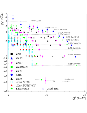
Figure 9: Left: Available world data on $g_{1}^{p}$ as of 2017. An offset $C(x_{Bj})$ is added to $g_{1}^{p}$ for visual clarity. Only two of the four energies of experiment EG1b are shown. The dotted lines mark a particular $x_{Bj}$ bin and do not represent the $Q^{2}$-evolution. Right: Same as left but for DIS data only. Despite the modest energy, part of JLab’s data reaches the DIS and, thanks to JLab’s high luminosity, they contribute significantly to the global data.

Global DIS data analyses [299]-[320] are discussed next. Their primary goal is to provide the polarized PDFs $\Delta q(x_{Bj})$ and $\Delta g(x_{Bj})$, as well as their integrals $\Delta\Sigma$ and $\Delta G$, which enter the spin sum rule, Eq. (31). Then, we present the specialized DIS experiments focusing on large $x_{Bj}$. Next, we review the information on the nucleon spin structure emerging from experiments with kinematics below the DIS. Afterward, we review the parton correlations (higher-twists) information obtained with these low energy data together with the DIS ones and the closely related phenomenon of hadron-parton duality. Finally, we conclude this section with our present knowledge on the nucleon spin at high energy, in particular the components of the spin sum rule, Eq. (31), and discuss the origin of their values. We conclude on the consistency of the data and remaining questions.

6.2 Global analyses

DIS experiments are analyzed in the pQCD framework. Their initial goal was to test QCD using the Bjorken sum rule, Eq. (55). After 25 years of studies, it is now checked to almost 5% level [321, 322, 323, 324]. Meanwhile, the nucleon spin structure started to be uncovered. Among the main results of these efforts is the determination of the small contribution of the quark spins $\Delta\Sigma$, Eq. (52), which implies that the quark OAM or/and of the gluon contribution $\Delta G+\mbox{L}_{g}$ are important. Global analyses, which now include not only DIS but SIDIS, p-p and $e^{+}$-$e^{-}$ collisions provide fits of PDFs and are the main avenue of interpreting the data [299, 306, 315, 313, 317]. These analysis are typically at NLO in $\alpha_{s}$, although NNLO has become available recently [103]. Several groups have carried out such analyses. Beside data, the analyses are constrained by general principles, including positivity constraints (see Section 3.1.8) and often other constraints such as SU(2)_f and SU(3)_f symmetries (see Section 5.5), counting rules [31] and integrability (i.e., the matrix elements of the axial current are always finite). A crucial difference between the various analyses is the choice of initial PDF ansatz, particularly for $\Delta g(x_{Bj})$, and of methods to minimize the bias stemming from such choice, which is the leading contribution to the systematic uncertainty. Two methods are used to optimize the PDFs starting from the original ansatz. One is to start from polynomial PDFs and optimize them with respect to the data and general constraints using Lagrange multipliers or Hessian techniques. The other approach determines the best PDFs using neural networks. Other differences between analyses are the choice of renormalization schemes (recent analyses typically use $\overline{MS}$), of factorization schemes and of factorization scale. Observables are in principle independent of these arbitrary choices but not in practice because of the necessary truncation of the pQCD series: calculating perturbative coefficients at high orders quickly becomes overbearing. Furthermore, pQCD series are Poincaré series that diverge beyond an order approximately given by $\pi/\alpha_{s}$. Thus, they must be truncated at or before this order. However, at the typical scale $\mu^{2}=5$ GeV², $\pi/\alpha_{s}\approx 11$ so this is currently not a limitation. The truncations make the perturbative approximant of an observable to retain a dependence on the arbitrary choices made by the DIS analysts. In principle, this dependence decreases with $Q^{2}$: at high enough $Q^{2}$ where the observable is close to the LO value of its perturbative approximant, unphysical dependencies should disappear since LO is renormalization scheme independent (with some exceptions however, such as non-zero renormalons [91]. Another noticeable example is $\Delta\Sigma$’s perturbative approximant which contains a non-vanishing contribution at $Q^{2}\to\infty$ from the gluon anomaly, see Section 5.5). Evidently, at finite $Q^{2}$, observables also depend on the $\alpha_{s}$ order at which the analysis is carried out. DIS analysis accuracy is limited by these unphysical dependencies. Optimization methods exist to minimize them. For instance, the factorization scale $\mu$ can be determined by comparing nonperturbative calculations to their corresponding perturbative approximant, see e.g., Refs. [156, 157]. That $\mu$ depends on the renormalization scheme (and of the pQCD order) illustrates the discussion: at N³LO $\mu=0.87\pm 0.04$ GeV in the $\overline{MS}$ scheme, $\mu=1.15\pm 0.06$ GeV in the $MOM$ scheme and $\mu=1.00\pm 0.05$ GeV in the $V$ scheme. Another example of optimization procedure is implementing the renormalization group criterium that an observable cannot depend on conventions such as the renormalization scheme choice. Optimizing a pQCD series is then achieved by minimizing the renormalization scheme dependence. One such approach is the BLM procedure [94]. The Principle of Maximum Conformality (PMC) [95] generalizes it and sets unambiguously order-by-order in pQCD the renormalization scale, i.e., the scale at which the renormalization procedure subtracts the ultraviolet divergences (often also denoted $\mu$ but not to be confused with the factorization scale just discussed). By fulfilling renormalization group invariance the PMC provides approximants independent of the choice of renormalization scheme.

While polarized DIS directly probes $\Delta q(x_{Bj},Q^{2})$, $\Delta g(x_{Bj},Q^{2})$ is also accessed through the pQCD evolution equations, Eq. (27). However, the present precision and kinematics coverage of the data do not constrain it well. It will be significantly improved by the 12 GeV spin program at JLab that will cover the largely unconstrained $x_{Bj}>0.6$ region, and by the polarized EIC (electron-ion collider) that will cover the low-$x_{Bj}$ domain [327]. (The EIC may also constrain the gluon OAM [328]). But $\Delta g(x_{Bj},Q^{2})$ is best accessed via semi-exclusive DIS involving photon-gluon fusion, $\gamma^{*}g\to q\overline{q}$. This was evaluated by the SMC, HERMES and COMPASS experiments. Polarized p-p (RHIC-spin) provides other channels that efficiently access $\Delta g(x_{Bj},Q^{2})$, see Section 2.2.

Global analysis results are discussed in Section 6.11 which gives the current picture of the nucleon spin structure at high energy. They are listed in Tables 3-8 in the Appendix.

6.3 PQCD in the high-$x_{Bj}$ domain

The high-$x_{Bj}$ region should be relatively simple: as $x_{Bj}$ grows, the valence quark distribution starts prevailing over the ones of gluons and of $q$-$\overline{q}$ pairs materializing from gluons, see Fig. 7. This prevalence allows the use of constituent quark models (see page 3.2.1) [109]. Thus the high-$x_{Bj}$ region is particularly interesting. It has been studied with precision by the JLab collaborations E99-117, EG1b, E06-014 and EG1dvcs, and by the CERN’s COMPASS collaboration.

This region has been precisely studied only recently since there, unpolarized PDFs (Fig. 7) are small, which entails small cross-sections that, furthermore, have kinematic factors varying at first order as $1/x_{Bj}$. Thus, early data high-$x_{Bj}$ lacked the precision necessary to extract polarized PDF. The high polarized luminosity of JLab has allowed to explore this region more precisely.

6.3.1 $A_{1}$ in the DIS at high-$x_{Bj}$

Assuming that quarks are in a $S$ state, i.e., they have no OAM, a quark carrying all the nucleon momentum ($x_{Bj}\to 1$) must carry the nucleon helicity [329]. This implies $A_{1}\xrightarrow[x_{Bj}\to 1]{}1$. This is a rare example of absolute prediction from QCD: generally pQCD predicts only the $Q^{2}$-dependance of observables, see Sections 3.1.1 and 3.1.9. (Other examples are the processes involving the chiral anomaly, such as $\pi^{0}\to\gamma\gamma$.) Furthermore, the valence quarks dominance makes known the nucleon wavefunction, see Eq. (36). The BBS [33] and LSS [304]) global fits include these two constraints. The $x_{Bj}$-range where the $S$-state dominates is the only significant assumption of these fits which have been improved to include the $\left|\mbox{L}_{z}(x_{Bj})\right|=1$ wavefunction components [150]. The phenomenological predictions [33, 150, 304] for $A_{1}(x_{Bj}\to 1)$ are thus based on solid premises. Model predictions also exist and are discussed next.

6.3.2 Quark models and other predictions of $A_{1}$ for high-$x_{Bj}$ DIS

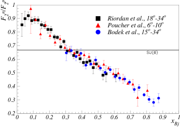
Figure 10: $F_{2}^{n}/F_{2}^{p}$ SLAC data [330]. SU(6) predicts $F_{2}^{n}/F_{2}^{p}=2/3$.

Modeling the nucleon as made of three constituent quarks is justified in the high-$x_{Bj}$ DIS domain since there, valence quarks dominate. This finite number of partons and the SU(6) flavor-spin symmetry allow one to construct a simple nucleon wavefunction, see Eq. (36), leading to $A_{1}^{p}=5/9$ and $A_{1}^{n}=0$. However SU(6) is broken, as clearly indicated e.g., by the nucleon-$\Delta$ mass difference of 0.3 GeV or the failure of the SU(6) prediction that $F_{2}^{n}/F_{2}^{p}=2/3$, see Fig. 10. The one-gluon exchange (pQCD “hyperfine interaction”, see page 3.2.1) breaks SU(6) and can account for the nucleon-$\Delta$ mass difference. It predicts the same $x_{Bj}\to 1$ limits as for pQCD: $A_{1}^{p}=A_{1}^{n}=1$. A prediction of the constituent quark model improved with the hyperfine interaction [331] is shown in Fig. 11.

Another approach to refine the constituent quark model is using chiral constituent quark models [332]. Such models assume a $\approx 1$ GeV scale for chiral symmetry breaking, significantly higher than $\Lambda_{s}$ ($0.33$ GeV in the $\overline{MS}$ scheme) and use an effective Lagrangian [333] with valence quarks interacting via Goldstone bosons as effective degrees of freedom. The models include sea quarks. $x_{Bj}$-dependence is included phenomenologically in recent models, e.g., in the prediction [334].

Augmenting quark models with meson clouds provides another possible SU(6) breaking mechanism [115, 149]. Ref. [335] compares $A_{1}$ predictions with this approach and that of the “hyperfine” mechanism.

Other predictions for $A_{1}$ at high-$x_{Bj}$ exist and are shown in Fig. 11. They are:

$\bullet$ The statistical model of Ref. [336]. It describes the nucleon as fermionic and bosonic gases in equilibrium at an empirically determined temperature;

$\bullet$ The hadron-parton duality (Section 6.10). It relates well-measured baryons form factors (elastic or $\Delta(1232)~{}3/2^{+}$ reactions, all at high-$x_{Bj}$) to DIS structure functions at the same $x_{Bj}$ [337]. Predictions depend on the mechanism chosen to break SU(6), with two examples shown in Fig. 11;

$\bullet$ Dyson-Schwinger Equations with contact or realistic interaction. They predict $A_{1}(1)$ values significantly smaller than pQCD [174];

$\bullet$ The bag model of Boros and Thomas, in which three free quarks are confined in a sphere of nucleon diameter. Confinement is provided by the boundary conditions requiring that the quark vector current cancels on the sphere surface [338].

$\bullet$ The quark model of Kochelev [339] in which the quark polarization is affected by instantons representing non-perturbative fluctuations of gluons.

$\bullet$ The chiral soliton models of Wakamatsu [340] and Weigel et al. [341] in which the quark degrees of freedom explicitly generate the hadronic chiral soliton properties of the Skyrme nucleon model.

$\bullet$ The quark-diquark model of Cloet et al. [342].

6.3.3 $A_{1}$ results

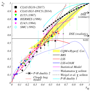
Figure 11: $A_{1}$ DIS data on the proton (left) and neutron (right). The $Q^{2}$ values of the various results are not necessarily the same, but $A_{1}$’s $Q^{2}$-dependence is weak.

Experimental results on $A_{1}$ [257, 267, 279, 280, 282, 283, 288, 291] are shown in Fig. 11. They confirm that SU(6), whose prediction is shown by the flat lines in Fig. 11, is broken. The $x_{Bj}$-dependence of $A_{1}$ is well reproduced by the constituent quark model with “hyperfine” corrections. The systematic shift for $A_{1}^{n}$ at $x_{Bj}<0.4$ may be a sea quark effect. The BBS/LSS fits to pre-JLab data disagrees with these data. The fits are constrained by pQCD but assume no quark OAM. Fits including it [150] agree with the data, which suggests the importance of the quark OAM. However, the relation between the effect of states $\left|\mbox{L}_{z}(x_{Bj})\right|=1$ at high $x_{Bj}$ and $\Delta L$ in Eq. (31) remains to be elucidated. To solve this issue, the nucleon wavefunction at low $x_{Bj}$ must be known. While the data have excluded some of the models (bag model [338], or specific SU(6) breaking mechanisms in the duality approach), high-precision data at higher $x_{Bj}$ are needed to test the remaining predictions. Such data will be taken at JLab in 2019 [343].

6.4 Results on the polarized partial cross-sections $\sigma_{TT}$ and $\sigma_{LT}^{\prime}$

The pairs of observables ($g_{1}$, $g_{2}$), ($A_{1}$, $A_{2}$), or ($\sigma_{TT}$, $\sigma_{LT}^{\prime}$) all contain identical spin information. $A_{1}$ at high-$x_{Bj}$ was discussed in the previous section. The $g_{1}$ DIS data at smaller $x_{Bj}$ are discussed in the Section 6.11, and the $g_{2}$ data are discussed in Section 6.9.3. Here, $\sigma_{TT}$ and $\sigma_{LT}^{\prime}$, Eq. (17), are discussed.

Data on $\sigma_{TT}$ and ${\sigma}_{LT}^{\prime}$ on ³He are available in the strong-coupling QCD region [275, 287] for $0.04<Q^{2}<0.90$ GeV² and $0.9<W<2$ GeV. Neutron data are unavailable since for $x_{Bj}$-dependent quantities such as $g_{1}$ or $\sigma_{TT}$, there is no known accurate method to extract the neutron from ³He. Yet, since in ³He, protons contribute little to polarized observables, the results of Refs. [275, 287] suggest how neutron data may look like. Neutron information can be extracted for moments, see Sections 6.5 and 5.2.

A large trough is displayed at the $\Delta(1232)~{}3/2^{+}$ resonance by $\sigma_{TT}$. It is also present for other resonances, but not as marked. The $\Delta(1232)~{}3/2^{+}$ dominates because it is the lightest resonance (see Eq. (17)) and because its spin 3/2 makes the nucleon-$\Delta$ transition largely transverse. Since $\sigma_{TT}=(\sigma_{T,1/2}-\sigma_{T,3/2})/2$, where 1/2 and 3/2 refer to the spin of the intermediate state, here the $\Delta(1232)~{}3/2^{+}$, $\sigma_{TT}$ is maximum and negative. At large $Q^{2}$, chiral symmetry is restored, which forbids spin-flips and makes $\sigma_{T,1/2}$ dominant. This shrinkage of the $\Delta(1232)~{}3/2^{+}$ trough is seen in the $1\leq Q^{2}\leq 3.5$ GeV² data used to study duality, Section 6.10. All this implies that at low $Q^{2}$ the $\Delta(1232)~{}3/2^{+}$ contribution dominates the generalized GDH integral ($\propto\int\sigma_{TT}/\nu\,d\nu$), a dominance further amplified by the $1/\nu$ factor in the integral. This latest effect is magnified in higher moments, such as those of generalized polarizabilities, Eqs. (46) and (48).

${\sigma}_{LT}^{\prime}$ is rather featureless compared to $\sigma_{TT}$ and in particular shows no structure at the $\Delta(1232)~{}3/2^{+}$ location. It confirms that the nucleon-to-$\Delta$ transition occurs mostly via spin-flip (magnetic dipole transition) induced by transversely polarized photons. The longitudinal photons contributing little, the longitudinal-transverse interference cross-section ${\sigma}_{LT}^{\prime}$ is almost zero. At higher $W$, ${\sigma}_{LT}^{\prime}$ becomes distinctly positive.

6.5 Results on the generalized GDH integral

The generalized GDH integral $I_{TT}(Q^{2})$, Eq. (44), was measured for the neutron and proton at DESY (HERMES) [344] and JLab [243, 275, 287]. The measurements cover the energy range from the pion production threshold up to typically $W\approx 2.0$ GeV. The higher-$W$ contribution is estimated with parameterizations, e.g., that of Ref. [345]. At low $Q^{2}$, $I_{TT}$ can be computed using $\chi$PT [208, 209, 210, 211, 212, 213, 214]. The Ji-Kao-Lensky et al. calculations [210, 212, 214] and data agree, up to about $Q^{2}=0.2$ GeV². After this, the calculation uncertainties become too large for a relevant comparison. The Bernard et al. calculations and data [209, 208, 213] also agree, although marginally. The MAID model underestimates the data [247]. ($I_{TT}(Q^{2})$ constructed with MAID is integrated only up to $W\leq 2$ GeV and thus must be compared to data without large-$W$ extrapolation. The extrapolation of the p+n data [243] together with the proton GDH sum rule world data [242] yield $I_{TT}^{n}(0)=-0.955\pm 0.040\,(stat)\pm 0.113\,(syst)$, which agrees with the sum rule expectation.

6.6 Moments of $g_{1}$ and $g_{2}$

6.6.1 Extractions of the $g_{1}$ first moments

$\Gamma_{1}^{p}$ and $\Gamma_{1}^{n}$ moments: The measured $\Gamma_{1}(Q^{2})$ is constructed by integrating $g_{1}$ from $x_{Bj,min}$ up to the pion production threshold. $x_{Bj,min}$, the minimum $x_{Bj}$ reached, depends on the beam energy and minimum detected scattering angle for a given $Q^{2}$ point. Table 1 on page 1 provides these limits. When needed, contributions below $x_{Bj,~{}min}$ are estimated using low-$x_{Bj}$ models [345, 346]. For the lowest $Q^{2}$, typically below the GeV² scale, the large-$x_{Bj}$ contribution (excluding elastic) is also added when it is not measured. The data for $\Gamma_{1}$, shown in Fig. 12, are from SLAC [267]-[270], CERN [114, 271]-[347, 348, 324, 321]-[323], DESY [344] and JLab [275]-[280, 282, 285, 286]-[288, 349, 350].

Bjorken sum $\Gamma_{1}^{p-n}$: The proton and neutron (or deuteron) data can be combined to form the isovector moment $\Gamma_{1}^{p-n}$. The Bjorken sum rule predicts that $\Gamma_{1}^{p-n}\xrightarrow[Q^{2}\to\infty]{}g_{A}/6$ [235]. The prediction is generalized to finite $Q^{2}$ using OPE, resulting in a relatively simple leading–twist $Q^{2}$-evolution in which only non-singlet coefficients remain, see Eq. (54). The sum rule has been experimentally validated, most precisely by E155 [257]: $\Gamma_{1}^{p-n}=0.176\pm 0.003\pm 0.007$ at $Q^{2}$ = 5 GeV², while the sum rule prediction at the same $Q^{2}$ is $\Gamma_{1}^{p-n}=0.183\pm 0.002$. $\Gamma_{1}^{p-n}$ was first measured by SMC [271] and then E143 [268], E154 [256], E155 [257] and HERMES [344]. Its $Q^{2}$-evolution was mapped at JLab [282, 349, 350]. The latest measurement (COMPASS) yields $\Gamma_{1}^{p-n}=0.192\pm 0.007$ (stat) $\pm 0.015$ (syst) [321, 322, 323, 324, 348].
As an isovector quantity, $\Gamma_{1}^{p-n}$ has no $\Delta(1232)~{}3/2^{+}$ resonance contribution. This simplifies $\chi$PT calculations, which may remain valid to higher $Q^{2}$ than typical for $\chi$PT [351]. In addition, a non-singlet moment is simpler to calculate with LGT since the CPU-expensive disconnected diagrams (quark loops) do not contribute. (Yet, the axial charge $g_{A}$ and the axial form factor $g_{A}(Q^{2})$ remain a challenge for LGT [352] because of their strong dependence to the lattice volume. Although the calculations are improving [353], the LGT situation for $g_{A}$ is still unsatisfactory.) Thus, $\Gamma_{1}^{p-n}$ is especially convenient to test the techniques discussed in Section 4. As for all moments, a limitation is the impossibility to measure the $x_{Bj}\to 0$ contribution, which would require infinite beam energy. The Regge behavior $g_{1}^{p-n}(x_{Bj})=(x_{0}/x_{Bj})^{0.22}$ may provide an adequate low-$x_{Bj}$ extrapolation [346] (see also [99, 100, 101]).

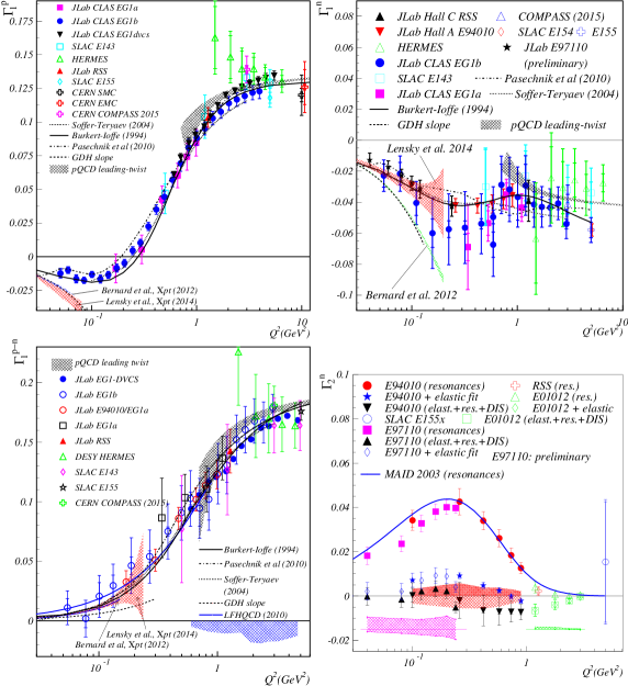
Figure 12: The moments $\Gamma_{1}^{p}$ (top left), $\Gamma_{1}^{n}$ (top right) and the Bjorken integral (bottom left), all without elastic contribution. The derivatives at $Q^{2}=0$ are predicted by the GDH sum rule. In the DIS, the leading-twist pQCD evolution is shown by the gray band. Continuous lines and bands at low $Q^{2}$ are $\chi$PT predictions. $\Gamma_{2}^{n}$, with and without elastic contribution, is shown on the lower right panel wherein the upper bands are experimental systematic uncertainties. The lower bands in the figure are the systematic uncertainties from the unmeasured part below $x_{Bj,min}$. ($\Gamma_{2}^{p}$ is not shown since only two points, from E155x and RSS, are presently available.) The Soffer-Teryaev [354], Burkert-Ioffe [355], Pasechnik et al. [356] and MAID [247] models are phenomenological parameterizations.

6.6.2 Data and theory comparisons

At $Q^{2}=0$, the GDH sum rule, Eq. (45), predicts $d\Gamma_{1}/dQ^{2}$ (see Fig. 12). At small $Q^{2}$, $\Gamma_{1}(Q^{2})$ can be computed using $\chi$PT. The comparison between data and $\chi$PT results on moments is given in Table 2 in which one sees that in most instances, tensions exist between data and claculations of $\Gamma_{1}$.

Table 2: Comparison between $\chi$PT results and data for moments. The bold symbols denote moments for which $\chi$PT was expected to provide robust predictions. “A” means that data and calculations agree up to at least $Q^{2}=0.1$ GeV², “X” that they disagree and “-” that no calculation is available. The $p+n$ superscript indicates either deuteron data without deuteron break-up channel, or proton+neutron moments added together with neutron information either from D or ³He.

Ref.	$\Gamma_{1}^{p}$	$\Gamma_{1}^{n}$	$\boldsymbol{\Gamma_{1}^{p-n}}$	$\Gamma_{1}^{p+n}$	$\gamma_{0}^{p}$	$\gamma_{0}^{n}$	$\boldsymbol{\gamma_{0}^{p-n}}$	$\gamma_{0}^{p+n}$	$\boldsymbol{\delta_{LT}^{n}}$	$d_{2}^{n}$
Ji 1999 [210, 211]	X	X	A	X	-	-	-	-	-	-
Bernard 2002 [208, 209]	X	X	A	X	X	A	X	X	X	X
Kao 2002 [212]	-	-	-	-	X	A	X	X	X	X
Bernard 2012 [213]	X	X	A	X	X	A	X	X	X	-
Lensky 2014 [214]	X	A	A	A	A	X	X	X	$\sim$ A	A

The models of Soffer-Teryaev [354], Burkert-Ioffe [355] and Pasechnik et al. [356] agree well with the data, as does the LFHQCD calculation [357]. The Soffer-Teryaev model uses the weak $Q^{2}$-dependence of $\Gamma_{T}=\Gamma_{1}+\Gamma_{2}$ to robustly interpolate $\Gamma_{T}$ between its zero value and known derivative at $Q^{2}=0$ and its known values at large $Q^{2}$. $\Gamma_{1}$ is obtained from $\Gamma_{T}$ using the BC sum rule, Eq. (50), where PQCD radiative corrections and higher-twists are accounted for. Pasechnik  et al. improved this model by using for the pQCD and higher-twist corrections a strong coupling $\alpha_{s}$ analytically continued at low-$Q^{2}$, which removes the unphysical Landau-pole divergence at $Q^{2}=\Lambda_{s}^{2}$, and minimizes higher-twist effects [91]. This extends pQCD calculations to lower $Q^{2}$ than typical. The improved $\Gamma_{1}$ is continued to $Q^{2}=0$ by using $\Gamma_{1}(0)=0$ and $d\Gamma_{1}(0)/dQ^{2}$ from the GDH sum rule. The Burkert-Ioffe model is based on a parameterization of the resonant and non-resonant amplitudes [358], complemented with a DIS parameterization [236] based on vector dominance. In LFHQCD, the effective charge $\alpha_{g_{1}}$ (viz the coupling $\alpha_{s}$ that includes the pQCD gluon radiations and higher-twist effects of $\Gamma_{1}^{p-n}$ [91]) is computed and used in the leading order expression of the Bjorken sum to obtain $\Gamma_{1}^{p-n}$.

The leading-twist $Q^{2}$-evolution is shown in Fig. 12 (gray bands). The values $a_{8}$ = 0.579, $g_{A}$ = 1.267 and $\Delta\Sigma^{p}$ = 0.15 ($\Delta\Sigma^{n}$ = 0.35) are used to anchor the $\Gamma_{1}^{p(n)}$ evolutions, see Eq. (52). For $\Gamma_{1}^{p-n}$, $g_{A}$ suffices to fix the absolute scale. In all cases, leading-twist pQCD follows the data down to surprisingly low $Q^{2}$, exhibiting hadron-parton global duality i.e., an overall suppression of higher-twists, see Sections 6.9 and 6.10.

6.6.3 Results on $\Gamma_{2}$ and on the BC and ELT sum rules

Neutron results: $\Gamma_{2}^{n}(Q^{2})$ from E155x [270], E94-010 [275], E01-012 [285], RSS [278] and E97-110 [287] is shown in Fig. 12. Except for E155x for which the resonance contribution is negligible, measurements comprise essentially the whole resonance region. This region contributes positively and significantly yielding $\Gamma_{2}^{n,res.}\approx-\Gamma_{1}^{n,res.}$, as expected since there, $g_{2}\approx-g_{1}$ (see Section 6.9.3). The MAID parameterization (continuous line) agrees well with these data. The elastic contribution, estimated from the parameterization in Ref. [359], is of opposite sign and nearly cancels the resonance contribution, as expected from the BC sum rule $\Gamma_{2}(Q^{2})=0$. The unmeasured part below $x_{Bj,min}$ is estimated assuming $g_{2}=g_{2}^{WW}$, see Eq. (60). (While at leading-twist $g_{2}^{WW}$ satisfies the BC sum rule, $\int g_{2}^{WW}dx=0$, the low-$x_{Bj}$ contribution is the non-zero partial integral $\int_{0}^{x_{Bj,min}}g_{2}(Q^{2},y)dy=x_{Bj,min}\big{[}g_{2}^{WW}(Q^{2},x_{Bj,min})+g_{1}(Q^{2},x_{Bj,min})\big{]}$.) The resulting $\Gamma_{2}^{n}$ fulfills the BC sum rule. The interesting fact that the elastic contribution nearly cancels that of the resonances accounts for the sum rule validity at low and moderate $Q^{2}$.

Proton results: The E155x proton result ($Q^{2}=5$ GeV²) [270] agrees with the BC sum rule: $\Gamma_{2}^{p}=-0.022\pm 0.022$ where, as for the JLab data, a 100% uncertainty is assumed on the unmeasured low-$x_{Bj}$ contribution estimated to be 0.020 using Eq. (60). Neglecting higher-twists for the low-$x_{Bj}$ extrapolation, RSS yields, $\Gamma_{2}^{p}=\big{(}-6\pm 8$(stat)$\pm 20$(syst))$\times 10^{-4}$ at $Q^{2}=1.28$ GeV² [278], which agrees with the BC sum rule. Finally $g_{2}^{p}$ has been measured at very low $Q^{2}$ [326], from which $\Gamma_{2}^{p}$ should be available soon.

Conclusion: Two conditions for the BC sum rule validity are that 1) $g_{2}$ is well-behaved, so that $\Gamma_{2}$ is finite, and 2) $g_{2}$ is not singular at $x_{Bj}=0$. The sum rule validation implies that the conditions are satisfied. Moreover, since $g_{2}^{WW}$ fulfills the sum rule at large $Q^{2}$, these conclusions can be applied to twist 3 contribution describing the quark-gluon correlations. Finally, since the sum rule seems verified from $Q^{2}\sim 0$ to 5 GeV² and since the contributions of twist-$\tau$ are $Q^{2-\tau}$-suppressed, the conclusion ensuring that the $g_{2}$ function is regular should be true for all the terms of the twist series that represents $g_{2}$.

The Efremov-Leader-Teryaev sum rule: The ELT sum rule, Eq. (65), is compatible with the current world data. However, the recent global PDF fit KTA17 [320] indicates that the sum rule for $n=2$ and twist 2 contribution only is violated at $Q^{2}=5$ GeV², finding $\int_{0}^{1}x\big{(}g_{1}+2g_{2}\big{)}dx=0.0063(3)$ rather than the expected null sum. If this is true, it would suggest a contribution of higher-twists even at $Q^{2}=5$ GeV².

6.7 Generalized spin polarizabilities $\gamma_{0}$, $\delta_{LT}$

Generalized spin polarizabilities offer another test of strong QCD calculations. Contrary to $\Gamma_{1}$ or $\Gamma_{2}$, the kernels of the polarizability integrals, Eqs. (46) and (48), have a $1/\nu^{2}$ factor that suppresses the low-$x_{Bj}$ contribution. Hence, polarizability integrals converge faster and have smaller low-$x_{Bj}$ uncertainties. At low $Q^{2}$, generalized polarizabilities have been calculated using $\chi$PT, see Table 2. It is difficult to include in these calculations the resonances, in particular $\Delta(1232)~{}3/2^{+}$. It was however noticed that this excitation is suppressed in $\delta_{LT}$, making it ideal to test $\chi$PT calculations for which the $\Delta(1232)~{}3/2^{+}$ is not included, or included phenomenologically [212, 208]. Measurements of $\gamma_{0}$ and $\delta_{LT}$ are available for the neutron (E94-010 and E97-110) for $0.04<Q^{2}<0.9$ GeV² [275, 287]. JLab CLAS results are also available for $\gamma_{0}$ for the proton, neutron and deuteron [280, 279, 282, 243] for approximately $0.02<Q^{2}<3$ GeV².

6.7.1 Results on $\gamma_{0}$

The $\gamma_{0}^{n}$ extracted either from ³He [275] or D [279] agree well with each other. The MAID phenomenological model [247] agrees with the $\gamma_{0}^{n}$ data, and so do the $\chi$PT results (Table 2), except the recent Lensky et al. calculation [214]. For $\gamma_{0}^{p}$, the situation is reversed: only Ref. [214] agrees well with the data, but not the others (including MAID). This problem motivated an isospin analysis of $\gamma_{0}$ [350] since, e.g. axial-vector meson exchanges in the $t-$channel (short-range interaction) that are not included in computations could be important for only one of the isospin components of $\gamma_{0}$. $\chi$PT calculations disagree with $\gamma_{0}^{p+n}$ but MAID agrees. Alhough the $\Delta(1232)~{}3/2^{+}$ is suppressed in $\gamma_{0}^{p-n}$, $\chi$PT disagrees with the data. Thus, the disagreement on $\gamma_{0}^{p}$ and $\gamma_{0}^{n}$ cannot be assigned to the $\Delta(1232)~{}3/2^{+}$. MAID also disagrees with $\gamma_{0}^{p-n}$.

6.7.2 The $\delta_{LT}$ puzzle

Since the $\Delta(1232)~{}3/2^{+}$ is suppressed in $\delta_{LT}$, it was expected that its $\chi$PT calculation would be robust. However, the $\delta_{LT}^{n}$ data [275] disagreed with the then available $\chi$PT results. This discrepancy is known as the “$\delta_{LT}$ puzzle”. Like $\gamma_{0}$, an isospin analysis of $\delta_{LT}$ may help with this puzzle. The needed $\delta_{LT}^{p}$ data are becoming available [326]. The second generation of $\chi$PT calculations on $\delta_{LT}^{n}$ [213, 214] agrees better with the data. At larger $Q^{2}$ (5 GeV²), the E155x data [270] agree with a quenched LGT calculation [190, 191]. At large $Q^{2}$, generalized spin polarisabilities are expected to scale as $1/Q^{6}$, with the usual additional softer dependence from pQCD radiative corrections [205, 234]. Furthermore, the Wandzura-Wilczek relation, Eq. (60), relates $\delta_{LT}$ to $\gamma_{0}$:

$$\vspace{-0.3cm}\delta_{LT}(Q^{2})\to{\frac{1}{3}}\gamma_{0}(Q^{2})\ \ \ {\rm if~{}}g_{2}\approx g_{2}^{WW}$$ (67)

The available data being mostly at $Q^{2}<1$ GeV², this relation and the scaling law have not been tested yet. Furthermore, the signs of the $\gamma_{0}$ and $\delta_{LT}$ data disagree with Eq. (67). These facts are not worrisome: for $\Gamma_{1}$ and $\Gamma_{2}$, scaling is observed for $Q^{2}\gtrsim 1$ GeV², when the overall effect of higher-twists decreases. For higher moments, resonances contribute more, so scaling should begin at larger $Q^{2}$. The violation of Eq. (67) is consistent with the fact that $g_{2}\neq g_{2}^{WW}$ in the resonance domain, see Section 6.9.3.

6.8 $d_{2}$ results

Another combination of second moments, $d_{2}$ (Eqs. (58) and (59)), is particularly interesting because it is interpreted as part of the transverse confining force acting on quarks [38, 39], see Section 6.9.2. Furthermore, $d_{2}$ offers another possibility to study the nucleon spin structure at large $Q^{2}$ since it has been calculated by LGT [190, 191, 360] and modeled with LC wave functions [45]. $d_{2}$ can also be used to study the transition between large and small $Q^{2}$. $\overline{d_{2}}(Q^{2})$ is shown in Fig. 13 (the bar over $d_{2}$ indicates that the elastic contribution is excluded). The experimental results are from JLAB (neutron from ³He [275, 283, 285, 290] and from D [278], and proton [277]), from SLAC (neutron from D and proton) [270], and from global analyses (JAM [313, 361], KTA17 [320]), which contain only DIS contributions.

6.8.1 Results on the neutron

At moderate $Q^{2}$, $\overline{d_{2}}^{n}$ is positive and reaches a maximum at $Q^{2}\gtrsim 0.4$ GeV². Its sign is uncertain at large $Q^{2}$. At low $Q^{2}$ the comparison with $\chi$PT is summarized in Table 2. MAID agrees with the data. That MAID and the RSS datum (both covering only the resonance region) match the DIS-only global fits and E155x datum suggests that hadron-parton duality is valid for $d_{2}^{n}$, albeit uncertainties are large. The LGT [190, 191, 360], Sum Rule approach [362], Center-of-Mass bag model [363] and Chiral Soliton model [364] all yield a small $d_{2}^{n}$ at $Q^{2}>1$ GeV², which agrees with data. At these large $Q^{2}$, the data precision is still insufficient to discriminate between these predictions. The negative $d_{2}^{n}$ predicted with a LC model [45] disagrees with the data.

6.8.2 Results on the Proton

Proton data are scarce, with a datum from RSS [277] and one from E155x [270]. In Fig. 13, the RSS point was evolved to the E155x $Q^{2}$ assuming the $1/Q$-dependence expected for a twist 3 dominated quantity (neglecting the weak log dependence from pQCD radiation). The E155x and RSS results agree although RSS measured only the resonance contribution. As for $d_{2}^{n}$, this suggests that hadron-parton duality is valid for $d_{2}^{p}$. However, this conclusion is at odds with the mismatch between the (DIS-only) JAM global PDF fit [361] and the (resonance-only) result from RSS.

6.8.3 Discussion

Overall, $\overline{d_{2}}$ is small compared to the twist 2 term ($|\Gamma_{1}|\approx 0.1$ typically at $Q^{2}=1$ GeV², see Fig. 12) or to the twist 4 term ($f_{2}\approx 0.1$, see Fig. 14). This smallness was predicted by several models. The high-precision JLab experiments measured a clearly non-zero $\overline{d_{2}}$. More data for $\overline{d_{2}^{p}}$ are needed and will be provided shortly at low $Q^{2}$ [326] and in the DIS [289], see Table 1. Then, the 12 GeV upgrade of JLAB will provide $\overline{d_{2}}$ in the DIS with refined precision, in particular with the SoLID detector [365].

Figure 13: $\overline{d_{2}}$ data from SLAC, JLab and PDF global analyses, compared to LGT [190, 191, 360], $\chi$PT [209, 214] and models [45, 362, 363, 364]. Left panel: neutron data (the inner error bars are statistical. The outer ones are for the systematic and statistic uncertainties added in quadrature). Right: proton data.

6.9 Higher-twist contributions to $\Gamma_{1}$, $g_{1}$ and $g_{2}$

Knowledge of higher-twists is important since for inclusive lepton scattering, they are the next nonperturbative distributions beyond the PDFs, correlating them. higher-twists thus underlie the parton-hadron transition, i.e., the process of strengthening the quark binding as the probed distance increases. In fact, some higher-twists are interpreted as confinement forces [38, 39]. Furthermore, knowing higher-twists permits one to set the limit of applicability to pQCD and extend it to lower $Q^{2}$, see e.g., Massive Perturbation Theory [356, 366]. Despite their phenomenological importance, higher-twists have been hard to measure accurately because they are often surprisingly small.

6.9.1 Leading and higher-twist analysis of $\Gamma_{1}$

Figure 14: Top: twist coefficients $\mu_{i}$ vs. $i$. The lines linking the points show the oscillatory behavior. Bottom: twist 4 $f_{2}$. Newer results (e.g., EG1dvcs) include the older data (e.g., EG1a).

The higher-twist contribution to $\Gamma_{1}$ can be obtained by fitting its data with a function conforming to Eqs. (51)-(52) and (54)-(55). The perturbative series is truncated to an order relevant to the data accuracy. Once $\mu_{4}$ is extracted, the pure twist 4 matrix element $f_{2}$ is obtained by subtracting $a_{2}$ (twist 2) and $d_{2}$ (twist 3) from Eq. (55). For $\Gamma_{1}^{p,n}$, $\mu_{2}^{p,n}$ is set by fitting high-$Q^{2}$ data, e.g., $Q^{2}\geq 5$ GeV², and assuming that higher-twists are negligible there. For $\Gamma_{1}^{p-n}$, $\mu_{2}^{p-n}$ is set by $g_{A}=1.2723(23)$ [18]. The resulting $\mu_{2}^{p,n}$, together with $a_{8}$ from the hyperons $\beta$-decay, yield $\Delta\Sigma=0.169\pm 0.084$ for the proton and $\Delta\Sigma=0.35\pm 0.08$ for the neutron [282, 367, 368]. The discrepancy may come from the low-$x_{Bj}$ part of $\Gamma_{1}^{n}$, which is still poorly constrained, as the COMPASS deuteron data [272] suggest. Specifically, it may be the low-$x_{Bj}$ contribution to the isoscalar quantity $\Gamma_{1}^{n+p}$, since $\Gamma_{1}^{p-n}$ agrees well with the Bjorken sum rule. Another possibility is a SU(3)_f violation. The $\Delta\Sigma$ obtained from global analyses (see Section 6.11) mix the proton and neutron data and agree with the averaged value of $\Delta\Sigma^{p}$ and $\Delta\Sigma^{n}$.

Fit results [282, 290, 349, 350, 367, 368] are shown and compared to available calculations [262, 362, 369, 370, 371] in Fig. 14. There are no predictions yet for twists higher than $f_{2}$. We note the sign alternation between $\mu_{2}$, $\mu_{4}$ and $\mu_{6}$. All higher power corrections are folded in $\mu_{8}$, which is thus not a clean term and does not follow the alternation. This one decreases the higher-twist effects and could explain the global quark-hadron spin duality (see Section 6.10). The sign alternation is opposite for proton and neutron, as expected from isospin symmetry, see Eq. (52) in which the non-singlet $g_{A}/12\approx 0.1$ dominates the singlet terms $\Delta\Sigma/9\approx 0.03$ and $a_{8}/36\approx 0.008$. The discrepancy between $\Delta\Sigma^{p}$ and $\Delta\Sigma^{n}$ explains why the value of $f_{2}$ extracted from $\Gamma_{1}^{p-n}$ differs from the $f_{2}$ values extracted individually. Indeed, $\Delta\Sigma$ vanishes in the Bjorken sum rule whose derivation does not assume SU(3)_f symmetry.

Although the overall effect of higher-twists is small at $Q^{2}>1$ GeV², $f_{2}$ itself is large: $|f_{2}^{p}|\approx 0.1$, to compare to $\mu_{2}^{p}=0.105(5)$; $f_{2}^{n}\approx 0.05$ for $|\mu_{2}^{n}|=0.023(5)$; $|f_{2}^{p-n}|\approx 0.1$ for $\mu_{2}^{p-n}=0.141(11)$. These large values conform to the intuition that nonperturbative effects should be important at moderate $Q^{2}$. The smallness of the total higher-twist effect is due to the factor $M^{2}/9\approx 0.1$ in Eq. (55), and to the $\mu_{i}$ alternating signs. Such oscillation can be understood with vector meson dominance [372].

6.9.2 Color polarizabilities and confinement force

Electric and magnetic color polarizabilities can be determined using Eq. (66). For the proton, $\chi_{E}^{p}=-0.045(44)$ and $\chi_{B}^{p}=0.031(22)$ [282]. For the neutron, $\chi_{E}^{n}=0.030(17)$, $\chi_{B}^{n}=-0.023(9)$. The Bjorken sum data yield $\chi_{E}^{p-n}=0.072(78)$, $\chi_{B}^{p-n}=-0.020(49)$. These values are small and the proton and neutron have opposite signs. Since $f_{2}\gg d_{2}$, this reflects the dominance of the non-singlet term $g_{A}$. The electric and magnetic Lorentz transverse confinement forces are proportional to the color polarizabilities [38, 39]:

$$\vspace{-0.3cm}F^{y}_{E}=-\frac{M^{2}}{4}\chi_{E},~{}~{}~{}F_{B}=-\frac{M^{2}}{2}\chi_{B}.$$ (68)

Their size of a few $10^{-2}$ GeV² can be compared to the string tension $\sigma_{str}=0.18$ GeV² obtained from heavy quarkonia. Several coherent processes prominent for the proton and neutron, e.g., the $\Delta(1232)~{}3/2^{+}$, are nearly inexistent for $\Gamma_{1}^{p-n}$ [351]. This may explain why $\Gamma_{1}^{p-n}$ is suited to extract $\alpha_{s}$ at low $Q^{2}$ [91, 373].

6.9.3 Higher-twist studies for $g_{1}$, $A_{1}$, $g_{2}$ and $A_{2}$

Figure 15: Top: $g_{1}^{n}(Q^{2})$ from E97103 (symbols). The inner error bars give the statistical uncertainty while outer bars are the systematic and statistical uncertainties added in quadrature. The continuous line is a global fit of the world data on $g_{1}^{n}$ [375], with its uncertainty given by the hatched band. Bottom: Corresponding $g_{2}^{n}$ data with various models and $g_{2}^{WW}$ computed from the global fit on $g_{1}^{n}$. The data are at $x_{Bj}\approx 0.2$.

Higher-twists and their $x_{Bj}$-dependence have been extracted from spin structure data [270, 283, 284], in particular by global fits [305, 308, 374]. More higher-twists data are expected soon [289].

Study of $g_{2}$ in the DIS We consider first $g_{2}$ data in the DIS. Lower $W$ or $Q^{2}$ data are discussed afterwards.

The Wandzura-Wilczek term $g_{2}^{WW}$, Eq. (60), is the twist 2 part of $g_{2}$. Nevertheless, due to the asymmetric part of the axial matrix element entering the OPE [177, 376], it contributes alongside the twist 3 part of $g_{2}$, similarly to e.g., the twist-2 term $a_{2}$ and twist-3 term $d_{2}$ contributing alongside the twist-4 term $f_{2}$ in Eq. (55). Indeed, in Eq. (8), $g_{2}$ is suppressed as $Q/(2E)=2Mx_{Bj}/Q$ compared to $g_{1}$. Just like there is no reason in $\mu_{4}$ that $a_{2}\gg d_{2}\gg f_{2}$ (which is indeed
not the case), there is no obvious reason for
having $g_{2}^{WW}\gg g_{2}^{twist~{}3}$ and thus $g_{2}\approx g_{2}^{WW}$.
This is, however, the empirical observation: all the $g_{2}^{p,n}$ DIS data (SMC [271], E143 [377], E154 [269] and E155x [270], E99-117 [283], E97-103 [284], E06-104 [290] and HERMES [378]) are compatible with $g_{2}^{WW}$. Below $Q^{2}=1$ GeV², E97-103 [284] did observe that $g_{2}^{n}>g_{2}^{WW,n}$, see Fig. 15. Its data cover $0.55<Q^{2}<1.35$ GeV², at a fixed $x_{Bj}\approx 0.2$ to isolate the $Q^{2}$-dependence. The deviation seems to decrease with $Q^{2}$ as expected for higher-twists. Models [45, 364, 379, 380] predict a negative contribution from higher-twists while the data indicate none, or a positive one for $Q^{2}\lesssim 1$ GeV².

The leading-twist part of $g_{1}$, viz $g_{1}^{LT}$, is needed to form $g_{2}^{WW}$. To check the PDF [375] used to compute $g_{1}^{LT}$, $g_{1}$ was measured by E97-103, see Fig. 15. No higher-twist is seen: $g_{1}\approx g_{1}^{LT}$. However, at such $x_{Bj}$ and $Q^{2}$, the LSS global fit [305] saw a twist-4 contribution $h/Q^{2}=0.047(29)$ at $Q^{2}=1$ GeV², which E97-103 should have seen. While the large uncertainties preclude firm conclusions, this implies either a tension between LSS and E97-103, or that kinematical and dynamical higher-twists compensate each other.

The BC sum rule, Eq. (49) implies a zero-crossing of $g_{2}(x_{Bj})$. The E99-117 [283] and E06-104 [290] DIS data suggest it is near $x_{Bj}\approx 0.6$ for the neutron. E143 [377], E155x [270] and HERMES [378] indicate it is between $0.07<x_{Bj}<0.2$ for the proton.

Study of $g_{2}$ in the resonance domain

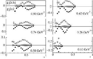
Figure 16: The symmetry between $g_{1}$ and $g_{2}$. (JLab ³He data from E94-010 [275].)

So far, $g_{2}$ DIS data have been discussed. Many data at $W<2$ GeV and $6\times 10^{-3}<Q^{2}<3.3$ GeV² also exist. Being derived using OPE, the Wandzura-Wilczek relation, Eq. (60), should not apply there. Yet, it is instructive to compare $g_{2}$ and $g_{2}^{WW}$ in this region. (In fact, it was done when $d_{2}(Q^{2})$ was discussed, since $d_{2}=\int x^{2}[g_{2}-g_{2}^{WW}]dx$.) Proton and deuteron $g_{2}$ data are available from the RSS experiment at $\left\langle Q^{2}\right\rangle=1.3$ GeV² and for $0.3\leq x_{Bj}\leq 0.8$ [277, 278]. The $x_{Bj}$-dependences of $g_{2}$ and $g_{2}^{WW*}$ (the ^∗ means it is formed using $g_{1}$ measured by RSS and thus is not leading twist) are similar except that generally $|g_{2}^{p}|<|g_{2}^{WW*,p}|$, while $|g_{2}^{n}|>|g_{2}^{WW*,n}|$. The inequality indicates either higher-twist effects or coherent resonance contributions. The ranks and types of the higher-twists are unclear since $g_{2}^{WW*}$ itself contains higher-twists whereas its OPE expression is twist 2. A similar study on $g_{2}^{{}^{3}He}$ from E97-110 [287] was done for $6\times 10^{-3}<Q^{2}<0.3$ GeV². Again, $g_{2}^{{}^{3}He}$ is close to $g_{2}^{WW*,^{3}He}$. Their difference may come from higher-twists or coherence effects, but now also possibly from nuclear effects. Resonance data on $g_{2}^{{}^{3}He}$ are also available from E01-012 [285] and were compared to $g_{2}^{WW,^{3}He}$ computed at leading-twist. It results that $g_{2}^{WW,^{3}He}$ provides an accurate approximation of $g_{2}^{{}^{3}He}$, maybe facilitated by the smearing of resonances in nuclei. Such analysis amounts to assessing the size of twist-3 and higher in $g_{2}$, neglecting structures due to resonances. It also tests hadron-parton spin-duality for ³He, see Section 6.10.

A feature of the $g_{1}$ and $g_{2}$ resonance data is the symmetry around 0 of their $x_{Bj}$-behavior, see Fig. 16. It is observed for the proton [277] and for ³He [275, 284, 285, 287]. DIS data do not display the symmetry. It arises from the smallness of ${\sigma}_{LT}^{\prime}$: since ${\sigma}_{LT}^{\prime}\propto(g_{1}+g_{2})$, then $g_{1}\approx-g_{2}$. In particular, for the $\Delta(1232)~{}3/2^{+}$, ${\sigma}_{LT}^{\prime}\approx 0$ because the dipole component $M_{1+}$ dominates the nucleon-$\Delta$ transition. This holds at low $Q^{2}$ where $M_{1+}\gg E_{1+}$ and $S_{1+}$. At larger $Q^{2}$, another reason arises: resonances being at high $x_{Bj}$, $\int_{x_{Bj}}^{1}(g_{1}/y)dy$ in Eq. (60) is negligible and since $g_{2}^{WW}\approx g_{2}$, then $g_{2}\approx-g_{1}$.

6.10 Study of the hadron-parton spin duality

Hadron-parton duality is the observation that a structure function in the DIS appears as a precise average of its measurement in the resonance domain. This coincidence can be understood as a dearth of dynamical higher-twists. Duality is thus related to the study of parton correlations. In the last two decades precise data were gathered to test duality on $g_{1}$. Duality on $g_{1}^{p}$, $g_{1}^{n}$, $g_{1}^{d}$ and $g_{1}^{{}^{3}He}$ has been studied using the SLAC and JLab data from E143 [268], E154 [256, 269], E155 [257, 270], E94010 [275], E97-103 [284], E99-117 [283], E01-012 [285, 286] (which was dedicated to studying spin-duality), EG1b [279, 280, 281, 282] and RSS  [277, 278]. The $x_{Bj}$-value at which duality appears depends on $Q^{2}$. At low $Q^{2}$, duality is violated around the $\Delta(1232)~{}3/2^{+}$. This is expected since there, $g_{1}<0$ due to the $M_{1+}$ transition dominance; see discussions about $\sigma_{TT}$ on page 6.4 and about the $g_{1}$ and $g_{2}$ symmetry page 16. (The discussion applies to $g_{1}$ because $\sigma_{TT}\propto(g_{1}-\gamma^{2}g_{2})\approx g_{1}(1+\gamma^{2})\propto g_{1}$ at the $\Delta(1232)~{}3/2^{+}$.) Above $Q^{2}=1.2$ GeV² duality seems to be valid at all $x_{Bj}$. Duality’s onset for $g_{1}^{d}$ and $g_{1}^{{}^{3}He}$ appears at smaller $Q^{2}$ than for $g_{1}^{p}$ as expected, since duality is aided by the nucleon Fermi motion inside a composite nucleus.

Spin-duality was also studied using the $A_{1}$ and $A_{2}$ asymmetries using the SLAC, HERMES  [381] and JLab data. Duality in $A_{1}$ arises for $Q^{2}\gtrsim 2.6$ GeV². At lower $Q^{2}$, it is invalidated by the $\Delta(1232)~{}3/2^{+}$. The $A_{1}^{{}^{3}He}$ $Q^{2}$-dependence is weak for both DIS and resonances (except near the $\Delta(1232)~{}3/2^{+}$). This is expected in DIS since $A_{1}\approx g_{1}/F_{1}$ and $g_{1}$ and $F_{1}$ have the same $Q^{2}$-dependence at LO of DGLAP and leading-twist. The weak $Q^{2}$-dependence in the resonances signals duality. Duality in $A_{1}$ seems to arise at greater $Q^{2}$ than for $g_{1}$. Duality in $A_{2}$ arises at lower $Q^{2}$ than for $A_{1}$ because the $\Delta(1232)~{}3/2^{+}$ is suppressed in $A_{2}$, since $A_{2}\propto\sigma_{LT}^{\prime}$.

The similar $Q^{2}$- and $x_{Bj}$-dependences of the DIS and resonance structure functions discussed so far is called “local duality”. “Global duality” considers the moments. It is tested by forming the partial moments $\widetilde{\Gamma}^{res}$ integrated only over the resonances. They are compared to $\widetilde{\Gamma}^{DIS}$ moments covering the same $x_{Bj}$ interval and formed using leading-twist structure functions. $\widetilde{\Gamma}^{DIS}$ is corrected for pQCD radiation and kinematical twists. Global duality has been tested on $\widetilde{\Gamma}_{1}^{p}$ and $\widetilde{\Gamma}_{1}^{d}$ [281], and on $\widetilde{\Gamma}_{1}^{n}$ and $\widetilde{\Gamma}_{1}^{{}^{3}\textnormal{He}}$ [285]. For the proton, duality arises for $Q^{2}\gtrsim 1.8$ GeV² or $Q^{2}\gtrsim 1.0$ GeV² if the elastic reaction is included. For the deuteron, ³He and neutron (extracted from the previous nuclei), duality arises earlier, as expected from Fermi motion.

6.11 Nucleon spin structure at high energy

In this section we will discuss the picture of the nucleon spin structure painted by both high-energy experiments and theory. The PDFs quoted here are for the proton. The neutron PDFs should be nearly identical after SU(2) isospin symmetry rotation.

6.11.1 General conclusions

The polarized inclusive DIS experiments from SLAC, CERN and DESY laid the foundation for our understanding of the nucleon spin structure and showed that:

$\bullet$ The strong force is well described by pQCD, even when spin degrees of freedom are accounted for. Since QCD is the accepted paradigm, the contribution of inclusive, doubly polarized DIS experiments to nucleon spin studies provided an important test of the theory. For example, the verification of the Bjorken sum rule, Eq. (54), has played a central role. To emphasize this, one can recall the oft-quoted statement of Bjorken [382]: “Polarization data has often been the graveyard of fashionable theories. If theorists had their way, they might well ban such measurements altogether out of self-protection.”

$\bullet$ QCD’s fundamental quanta, the quarks and gluons, and their OAM should generate the nucleon spin, see Eq. (31):

$$\vspace{-0.15cm}J=\frac{1}{2}=\frac{1}{2}\Delta\Sigma+\mbox{L}_{q}+\Delta G+\mbox{L}_{g}$$

Estimates for each of the components are discussed in the next Section. Recent determinations suggest $\Delta\Sigma\approx 0.30(5)$, $\mbox{L}_{q}\approx 0.2(1)$, and $\Delta G+\mbox{L}_{g}\approx 0.15(10)$ at $Q^{2}=4$ GeV². Thus the nucleon spin is shared between the three components, with the quark OAM possibly the largest contribution. This result includes the PDF evolution effects from the low $Q^{2}$ nonperturbative domain to the experimental resolution at $Q^{2}=4$ GeV².

$\bullet$ The PDFs extracted from diverse DIS data and evolved to the same $Q^{2}$ are generally consistent. Global analyses show that the up quark polarization in the proton is large and positive, $\Delta\Sigma_{u}\approx 0.85$, whereas the down quark one is smaller and negative, $\Delta\Sigma_{d}\approx-0.43$. The $x_{Bj}$-dependences of $\Delta u+\Delta\overline{u}$ and $\Delta d+\Delta\overline{d}$ are well determined in the kinematical domains of the experiment.

$\bullet$ The gluon axial anomaly [250] is small and cannot explain the “spin crisis”.

$\bullet$ The contribution of the gluon spin, which is only indirectly accessible in inclusive experiments, seems to be moderate.

$\bullet$ Quark OAM, which is required in the baryon LFWF to have nonzero Pauli form factor and anomalous magnetic moment [63], is the most difficult component to measure from DIS; however, an analysis of DIS data at high-$x_{Bj}$, GPD data, as well as LGT suggest it is a major contribution to $J$.

$\bullet$ The Ellis-Jaffe sum rule, Eq. (53), is violated for both nucleons. This either implies a large $\Delta s$, large SU(3)_f breaking effects, or an inaccurate value of $a_{8}$ [152]. Global fits indicate $\Delta s\approx-0.05(5)$, which is too small to fully explain the violation.

$\bullet$ Higher-twist power-suppressed contributions are small at $Q^{2}>1$ GeV².

6.11.2 Individual contributions to the nucleon spin

Total quark spin contribution

The most precise determinations of $\Delta\Sigma$ are from global fits, see Table 3 in the Appendix. In average, $\Delta\Sigma\approx 0.30(5)$. A selection of LGT results is shown in Table 4. The early calculations typically did not include the disconnected diagrams that are responsible for the sea quark contribution. They account for the larger uncertainty in some recent LGT analyses and reduce the predicted $\Delta\Sigma$ by about 30% [189, 383]. (An earlier result indicated only a 5% reduction, but this was evaluated with $m_{\pi}=0.47$ GeV [384]). The determination of $\Delta\Sigma$ from SIDIS at COMPASS [324] agrees with the inclusive data [272]. The two analyses have similar statistical precision.

Individual quark spin contributions

Inclusive DIS data on proton, neutron, and deuteron targets can be used to separate the contributions from different quark polarizations assuming SU(3)_f validity. SIDIS, which tags the struck quark allows the identification of individual quark spin contributions without this assumption. However, the domain where PDFs can be safely extracted assuming factorizations demands a larger momentum scale than untagged DIS. It is presently unclear whether the kinematical range of available data has reached this domain.

Tables 5 and 6 list $\Delta q$ from experiments, models and results from LGT. Overall, $\Delta\Sigma_{u}\approx 0.85$ and $\Delta\Sigma_{d}\approx-0.43$. $\Delta s$ is of special interest since it could explain the violation of the Ellis-Jaffe sum rule (Eq. (53)), and also underlines the limitations of constituent quark models. Ref. [385] reviewed recently the nucleon sea, including $\Delta s$. The current favored value for $\Delta s,$ approximately $-0.05(5)$, is barely enough to reconcile the Ellis-Jaffe sum rule, which predicts $\Delta\Sigma^{EJ}=0.58(12)$ without $\Delta s,$ with the measured $\Delta\Sigma\approx 0.30(5)$. Recent LGT data yield an even smaller $\Delta s$ value, about $-0.03(1)$. (Early quenched LGT data yielded a larger $\Delta s=0.2(1)$, agreeing with the EMC initial determination.) Thus, this suggests that SU(3)_f breaking also contributes to the Ellis-Jaffe sum rule violation [152]. This conclusion is supported by recent global analyses from DSSV [315], NNPDF14 [317] and in particular JAM [319]. Nevertheless, this question remains open since for example, LGT investigations of hyperon axial couplings show no evidence of SU(3)_f violation [386].

There is also tension between the values for $\Delta s$ derived from DIS and from kaon SIDIS data. Those suggest that the $x_{Bj}$-dependence of $\Delta s+\Delta\overline{s}$ flips sign and thus contributes less to $J$ than indicated by DIS data. For example, COMPASS obtains $\Delta s+\Delta\overline{s}=-0.01\pm 0.01$(stat) $\pm 0.01$(syst) from SIDIS whereas a PDF fit of inclusive asymmetries yields $\Delta s+\Delta\overline{s}=-0.08\pm 0.01$(stat) $\pm 0.02$(syst), in clear disagreement. This suggests that even at the large CERN energies, we may not yet be in the factorization domain for SIDIS. Furthermore, a LSS analysis showed that the SIDIS $\Delta s$ is very sensitive to the parameterization of the fragmentation functions and that the lack of their precise knowledge may cause the tension [387]. However, the JAM analysis recently suggested [319] that the tension comes from imposing SU(3)_f, which is consistent with the likely explanation of the Ellis-Jaffe sum rule violation  [152, 388]. The JAM analysis, done at NLO and in the $\overline{MS}$ scheme, was aimed at determining $\Delta s+\Delta\overline{s}(x_{Bj})$ with minimal bias. It used DIS, SIDIS and $e^{+}e^{-}$ annihilation data without imposing SU(3)_f, and allowed for higher-twist contributions. It finds $\Delta s+\Delta\overline{s}=-0.03\pm 0.10$ at $Q^{2}=5$ GeV². Fragmentation function data from LHC, COMPASS, HERMES, BELLE and BaBar may clarify the situation. Measurements of $\overrightarrow{p}p\to\overrightarrow{\Lambda}X$ may also help since the $\Lambda$ polarization depends on $\Delta s$. Reactions utilizing parity violation are also useful: proton strange form factor data, together with neutrino scattering data yield $g_{A}^{s}=\Delta s+\Delta\overline{s}=-0.30\pm 0.42$ [389]. New parity violation data on $g_{A}^{s}$ should be available soon [390] and can be complemented with measurements using the future SoLID detector at JLab  [365]. A polarized ³He target and unpolarized electron beam can provide $g_{1}^{\gamma Z,n}$ and $g_{5}^{\gamma Z,n}$ from $Z^{0}$–$\gamma$ parity-violating interference. These measurements, combined with the existing $g_{1}^{p}$ and $g_{1}^{n}$ data, can determine $\Delta s$ without assuming SU(3)_f [391].

The $x_{Bj}$-dependence of $\Delta u$ and $\Delta d$ can be obtained from $A_{1}\approx g_{1}/F_{1}$ at high $x_{Bj}$ (see Section 6.3.1) and from SIDIS at lower $x_{Bj}$. At high $x_{Bj}$, sea quarks contribute little so $F_{1}$ and $g_{1}$ mostly depend on $u^{+}$, $u^{-}$, $d^{+}$ and $d^{-}$ (see Eqs. (21) and (23)). They can thus be extracted from $F_{1}^{p}$, $F_{1}^{n}$, $g_{1}^{p}$ and $g_{1}^{n}$ assuming isospin symmetry. The results for $\Delta u/u$ and $\Delta d/d$ extracted from $A_{1}$ [279, 283, 291, 392] are shown in Fig. 17. For clarity, only the most precise data are plotted. Smaller $x_{Bj}$ points are from SIDIS data [393]. Global fits are also shown [304, 314, 315, 317]. The latter Ref. used the high-$x_{Bj}$ pQCD constraints discussed in Section 6.3.1 and assumed no quark OAM. OAM is included in the results from Refs. [150, 314].

The $\Delta d/d$ data are negative, agreeing with most models but not with pQCD evolution which predicts that $\Delta d/d>0$ for $x_{Bj}\gtrsim 0.5$ without quark OAM. Including OAM pushes the zero crossing to $x_{Bj}\approx 0.75$, which agrees with the data. PQCD’s validity being established, this suggests that quark OAM is important. Integrating $\Delta u(x_{Bj})$ and $\Delta d(x_{Bj})$ over $x_{Bj}$ yield a large positive $\Delta u$ and a moderate negative $\Delta d$.

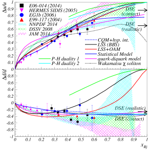
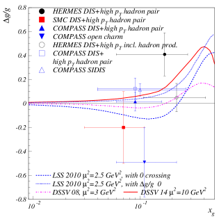
Figure 17: Data and global fits for $\Delta q/q$ vs quark momentum fraction $x_{Bj}$ (left), and for $\Delta g/g$ vs the gluon momentum fraction $x_{g}$ (right).

First results on $\Delta u-\Delta d$ from LGT are becoming available [202, 394].

The $\Delta\overline{u}-\Delta\overline{d}$ difference

Global fits and LGT calculations indicate a nonzero total polarized sea difference $\Delta\overline{u}-\Delta\overline{d}$. (We use the term “sea difference” rather than the conventional “sea asymmetry” in order to avoid confusion with spin asymmetry, a central object of this review.) Ref. [385] recently reviewed the nucleon sea content, including its polarization. An unpolarized non-zero sea difference $\overline{u}-\overline{d}\approx-0.12$ has been known since the early 1990s [128, 130]. Such phenomenon must be nonperturbative since the perturbative process $g\to q\bar{q}$ generating sea quarks is nearly symmetric, and Pauli blocking for $g\to u\bar{u}$ in the proton ($g\to d\bar{d}$ in the neutron) is expected to be very small. Many of the nonperturbative processes proposed for $\overline{u}-\overline{d}\neq 0$ also predict $\Delta\overline{u}-\Delta\overline{d}\neq 0$. As mentioned, $\overline{u}-\overline{d}$ may be related to the total OAM, see Eq. (34). Table 7 provides data and predictions for $\Delta\overline{u}-\Delta\overline{d}$. Other predictions are provided in Refs. [395].

Spin from intrinsic heavy-quarks

More generally, the nonperturbative contribution to the nucleon spin arising from its “intrinsic” heavy quark Fock states – intrinsic strangeness, charm, and bottom [396] – is an interesting question. Such contributions arise from $Q\bar{Q}$ pairs which are multiply connected to the valence quarks. One can show from the OPE that the probability of heavy quark Fock states such as $|uudQ\bar{Q}\rangle$ in the proton scales as $1/M^{2}_{Q}$  [396, 397]. In the case of Abelian theory, a Fock state such as $|e^{+}e^{-}L\bar{L}\rangle$ in positronium atoms arises from the heavy lepton loop light-by-light insertion in the self-energy of positronium. In the Abelian case the probability scales as $1/M^{4}_{L}$. The proton spin $J^{z}$ can receive contributions from the spin $S^{z}$ of the heavy quarks in the $|uudQ\bar{Q}\rangle$ Fock state. For example, the least off-shell hadronic contribution to the $|uuds\bar{s}\rangle$ Fock state has a dual representation as a $|K^{+}(u\bar{s})\Lambda(uds)\rangle$ fluctuation where the polarization of the $\Lambda$ hyperon is opposite to the proton spin $J^{z}$ [117]. Since the spin of the $s$ quark is aligned with $\Lambda$ spin, the $s$ quark will have spin $S^{z}_{s}$ opposite to the proton $J^{z}$. The $\bar{s}$ in the $K^{+}$ is unaligned. Similarly, the spin $S^{z}_{c}$ of the intrinsic charm quark from the $|D^{+}(u\bar{c})\Lambda_{c}(udc)\rangle$ fluctuation of the proton will also be anti-aligned to the proton spin. The magnitude of the spin correlation of the intrinsic Q quark with the proton is thus bounded by the $|uudQ\bar{Q}\rangle$ Fock state probability. The net spin correlation of the intrinsic heavy quarks can be bounded using the OPE [398]. It is also of interest to consider the intrinsic heavy quark distributions of nuclei. For example, as shown in Ref. [399], the gluon and intrinsic heavy quark content of the deuteron will be enhanced due its “hidden-color” degrees of freedom [171, 400], such as $|(uud)_{8_{C}}(ddu)_{8_{C}}\rangle$.

The gluon contribution to the proton spin

$\Delta g/g(x_{Bj})$ and $\Delta g(x_{Bj})$ have been determined from either global fits to $g_{1}$ data via the sensitivity introduced by the DGLAP equations, or from more direct semi-exclusive processes. Tables 8 and 9 summarize the current information on $\Delta G$ and $\Delta G+\mbox{L}_{g}$. Results on $\Delta g/g$ are shown in Fig. 17. The averaged value is $\Delta g/g=0.113\pm 0.038$(stat)$\pm 0.035$(syst).

Orbital angular momenta

Of all the nucleon spin components, the OAMs are the hardest to measure. Quark OAM can be extracted via the GPDs $E$ and $H$, see Eq. (33), the two-parton twist 3 GPD $G_{2}$, see Eq. (35), or GTMDs. They can also be assessed using TMDs with nucleon structure models [49]. While GPDs yield the kinematical OAM, GTMDs provide the canonical definition, see Section 3.1.11. GPD and GTMD measurements are difficult and, in order to obtain the OAM, must be extensive since sum rule analyses are required. The present dearth of data can be alleviated by models if the data are sufficiently constraining so that the model dependence is minimal. See Refs. [401, 139] for examples of such work. In Ref. [401], a model is used to connect $E$ and the Sivers TMD. The fit to the single-spin transverse asymmetries allows to extract the TMD, to which $E$ is connected and then used to extracted $J_{q}$. Thus $L_{q}=J_{q}-\Delta q/2$ can be obtained. In Ref. [139], the quark OAM is computed within a bag model using Eq. (35). A LF analysis of the deuteron single-spin transverse asymmetry [324] also constrains OAM and suggests a small value for $\mbox{L}_{g}$ [402]. Similar conclusions are reached using measurements of the $pp^{\uparrow}\to\pi^{0}X$ single spin transverse asymmetry [403]. LGT can predict $L_{q}$ by calculating $J_{q}$ and subtracting the computed or experimentally known $\Delta q/2$. $\mbox{L}_{g}$ is obtained likewise. Alternatively, a first direct LGT calculation of quark OAMs obtained from the cross-product of position and momentum is outlined in [198]. Quark OAMs are obtained from GTMDs [53, 134, 68] and can be set to follow the canonical $l_{q}$ or kinematical $L_{q}$ OAM definition, or any definition in between by varying the shape of the Wilson link chosen for the calculation. $l_{q}$ and $L_{q}$ can be compared, as well as how they transform into each other, and it is found that $l_{q}>L_{q}$.

Early LGT calculations, which indicated small $L_{q}$ values, did not include the contributions of disconnected diagrams. More recent calculations including the disconnected diagrams yield larger values for the quark OAM, in agreement with several observations: A) The predictions from LF at first order and the Skyrme model that in the nonperturbative domain, the spin of the nucleon comes entirely from the quark OAM, see Section 4.4. B) The relativistic quark model which predicts $l_{q}\approx 0.2$ [110, 111]; C) The $\Delta d/d$ high-$x_{Bj}$ data that is understood within pQCD only if the quark OAM is sizeable [150], see Section 6.3.1; and D) A non-zero nucleon anomalous magnetic moment implies a non-zero quark OAM [63, 64]. Although $L_{q}$ is dominated by disconnected diagrams in LGT, they are absent in the LF and quark models, and highly suppressed for the large-$x_{Bj}$ data. Thus, although the various approaches agree that the quark OAM is important, the underlying mechanisms are evidently different.

Tables 10 and 11 provide the LGT results and the indirect phenomenological determinations from single spin asymmetries. If only the quark OAM or quark total angular momenta are provided in a reference, we have computed the other one assuming $\Delta u/2=0.41(2)$, $\Delta d/2=-0.22(2)$ and $\Delta s/2=-0.05(5)$. One notices on the tables that the strange quark OAM seems to be of opposite sign to $\Delta s$, effectively suppressing the total strange quark contribution to the nucleon spin.

6.11.3 High-energy picture of the nucleon spin structure

The contributions to $J$ listed in Tables 3-11 are shown on Fig. 18. It allows for a visualization of the evolution of our knowledge.

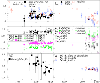
Figure 18: History of the measurements, models and LGT results on $\Delta\Sigma/2$ (top left panel); L (top right panel); $(\Delta q+\Delta\bar{q})/2$ (middle left panel); quark OAM for light flavors (middle right panel); $\Delta G$ (bottom left panel); and $\Delta G+\mbox{L}_{g}$ (bottom right panel). The results shown, from Tables 3-11, are not comprehensive. The determinations of L use different definitions, and may thus not be directly comparable, see Section. 3.1.11. The data points are significantly correlated since they use the same data set and/or related assumptions and/or similar approximations, e.g., quench approximation or neglecting disconnected diagrams for the earlier LGT results. Values were LO-evolved to $Q^{2}=4$ GeV². The uncertainties, when available, were not evolved.

While the measured $\Delta u+\Delta\overline{u}$ agrees with the relativistic quark model, its prediction for $\Delta d+\Delta\overline{d}$ is 50% smaller than the data. Thus the failure of the relativistic quark model stems in part from neglecting the sea quarks, chiefly $\Delta\overline{d}$ and $\Delta s$ to a lesser extent. The situation for the quark OAM is still unclear due the data scarcity. The indication that $\mbox{L}_{s}$ and $\Delta s$ have opposite signs reduces the overall strange quark contribution to $J$ to a second-order effect. Finally, $\Delta G+\mbox{L}_{g}$ appears to be of moderate size and thus not as important as initially thought.

The picture of the nucleon spin structure arising from these high-energy results is as follows: The nucleon appears as a mixture of quasi-free quarks and bremsstrahlung-created gluons, which in turn generate sea quarks. At $Q^{2}\sim 4$ GeV², the valence quarks carry between 30% to 40% of $J$. The sea quarks contribute a smaller value and have opposite sign – about $-10\%$; it is dominated by $\Delta\bar{d}$. The gluons carry about 20% to 40% of $J$. The remainder, up to  50%, comes from the quark OAM. This agrees with the asymptotic prediction $L_{q}\to\Delta\Sigma(Q_{0})+\frac{3n_{f}}{32+6n_{f}}$, assuming $Q_{0}\approx$  1 GeV for the DGLAP evolution starting scale. This, together with the LFHQCD first order prediction that the spin of the nucleon comes entirely from the quark OAM, and hence $\Delta\Sigma(Q_{0})=0$ yields $L_{q}\xrightarrow[Q^{2}\to\infty]{~{}}0.52\,J$ at LO. Part of this physics can be understood as a relativistic effect, the consequence of the Dirac equation for light quarks in a confining potential. In the constituent quark model, this effect is about $0.3\,J$.

Finally, DIS experiments indicate small higher-twist contributions, i.e., power-law suppressed contributions from parton correlations such as quark-quark interactions, even though the lower $Q$ values of the SLAC or HERMES experiments are of the GeV order, close to the $\kappa\approx 0.5$ GeV confinement scale [226]. This is surprising since such correlations are related to quark confinement. (We refer to $\kappa$ rather than $\Lambda_{s}$ which is renormalization scheme dependent and hence ambiguous. Typically $0.3<\Lambda_{s}<1$ GeV [91].)

6.11.4 Pending Questions

The polarized DIS experiments leave several important questions open:

$\bullet$ Why is scale invariance precocious (i.e., why are higher-twist effects small)?

$\bullet$ What are precisely the values of $\Delta G$, $\mbox{L}_{q}$ and $\mbox{L}_{g}$?

$\bullet$ What are the values and roles of parton correlations (higher-twists), and their connection to strong-QCD phenomena such as confinement and hadronic degrees of freedom?

$\bullet$ Is the nucleon simpler to understand at high $x_{Bj}$?

$\bullet$ How does the transverse momentum influence the nucleon spin structure?

$\bullet$ What is the behavior of the polarized PDFs at small $x_{Bj}$?

Except for the two last points, recent inclusive data at lower energy have partially addressed these questions, as will be discussed below. Experiments which measure GPDs and GTMDs are relevant to all of these questions, except for the last point which can be addressed by future polarized EIC experiments.

6.11.5 Contributions from lower energy data

The information gained from low energy experiments includes parton correlations, the high-$x_{Bj}$ domain of structure functions, the various contributions to the nucleon spin, the transition between the hadronic and partonic degrees of freedom, and tests of nucleon structure models.

$\bullet$ Parton correlations: Overall higher-twist leads only to small deviations from Bjorken scaling even at $Q^{2}\approx 1$ GeV². In fact, the low-$Q^{2}$ data allow us to quantify the characteristic scale $Q_{0}$ at which leading-twist pQCD fails, see Section 7. In the $\overline{MS}$ scheme and N⁴LO, $Q_{0}\approx 0.75$ GeV. Individual higher-twist contributions, however, can be significant. For example, for $\Gamma_{1}(Q^{2}=1$ GeV${}^{2})$ $f_{2}$ (twist 4) has similar strength as $\Gamma_{1}^{\mbox{\scriptsize{twist~{}2}}}$. The overall smallness of the total higher-twist effect comes from the sign alternation of the $Q^{2-twist}$ series and the similar magnitude of its coefficients near $Q^{2}=1$ GeV².

$\bullet$ The $x_{Bj}$-dependence of the effect of parton correlations has been determined for $g_{1}$; the dynamical higher-twist contribution was found to be significant at moderate $x_{Bj}$ but becomes less important at high and low $x_{Bj}$. Since $g_{1}$ is itself small at high $x_{Bj}$, higher-twists remain important there. This conclusion can agree with the absence of large higher-twist contribution in $g_{1}^{n}$ for $Q^{2}\sim 1$ GeV² (Fig. 15), if kinematical higher-twist contribution cancels the dynamical contribution.

$\bullet$ The verification of the Burkhardt-Cottingham sum rule, Eq. (50), implies that $g_{2}$ is not singular. This should apply to each term of the $g_{2}$ twist series.

$\bullet$ At $Q^{2}<1$ GeV², higher-twist effects become noticeable: For example, at $Q^{2}=0.6$ GeV², their contribution to $g_{2}^{n}$ appears to be similar to the twist-2 term contributing to $g_{2}^{WW}$ (Fig. 15), although uncertainties remain important.

The indications that the overall higher-twist contributions are under control allow one to extend the database used to extract the polarized PDFs [305, 313, 320].

High-$x_{Bj}$ data

Measurements from JLab experiments have provided the first significant constraints on polarized PDFs at high $x_{Bj}$. Valence quark dominance is confirmed.

Information on the nucleon spin components

The data at high $x_{Bj}$ have constrained $\Delta\Sigma$, the quark OAM and $\Delta G$. For example, in the global analysis of Ref. [305], the uncertainty on $\Delta G$ has decreased by a factor of 2 at $x_{Bj}=0.3$ and by a factor of 4 at $x_{Bj}=0.5$. Furthermore, these data have revealed the importance of the quark OAM. However, to reliably obtain its value, the quark wave functions of the nucleon have to be known for all $x_{Bj}$, rather than only at high $x_{Bj}$.

Fits of the $\Gamma_{1}$ data at $Q^{2}>1$ GeV² indicate $\Delta\Sigma^{p}=0.15\pm 0.07$ and $\Delta\Sigma^{n}=0.35\pm 0.08$. This difference suggests an insufficient knowledge $g_{1}$ at low $x_{Bj}$, rather than a breaking of isospin symmetry.

The transition between partonic and hadronic descriptions

At large $Q^{2}$, data and pQCD predictions agree well without the need to account for parton correlations; this is at first surprising, but it can be understood in terms of higher-twist contributions of alternating signs. At intermediate $Q^{2}$, the transition between descriptions based on partonic versus hadronic descriptions of the strong force such as the $\chi$PT approach, is characterized by a marked $Q^{2}$-evolution for most moments. However, the evolution is smooth e.g., without indication of phase transition, an important fact in the context of Section 7. At lower $Q^{2}$, $\chi$PT predictions initially disagreed with most of the data for structure function moments. Recent calculations agree better, but some challenges remain for $\chi$PT. New LGT methods are being developed which should allow tractable, reliable first principle calculations of PDFs.

Neutron information

Constraints on neutron structure extracted from experiments using deuteron and ³He targets appear to be consistent; this validates the use of light nuclei as effective polarized neutron targets in the $Q^{2}$ range of the data. These results provide complementary checks on nuclear effects: such effects are small ($\approx 10\%$) for ³He due to the near cancelation between proton spins, but nuclear corrections are difficult to compute since the ³He nucleus is tightly bound. Conversely, the corrections are large ($\approx 50\%$) for the deuteron but more computationally tractable because the deuteron is a weakly bound $n-p$ object.

7 Perspectives: Unexpected connections

Studying nucleon structure is fundamental since nucleons represent most of the known matter. It provides primary information on the strong force and the confinement of quarks and gluons. We provide here an example of what has been learned from doubly polarized inclusive experiments at moderate $Q^{2}$ from JLab. These experiments determined the $Q^{2}$-dependence of spin observables and thus constrained the connections between partonic and hadronic degrees of freedom. A goal of these experiments was to motivate new nonperturbative theoretical approaches and insights into understanding nonperturbative QCD. We discuss here how this goal was achieved.

As discussed at the end of the previous Section, the data at the transition between the perturbative and nonperturbative-QCD domains evolve smoothly. A dramatic behavior could have been expected from the pole structure of the perturbative running coupling; $\alpha_{s}\xrightarrow[Q\to\Lambda_{s}]{}\infty$. However, this Landau pole is unphysical and only signals the breakdown of pQCD [91] rather than the actual behavior of $\alpha_{s}$. In contrast, a smooth behavior is observed e.g. for the Bjorken sum $\Gamma_{1}^{p-n}$, see Fig. 12. At low $Q^{2}$, $\Gamma_{1}^{p-n}$ is effectively $Q^{2}$-independent, i.e., QCD’s approximate conformal behavior seen at large $Q^{2}$ (Bjorken scaling) is recovered at low $Q^{2}$ (see Section 4.3.2). This permits us to use the AdS/CFT correspondence [216] an incarnation of which is the LFHQCD framework [35], see Section 4.4, which predicts that $\Gamma_{1}^{p-n}(Q^{2})=\big{(}1-e^{-\frac{Q^{2}}{4\kappa^{2}}}\big{)}/6$ [357]. Data [373] and LFHQCD prediction agree well; see Fig. 12. Remarkably, the prediction has no adjustable parameters since $\kappa$ is fixed by hadron masses (in Fig. 12, $\kappa=M_{\rho}/\sqrt{2}$).

The LFHQCD prediction is valid up to $Q^{2}\approx 1$ GeV². At higher $Q^{2}$, gluonic corrections not included in LFHQCD become important. However, there pQCD’s Eq. (55) may be applied. The validity domains of LFHQCD and pQCD overlap around $Q^{2}\approx 1$ GeV²; matching the magnitude and the first derivative of their predictions allows one to relate the pQCD parameter $\Lambda_{s}$ to the LFHQCD parameter $\kappa$ or equivalently to hadronic masses [157]. For example, in ${\overline{MS}}$ scheme at LO, $\Lambda_{\overline{MS}}=M_{\rho}e^{-a}/\sqrt{a},$ where $a=4\big{(}\sqrt{\ln(2)^{2}+1+\beta_{0}/4}-\ln(2)\big{)}/\beta_{0}$. For $n_{f}=3$ quark flavors, $a\approx 0.55$.

The $\rho$ meson is the ground-state solution of the quark-antiquark LFHQCD Schrödinger equation including the spin-spin interaction [226, 404], i.e., the solution with radial excitation $n=0$ and internal OAM $L=0$ and $S=1$. Higher mass mesons are described with $n>0$ or/and $L>0$. They are shown in Fig. 19. The baryon spectrum can be obtained similarly or via the mass symmetry between baryons and mesons using superconformal algebra [225].

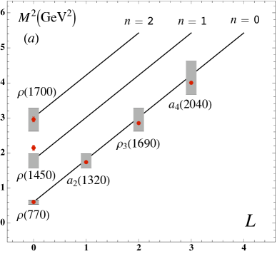
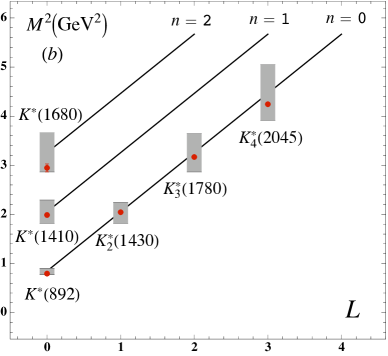
Figure 19: The mass spectrum for unflavored (a) and strange light vector mesons (b) predicted by LFHQCD using only $\Lambda_{s}$ as input [156] . The gray bands provide the uncertainty. The points indicate the experimental values.

Computing the hadron spectrum from $\Lambda_{s}$, such as shown in Fig. 19, has been a long-thought goal of the strong force studies. LFHQCD is not QCD but it represents a semiclassical approximation that successfully incorporates basic aspects of QCD’s nonperturbative dynamics that are not explicit from its Lagrangian. Those include confinement and the emergence of a related mass scale, universal Regge trajectories, and a massless pion in the chiral limit [405]. The confinement potential is determined by implementing QCD’s conformal symmetry, following de Alfaro, Fubini and Furlan who showed how a mass scale can be introduced in the Hamiltonian without affecting the action conformal invariance [227, 228]. The potential is also related by LFHQCD to a dilaton-modified representation of the conformal group in AdS₅ space, Thus, the connection of the hadron mass spectrum [156] to key results derived from the QCD Bjorken sum rule represents an exciting progress toward long-sought goals of physics, and it provides an example of how spin studies foster progress in our understanding of fundamental physics. Another profound connection relates the holographic structure of form factors (and unpolarized quark distributions), which depends on the number of components of a bound state, to the properties of the Regge trajectory of the vector meson that couples to the quark current in a given hadron [97, 223]. This procedure incorporates axial currents and the axial-vector meson spectrum to describe axial form factors and the structure of polarized quark distributions in the LFHQCD approach [406].

8 Outlook

We reviewed in Section 6 the constraints on the composition of nucleon spin which have been obtained from existing doubly polarized inclusive data. In Section 7, we gave an example of the exciting advances obtained from these data. In this section we will discuss constraints which can be obtained from presently scheduled future spin experiments. Most of these experiments are dedicated to measurements of GPDs and TMDs, which now provide the main avenue for spin structure studies.

JLab’s upcoming experimental studies will utilize the upgrade of the electron beam energy from 6 to 12 GeV. The upgraded JLab retains its high polarized luminosity (several $10^{36}$ cm^-2s^-1) which will allow larger kinematic coverage of the DIS region. In particular, higher values of $x_{Bj}$ will be reached, allowing for $\Delta u/u$ and $\Delta d/d$ measurements up to $x_{Bj}\approx 0.8$ for $W>2$ GeV. The quark OAM analysis discussed in Section 6.11.2 will thus be improved. Three such experiments have been approved for running: one on neutron utilizing a ³He target in JLab Hall A, one in Hall B on proton and neutron (Deuteron) targets, and the third one, planned in Hall C with a neutron (³He) target [343], is scheduled to run very soon (2019).

The large solid angle detector CLAS12 [407] in Hall B is well suited to measure $\Gamma_{1}$ up to $Q^{2}=$ 6 GeV² and to minimize the low-$x_{Bj}$ uncertainties at the values of $Q^{2}$ reached at 6 GeV. These data will also refine the determination of higher twists. In addition, inclusive data from CLAS12 will significantly constrain the polarized PDFs of the nucleons [305]: the precision on $\Delta G$ extracted from lepton DIS via DGLAP analysis is expected to improve by a factor of 3 at moderate and low $x_{Bj}$. It will complement the $\Delta G$ measurements from p-p reactions at RHIC. The precision on $\Delta u$ and $\Delta d$ will improve by a factor of 2. Knowledge of $\Delta s$ will be less improved since the inclusive data only give weak constraints. Constrains on $\Delta s$ can be obtained in Hall A using the SoLID [365] experiment without assuming SU(3)_f symmetry [391]. Measurements of $\Delta G$ at RHIC are expected to continue for another decade using the upgraded STAR and sPHENIX detectors [408], until the advent of the electron-ion collider (EIC) [327].

The GPDs are among the most important quantities to be measured at the upgraded JLab [409, 410]. A first experiment has already taken most of its data [409]. Since at $Q^{2}$ of a few GeV², $L_{q}$ appears to be the largest contribution to the nucleon spin, the JLab GPD program is clearly crucial. Information on the quark OAM will also be provided by measurements of the nucleon GTMDs on polarized H, D and ³He targets [411] utilizing the Hall A and B SIDIS experimental programs.

The ongoing SIDIS and Drell-Yan measurements which access TMDs are expected to continue at CERN using the COMPASS phase-III upgrade. TMDs can also be measured with the upgraded STAR and sPHENIX detectors at RHIC [408]. Spin experiments are also possible at the LHC with polarized nucleon and nuclear targets using the proposed fixed-target facility AFTER@LHC [412].

Precise DIS data are lacking at $x_{Bj}\lesssim 0.05$ (see e.g., the DSSV14 global fit [318]). The proposed EIC can access this domain with a luminosity of up to $10^{34}$ cm^-2s^-1. It will allow for traditional polarized DIS, DDIS, SIDIS, exclusive and charged current ($W^{+/-}$) DIS measurements. Precise inclusive data over a much extended $x_{Bj}$ range will yield $\Delta G$ with increased precision from DGLAP global fits. The discrepancy between $\Delta\Sigma^{p}$ and $\Delta\Sigma^{n}$ (Section 6.9.1), which is most likely due to the paucity of low-$x_{Bj}$ data, should thus be clarified. Furthermore, the tension between the $\Delta s$ from DIS and SIDIS can be solved by DIS charged current charm production with a high-luminosity collider such as the EIC. Charged current DIS will allow for flavor separation at high $Q^{2}$ and a first glance at the $g_{5}^{\gamma Z,n}$ structure function [15].

Other future facilities for nucleon spin structure studies are NICA (Nuclotron-based Ion Collider Facilities) at JINR in Dubna [413], and possibly an EIC in China (EIC@HIAF). The NICA collider at Dubna was approved in 2008; it will provide polarized proton and deuteron beams up to $\sqrt{s}=27$ GeV. These beams will allow polarized Drell-Yan studies of TMDs and direct photon production which can access $\Delta G$. China’s HIAF (High Intensity Heavy Ion Accelerator Facility) was approved in 2015. EIC@HIAF, the facility relevant to nucleon spin studies, is not yet approved as of 2018. The EIC@HIAF collider would provide a 3 GeV polarized electron beam colliding with 15 GeV polarized protons. It would measure $\Delta s$, $\overline{\Delta u}-\overline{\Delta d}$, GPDs and TMDs over $0.01\leq x_{Bj}\leq 0.2$ with a luminosity of about $5\times 10^{32}$ cm^-2s^-1. Improvements of the polarized sources, beams, and targets are proceeding at these facilities.

The success of the constituent quark model in the early days of QCD suggested a simple picture for the origin of the nucleon spin: it was expected to come from the quark spins, $\Delta\Sigma=1$. However, the first nucleon spin structure experiments, in particular EMC, showed that the nucleon spin composition is far from being trivial. This complexity means that spin degrees of freedom reveal interesting information on the nucleon structure and on the strong force nonperturbative mechanisms. The next experimental step was the verification of the Bjorken sum rule, thereby verifying that QCD is valid even when spin degrees of freedom are involved. The inclusive programs of SLAC, CERN and DESY also provided a mapping of the $x_{Bj}$ and $Q^{2}$ dependences of the $g_{1}$ structure function, yielding knowledge on the quark polarized distributions $\Delta q(x_{Bj})$ and some constraints on the gluon spin distribution $\Delta G$ and on higher twists. The main goal of the subsequent JLab program was to study how partonic degrees of freedom merge to produce hadronic systems. These data have led to advances that permit an analytic computation of the hadron mass spectrum with $\Lambda_{s}$ as the sole input. Such a calculation represents exciting progress toward reaching the long-sought and primary goals of strong force studies. The measurements and theoretical understanding discussed in this review, which has been focused on doubly-polarized inclusive observables, have provided testimony on the importance and dynamism of studies of the spin structure of the nucleon. The future prospects discussed here show that this research remains as dynamic as it was in the aftermath of the historical EMC measurement.

Acknowledgments

The authors thank S. Širca and R. S. Sufian for their useful comments on the manuscript. This review is based in part upon work supported by the U.S. Department of Energy, the Office of Science, and the Office of Nuclear Physics under contract DE-AC05-06OR23177. This work is also supported by the Department of Energy contract DE–AC02–76SF00515.

Appendix. Tables of the contributions to the nucleon spin

Ref.	$Q^{2}$ (GeV2)	$\Delta\Sigma$	Remarks
-	-	1	naive quark model
[110]	-	0.75$\pm$0.05	relativistic quark model
[108]	-	0.58$\pm 0.12$	Ellis-Jaffe SR
[107]	-	0.60	quark parton model
[114]	10.7	0.14$\pm$0.23	EMC
[110]	10.7	0.01$\pm$0.29	EMC (Jaffe-manohar analysis)
[414]	-	0.30	Skyrme model
[415]	-	$0.09$	Instanton model
[271]	10	0.28$\pm$0.16	SMC
[255]	-	0.41$\pm 0.05$	global analysis
[268]	3	0.33$\pm$0.06	E143
[33]	10	0.31$\pm$0.07	BBS
[416]	-	0.37	$\chi$ quark model
[299]	1	0.5$\pm$0.1	global fit
[124]	4	0.168	GRSV 1995
[267]	2	0.39$\pm$0.11	E142
[256]	5	0.20$\pm$0.08	E154
[302]	4	0.342	LSS 1997
[417]	-	$0.4$	relativistic quark model
[300]	1	0.45$\pm$0.10	ABFR 1998
[309]	5	0.26$\pm$0.02	AAC 2000
[257]	5	0.23$\pm$0.07	E155
[316]	5	0.197 0.273	Standard GRSV 2000 SU(3)f breaking
[336]	4	0.282	Stat. model
[304]	1	0.21$\pm$0.10	LSS 2001
[301]	4	0.198	ABFR 2001
[418]	5	0.16$\pm$0.08	Global analysis
[375]	4	0.298	BB 2002
[310]	5	0.213$\pm$0.138	AAC 2003
[367]	5	0.35$\pm$0.08	Neutron (3He) data (Section 6.9.1)
[282]	5	0.169$\pm$0.084	Proton data (Section 6.9.1)
[419]	-	0.366	$\chi$ quark soliton model
[420, 125]	$\infty$	$0.33$	chiral quark soliton model. $n_{f}=6$
[311]	5	0.26$\pm$0.09	AAC 2006
[274]	5	0.330$\pm$0.039	HERMES Glob. fit
[272]	10	0.35$\pm$0.06	COMPASS
[312]	5	0.245$\pm$0.06	AAC 2008
[152]	$\approx 0.2$	0.39	cloudy bag model w/ SU(3)f breaking
[315]	4	0.245	DSSV08
[306]	4	0.231$\pm$65	LSS 2010
[308]	4	0.193$\pm$75	BB 2010
[126]	$\approx 0.2$	$0.23\pm 0.01$	Gauge-invariant cloudy bag model
[82]	4	0.18$\pm$0.20	NNPDF 2013
[317]	10	0.18$\pm$0.21	NNPDF 2014
[132]	-	0.72$\pm$0.04	unquenched quark mod.
[35]	5	0.30	LFHQCD
[421]	3	$0.31\pm 0.08$	$\chi$ effective $\mathcal{L}$ model
[422]	-	0.308	LFHQCD
[323]	3	0.32$\pm$0.07	COMPASS 2017 deuteron data
[361]	5	0.28$\pm$0.04	JAM 2016
[334]	$\approx 1$	0.602	chiral quark model
[320]	5	0.285	KTA17 global fit
[48]	1	0.17	AdS/QCD q-qq model
[319]	5	0.36$\pm$0.09	JAM 2017

Table 3: Determinations of $\Delta\Sigma$ from experiments and models. Experimental results, including global fits, are in bold and are given in the $\overline{MS}$ scheme. The model list is indicative rather than comprehensive.

Ref.	$Q^{2}$ (GeV2)	$\Delta\Sigma$	Remarks
[423]	-	$0.18\pm 0.02$	Altmeyer, Gockeler et al. Quenched calc.
[424]	-	$0.18\pm 0.10$	Fukugita et al. Quenched calc. w/ $\chi$ extrap.
[425]	-	$0.25\pm 0.12$	U. Kentucky group. Quenched calc. w/ $\chi$ extrap.
[190]	2	$0.59\pm 0.07$	Gockeler et al. u,d only. Quenched calc. w/ $\chi$ extrap.
[426]	3	$0.26\pm 0.12$	U. Kentucky group. Quenched calc. w/ $\chi$ extrap.
[427]	5	$0.20\pm 0.12$	SESAM 1999. $\chi$ extrap. Unspecified RS
[193]	4	$0.682\pm 0.18$	LHPC 2003. u, d only. $\chi$ extrap.
[428]	4	$0.60\pm 0.02$	QCDSF 2003. u, d only. Quenched calc. w/ $\chi$ extrap.
[429]	4	$0.402\pm 0.048$	QCDSF-UKQCD 2007. u, d only. $\chi$ extrap.
[430]	5	$0.42\pm 0.02$	LHPC. u, d only. $\chi$ extrap.
[431]	7.4	$0.448\pm 0.037$	QCDSF 2011. $m_{\pi}$=285 MeV. Partly quenched calc.
[432]	4	$0.296\pm 0.010$	Twisted-Mass 2011 u, d only. W/ $\chi$ extrap.
[433]	4	0.606$\pm$0.052	Twisted-Mass 2013 u, d only. $m_{\pi}$=213 MeV
[434]	4	0.507$\pm$0.008	Twisted-Mass 2013. Phys. q masses
[435]	4	$0.25\pm 0.12$	$\chi$QCD 2013. Quenched calc. w/ $\chi$ extrap.
[436]	4	$0.400\pm 0.035$	Twisted-Mass 2016. Phys. $\pi$ mass
[189]	4	0.398$\pm 0.031$	Twisted-Mass 2017. Phys. $\pi$ mass
[437]	4	$0.494\pm 0.019$	Partly quenched calc. $m_{\pi}=317$ MeV

Table 4: Continuation of Table 3, for LGT results. They are given in the $\overline{MS}$ scheme unless stated otherwise. The list is not comprehensive.

Ref.	$Q^{2}$ (GeV2)	$\Delta u+\Delta\overline{u}$	$\Delta d+\Delta\overline{d}$	$\Delta s+\Delta\overline{s}$	Remarks
-	-	4/3	-1/3	0	quark model
[110]	-	0.86	-0.22	0	relat. q. mod.
[114]	10	0.74(10)	-0.54(10)	-0.20(11)	EMC
[414]	-	0.78	-0.48	0	Skyrme model
[438]	-	-	-	-0.03	$g_{a}^{s}$ SU(3) skyrme model
[415]	-	0.867	-0.216	-	Instanton model
[271]	10	0.82(5)	-0.44(5)	-0.10(5)	SMC
[268]	3	0.84(2)	-0.42(2)	-0.09(5)	E143
[33]	10	0.83(3)	-0.43(3)	-0.10(3)	BBS
[416]	-	0.79	-0.32	-0.10	$\chi$ quark model
[124]	4	0.914	-0.338	-0.068	GRSV 1995
[267]	2	-	-	-0.06(6)	E142
[256]	5	0.69${}^{(15)}_{(5)}$	-0.40${}^{(8)}_{(5)}$	-0.02${}^{(1)}_{(4)}$	E154
[302]	4	0.839	-0.405	-0.079	LSS 1997
[273]	5	0.842(13)	-0.427(13)	-0.085(18)	HERMES (1997)
[417]	-	0.75	-0.48	-0.07	relat. quark model
[309]	5	0.812	-0.462	-0.118(74)	AAC 2000 global fit
[257]	5	0.95	-0.42	0.01	E155
[316]	5	0.795 0.774	-0.470 -0.493	-0.128 -0.006	Standard GRSV 2000 SU(3)f breaking
[336]	4	0.714	-0.344	-0.088	Stat. model
[304]	1	0.80(3)	-0.47(5)	-0.13(4)	LSS 2001
[301]	4	0.692	-0.418	-0.081	ABFR 2001
[375]	4	0.854(66)	-0.413(104)	-0.143(34)	BB 2002
[439]	-	-	-	-0.0052(15)	$g_{a}^{s}$ chiral quark model
[310]	5	-	-	-0.124(46)	AAC 2003
[440]	-	-	-	- 0.05(2)	$g_{a}^{s}$ pentaquark model
[419]	-	0.814	-0.362	-0.086	$\chi$ quark soliton model
[311]	5	-	-	-0.12(4)	AAC 2006
[272]	10	-	-	-0.08(3)	COMPASS
[274]	5	0.842(13)	-0.427(13)	-0.085(18)	HERMES Glob. fit
[389]	-	-	-	-0.30(42)	PV + $\nu$ data
[152]	-	0.84(2)	-0.43(2)	-0.02(2)	cloudy bag model w/ SU(3)f breaking
[315]	4	0.814	-0.456	-0.056	DSSV08
[306]	4	-	-	-0.118(20)	LSS 2010
[308]	4	0.866(0)	-0.404(0)	-0.118(20)	BB 2010
[53]	-	0.996	-0.248	-	LC const. quark mod.
[53]	-	1.148	-0.286	-	LC $\chi$ qu. solit. mod.
[126]	$\approx 0.2$	$0.38\pm 0.01$	$-0.15\pm 0.01$	-	Gauge-invariant cloudy bag model
[82]	1	0.80(8)	-0.46(8)	-0.13(9)	NNPDF 2013
[317]	10	0.79(7)	-0.47(7)	-0.07(7)	NNPDF (2014)
[132]	-	1.10(3)	-0.38(1)	0	unquenched quark mod.
[421]	$\approx 0.5$	0.90(3)	-0.38(3)	-0.07(${}^{4}_{7}$)	$\chi$ effective $\mathcal{L}$ model
[323]	3	0.84(2)	-0.44(2)	-0.10(2)	D COMPASS
[49]	1	0.606	-0.002	-	LF quark mod.
[361]	1	0.83(1)	-0.44(1)	-0.10(1)	JAM16
[320]	5	0.926	-0.341	-	KTA16 global fit
[334]	$\approx 1$	1.024	-0.398	-0.023	chiral quark model
[52]	-	1.892	0.792	-	AdS/QCD q-qq model
[48]	1	0.71(9)	-0.54${}^{19}_{13}$	-	AdS/QCD q-qq model
[319]	5	-	-	-0.03(10)	JAM17

Table 5: Same as Table 3 but for $\Delta q$. Results are ordered chronologically. The list for models is indicative rather than comprehensive.

Ref.	$Q^{2}$ (GeV2)	$\Delta u+\Delta\overline{u}$	$\Delta d+\Delta\overline{d}$	$\Delta s+\Delta\overline{s}$	Remarks
[424]	-	0.638(54)	-0.347(46)	-0.0109(30)	Fukugita et al. Quenched calc. w/ $\chi$ extrap.
[425]	-	0.79(11)	-0.42(11)	-0.12(1)	U. Kentucky group. Quenched calc. w/ $\chi$ extrap.
[190]	2	0.830(70)	-0.244(22)	-	Gockeler et al. u,d only. Quenched calc. w/ $\chi$ extrap.
[426]	3	-	-	-0.116(12)	U. Kentucky group. Quenched calc. w/ $\chi$ extrap.
[427]	5	0.62(7)	-0.29(6)	-0.12(7)	SESAM 1999. $\chi$ extrap. Unspecified RS
[428]	4	0.84(2)	-0.24(2)	-	QCDSF 2003. u, d only. Quenched calc. w/ $\chi$ extrap.
[441]	-	-	-	-0.019(11)	Unrenormalized result. W/ $\chi$ extrap.
[430]	5	0.822(72)	-0.406(70)	-	LHPC 2010. u, d only. $\chi$ extrap.
[431]	7.4	0.787(18)	-0.319(15)	-0.020(10)	QCDSF 2011. $m_{\pi}$=285 MeV. Partly quenched calc.
[432]	4	0.610(14)	-0.314(10)	-	Twisted-Mass 2011 u, d only. W/ $\chi$ extrap.
[434]	4	0.820(11)	-0.313(11)	-0.023(34)	Twisted-Mass 2013. Phys. q masses
[433]	4	0.886(48)	-0.280(32)	-	Twisted-Mass 2013 u, d only. $m_{\pi}$=213 MeV
[435]	4	0.79(16)	-0.36(15)	-0.12(1)	$\chi$QCD 2013. Quenched calc. w/ $\chi$ extrap.
[436]	4	0.828(32)	-0.387(20)	-0.042(10)	Twisted-Mass 2016. Phys. $\pi$ mass
[189]	4	0.826(26)	-0.386(14)	-0.042(10)	Twisted-Mass 2017. Phys. $\pi$ mass
[437]	4	0.863(17)	-0.345(11)	-0.0240(24)	Partly quenched calc. $m_{\pi}=317$ MeV

Table 6: Continuation of Table 5, for LGT results. They are given in the $\overline{MS}$ scheme unless stated otherwise. The list is not comprehensive.

Ref.	$Q^{2}$ (GeV2)	$\Delta\overline{u}-\Delta\overline{d}$	$\Delta\overline{u}$	$\Delta\overline{d}$	Remarks
[442]	-	0	0	0	$\pi$-cloud model
[415]	4	0.215	-	-	Instanton model
[443]	2	0.014(13)	-	-	$\rho$-cloud model
[444]	10	0.00(19)	0.01(6)	0.01(18)	SMC
[445]	4	0.76(1)	-	-	cloud model, $\rho$-$\pi$ interf.
[446]	-	0.31	-	-	$\chi$ soliton model
[393]	2.5	0.01(6)	-0.01(4)	-0.02(5)	HERMES
[316]	5	0 0.32	-0.064 0.085	-0.064 -0.235	Standard GRSV 2000 SU(3)f breaking
[447]	4	0.023(31)	-	-	meson cloud bag model
[448]	-	0.2	-	-	Instanton model
[336]	4	0.12	0.046	-0.087	Stat. model
[449]	-	0.2	-	-	sea model with Pauli-blocking
[450]	1	0.12	-	-	cloud model $\sigma$-$\pi$ interf.
[392]	2.5	0.048(64)	-0.002(23)	-0.054(35)	HERMES
[451]	10	0.00(5)	-	-	COMPASS
[315]	5	0.15	0.036	-0.114	DSSV08
[321]	3	-0.04(3)	-	-	COMPASS
[322]	3	0.06(5)	0.02(2)	-0.05(4)	COMPASS
[317]	10	0.17(8)	0.06(6)	-0.11(6)	NNPDF (2014)
[452] [453]	-	-	$>0$	-	0.05$<x_{Bj}<$0.2. STAR and PHENIX $W^{\pm}$, $Z$ prod.
[319]	5	0.05(8)	-	-	global fit (JAM 2017)
[200]	4	0.24(6)	-	-	$m_{\pi}$=310 MeV

Table 7: Phenomenological (top) and LGT (bottom) results on the sea asymmetry $\Delta\overline{u}-\Delta\overline{d}$. Results are in the $\overline{MS}$ scheme. The lists for models and LGT are ordered chronologically and are not comprehensive.

Ref.	$Q^{2}$ (GeV2)	Contribution	Remarks
[271]	5	$\Delta G$=0.9(6)	SMC incl. DGLAP
[33]	1	$\Delta G$=0.5	BBS global fit
[299]	1	$\Delta G$=1.5(8)	Ball et al. global fit
[124]	4	$\Delta G$=1.44	GRSV 1995
[256]	5	$\Delta G$=0.9(5)	E154 incl. DGLAP
[300]	1	$\Delta G$=1.5(9)	ABFR 1998
[309]	5	$\Delta G$=0.920(2334)	AAC 2000
[454]	2	$\Delta g/g$=0.41(18) at $\left\langle x_{g}\right\rangle$= 0.17	HERMES DIS+high-$p_{T}$ hadron pairs
[257]	5	$\Delta G$=0.8(7)	E155 incl. DGLAP
[316]	5	$\Delta G$=0.708 $\Delta G=0.974$	Standard GRSV 2000 SU(3)f breaking
[304]	1	$\Delta G$=0.68(32)	LSS 2001
[301]	4	$\Delta G=1.262$	ABFR 2001
[375]	4	$\Delta G=0.931(669)$	BB2002
[310]	5	$\Delta G=0.861(2185)$	AAC 2003
[455]	13	$\Delta g/g$=-0.20(30) at $\left\langle x_{g}\right\rangle=0.07$	SMC DIS+high-$p_{T}$ hadron pairs
[456]	4	$\Delta G+\mbox{L}_{g}=0.40(5)$	Valence only. GPD constrained w/ nucl. form factors
[457]	2	$\Delta G+\mbox{L}_{g}=0.22$	GPD model
[458]	3	$\Delta g/g$=0.016(79) at $\left\langle x_{g}\right\rangle=0.09$	COMPASS quasi-real high-$p_{T}$ hadron pairs prod.
[311]	5	$\Delta G=0.67(186)$	AAC 2006
[459] [460]	1.9	$\Delta G+\mbox{L}_{g}$=0.23(27)	JLab and HERMES DVCS data
[420] [125]	$\infty$	$\Delta G+\mbox{L}_{g}=0.264$	$\chi$ quark solit. mod. $n_{f}=6$
[312]	5	$\Delta G=1.07(104)$	AAC 2008
[115], [154]	4	$\Delta G+\mbox{L}_{g}=0.208(63)$	quark model w/ pion cloud
[461]	4	$\Delta G+\mbox{L}_{g}=0.20(7)$	GPD model
[462]	13	$\Delta g/g$=-0.49(29) at $\left\langle x_{g}\right\rangle$ = 0.11	COMPASS Open Charm
[315]	5	$\Delta G$=-0.073	DSSV08
[463]	1.35	$\Delta g/g=0.049(35)(^{126}_{~{}99})$ at $\left\langle x_{g}\right\rangle$ = 0.22	HERMES DIS + high-$p_{T}$ incl. hadron production
[131]	-	$\Delta G+\mbox{L}_{g}=0.163(28)$	quark model+unpol. sea asym. (Garvey relation)
[306]	4	$\Delta G=-0.02(34)$	LSS 2010
[308]	4	$\Delta G=0.462(430)$	BB 2010
[126]	$\approx 0.2$	$\Delta G+\mbox{L}_{g}=-0.26(10)$	Gauge-invariant cloudy bag model
[401]	4	$\Delta G+\mbox{L}_{g}=0.23(3)$	single spin trans. asy.
[464]	5	$\Delta G\lesssim 0.4$	c-quark axial-charge constraint
[465]	13	$\Delta g/g$=-0.13(21) at $\left\langle x_{g}\right\rangle$= 0.2	COMPASS open charm
[465]	3	$\Delta G$=0.24(9)	Global fit+COMPASS open charm
[104]	4	$\Delta G+\mbox{L}_{g}=0.263(107)$	GPD constrained w/ nucl. form factors
[466]	3	$\Delta g/g$=0.125(87) at $\left\langle x_{g}\right\rangle$=0.09	COMPASS DIS + high-$p_{T}$ hadron pairs
[82]	4	$\Delta G=-0.9(39)$	NNPDF 2013
[467]	4	$\Delta G+\mbox{L}_{g}=0.274(29)$	GPD constrained w/ nucl. form factors
[132]	-	$\Delta G+\mbox{L}_{g}=0.14(7)$	unquenched quark model
[35]	5	$\Delta G+\mbox{L}_{g}=0.09$	LFHQCD
[318]	10	$\int_{0.001}^{1}\Delta gdx$=0.37(59)	DSSV14
[468]	10	$\Delta G$=0.21(10)	NNPDF [317] including STAR data
[469]	3	$\Delta g/g$=0.113(52) at $\left\langle x_{g}\right\rangle$= 0.1	COMPASS SIDIS deuteron data
[49]	1	$\Delta G+\mbox{L}_{g}=0.152$	LF quark model
[320]	5	$\Delta G$=0.391	KTA17 global fit
[334]	$\approx 1$	$\Delta G+\mbox{L}_{g}=0$	chiral quark model
[52]	-	$\Delta G+\mbox{L}_{g}=-0.035$	AdS/QCD scalar quark-diquark model

Table 8: Same as Table 3 but for gluon contributions. $x_{g}$ is the gluon momentum fraction. Results are in the $\overline{MS}$ scheme. The lists for models and LGT are ordered chronologically and are not comprehensive.

Ref.	$Q^{2}$ (GeV2)	$\Delta G+\mbox{L}_{g}$	Remarks
[426]	3	0.20(7)	U. Kentucky group. Quenched calc. w/ $\chi$ extrap.
[428]	4	0.17(7)	QCDSF 2003. u, d only. Quenched calc. w/ $\chi$ extrap.
[470]	4	0.249(12)	CC$\chi$PT. u, d only. W/ $\chi$ extrap.
[429]	4	0.274(11)	QCDSF-UKQCD. u, d only. $\chi$ extrap.
[430]	5	0.262(18)	LHPC 2010. u, d only. $\chi$ extrap.
[432]	4	0.358(40)	Twisted-Mass 2011 u, d only. W/ $\chi$ extrap.
[433]	4	0.289(32)	Twisted-Mass 2013 u, d only. $m_{\pi}$=0.213 GeV
[434]	4	0.220(110)	Twisted-Mass 2013. Phys. q masses
[435]	4	0.14(4)	$\chi$QCD col. w/ $\chi$ extrap.
[436]	4	0.325(25)	Twisted-Mass 2016. Phys. $\pi$ mass
[203]	10	0.251(47)	$\chi$QCD 2017. Phys. $\pi$ mass
[189]	4	0.09(6)	Twisted-Mass 2017. Phys. $\pi$ mass

Table 9: Continuation of Table 8, for LGT results. They are given in the $\overline{MS}$ scheme.

Ref.	$Q^{2}$ (GeV2)	$\mbox{L}_{u}$ $J_{u}$	$\mbox{L}_{d}$ $J_{d}$	$\mbox{L}_{s}$ $J_{s}$	disc. diag.?	Remarks
[107]	-	$\hskip 85.35826pt\mbox{L}_{q}=0.20$			N/A	quark parton model
[110] [154]	-	0.46 0.89	-0.11 -0.22	0 0	N/A	relat. quark model Canonical def.
[416]	-	$\hskip 85.35826pt\mbox{L}_{q}=0.32$			N/A	$\chi$ quark model
[316]	5	$\mbox{L}_{q+g}=0.18$                                      $\mbox{L}_{q+g}=0.08$				Standard GRSV 2000 SU(3)f breaking
[457]	2	-0.12(2) 0.29	0.20(2) -0.03	0.07(5) 0.02	N/A	GPD model
[456]	4	-0.26(1) 0.15(3)	0.17(3) -0.05(4)	- -	Valence contr. only	GPD constrained w/ nucl. form factors
[420] [125]	$\infty$	$L_{u+d}=0.050$ $J_{u+d}=0.236$			Valence contr. only	$\chi$ quark solit. mod. $n_{f}=6$
[115], [154]	4	-0.005(60) 0.405(57)	0.107(33) -0.113(26)	- -	N/A	quark model w/ pion cloud
[459] [460]	1.9	-0.03(23) 0.38(23)	0.11(15) -0.11(15)	- -	N/A	JLab and HERMES DVCS data
[461]	4	-0.17(4) 0.24(3)	0.24(3) 0.02(3)	0.07(6) 0.02(3)	N/A	GPD model
[131]	-	$l_{u+d+s}=0.147(27)$ $J_{u+d+s}=0.337(28)$			N/A	quark model+unpol. sea asym. (Garvey relation)
[126]	$\approx 0.2$	0.34(13) 0.72(14)	0.19(13) 0.04(14)	- -	N/A	Gauge-invariant cloudy bag model
[401]	4	-0.166(15) 0.244(11)	0.235(12) 0.015(6)$(^{20}_{~{}5})$	0.062(${}^{5}_{9}$) 0.012 $(^{2}_{8})$	N/A	single spin trans. asy.
[53]	-	0.071 0.569	0.055 -0.069	- -	N/A	LC constituent quark model
[53]	-	-0.008 0.566	0.077 -0.066	- -	N/A	$\chi$ quark soliton model
[104]	4	-0.12(11) 0.286(107)	0.17(2) -0.049(7)	- -	N/A	GPD constrained w/ nucl. form factors
[467]	4	-0.18(3) $0.230(^{9}_{24})$	0.21(3) $-0.004(^{10}_{16})$	- -	N/A	GPD constrained w/ nucl. form factors
[35]	5	$\mbox{L}_{u+d+s}=0.25$ $J_{u+d+s}=0.31$			N/A	LFHQCD.
[132]	-	$l_{u+d+s}=0.221(41)$, $J_{u+d+s}=0.36(7)$			N/A	unquenched quark model
[49]	1	0.055 0.358	-0.001 -0.010	- -	N/A	LF quark model
[334]	$\approx 1$	0.265 0.777	-0.066 -0.265	0 -0.012	N/A	chiral quark model
[52]	-	-0.3812 0.565	-0.4258 -0.030			AdS/QCD scalar quark-diquark model

Table 10: Phenomenological results on quark $\mbox{L}_{q}=\mbox{L}_{u}+\mbox{L}_{d}+\mbox{L}_{s}$ and total angular momenta $J_{q}=\mbox{L}_{q}+\Delta\Sigma_{q}/2$. Results are in the $\overline{MS}$ scheme. They use different definitions of $\mbox{L}_{q}$, and may thus not be directly comparable, see Section 3.1.11. The list is ordered chronologically and is not comprehensive.

Ref.	$Q^{2}$ (GeV2)	$L_{u}$ $J_{u}$	$L_{d}$ $J_{d}$	$L_{s}$ $J_{s}$	disc. diag.?	Remarks
[426]	3	$L_{u+d+s}=0.17(6)$, $J_{u+d+s}=0.30(7)$			yes	U. Kentucky group. Quenched calc. w/ $\chi$ extrap.
[193]	4	$\hskip 85.35826ptJ_{q}=0.338(4)$			No	LHPC 2003. u, d only. $\chi$ extrap.
[428]	4	-0.05(6) 0.37(6)	0.08(4) -0.04(4)	- -	no	QCDSF. u, d only. Quenched calc. w/ $\chi$ extrap.
[470]	4	-0.14(2) 0.266(9)	0.21(2) -0.015(8)	- -	no	CC$\chi$PT. u, d only. W/ $\chi$ extrap.
[429]	4	-0.18(2) 0.230(8)	0.22(2) -0.004(8)	- -	no	QCDSF-UKQCD. u, d only. $\chi$ extrap.
[430]	5	-0.175(40) 0.236(18)	0.205(35) 0.002(4)	- -	no	LHPC 2010. u, d only. $\chi$ extrap.
[432]	4	-0.141(30) 0.189(29)	0.116(30) -0.047(28)	- -	no	Twisted-Mass 2011 u, d only. W/ $\chi$ extrap.
[433]	4	-0.229(30) 0.214(27)	0.137(30) -0.003(17)	- -	no	Twisted-Mass 2013 u, d only. $m_{\pi}$=0.213 GeV
[435]	4	-0.003(8) 0.37(6)	0.195(8) -0.02(4)	0.07(1) 0.012(4)	yes	$\chi$QCD col. w/ $\chi$ extrap.
[434]	4	-0.208(95) 0.202(78)	0.078 (95) 0.078(78)	- -	yes	Twisted-Mass 2013. Phys. q masses
[436]	4	-0.118(43) 0.296(40)	0.252(41) 0.058(40)	0.067(21) 0.046(20)	yes	Twisted-Mass 2016. Phys. $\pi$ mass
[189]	4	-0.104(29) 0.310(26)	0.249(27) 0.056(26)	0.067(21) 0.046(21)	yes	Twisted-Mass 2017. Phys. $\pi$ mass

Table 11: Same as Table 10 but for LGT results.

Lexicon and acronyms

To make this review more accessible to non-specialists, we provide here specific terms associated with the nucleon structure, with short explanations and links to where they are first discussed in the review. For convenience, we also provide the definitions of the acronyms used in this review.

• AdS/CFT: anti-de-Sitter/conformal field theory.

• AdS/QCD: anti-de-Sitter/quantum chromodynamics.

• anti-de-Sitter (AdS) space: a maximal symmetric space endowed with a constant negative curvature.

• Asymptotic freedom: QCD’s property that its strength decreases at short distances.

• Asymptotic series: see Poincaré series.

• $\beta$-function: the logarithmic derivative of $\alpha_{s}$: $\beta\left(\mu^{2}\right)=\frac{d\alpha_{s}\left(\mu\right)}{d\mbox{\footnotesize{ln}}(\mu)}$ where $\mu$ is the subtraction point. In the perturbative domain, $\beta$ can be expressed as a perturbative series $\beta=-\frac{1}{4\pi}\sum_{n=0}\left(\frac{\alpha_{s}}{4\pi}\right)^{n}\beta_{n}$.

• Balitsky-Fadin-Kuraev-Lipatov (BFKL) evolution equations: the equations controlling the low-$x_{Bj}$ behavior of structure functions.

• BBS: Brodsky-Burkardt-Schmidt.

• BC: Burkhardt-Cottingham.

• BLM: Brodsky-Lepage-Mackenzie. See Principle of Maximal Conformality (PMC).

• CERN: Conseil Européen pour la Recherche Nucléaire.

• $\chi$PT: chiral perturbation theory.

• CEBAF: continuous electron beam accelerator facility.

• CLAS: CEBAF large acceptance spectrometer.

• COMPASS: common muon and proton apparatus for structure and spectroscopy.

• Condensate (or Vacuum Expectation Value, VEV): the vacuum expectation value of a given local operator. Condensates allow one to parameterize the nonperturbative OPE’s power corrections. Condensates and vacuum loop diagrams do not appear in the frame-independent light-front Hamiltonian since all lines have $k^{+}=k^{0}+k^{3}\geq 0$ and the sum of $+$ momenta is conserved at every vertex. In the light-front formalism condensates are associated with physics of the hadron wavefunction and are called “in-hadron” condensates, which refers to physics possibly contained in the higher LF Fock states of the hadrons [471]. In the case of the Higgs theory, the usual Higgs VEV of the instant form Hamiltonian is replaced by a “zero mode”, a background field with $k^{+}=0$ [472].

• Conformal behavior/theory: the behavior of a quantity or a theory that is scale invariant. In a conformal theory the $\beta$-function vanishes. More rigorously, a conformal theory is invariant under both dilatation and the special conformal transformations which involve coordinate inversion.

• Cornwall-Norton moment: the moment $\int_{0}^{1}x^{N}g(x,Q^{2})dx$ of a structure function $g(x_{Bj},Q^{2})$. See Mellin-transform.

• Constituent quarks: unphysical particles of approximately a third of the nucleon mass and ingredients of constituent quark models. They provide the $J^{PC}$ quantum numbers describing the hadron. Constituent quarks can be viewed as valence quarks dressed by virtual pairs of partons.

• DDIS: diffractive deep inelastic scattering.

• DESY: Deutsches Elektronen-Synchrotron.

• Dimensional transmutation: the emergence of a mass or momentum scale in a quantum theory with a classical Lagrangian devoid of explicit mass or energy parameters [473].

• DIS: deep inelastic scattering.

• Distribution amplitudes: universal quantities describing the valence quark structure of hadrons and nuclei.

• Dokshitzer-Gribov-Lipatov-Altarelli-Parisi (DGLAP) evolution equations: the equations controlling the $Q^{2}$ behavior of structure functions, except at extreme $x_{Bj}$ (low- and large-$x_{Bj}$). The DGLAP equations are used in global determinations of parton distributions by evolving the distribution functions from an initial to a final scale.

• DVCS: deeply virtual Compton scattering.

• Effective charge: an effective coupling defined from a perturbatively calculable observable. It includes all perturbative and relevant nonperturbative effects [176].

• Effective coupling: the renormalized (running) coupling, in contrast with the constant unphysical bare coupling.

• EFL: Efremov-Leader-Teryaev.

• Efremov-Radyushkin-Brodsky-Lepage (ERBL) evolution equations: the equations controlling the evolution of the Distribution amplitudes in $\ln(Q^{2})$.

• EIC: electron-ion collider.

• EMC: european muon collaboration.

• Factorization scale: the scale at which nonperturbative effects become negligible.

• Factorization theorem: the ability to separate at short distance the perturbative coupling of the probe to the nucleon, from the nonperturbative nucleon structure [27].

• Freezing: the loss of scale dependence of finite $\alpha_{s}$ in the infrared. See also conformal behavior.

• Gauge link or link variable: in Lattice QCD, the segment(s) linking two lattice sites to which a unitary matrix is associated to implement gauge invariance. While quarks reside at the lattice sites, gauge links effectively represent the gluon field. Closed links are Wilson loops used to construct the LGT Lagrangian.

• GDH: Gerasimov-Drell-Hearn.

• Ghosts: ghosts referred to unphysical fields. For example in certain gauges in QED and QCD, such as the Feynman gauge, there are four vector-boson fields: two transversely polarized bosons (photons and gluons, respectively), a longitudinally polarized one, and a scalar one with a negative metric. This later is referred to as a ghost photon/gluon and is unphysical since it does not represent an independent degree of freedom: While vector-bosons have in principle 4-spin degrees of freedom, only three are independent due to the additional constraint from gauge invariance. In Yang-Mills theories, Faddeev-Popov ghosts are fictitious particles of spin zero but that obey the Fermi–Dirac statistics (negative-metric particles). These characteristics are chosen so that the ghost propagator complements the non-transverse term in the gluon propagator to make it transverse, and thus insure current conservation. In radiation or Coulomb gauge, the scalar and longitudinally polarized vector-bosons are replaced by the Coulomb interaction. Axial gauges where vector-bosons are always transverse, in particular the LC gauge $A^{+}$, can alternatively be used to avoid introducing ghosts.

• GPD: generalized parton distributions.

• GTMD: generalized transverse momentum distributions

• Hard reactions or hard scattering: high-energy processes, in particular in which the quarks are resolved.

• HIAF: high intensity heavy ion accelerator facility.

• Higher-twist: See Twist

• HLFHS: holographic light-front hadron structure collaboration.

• IMF: infinite momentum frame.

• Instant form, or instant time quantization: the traditional second quantization of a field theory, done at instant time $t$; one of the forms of relativistic dynamics introduced by Dirac. See Light-front quantization and Sec. 3.1.3.

• JAM: JLab angular momentum collaboration

• JINR: Joint Institute for Nuclear Research.

• JLab: Jefferson Laboratory.

• Landau pole, Landau singularity or Landau ghost: the point where a perturbative coupling diverges. At first order (1-loop) in pQCD, this occurs at the scale parameter $\Lambda_{s}$. The value can depend on the choice of renormalization scheme, the order $\beta_{i}$ at which the coupling series is estimated, the number of flavors $n_{f}$ and the approximation chosen to solve the QCD $\beta$ equation. The Landau pole is unphysical.

• LC: light cone.

• LEGS: laser electron gamma source.

• LF: light-front.

• LFHQCD: light-front holographic QCD.

• Light-front quantization: second quantizaton of a field theory done at fixed LF-time $\tau$, rather than at instant time $t$; one of the relativistic forms introduced by Dirac. The equal LF-time condition defines a plane, rather than a cone, tangent to the light-cone. Thus the name ”Light-Front”. See Instant form and Sec. 3.1.3.

• LFWF: light-front wave function.

• LGT: lattice gauge theory.

• LO: leading order.

• LSS: Leader-Sidorov-Stamenov.

• LT: longitudinal-transverse.

• MAMI: Mainz Microtron.

• Mellin transform: the moment $\int_{0}^{1}x^{N}g(x,Q^{2})dx$, typically of a structure function $g(x_{Bj},Q^{2})$. It transforms $g(x_{Bj},Q^{2})$ to Mellin space ($N,Q^{2}$), with $N$ the moment’s order. Advantages are 1) that the $Q^{2}$-evolution of moments are simpler than that of structure function $Q^{2}$-evolution, since the nonperturbative $x_{Bj}$-dependence is integrated over. Furthermore, convolutions of PDFs partition functions (see Eqs. (26)–(28)) become simple products in Mellin-space. The structure functions are then recovered by inverse transforming back to the $x_{Bj},Q^{2}$ space; and 2) low-$N$ moments are computable on the lattice with smaller noise than (non-local) structure functions. Structure functions can be obtain by inverse transform the 1- to $N$-moments, if $N$ is large enough.

• NICA: nuclotron-based ion collider facilities.

• NLO: next-to-leading order.

• NNLO: next-to-next-to-leading order.

• OAM: orbital angular momentum.

• Operator Product Expansion (OPE). See also higher-twist: the OPE uses the twist of effective operators to predict the power-law fall-off of an amplitude. It thus can be used to distinguish logarithmic leading twist perturbative corrections from the $1/Q^{n}$ power corrections. The OPE typically does not provide values for the nonperturbative power correction coefficients.

• Optical Theorem: the relation between a cross-section and its corresponding photo-absorption amplitude. Generally speaking, the dispersion of a beam is related to the transition amplitude. This results from the unitarity of a reaction. The theorem expresses the fact that the dispersive part of a process (the cross-section) is proportional to the imaginary part of the transition amplitude. The case is similar to classical optics, where complex refraction indices are introduced to express the dispersion of a beam of light in a medium imperfectly transparent. This explains the name of the theorem.

• PDF: parton distribution functions

• Poincaré series (also Asymptotic series). See also “renormalons”. A series that converges up to an order $k$ and then diverges. The series reaches its best convergence at order $N_{b}$ and then diverges for orders $N\gtrsim N_{b}+\sqrt{N_{b}}$. Quantum Field Theory series typically are asymptotic and converge up to an order $N_{b}\simeq 1/a$, with $a$ the expansion coefficient. IR renormalons generate an $n!\beta^{n}$ factorial growth of the $n$th coefficients in nonconformal ($\beta\neq 0$) theories. Perturbative calculation to high order ($\alpha_{s}^{20}$) has been performed on the lattice [476] to check the asymptotic behavior of QCD series. Factorial growth is seen up to the 20th order of the calculated series.

• Positivity constraint: the requirement on PDF functions that scattering cross-sections must be positive.

• Power corrections. See “Higher-twist” and “Renormalons”.

• pQCD: perturbative quantum chromodynamics.

• Principle of Maximal Conformality (PMC): a method used to set the renormalization scale, order-by-order in perturbation theory, by shifting all $\beta$ terms in the pQCD series into the renormalization scale of the running QCD coupling at each order. The resulting coefficients of the series then match the coefficients of the corresponding conformal theory with $\beta=0$. The PMC generalizes the Brodsky Lepage Mackenzie BLM method to all orders. In the Abelian $N_{C}\to 0$ limit, the PMC reduces to the standard Gell-Mann–Low method used for scale setting in QED [474].

• Pure gauge sector, pure Yang Mills or pure field. Non Abelian field theory without fermions. See also quenched approximation.

• PV: parity violating.

• PWIA: plane wave impulse approximation.

• QCD: quantum chromodynamics.

• QCD counting rules: the asymptotic constraints imposed on form factors and transition amplitudes by the minimum number of partons involved in the elastic scattering.

• QCD scale parameter $\Lambda_{s}$: the UV scale ruling the energy-dependence of $\alpha_{s}$. It also provides the scale at which $\alpha_{s}$ is expected to be large, and nonperturbative treatment of QCD is required [91].

• QED: quantum electrodynamics.

• Quenched approximation: calculations where the fermion loops are neglected. It differs from the pure gauge, pure Yang Mills case in that heavy (static) quarks are present.

• Renormalization scale: the argument of the running coupling. See also “Subtraction point”.

• Renormalon: the residual between the physical value of an observable and the Asymptotic series of the observable at its best convergence order $n\simeq 1/\alpha_{s}$. The terms of a pQCD calculation which involve the $\beta$-function typically diverge as $n!$: i.e., as a renormalon. Borel summation techniques indicate that IR renormalons can often be interpreted as power corrections. Thus, IR renormalons should be related to the higher twist corrections of the OPE formalism [475]. The existence of IR renormalons in pure gauge QCD is supported by lattice QCD [476]. See also “Asymptotic series”.

• RHIC: relativistic heavy ion collider (RHIC).

• RSS: resonance spin structure.

• Sea quarks: quarks stemming from gluon splitting $g\to q\bar{q}$ and from QCD’s vacuum fluctuations. This second contribution is frame dependent and avoided in the light-front formalism. Evidence for sea quarks making up the nucleon structure in addition to the valence quarks came from DIS data yielding PDFs that strongly rise at low-$x_{Bj}$.

• SIDIS: semi-inclusive deep inelastic scattering.

• SLAC: Stanford Linear Accelerator Center.

• SMC: spin muon collaboration.

• SoLID: solenoidal large intensity device.

• SSA: single-spin asymmetry.

• Subtraction point $\mu$: the scale at which the renormalization procedure subtracts the UV divergences.

• Sum rules: a relation between the moment of a structure function, a form factor or a photoabsorption cross-section, and static properties of the nucleon. A more general definition includes relations of moments to double deeply virtual Compton scattering amplitudes rather than to a static property.

• Tadpole corrections: in the context of lattice QCD, tadpole terms are unphysical contributions to the lattice action which arise from the discretization of space-time. They contribute at NLO of the bare coupling $g^{bare}=\sqrt{4\pi\alpha_{s}^{bare}}$ to the expression of the gauge link variable $U_{\overrightarrow{\mu}}$. (The LO corresponds to the continuum limit.) To suppress these contributions, one can redefine the lattice action by adding larger Wilson loops or by rescaling the link variable.

• TMD: transverse momentum distributions.

• TT: transverse-transverse.

• TUNL: Triangle Universities Nuclear Laboratory.

• Twist: the twist $\tau$ of an elementary operator is given by its dimension minus its spin. For example, the quark operator $\psi$ has dimension $3$, spin $1/2$ and thus $\tau=1$. For elastic scattering at high $Q^{2}$, LF QCD gives $\tau=n-1$ with $n$ is the number of effective constituents of a hadron. For DIS, structure functions are dominated by $\tau=2$, the leading-twist. Higher-twist are $Q^{2-\tau}$ power corrections to those, typically derived from the OPE analysis of the nonperturbative effects of multiparton interactions. Higher-twist is sometimes interpretable as kinematical phenomena, e.g. the mass $M$ of a nucleon introduces a power correction beyond the pQCD scaling violations, or as dynamical phenomena, e.g., the intermediate distance transverse forces that confine quarks [38, 39].

• Unitarity: conservation of the probability: the sum of probabilities that a scattering occurs with any reaction, or does not occur, must be 1.

• Unquenched QCD: see pure gauge sector and quenched approximation.

• Valence quarks: the nucleon quark content once all quark-antiquark pairs (sea quarks) are excluded. Valence quarks determine the correct quantum numbers of hadrons.

• VEV: vacuum expectation value.

• VVCS: doubly virtual Compton scattering.

• Wilson line: a Wilson line represents all of the final-state interactions between the struck quark in DIS and the target spectators. It generates both leading and higher twists effects: for example the exchange of a gluon between the struck quark and the proton’s spectators after the quark has been struck yields the Sivers effect [26]. It also contributes to DDIS at leading twist.

• Wilson Loops: closed paths linking various sites in a lattice [183]. They are used to define the lattice action and Tadpole corrections. (See Section 4.2.)

References

- [1] K. Y. J. Chiu and S. J. Brodsky, “Angular momentum conservation law in light-front quantum field theory,” Phys. Rev. D 95, 065035 (2017) [arXiv:1702.01127 [hep-th]].
- [2] X. Ji, J. H. Zhang and Y. Zhao, “Justifying the naive partonic sum rule for proton spin,” Phys. Lett. B 743, 180 (2015) [arXiv:1409.6329 [hep-ph]].
- [3] T. Kinoshita, “Quantum electrodynamics,” Singapore, Singapore: World Scientific (1990) 997 p. (Advanced series on directions in high energy physics, 7)
- [4] S. D. Bass, “The spin structure of the proton,” Rev. Mod. Phys. 77, 1257 (2005) [hep-ph/0411005].
- [5] J. P. Chen, A. Deur and Z. E. Meziani, “Sum rules and moments of the nucleon spin structure functions,” Mod. Phys. Lett. A 20, 2745 (2005) [nucl-ex/0509007].
- [6] M. Burkardt, C. A. Miller and W. D. Nowak, “Spin-polarized high-energy scattering of charged leptons on nucleons,” Rept. Prog. Phys. 73, 016201 (2010) [arXiv:0812.2208 [hep-ph]].
- [7] S. E. Kuhn, J.-P. Chen and E. Leader, “Spin structure of the nucleon – status and recent results,” Prog. Part. Nucl. Phys. 63, 1 (2009) [arXiv:0812.3535 [hep-ph]].
- [8] J. P. Chen, “Moments of spin structure functions: Sum rules and polarizabilities,” Int. J. Mod. Phys. E 19, 1893 (2010) [arXiv:1001.3898 [nucl-ex]].
- [9] C. A. Aidala, S. D. Bass, D. Hasch and G. K. Mallot, “The spin structure of the nucleon,” Rev. Mod. Phys. 85, 655 (2013) [arXiv:1209.2803 [hep-ph]].
- [10] J. Blumlein, “The theory of deeply inelastic scattering,” Prog. Part. Nucl. Phys. 69, 28 (2013) [arXiv:1208.6087 [hep-ph]].
- [11] M. Grosse Perdekamp and F. Yuan, “Transverse spin structure of the nucleon,” Ann. Rev. Nucl. Part. Sci. 65, 429 (2015) [arXiv:1510.06783 [hep-ph]].
- [12] R. L. Jaffe and X. D. Ji, “Chiral odd PDFs and polarized Drell-Yan,” Phys. Rev. Lett. 67, 552 (1991).
- [13] D. J. Gross and F. Wilczek, Ultraviolet behavior of nonabelian gauge theories, Phys. Rev. Lett. 30, 1343 (1973); H. D. Politzer, Reliable perturbative results for strong interactions?, Phys. Rev. Lett. 30, 1346 (1973).
- [14] W. M. Alberico, S. M. Bilenky and C. Maieron, “Strangeness in the nucleon: Neutrino-nucleon and polarized electron-nucleon scattering,” Phys. Rept. 358, 227 (2002) [hep-ph/0102269].
- [15] M. Anselmino, A. Efremov and E. Leader, “The theory and phenomenology of polarized deep inelastic scattering,” Phys. Rept. 261, 1 (1995) [Erratum: Phys. Rept. 281, 399 (1997)] [hep-ph/9501369].
- [16] P. A. M. Guichon and M. Vanderhaeghen, “How to reconcile the Rosenbluth and the polarization transfer method in the measurement of the proton form factors,” Phys. Rev. Lett. 91 (2003) 142303 [hep-ph/0306007].
- [17] F. Gross, “Electromagnetic studies in nuclei,” AIP Conference Proceedings 133, 330 (1985)
- [18] M. Tanabashi et al. [Particle Data Group], “Review of Particle Physics,” Phys. Rev. D 98, 030001 (2018).
- [19] M. N. Rosenbluth, “High energy elastic scattering of electrons on protons,” Phys. Rev. 79, 615 (1950).
- [20] V. D. Burkert and T. S. H. Lee, “Electromagnetic meson production in the nucleon resonance region,” Int. J. Mod. Phys. E 13, 1035 (2004) [nucl-ex/0407020].
- [21] D. Boer, S. J. Brodsky and D. S. Hwang, “Initial-state interactions in the unpolarized Drell-Yan process,” Phys. Rev. D 67, 054003 (2003) [hep-ph/0211110].
- [22] S. J. Brodsky, D. S. Hwang and I. Schmidt, “Final-state interactions and single-spin asymmetries in semi-inclusive deep inelastic scattering,” Phys. Lett. B 530, 99 (2002) [hep-ph/0201296].
- [23] J. C. Collins, “Leading-twist single-transverse-spin asymmetries: Drell-Yan and deep-inelastic scattering,” Phys. Lett. B 536, 43 (2002) [hep-ph/0204004].
- [24] S. J. Brodsky, D. S. Hwang and I. Schmidt, “Initial-state interactions and single-spin asymmetries in Drell-Yan processes,” Nucl. Phys. B 642, 344 (2002) [hep-ph/0206259].
- [25] S. J. Brodsky, D. S. Hwang, Y. V. Kovchegov, I. Schmidt and M. D. Sievert, “Single-spin asymmetries in semi-inclusive deep inelastic scattering and Drell-Yan processes,” Phys. Rev. D 88, 014032 (2013) [arXiv:1304.5237 [hep-ph]].
- [26] D. W. Sivers, “Single-spin production asymmetries from the hard scattering of point-like constituents,” Phys. Rev. D 41, 83 (1990).
- [27] S. B. Libby and G. F. Sterman, “Jet and lepton-pair production in high-energy lepton-hadron and hadron-hadron scattering,” Phys. Rev. D 18, 3252 (1978); R. K. Ellis, H. Georgi, M. Machacek, H. D. Politzer and G. G. Ross, “Factorization and the parton model in QCD,” Phys. Lett. 78B, 281 (1978); “Perturbation theory and the parton model in QCD,” Nucl. Phys. B 152, 285 (1979);
- [28] M. Breidenbach et al., “Observed behavior of highly inelastic electron-proton scattering,” Phys. Rev. Lett. 23, 935 (1969); E. D. Bloom et al., “High-energy inelastic scattering at and ,” Phys. Rev. Lett. 23, 930 (1969).
- [29] J. B. Kogut and D. E. Soper, “ Quantum electrodynamics in the infinite-momentum frame,” Phys. Rev. D 1, 2901 (1970).
- [30] S. J. Brodsky, H. C. Pauli and S. S. Pinsky, “Quantum chromodynamics and other field theories on the light-cone,” Phys. Rept. 301, 299 (1998) [hep-ph/9705477].
- [31] S. J. Brodsky and G. R. Farrar, “Scaling laws at large transverse momentum,” Phys. Rev. Lett. 31, 1153 (1973); “Scaling laws for large-momentum-transfer processes,” Phys. Rev. D 11, 1309 (1975).
- [32] V. A. Matveev, R. M. Muradian and A. N. Tavkhelidze, “Automodellism in the large-angle elastic scattering and structure of hadrons,” Lett. Nuovo Cim. 7, 719 (1973).
- [33] S. J. Brodsky, M. Burkardt and I. Schmidt, “QCD constraints on the shape of polarized quark and gluon distributions,” Nucl. Phys. B 441, 197 (1995) [hep-ph/9401328].
- [34] S. Weinberg, “Dynamics at infinite momentum,” Phys. Rev. 150, 1313 (1966).
- [35] S. J. Brodsky, G. F. de Téramond, H. G. Dosch and J. Erlich, “Light-front holographic QCD and emerging confinement,” Phys. Rept. 584, 1 (2015) [arXiv:1407.8131 [hep-ph]].
- [36] L. D. Faddeev and V. N. Popov, Feynman diagrams for the Yang–Mills field, Phys. Lett. B 25, 29 (1967).
- [37] R. L. Jaffe, “Spin, twist and hadron structure in deep inelastic processes,” hep-ph/9602236.
- [38] M. Burkardt, “Transverse force on quarks in deep-inelastic scattering,” Phys. Rev. D 88, 114502 (2013) [arXiv:0810.3589 [hep-ph]].
- [39] M. Abdallah and M. Burkardt, “Transverse force on transversely polarized quarks in longitudinally polarized nucleons,” Phys. Rev. D 94, 094040 (2016) [arXiv:1610.01166 [hep-ph]].
- [40] B. Q. Ma, I. Schmidt and J. Soffer, “The Quark spin distributions of the nucleon,” Phys. Lett. B 441, 461 (1998) [hep-ph/9710247]; B. Q. Ma, D. Qing and I. Schmidt, “Electromagnetic form factors of nucleons in a light-cone diquark model,” Phys. Rev. C 65, 035205 (2002) [hep-ph/0202015]; B. Pasquini, S. Cazzaniga and S. Boffi, “Transverse momentum dependent PDFs in a light-cone quark model,” Phys. Rev. D 78, 034025 (2008) [arXiv:0806.2298 [hep-ph]]; A. Bacchetta, F. Conti and M. Radici, “Transverse-momentum distributions in a diquark spectator model,” Phys. Rev. D 78, 074010 (2008) [arXiv:0807.0323 [hep-ph]]; A. Courtoy, S. Scopetta and V. Vento, “Analyzing the Boer-Mulders function within different quark models,” Phys. Rev. D 80, 074032 (2009) [arXiv:0909.1404 [hep-ph]];
- [41] T. Gutsche, V. E. Lyubovitskij, I. Schmidt and A. Vega, “Light-front quark model consistent with Drell-Yan-West duality and quark counting rules,” Phys. Rev. D 89, 054033 (2014) [Erratum: Phys. Rev. D 92, 019902 (2015)] [arXiv:1306.0366 [hep-ph]]; “Nucleon structure in a light-front quark model consistent with quark counting rules and data,” Phys. Rev. D 91, 054028 (2015) [arXiv:1411.1710 [hep-ph]]; “Pion light-front wavefunction, PDF and the electromagnetic form factor,” J. Phys. G 42, 095005 (2015) [arXiv:1410.6424 [hep-ph]];
- [42] T. Maji, C. Mondal, D. Chakrabarti and O. V. Teryaev, “Relating transverse structure of various PDFs,” JHEP 1601, 165 (2016) [arXiv:1506.04560 [hep-ph]].
- [43] T. Liu and B. Q. Ma, “Quark Wigner distributions in a light-cone spectator model,” Phys. Rev. D 91, 034019 (2015) [arXiv:1501.07690 [hep-ph]].
- [44] C. Lorcé, B. Pasquini, X. Xiong and F. Yuan, “The quark orbital angular momentum from Wigner distributions and light-cone wavefunctions,” Phys. Rev. D 85, 114006 (2012) [arXiv:1111.4827 [hep-ph]].
- [45] V. M. Braun, T. Lautenschlager, A. N. Manashov and B. Pirnay, “Higher twist PDFs from light-cone wavefunctions,” Phys. Rev. D 83, 094023 (2011) [arXiv:1103.1269 [hep-ph]].
- [46] B. Pasquini and S. Boffi, “Electroweak structure of the nucleon, meson cloud, and light-cone wavefunctions,” Phys. Rev. D 76, 074011 (2007) [arXiv:0707.2897 [hep-ph]]; “Virtual meson cloud of the nucleon and generalized parton distributions,” Phys. Rev. D 73, 094001 (2006) [hep-ph/0601177]; S. Kofler and B. Pasquini, “Collinear parton distributions and the structure of the nucleon sea in a light-front meson-cloud model,” Phys. Rev. D 95, 094015 (2017) [arXiv:1701.07839 [hep-ph]].
- [47] S. S. Chabysheva and J. R. Hiller, “Dynamical model for longitudinal wavefunctions in light-front holographic QCD,” Annals Phys. 337, 143 (2013) [arXiv:1207.7128 [hep-ph]]; S. Leitao, Y. Li, P. Maris, M. T. Pena, A. Stadler, J. P. Vary and E. P. Biernat, “Comparison of two Minkowski-space approaches to heavy quarkonia,” Eur. Phys. J. C 77, 696 (2017) [arXiv:1705.06178 [hep-ph]].
- [48] T. Maji, C. Mondal and D. Chakrabarti, “Leading twist generalized parton distributions and spin densities in a proton,” Phys. Rev. D 96, 013006 (2017) [arXiv:1702.02493 [hep-ph]].
- [49] T. Gutsche, V. E. Lyubovitskij and I. Schmidt, “Nucleon parton distributions in a light-front quark model,” Eur. Phys. J. C 77, 86 (2017) [arXiv:1610.03526 [hep-ph]].
- [50] N. S. Nikkhoo and M. R. Shojaei, “Unpolarized and polarized densities based on a light-front quark-diquark model,” Int. J. Mod. Phys. A 32, 1750097 (2017).
- [51] M. C. Traini, “Generalized parton distributions: confining potential effects within AdS/QCD,” Eur. Phys. J. C 77, 246 (2017) [arXiv:1608.08410 [hep-ph]]; M. Rinaldi, “GPDs at non-zero skewness in ADS/QCD model,” Phys. Lett. B 771, 563 (2017) [arXiv:1703.00348 [hep-ph]]; C. Mondal, “Helicity-dependent generalized parton distributions for nonzero skewness,” Eur. Phys. J. C 77, 640 (2017) [arXiv:1709.06877 [hep-ph]]; N. Kumar, C. Mondal and N. Sharma, “Gravitational form factors and angular momentum densities in light-front quark-diquark model,” Eur. Phys. J. A 53, 237 (2017) [arXiv:1712.02110 [hep-ph]].
- [52] D. Chakrabarti, T. Maji, C. Mondal and A. Mukherjee, “Wigner distributions and orbital angular momentum of a proton,” Eur. Phys. J. C 76, 409 (2016) [arXiv:1601.03217 [hep-ph]]; “Quark Wigner distributions and spin-spin correlations,” Phys. Rev. D 95, 074028 (2017) [arXiv:1701.08551 [hep-ph]].
- [53] C. Lorcé and B. Pasquini, “Quark Wigner distributions and orbital angular momentum,” Phys. Rev. D 84, 014015 (2011) [arXiv:1106.0139 [hep-ph]].
- [54] Z. Abidin and C. E. Carlson, “Hadronic momentum densities in the transverse plane,” Phys. Rev. D 78, 071502 (2008) [arXiv:0808.3097 [hep-ph]]; A. Vega, I. Schmidt, T. Gutsche and V. E. Lyubovitskij, “Generalized parton distributions in AdS/QCD,” Phys. Rev. D 83, 036001 (2011) [arXiv:1010.2815 [hep-ph]]; “Generalized parton distributions in an AdS/QCD hard-wall model,” Phys. Rev. D 85, 096004 (2012) [arXiv:1202.4806 [hep-ph]]; D. Chakrabarti and C. Mondal, “Generalized parton distributions for the proton in AdS/QCD,” Phys. Rev. D 88, 073006 (2013) [arXiv:1307.5128 [hep-ph]]; “Chiral-odd generalized parton distributions for proton in a light-front quark-diquark model,” Phys. Rev. D 92, no. 7, 074012 (2015) [arXiv:1509.00598 [hep-ph]]; N. Sharma, “Generalized parton distributions in the soft-wall model of AdS/QCD,” Phys. Rev. D 90, 095024 (2014) [arXiv:1411.7486 [hep-ph]]; “Hard gluon evolution of nucleon Generalized parton distributions in the Light-front quark model,” Eur. Phys. J. A 52, 91 (2016) [arXiv:1602.07222 [hep-ph]]; M. Dehghani, “Hard-gluon evolution of nucleon generalized parton distributions in soft-wall AdS/QCD model,” Phys. Rev. D 91, 076009 (2015) [arXiv:1501.02318 [hep-ph]]; C. Mondal and D. Chakrabarti, “Generalized parton distributions and transverse densities in a light-front quark-diquark model for the nucleons,” Eur. Phys. J. C 75, no. 6, 261 (2015) arXiv:1501.05489 [hep-ph]]; D. Chakrabarti, C. Mondal and A. Mukherjee, “Gravitational form factors and transverse spin sum rule in a light front quark-diquark model in AdS/QCD,” Phys. Rev. D 91, 114026 (2015) [arXiv:1505.02013 [hep-ph]]; C. Mondal, “Longitudinal momentum densities in transverse plane for nucleons,” Eur. Phys. J. C 76, 74 (2016) [arXiv:1511.01736 [hep-ph]]; “Form factors and transverse charge and magnetization densities in the hard-wall AdS/QCD model,” Phys. Rev. D 94, 073001 (2016) [arXiv:1609.07759 [hep-ph]]; C. Mondal, N. Kumar, H. Dahiya and D. Chakrabarti, “Charge and longitudinal momentum distributions in transverse coordinate space,” Phys. Rev. D 94, 074028 (2016) [arXiv:1608.01095 [hep-ph]]; T. Maji and D. Chakrabarti, “Light front quark-diquark model for the nucleons,” Phys. Rev. D 94, 094020 (2016) [arXiv:1608.07776 [hep-ph]]; “Transverse structure of a proton in a light-front quark-diquark model,” Phys. Rev. D 95, 074009 (2017) [arXiv:1702.04557 [hep-ph]]; M. Traini, M. Rinaldi, S. Scopetta and V. Vento, “The effective cross section for double parton scattering within a holographic AdS/QCD approach,” Phys. Lett. B 768, 270 (2017) [arXiv:1609.07242 [hep-ph]]; A. Bacchetta, S. Cotogno and B. Pasquini, “The transverse structure of the pion in momentum space inspired by the AdS/QCD correspondence,” Phys. Lett. B 771, 546 (2017) [arXiv:1703.07669 [hep-ph]];
- [55] S. J. Brodsky and G. F. de Téramond, “Light-front dynamics and AdS/QCD correspondence: the pion form factor in the space- and time-like regions,” Phys. Rev. D 77, 056007 (2008) [arXiv:0707.3859 [hep-ph]]; S. J. Brodsky, F.-G. Cao and G. F. de Téramond, ‘‘Meson transition form factors in light-front holographic QCD," Phys. Rev. D 84, 075012 (2011) [arXiv:1105.3999 [hep-ph]].
- [56] V. N. Gribov and L. N. Lipatov, ‘‘Deep inelastic scattering in perturbation theory,’’ Sov. J. Nucl. Phys. 15, 438 (1972) [Yad. Fiz. 15, 781 (1972)]; G. Altarelli and G. Parisi, ‘‘Asymptotic freedom in parton language,’’ Nucl. Phys. B 126, 298 (1977); Y. L. Dokshitzer, ‘‘Calculation of the structure functions for deep inelastic scattering and annihilation by perturbation theory in quantum chromodynamics,’’ Sov. Phys. JETP 46, 641 (1977) [Zh. Eksp. Teor. Fiz. 73, 1216 (1977)].
- [57] V. S. Fadin, E. A. Kuraev and L. N. Lipatov, ‘‘On the Pomeranchuk singularity in asymptotically free theories,’’ Phys. Lett. B 60, 50 (1975); I. I. Balitsky and L. N. Lipatov, ‘‘The Pomeranchuk singularity in quantum chromodynamics,’’ Sov. J. Nucl. Phys. 28, 822 (1978) [Yad. Fiz. 28, 1597 (1978)]; V. S. Fadin and L. N. Lipatov, ‘‘BFKL pomeron in the next-to-leading approximation,’’ Phys. Lett. B 429, 127 (1998) [hep-ph/9802290].
- [58] G. P. Lepage and S. J. Brodsky, ‘‘Exclusive processes in quantum chromodynamics: Evolution equations for hadronic wave functions and the form factors of mesons,’’ Phys. Lett. 87B, 359 (1979). A. V. Efremov and A. V. Radyushkin, ‘‘Factorization and asymptotical behavior of pion form factor in QCD,’’ Phys. Lett. 94B, 245 (1980).
- [59] X. Ji, Y. Xu and Y. Zhao, ‘‘‘Gluon spin, canonical momentum, and gauge symmetry,’’ JHEP 1208, 082 (2012) [arXiv:1205.0156 [hep-ph]].
- [60] X. Ji, J. H. Zhang and Y. Zhao, ‘‘‘Physics of the gluon-helicity contribution to proton spin,’’ Phys. Rev. Lett. 111, 112002 (2013) [arXiv:1304.6708 [hep-ph]];
- [61] Y. Hatta, X. Ji and Y. Zhao, ‘‘Gluon helicity from a universality class of operators on a lattice,’’ Phys. Rev. D 89, 085030 (2014) [arXiv:1310.4263 [hep-ph]].
- [62] S. J. Brodsky, D. S. Hwang, B. Q. Ma and I. Schmidt, ‘‘Light-cone representation of the spin and orbital angular momentum of relativistic composite systems,’’ Nucl. Phys. B 593, 311 (2001) [hep-th/0003082].
- [63] S. J. Brodsky and S. D. Drell, ‘‘The anomalous magnetic moment and limits on fermion substructure,’’ Phys. Rev. D 22, 2236 (1980).
- [64] M. Burkardt and G. Schnell, ‘‘Anomalous magnetic moments and quark OAM,’’ Phys. Rev. D 74, 013002 (2006) [hep-ph/0510249].
- [65] O. R. Frisch and O. Stern, ‘‘Magnetic deflection of hydrogen molecules and the magnetic moment of the proton. I’’, Z. Physik 85, 4-16 (1933); I. Estermann, O. R. Frisch, O. Stern ‘‘Magnetic moment of the proton’’, Nature 132, 169-170 (1933).
- [66] M. Penttinen, M. V. Polyakov, A. G. Shuvaev and M. Strikman, ‘‘Deeply virtual Compton scattering amplitude in the parton model,’’ Phys. Lett. B 491, 96 (2000) [hep-ph/0006321]; D. V. Kiptily and M. V. Polyakov, ‘‘Genuine twist-3 contributions to the generalized parton distributions from instantons,’’ Eur. Phys. J. C 37, 105 (2004) [hep-ph/0212372]. Y. Hatta and S. Yoshida, ‘‘Twist analysis of the nucleon spin in QCD,’’ JHEP 1210 (2012) 080 [arXiv:1207.5332 [hep-ph]].
- [67] X. Ji, X. Xiong and F. Yuan, ‘‘Proton spin structure from measurable parton distributions,’’ Phys. Rev. Lett. 109, 152005 (2012) [arXiv:1202.2843 [hep-ph]].
- [68] A. Rajan, A. Courtoy, M. Engelhardt and S. Liuti, ‘‘Parton transverse momentum and orbital angular momentum distributions,’’ Phys. Rev. D 94, 034041 (2016) [arXiv:1601.06117 [hep-ph]].
- [69] R. G. Roberts, The Structure of the Proton, Cambridge University Press (1990).
- [70] R. L. Jaffe, ‘‘--The nucleon’s other spin-dependent structure function,’’ Comments Nucl. Part. Phys. 19, 239 (1990).
- [71] U. D’Alesio and F. Murgia, ‘‘‘Azimuthal and single spin asymmetries in hard scattering processes,’’ Prog. Part. Nucl. Phys. 61, 394 (2008) [arXiv:0712.4328 [hep-ph]]; V. Barone, F. Bradamante and A. Martin, ‘‘Transverse-spin and transverse-momentum effects in high-energy processes,’’ Prog. Part. Nucl. Phys. 65, 267 (2010) [arXiv:1011.0909 [hep-ph]].
- [72] D. Wang et al. [PVDIS Collaboration], ‘‘Measurement of parity violation in electron-quark scattering,’’ Nature 506, 67 (2014).
- [73] D. S. Armstrong and R. D. McKeown, ‘‘Parity-violating electron scattering and the electric and magnetic strange form factors of the nucleon,’’ Ann. Rev. Nucl. Part. Sci. 62, 337 (2012) [arXiv:1207.5238 [nucl-ex]].
- [74] A. De Rujula, J. M. Kaplan and E. De Rafael, ‘‘Optimal positivity bounds to the up-down asymmetry in elastic electron-proton scattering,’’ Nucl. Phys. B 53, 545 (1973); N. Christ and T. D. Lee, ‘‘Possible tests of and invariances in and ,’’ Phys. Rev. 143, 1310 (1966); A. Afanasev, I. Akushevich and N. P. Merenkov, ‘‘Nucleon Compton scattering with two space - like photons,’’ in Exclusive Process at High Momentum Transfer, World Scientific Publishing Co. (2000) [hep-ph/0208260;] Y. C. Chen, A. Afanasev, S. J. Brodsky, C. E. Carlson and M. Vanderhaeghen, ‘‘Partonic calculation of the two-photon exchange contribution to elastic electron-proton scattering at large momentum transfer,’’ Phys. Rev. Lett. 93, 122301 (2004) [hep-ph/0403058]; A. Afanasev, M. Strikman and C. Weiss, ‘‘Transverse target spin asymmetry in inclusive DIS with two-photon exchange,’’ Phys. Rev. D 77, 014028 (2008) [arXiv:0709.0901 [hep-ph]]; A. Metz, D. Pitonyak, A. Schafer, M. Schlegel, W. Vogelsang and J. Zhou, ‘‘Single-spin asymmetries in inclusive deep inelastic scattering and multiparton correlations in the nucleon,’’ Phys. Rev. D 86, 094039 (2012) [arXiv:1209.3138 [hep-ph]].
- [75] Y. W. Zhang et al., ‘‘Measurement of the target-normal single-spin asymmetry in quasielastic scattering from the reaction 3He,’’ Phys. Rev. Lett. 115, 172502 (2015) [arXiv:1502.02636 [nucl-ex]]; S. Rock et al., ‘‘Search for T-invariance violation in the inelastic scattering of electrons from a polarized proton target,’’ Phys. Rev. Lett. 24, 748 (1970); A. Airapetian et al. [HERMES Collaboration], ‘‘Search for a two-photon exchange contribution to inclusive deep-inelastic scattering,’’ Phys. Lett. B 682, 351 (2010) [arXiv:0907.5369 [hep-ex]];
- [76] F. J. Gilman, ‘‘Kinematics and saturation of the sum rules and inequalities for inelastic electron-nucleon scattering,’’ Phys. Rev. 167, 1365 (1968).
- [77] L. N. Hand, ‘‘Experimental investigation of pion electroproduction,’’ Phys. Rev. 129, 1834 (1963).
- [78] J. Soffer, ‘‘Positivity constraints for spin-dependent parton distributions,’’ Phys. Rev. Lett. 74, 1292 (1995) [hep-ph/9409254]; X. Artru, M. Elchikh, J. M. Richard, J. Soffer and O. V. Teryaev, ‘‘Spin observables and spin structure functions: Inequalities and dynamics,’’ Phys. Rept. 470, 1 (2009) [arXiv:0802.0164 [hep-ph]].
- [79] E. Leader, A. V. Sidorov and D. B. Stamenov, ‘‘Role of positivity constraints in determining polarized parton densities,’’ JHEP 0506, 033 (2005) [hep-ph/0503140].
- [80] R. P. Feynman, ‘‘The behavior of hadron collisions at extreme energies,’’ Conf. Proc. C 690905, 237 (1969); R. P. Feynman, ‘‘Photon-Hadron Interactions,’’ Reading 1972, 282p.
- [81] J. D. Bjorken and E. A. Paschos, ‘‘Inelastic electron-proton and -proton scattering and the structure of the nucleon,’’ Phys. Rev. 185, 1975 (1969).
- [82] R. D. Ball et al. [NNPDF Collaboration], ‘‘Unbiased determination of polarized parton distributions and their uncertainties,’’ Nucl. Phys. B 874, 36 (2013) [arXiv:1303.7236 [hep-ph]].
- [83] R. D. Ball et al. [NNPDF Collaboration], ‘‘Parton distributions from high-precision collider data,’’ arXiv:1706.00428 [hep-ph].
- [84] C. G. Callan, Jr. and D. J. Gross, ‘‘High-energy electroproduction and the constitution of the electric current,’’ Phys. Rev. Lett. 22, 156 (1969).
- [85] E. Leader, A. V. Sidorov and D. B. Stamenov, ‘‘Longitudinal polarized parton densities updated,’’ Phys. Rev. D 73, 034023 (2006) [hep-ph/0512114].
- [86] S. J. Brodsky, P. Hoyer, N. Marchal, S. Peigne and F. Sannino, ‘‘Structure functions are not parton probabilities,’’ Phys. Rev. D 65 (2002) 114025 [hep-ph/0104291].
- [87] G. A. Miller, A. K. Opper and E. J. Stephenson, ‘‘Charge symmetry breaking and QCD,’’ Ann. Rev. Nucl. Part. Sci. 56, 253 (2006) [nucl-ex/0602021]; J. T. Londergan and A. W. Thomas, ‘‘The validity of charge symmetry for parton distributions,’’ Prog. Part. Nucl. Phys. 41, 49 (1998) [hep-ph/9806510]; J. T. Londergan, J. C. Peng and A. W. Thomas, ‘‘Charge symmetry at the partonic level,’’ Rev. Mod. Phys. 82, 2009 (2010) [arXiv:0907.2352 [hep-ph]]; R. Horsley et al., ‘‘Charge symmetry breaking in parton distribution functions from lattice QCD,’’ Phys. Rev. D 83, 051501 (2011) [arXiv:1012.0215 [hep-lat]].
- [88] I. C. Cloet et al., ‘‘Charge symmetry breaking in spin-dependent parton distributions and the Bjorken sum rule,’’ Phys. Lett. B 714, 97 (2012) [arXiv:1204.3492 [hep-lat]].
- [89] M. Burkardt, ‘‘Impact parameter dependent PDFs and off-forward parton distributios for ,’’ Phys. Rev. D 62, 071503 (2000) [Erratum: Phys. Rev. D 66, 119903 (2002)] [hep-ph/0005108]; ‘‘Impact parameter space interpretation for generalized parton distributions,’’ Int. J. Mod. Phys. A 18, 173 (2003) [hep-ph/0207047].
- [90] C. Lorcé, L. Mantovani and B. Pasquini, ‘‘Spacial distribution of angular momentum inside the nucleon,’’ Phys. Lett. B 776, 38 (2018) [arXiv:1704.08557 [hep-ph]].
- [91] A. Deur, S. J. Brodsky and G. F. de Téramond, ‘‘The QCD running coupling,’’ Prog. Part. Nucl. Phys. 90, 1 (2016) [arXiv:1604.08082 [hep-ph]].
- [92] S. G. Gorishnii, A. L. Kataev and S. A. Larin, ‘‘The -corrections to and in QCD,’’ Phys. Lett. B 259, 144 (1991); L. R. Surguladze and M. A. Samuel, ‘‘Total hadronic cross-section in annihilation at the four loop level of perturbative QCD,’’ Phys. Rev. Lett. 66, 560 (1991) [Erratum: Phys. Rev. Lett. 66, 2416 (1991)]. S. A. Larin, F. V. Tkachov and J. A. M. Vermaseren, ‘‘ correction to the Bjorken sum rule,’’ Phys. Rev. Lett. 66, 862 (1991).
- [93] W. A. Bardeen, A. J. Buras, D. W. Duke and T. Muta, ‘‘Deep-inelastic scattering beyond the leading order in asymptotically free gauge theories,’’ Phys. Rev. D 18, 3998 (1978).
- [94] S. J. Brodsky, G. P. Lepage and P. B. Mackenzie, ‘‘On the elimination of scale ambiguities in perturbative quantum chromodynamics,’’ Phys. Rev. D 28, 228 (1983); G. P. Lepage and P. B. Mackenzie, ‘‘ Viability of lattice perturbation theory,’’ Phys. Rev. D 48, 2250 (1993) [hep-lat/9209022]; M. Beneke and V. M. Braun, ‘‘Naive nonabelianization and resummation of fermion bubble chains,’’ Phys. Lett. B 348, 513 (1995) [hep-ph/9411229]; P. Ball, M. Beneke and V. M. Braun, ‘‘Resummation of corrections in QCD: Techniques and applications to the hadronic width and the heavy quark pole mass,’’ Nucl. Phys. B 452, 563 (1995) [hep-ph/9502300].
- [95] S. J. Brodsky and X. G. Wu, ‘‘Scale setting using the extended renormalization group and the principle of maximum conformality: The QCD coupling constant at four loops,’’ Phys. Rev. D 85, 034038 (2012); [Erratum Phys. Rev. D 86, 079903 (2012)] [arXiv:1111.6175 [hep-ph]]; ‘‘Application of the principle of maximum conformality to top-pair production,’’ Phys. Rev. D 86, 014021 (2012); [Erratum Phys. Rev. D 87, 099902 (2013)] [arXiv:1204.1405 [hep-ph]]; ‘‘Eliminating the renormalization scale ambiguity for top-pair production using the Principle of Maximum Conformality,’’ Phys. Rev. Lett. 109, 042002 (2012) [arXiv:1203.5312 [hep-ph]]; S. J. Brodsky and L. Di Giustino, ‘‘Setting the renormalization scale in QCD: The principle of maximum conformality,’’ Phys. Rev. D 86, 085026 (2012) [arXiv:1107.0338 [hep-ph]]; M. Mojaza, S. J. Brodsky and X. G. Wu, ‘‘Systematic all-orders method to eliminate renormalization-scale and scheme ambiguities in perturbative QCD,’’ Phys. Rev. Lett. 110, 192001 (2013) [arXiv:1212.0049 [hep-ph]]. X. G. Wu, S. J. Brodsky and M. Mojaza, ‘‘The renormalization scale-setting problem in QCD,’’ Prog. Part. Nucl. Phys. 72, 44 (2013) [arXiv:1302.0599 [hep-ph]]; S. J. Brodsky, M. Mojaza and X. G. Wu, ‘‘Systematic scale-setting to all orders: The principle of maximum conformality and commensurate scale relations,’’ Phys. Rev. D 89, 014027 (2014) [arXiv:1304.4631 [hep-ph]]. A. Deur, J. M. Shen, X. G. Wu, S. J. Brodsky and G. F. de Téramond, ‘‘Implications of the principle of maximum conformality for the QCD strong coupling,’’ Phys. Lett. B 773, 98 (2017) [arXiv:1705.02384 [hep-ph]].
- [96] J. Kuti and V. F. Weisskopf, ‘‘Inelastic lepton-nucleon scattering and lepton pair production in the relativistic quark-parton model,’’ Phys. Rev. D 4, 3418 (1971).
- [97] G. F. de Téramond et al. [HLFHS Collaboration], ‘‘Universality of generalized parton distributions in light-front holographic QCD,’’ Phys. Rev. Lett. 120, 182001 (2018) [arXiv:1801.09154 [hep-ph]].
- [98] P. V. Landshoff, J. C. Polkinghorne and R. D. Short, ‘‘a Nonperturbative parton model of current interactions, ’’Nucl. Phys. B 28, 225 (1971). S. J. Brodsky, F. E. Close and J. F. Gunion, ‘‘A Gauge-invariant scaling model of current interactions with Regge behavior and finite fixed-pole sum rules,’’ Phys. Rev. D 8, 3678 (1973).
- [99] R. Kirschner and L. N. Lipatov, ‘‘Double logarithmic asymptotics and Regge singularities of quark amplitudes with flavor exchange,’’ Nucl. Phys. B 213, 122 (1983); R. Kirschner, ‘‘Reggeon interactions in perturbative QCD,’’ Z. Phys. C 65, 505 (1995) [hep-th/9407085]; ‘‘Regge asymptotics of scattering with flavor exchange in QCD,’’ Z. Phys. C 67, 459 (1995) [hep-th/9404158]. J. Blumlein and A. Vogt, ‘‘The singlet contribution to the structure function at small ,’’ Phys. Lett. B 386, 350 (1996) [hep-ph/9606254].
- [100] J. Bartels, B. I. Ermolaev and M. G. Ryskin, ‘‘Nonsinglet contributions to the structure function g1 at small x,’’ Z. Phys. C 70, 273 (1996) [hep-ph/9507271]; ‘‘Flavor singlet contribution to the structure function at small x,’’ Z. Phys. C 72, 627 (1996) [hep-ph/9603204].
- [101] Y. V. Kovchegov, D. Pitonyak and M. D. Sievert, ‘‘Helicity evolution at small ,’’ JHEP 1601, 072 (2016); [Erratum JHEP 1610, 148 (2016)] [arXiv:1511.06737 [hep-ph]]. ‘‘Small- asymptotics of the quark helicity distribution,’’ Phys. Rev. Lett. 118, 052001 (2017) [arXiv:1610.06188 [hep-ph]]. Y. V. Kovchegov, D. Pitonyak and M. D. Sievert, ‘‘Helicity evolution at small : Flavor singlet and nonsinglet observables,’’ Phys. Rev. D 95, 014033 (2017) [arXiv:1610.06197 [hep-ph]].
- [102] Y. Hatta, Y. Nakagawa, F. Yuan and Y. Zhao, ‘‘Gluon orbital angular momentum at small ,’’ Phys. Rev. D 95, 114032 (2017) [arXiv:1612.02445 [hep-ph]]; Y. Hatta and D. J. Yang, ‘‘On the small- behavior of the orbital angular momentum distributions in QCD,’’ Phys. Lett. B 781, 213 (2018) [arXiv:1802.02716 [hep-ph]].
- [103] S. Moch, J. A. M. Vermaseren and A. Vogt, ‘‘The three-loop splitting functions in QCD: The helicity-dependent case,’’ Nucl. Phys. B 889, 351 (2014) [arXiv:1409.5131 [hep-ph]].
- [104] J. O. Gonzalez-Hernandez, S. Liuti, G. R. Goldstein and K. Kathuria, ‘‘Interpretation of the flavor dependence of nucleon form factors in a generalized parton distribution model,’’ Phys. Rev. C 88, 065206 (2013) [arXiv:1206.1876 [hep-ph]].
- [105] Z. Lu and I. Schmidt, ‘‘Orbital structure of quarks inside the nucleon in the light-cone diquark model,’’ Phys. Rev. D 82, 094005 (2010) [arXiv:1008.2684 [hep-ph]].
- [106] S. J. Brodsky, J. R. Ellis and M. Karliner, ‘‘Chiral symmetry and the spin of the proton,’’ Phys. Lett. B 206, 309 (1988).
- [107] L. M. Sehgal, ‘‘Angular momentum composition of the proton in the quark-parton model,’’ Phys. Rev. D 10, 1663 (1974); [Erratum: Phys. Rev. D 11, 2016 (1975)].
- [108] J. R. Ellis and R. L. Jaffe, ‘‘Sum rule for deep-inelastic electroproduction from polarized protons,’’ Phys. Rev. D 9, 1444 (1974); [Erratum: Phys. Rev. D 10, 1669 (1974)].
- [109] N. Isgur and G. Karl, ‘‘-wave baryons in the quark model,’’ Phys. Rev. D 18, 4187 (1978); ‘‘Positive-parity excited baryons in a quark model with hyperfine interactions,’’ Phys. Rev. D 19, 2653 (1979); [Erratum: Phys. Rev. D 23, 817 (1981)]; ‘‘Ground-state baryons in a quark model with hyperfine interactions,’’ Phys. Rev. D 20, 1191 (1979).
- [110] R. L. Jaffe and A. Manohar, ‘‘The problem: Deep inelastic electron scattering and the spin of the proton,’’ Nucl. Phys. B 337, 509 (1990).
- [111] S. J. Brodsky and F. Schlumpf, ‘‘Wavefunction-independent relations between the nucleon axial-coupling and the nucleon magnetic moments,’’ Phys. Lett. B 329, 111 (1994) [hep-ph/9402214].
- [112] M. J. Alguard et al., ‘‘Deep inelastic scattering of polarized electrons by polarized protons,’’ Phys. Rev. Lett. 37, 1261 (1976).
- [113] M. J. Alguard et al., ‘‘Deep-inelastic asymmetry measurements and comparison with the Bjorken sum rule and models of proton spin structure,’’ Phys. Rev. Lett. 41, 70 (1978).
- [114] J. Ashman et al. [European Muon Collaboration], ‘‘A measurement of the spin asymmetry and determination of the structure function in deep inelastic muon-proton scattering,’’ Phys. Lett. B 206, 364 (1988).
- [115] F. Myhrer and A. W. Thomas, ‘‘A possible resolution of the proton spin problem,’’ Phys. Lett. B 663, 302 (2008) [arXiv:0709.4067 [hep-ph]].
- [116] X. Ji, X. Xiong and F. Yuan, ‘‘Transverse polarization of the nucleon in parton picture,’’ Phys. Lett. B 717, 214 (2012) [arXiv:1209.3246 [hep-ph]].
- [117] S. J. Brodsky and B. Q. Ma, ‘‘The quark-antiquark asymmetry of the nucleon sea,’’ Phys. Lett. B 381, 317 (1996) [hep-ph/9604393].
- [118] B. L. G. Bakker, E. Leader and T. L. Trueman, ‘‘Critique of the angular momentum sum rules and a new angular momentum sum rule,’’ Phys. Rev. D 70, 114001 (2004) [hep-ph/0406139].
- [119] E. Leader, ‘‘Controversy concerning the definition of quark and gluon angular momentum,’’ Phys. Rev. D 83, 096012 (2011); [Erratum: Phys. Rev. D 85, 039905 (2012)] [arXiv:1101.5956 [hep-ph]].
- [120] E. Leader, ‘‘New relation between transverse angular momentum and generalized PDFs,’’ Phys. Rev. D 85, 051501 (2012) [arXiv:1109.1230 [hep-ph]].
- [121] X. Ji, X. Xiong and F. Yuan, ‘‘Probing parton orbital angular momentum in longitudinally polarized nucleon,’’ Phys. Rev. D 88, 014041 (2013) [arXiv:1207.5221 [hep-ph]].
- [122] X. D. Ji, J. Tang and P. Hoodbhoy, ‘‘Spin structure of the nucleon in the asymptotic limit,’’ Phys. Rev. Lett. 76, 740 (1996) [hep-ph/9510304].
- [123] M. Gluck, E. Reya and A. Vogt, ‘‘Dynamical parton distributions of the proton and small- physics,’’ Z. Phys. C 67, 433 (1995); T. Weigl and W. Melnitchouk, ‘‘Next-to-leading order analysis of polarized and unpolarized structure functions,’’ Nucl. Phys. B 465, 267 (1996) [hep-ph/9601294].
- [124] M. Gluck, E. Reya, M. Stratmann and W. Vogelsang, ‘‘Next-to-leading-order radiative parton model analysis of polarized deep inelastic lepton-nucleon scattering,’’ Phys. Rev. D 53, 4775 (1996) [hep-ph/9508347].
- [125] M. Wakamatsu and Y. Nakakoji, ‘‘Phenomenological analysis of the nucleon spin contents and their scale dependence,’’ Phys. Rev. D 77, 074011 (2008) [arXiv:0712.2079 [hep-ph]].
- [126] M. Altenbuchinger, P. Hagler, W. Weise and E. M. Henley, ‘‘Spin structure of the nucleon: QCD evolution, lattice results and models,’’ Eur. Phys. J. A 47, 140 (2011) [arXiv:1012.4409 [hep-ph]].
- [127] X. D. Ji, ‘‘Gauge-invariant decomposition of nucleon spin,’’ Phys. Rev. Lett. 78, 610 (1997) [hep-ph/9603249]; ‘‘Lorentz symmetry and the internal structure of the nucleon,’’ Phys. Rev. D 58, 056003 (1998) [hep-ph/9710290].
- [128] A. Baldit et al. [NA51 Collaboration], ‘‘Study of the isospin symmetry breaking in the light quark sea of the nucleon from the Drell-Yan process,’’ Phys. Lett. B 332, 244 (1994); E. A. Hawker et al. [NuSea Collaboration], ‘‘Measurement of the light anti-quark flavor asymmetry in the nucleon sea,’’ Phys. Rev. Lett. 80, 3715 (1998) [hep-ex/9803011]; J. C. Peng et al. [NuSea Collaboration], ‘‘ asymmetry and the origin of the nucleon sea,’’ Phys. Rev. D 58, 092004 (1998) [hep-ph/9804288]; R. S. Towell et al. [NuSea Collaboration], ‘‘Improved measurement of the asymmetry in the nucleon sea,’’ Phys. Rev. D 64, 052002 (2001) [hep-ex/0103030]; K. Ackerstaff et al. [HERMES Collaboration], ‘‘Flavor asymmetry of the light quark sea from semi-inclusive deep-inelastic scattering,’’ Phys. Rev. Lett. 81, 5519 (1998) [hep-ex/9807013].
- [129] K. Gottfried, ‘‘Sum rule for high-energy electron-proton scattering,’’ Phys. Rev. Lett. 18, 1174 (1967).
- [130] P. Amaudruz et al. [New Muon Collaboration], ‘‘Gottfried sum from the ratio ,’’ Phys. Rev. Lett. 66, 2712 (1991); M. Arneodo et al. [New Muon Collaboration], ‘‘A Reevaluation of the Gottfried sum,’’ Phys. Rev. D 50, R1 (1994).
- [131] G. T. Garvey, ‘‘Orbital angular momentum in the nucleon,’’ Phys. Rev. C 81, 055212 (2010) [arXiv:1001.4547 [nucl-th]].
- [132] R. Bijker and E. Santopinto, ‘‘Valence and sea quarks in the nucleon,’’ J. Phys. Conf. Ser. 578, 012015 (2015) [arXiv:1412.5559 [nucl-th]].
- [133] E. R. Nocera and E. Santopinto, ‘‘Can sea quark asymmetry shed light on the orbital angular momentum of the proton?,’’ arXiv:1611.07980 [hep-ph].
- [134] Y. Hatta, ‘‘Notes on the orbital angular momentum of quarks in the nucleon,’’ Phys. Lett. B 708, 186 (2012) [arXiv:1111.3547 [hep-ph]].
- [135] F. J. Belinfante, ‘‘On the current and the density of the electric charge, the energy, the linear momentum and the angular momentum of arbitrary fields," Physica, 7 449 (1940); L. Rosenfeld, ‘‘Sur le tenseur d’Impulsion- Energie,’’ Acad. Roy. Belg. Memoirs de classes de Science, 18, 6 1-30 (1940).
- [136] E. Leader and C. Lorcé, ‘‘The angular momentum controversy: What’s it all about and does it matter?,’’ Phys. Rept. 541, 163 (2014) [arXiv:1309.4235 [hep-ph]]; M. Wakamatsu, ‘‘Is gauge-invariant complete decomposition of the nucleon spin possible?,’’ Int. J. Mod. Phys. A 29, 1430012 (2014) [arXiv:1402.4193 [hep-ph]].
- [137] K. F. Liu and C. Lorcé, ‘‘The parton orbital angular momentum: Status and prospects,’’ Eur. Phys. J. A 52, 160 (2016) [arXiv:1508.00911 [hep-ph]].
- [138] M. Burkardt, ‘‘Parton orbital angular momentum and final state interactions,’’ Phys. Rev. D 88, 014014 (2013) [arXiv:1205.2916 [hep-ph]].
- [139] A. Courtoy and A. S. Miramontes, ‘‘Quark orbital angular momentum in the MIT bag model,’’ Phys. Rev. D 95, 014027 (2017) [arXiv:1611.03375 [hep-ph]].
- [140] X. S. Chen, X. F. Lu, W. M. Sun, F. Wang and T. Goldman, ‘‘Spin and orbital angular momentum in gauge theories: Nucleon spin structure and multipole radiation revisited,’’ Phys. Rev. Lett. 100, 232002 (2008) [arXiv:0806.3166 [hep-ph]]; X. S. Chen, W. M. Sun, X. F. Lu, F. Wang and T. Goldman, ‘‘Do gluons carry half of the nucleon momentum?,’’ Phys. Rev. Lett. 103, 062001 (2009) [arXiv:0904.0321 [hep-ph]]; M. Wakamatsu, ‘‘Gauge-invariant decomposition of nucleon spin,’’ Phys. Rev. D 81, 114010 (2010) [arXiv:1004.0268 [hep-ph]]; Y. Hatta, ‘‘Gluon polarization in the nucleon demystified,’’ Phys. Rev. D 84 (2011) 041701 [arXiv:1101.5989 [hep-ph]]; M. Wakamatsu, Y. Kitadono and P.-M. Zhang, ‘‘The issue of gauge choice in the Landau problem and the physics of canonical and mechanical orbital angular momenta,’’ Annals Phys. 392, 287 (2018) arXiv:1709.09766 [hep-ph].
- [141] K. Kanazawa, C. Lorcé, A. Metz, B. Pasquini and M. Schlegel, ‘‘Twist-2 generalized transverse-momentum dependent parton distributions and the spin/orbital structure of the nucleon,’’ Phys. Rev. D 90, 014028 (2014) [arXiv:1403.5226 [hep-ph]].
- [142] M. Burkardt and H. BC, ‘‘Angular momentum decomposition for an electron,’’ Phys. Rev. D 79, 071501 (2009) [arXiv:0812.1605 [hep-ph]].
- [143] G. Eichmann, H. Sanchis-Alepuz, R. Williams, R. Alkofer and C. S. Fischer, ‘‘Baryons as relativistic three-quark bound states,’’ Prog. Part. Nucl. Phys. 91, 1 (2016) [arXiv:1606.09602 [hep-ph]].
- [144] E. Eichten, K. Gottfried, T. Kinoshita, J. B. Kogut, K. D. Lane and T. M. Yan, ‘‘Spectrum of charmed quark-antiquark bound states,’’ Phys. Rev. Lett. 34, 369 (1975) [Erratum: Phys. Rev. Lett. 36, 1276 (1976)]; E. Eichten, K. Gottfried, T. Kinoshita, K. D. Lane and T. M. Yan, ‘‘ Charmonium: The model,’’ Phys. Rev. D 17, 3090 (1978) [Erratum: Phys. Rev. D 21, 313 (1980)]; E. J. Eichten, K. Lane and C. Quigg, ‘‘B-meson gateways to missing charmonium levels,’’ Phys. Rev. Lett. 89, 162002 (2002) [hep-ph/0206018].
- [145] A. Matsuyama, T. Sato and T.-S. H. Lee, ‘‘Dynamical coupled-channel model of meson production reactions in the nucleon resonance region,’’ Phys. Rept. 439, 193 (2007) [nucl-th/0608051].
- [146] F. E. Close, ‘‘An Introduction to Quarks and Partons,’’ Academic Press/london 1979.
- [147] S. Godfrey and N. Isgur, ‘‘Mesons in a relativized quark model with chromodynamics,’’ Phys. Rev. D 32, 189 (1985).
- [148] C. Lorcé, ‘‘Geometrical approach to the proton spin decomposition,’’ Phys. Rev. D 87, no. 3, 034031 (2013) [arXiv:1205.6483 [hep-ph]].
- [149] F. Myhrer and A. W. Thomas, ‘‘Spin structure functions and gluon exchange,’’ Phys. Rev. D 38, 1633 (1988).
- [150] H. Avakian, S. J. Brodsky, A. Deur and F. Yuan, ‘‘Effect of orbital angular momentum on valence-quark helicity distributions,’’ Phys. Rev. Lett. 99, 082001 (2007) [arXiv:0705.1553 [hep-ph]].
- [151] F. E. Close, ‘‘ at small and resonance form-factors in a quark model with broken SU(6),’’ Phys. Lett. 43B, 422 (1973); ‘‘On the transformation between current and constituent quarks and consequences for polarized electroproduction structure functions,’’ Nucl. Phys. B 80, 269 (1974); F. E. Close and A. W. Thomas, ‘‘The spin and flavor dependence of parton distribution functions,’’ Phys. Lett. B 212, 227 (1988).
- [152] S. D. Bass and A. W. Thomas, ‘‘The nucleon’s octet axial-charge with chiral corrections,’’ Phys. Lett. B 684, 216 (2010) [arXiv:0912.1765 [hep-ph]].
- [153] K. Tsushima, T. Yamaguchi, Y. Kohyama and K. Kubodera, ‘‘Weak interaction form factors and magnetic moments of octet baryons: Chiral bag model with gluonic effects,’’ Nucl. Phys. A 489, 557 (1988), A. W. Schreiber and A. W. Thomas, ‘‘Spin dependent structure functions in the cloudy bag model,’’ Phys. Lett. B 215, 141 (1988).
- [154] A. W. Thomas, ‘‘Interplay of spin and orbital angular momentum in the proton,’’ Phys. Rev. Lett. 101, 102003 (2008) [arXiv:0803.2775 [hep-ph]].
- [155] M. Wakamatsu, ‘‘The role of the orbital angular momentum in the proton spin,’’ Eur. Phys. J. A 44, 297 (2010) [arXiv:0908.0972 [hep-ph]].
- [156] A. Deur, S. J. Brodsky and G. F. de Téramond, Connecting the hadron mass scale to the fundamental mass scale of quantum chromodynamics, Phys. Lett. B 750, 528 (2015) [arXiv:1409.5488 [hep-ph]].
- [157] A. Deur, S. J. Brodsky and G. F. de Téramond, On the interface between perturbative and nonperturbative QCD, Phys. Lett. B 757, 275 (2016) [arXiv:1601.06568 [hep-ph]]; ‘‘Determination of at five loops from holographic QCD,’’ J. Phys. G 44, 105005 (2017) [arXiv:1608.04933 [hep-ph]].
- [158] J. Speth and A. W. Thomas, ‘‘Mesonic contributions to the spin and flavor structure of the nucleon,’’ Adv. Nucl. Phys. 24, 83 (1997).
- [159] E. D. Bloom and F. J. Gilman, Scaling, duality, and the behavior of resonances in inelastic electron-proton scattering, Phys. Rev. Lett. 25, 1140 (1970).
- [160] W. Melnitchouk, R. Ent and C. Keppel, ‘‘Quark-hadron duality in electron scattering,’’ Phys. Rept. 406, 127 (2005) [hep-ph/0501217].
- [161] S. Pacetti, R. Baldini Ferroli and E. Tomasi-Gustafsson, ‘‘Proton electromagnetic form factors: Basic notions, present achievements and future perspectives,’’ Phys. Rept. 550-551, 1 (2015); V. Punjabi, C. F. Perdrisat, M. K. Jones, E. J. Brash and C. E. Carlson, ‘‘The structure of the nucleon: Elastic electromagnetic form factors,’’ Eur. Phys. J. A 51, 79 (2015) [arXiv:1503.01452 [nucl-ex]].
- [162] T. W. Donnelly and A. S. Raskin, ‘‘ Considerations of polarization in inclusive electron scattering from nuclei,’’ Annals Phys. 169, 247 (1986).
- [163] G. A. Miller, ‘‘Charge density of the neutron and proton,’’ Phys. Rev. Lett. 99, 112001 (2007) [arXiv:0705.2409 [nucl-th]]; C. E. Carlson and M. Vanderhaeghen, ‘‘Empirical transverse charge densities in the nucleon and the nucleon-to-Delta transition,’’ Phys. Rev. Lett. 100, 032004 (2008) [arXiv:0710.0835 [hep-ph]].
- [164] C. E. Carlson and M. Vanderhaeghen, ‘‘Empirical transverse charge densities in the deuteron,’’ Eur. Phys. J. A 41, 1 (2009) [arXiv:0807.4537 [hep-ph]].
- [165] R. S. Sufian, G. F. de Téramond, S. J. Brodsky, A. Deur and H. G. Dosch, ‘‘Analysis of nucleon electromagnetic form factors from light-front holographic QCD : The spacelike region,’’ Phys. Rev. D 95, 014011 (2017) [arXiv:1609.06688 [hep-ph]].
- [166] S. D. Drell and T. M. Yan, ‘‘Connection of elastic electromagnetic nucleon form-factors at large and deep inelastic structure functions near threshold,’’ Phys. Rev. Lett. 24, 181 (1970).
- [167] G. B. West, ‘‘Phenomenological model for the electromagnetic structure of the proton,’’ Phys. Rev. Lett. 24, 1206 (1970).
- [168] P. Hoodbhoy, R. L. Jaffe and A. Manohar, ‘‘ Novel effects in deep inelastic scattering from spin-one hadrons,’’ Nucl. Phys. B 312, 571 (1989); H. Khan and P. Hoodbhoy, ‘‘Convenient parametrization for deep inelastic structure functions of the deuteron,’’ Phys. Rev. C 44, 1219 (1991); S. Kumano, ‘‘Tensor-polarized structure functions: Tensor structure of deuteron in 2020’s,’’ J. Phys. Conf. Ser. 543, 012001 (2014) [arXiv:1407.3852 [hep-ph]].
- [169] A. Airapetian et al. [HERMES Collaboration], ‘‘First measurement of the tensor structure function of the deuteron,’’ Phys. Rev. Lett. 95, 242001 (2005) [hep-ex/0506018].
- [170] S. J. Brodsky and B. T. Chertok, ‘‘Deuteron form factor and the short-distance behavior of the nuclear force,’’ Phys. Rev. Lett. 37, 269 (1976); ‘‘Asymptotic form factors of hadrons and nuclei and the continuity of particle and nuclear dynamics,’’ Phys. Rev. D 14, 3003 (1976);
- [171] S. J. Brodsky, C. R. Ji and G. P. Lepage, ‘‘Quantum chromodynamic predictions for the deuteron form factor,’’ Phys. Rev. Lett. 51, 83 (1983).
- [172] See e.g., A. Amroun et al., ‘‘and electromagnetic form factors,’’ Nucl. Phys. A 579, 596 (1994).
- [173] V. L. Martinez-Consentino, I. Ruiz Simo, J. E. Amaro and E. Ruiz Arriola, ‘‘Fermi-momentum dependence of relativistic effective mass below saturation from superscaling of quasielastic electron scattering,’’ Phys. Rev. C 96, no. 6, 064612 (2017) [arXiv:1710.04988 [nucl-th]].
- [174] H. L. L. Roberts, A. Bashir, L. X. Gutierrez-Guerrero, C. D. Roberts and D. J. Wilson, ‘‘ and mesons, and their diquark partners, from a contact interaction,’’ Phys. Rev. C 83, 065206 (2011) [arXiv:1102.4376 [nucl-th]]. C. D. Roberts, R. J. Holt and S. M. Schmidt, ‘‘Nucleon spin structure at very high ,’’ Phys. Lett. B 727, 249 (2013) [arXiv:1308.1236 [nucl-th]].
- [175] S. J. Brodsky, M. Diehl and D. S. Hwang, ‘‘Light-cone wavefunction representation of deeply virtual Compton scattering,’’ Nucl. Phys. B 596, 99 (2001) [hep-ph/0009254].
- [176] G. Grunberg, ‘‘Renormalization group improved perturbative QCD,’’ Phys. Lett. 95B, 70 (1980); [Erratum: Phys. Lett. 110B, 501 (1982)]; ‘‘Renormalization-scheme-invariant QCD and QED: The method of effective charges,’’ Phys. Rev. D 29, 2315 (1984); ‘‘On some ambiguities in the method of effective charges,’’ Phys. Rev. D 40, 680 (1989).
- [177] A. V. Manohar, ‘‘An introduction to spin-dependent deep inelastic scattering,’’ In Lake Louise 1992, Symmetry and spin in the standard model, World Scientific (1992) 437p [hep-ph/9204208.]
- [178] K. G. Wilson, ‘‘Non-Lagrangian models of current algebra,’’ Phys. Rev. 179, 1499 (1969).
- [179] J. Blumlein and A. Tkabladze, ‘‘Target mass corrections for polarized structure functions and new sum rules,’’ Nucl. Phys. B 553, 427 (1999) [hep-ph/9812478]. J. Blumlein, G. Falcioni and A. De Freitas, ‘‘The complete non-singlet heavy flavor corrections to the structure functions , , and the associated sum rules,’’ Nucl. Phys. B 910, 568 (2016) [arXiv:1605.05541 [hep-ph]]. J. Ablinger et al., ‘‘Heavy flavour corrections to polarised and unpolarised deep-inelastic scattering at 3-loop order,’’ PoS QCDEV 2016, 052 (2016) [arXiv:1611.01104 [hep-ph]].
- [180] P. A. M. Dirac, ‘‘The Lagrangian in quantum mechanics,’’ Phys. Z. Sowjetunion 3, 64 (1933); R. P. Feynman, ‘‘Space-time approach to nonrelativistic quantum mechanics,’’ Rev. Mod. Phys. 20, 367 (1948).
- [181] G. C. Wick, ‘‘Properties of Bethe-Salpeter wave functions,’’ Phys. Rev. 96, 1124 (1954).
- [182] N. Metropolis et al., ‘‘Equation of state calculations by fast computing machines’’ J. Chem. Phys. 21, 1087 (1953); W.K. Hastings, ‘‘Monte Carlo sampling methods using Markov chains and their applications,’’ Biometrika 57, 97 (1970).
- [183] K. G. Wilson, ‘‘Confinement of quarks,’’ Phys. Rev. D 10, 2445 (1974).
- [184] P. H. Ginsparg and K. G. Wilson, ‘‘A remnant of chiral symmetry on the lattice,’’ Phys. Rev. D 25, 2649 (1982).
- [185] J. B. Kogut and L. Susskind, ‘‘Hamiltonian formulation of Wilson’s lattice gauge theories,’’ Phys. Rev. D 11, 395 (1975).
- [186] H. W. Lin et al., ‘‘Parton distributions and lattice QCD calculations: a community white paper,’’ Prog. Part. Nucl. Phys. 100, 107 (2018) [arXiv:1711.07916 [hep-ph]].
- [187] See e.g., G. P. Lepage, Lattice QCD for novices, hep-lat/0506036.
- [188] V. Bernard and U. G. Meissner, ‘‘Chiral perturbation theory,’’ Ann. Rev. Nucl. Part. Sci. 57, 33 (2007), [hep-ph/0611231].
- [189] C. Alexandrou, M. Constantinou, K. Hadjiyiannakou, C. Kallidonis, G. Koutsou, K. Jansen, C. Wiese and A. V. Aviles-Casco, ‘‘Nucleon spin and quark content at the physical point,’’ PoS LATTICE 2016, 153 (2016) [arXiv:1611.09163 [hep-lat]].
- [190] M. Gockeler, R. Horsley, E. M. Ilgenfritz, H. Perlt, P. E. L. Rakow, G. Schierholz and A. Schiller, ‘‘Polarized and unpolarized nucleon structure functions from lattice QCD,’’ Phys. Rev. D 53, 2317 (1996) [hep-lat/9508004]
- [191] M. Gockeler, R. Horsley, W. Kurzinger, H. Oelrich, D. Pleiter, P. E. L. Rakow, A. Schafer and G. Schierholz, ‘‘Lattice calculation of the nucleon’s spin-dependent structure function revisited,’’ Phys. Rev. D 63, 074506 (2001) [hep-lat/0011091].
- [192] W. Detmold, W. Melnitchouk and A. W. Thomas, ‘‘Parton distributions from lattice QCD,’’ Eur. Phys. J. direct 3, 13 (2001) [hep-lat/0108002]; J. W. Negele, ‘‘Understanding PDFs from lattice QCD: Present limitations and future promise,’’ Nucl. Phys. A 711, 281 (2002), [hep-lat/0211022]; D. Dolgov et al. [LHPC and TXL Collaborations], ‘‘Moments of nucleon light cone quark distributions calculated in full lattice QCD,’’ Phys. Rev. D 66 (2002) 034506 [hep-lat/0201021].
- [193] P. Hagler et al. [LHPC and SESAM Collaborations], ‘‘Moments of nucleon generalized parton distributions in lattice QCD,’’ Phys. Rev. D 68, 034505 (2003) [hep-lat/0304018]; P. Hagler et al. [LHPC Collaboration], ‘‘Nucleon generalized parton distributions from full lattice QCD,’’ Phys. Rev. D 77, 094502 (2008), [arXiv:0705.4295 [hep-lat]].
- [194] X. Ji, ‘‘Parton physics on a euclidean lattice,’’ Phys. Rev. Lett. 110, 262002 (2013), [arXiv:1305.1539 [hep-ph]].
- [195] X. Xiong, X. Ji, J. H. Zhang and Y. Zhao, ‘‘One-loop matching for parton distributions: Nonsinglet case,’’ Phys. Rev. D 90, 014051 (2014) [arXiv:1310.7471 [hep-ph]]; Y. Q. Ma and J. W. Qiu, ‘‘Extracting parton distribution functions from lattice QCD calculations,’’ Phys. Rev. D 98, 074021 (2018) [arXiv:1404.6860 [hep-ph]]; X. Ji, A. Schafer, X. Xiong and J. H. Zhang, ‘‘One-loop matching for generalized parton distributions,’’ Phys. Rev. D 92, 014039 (2015), [arXiv:1506.00248 [hep-ph]].
- [196] Y. Zhao, K. F. Liu and Y. Yang, ‘‘Orbital angular momentum and generalized transverse momentum distribution,’’ Phys. Rev. D 93, 054006 (2016) [arXiv:1506.08832 [hep-ph]].
- [197] K. Orginos, A. Radyushkin, J. Karpie and S. Zafeiropoulos, ‘‘Lattice QCD exploration of parton pseudo-distribution functions,’’ Phys. Rev. D 96, 094503 (2017) [arXiv:1706.05373 [hep-ph]].
- [198] M. Engelhardt, ‘‘Quark orbital dynamics in the proton from Lattice QCD: From Ji to Jaffe-Manohar orbital angular momentum,’’ Phys. Rev. D 95, 094505 (2017) [arXiv:1701.01536 [hep-lat]].
- [199] L. Gamberg, Z. B. Kang, I. Vitev and H. Xing, ‘‘Quasi-PDF functions: A study in the diquark spectator model,’’ Phys. Lett. B 743, 112 (2015) [arXiv:1412.3401 [hep-ph]];
- [200] H. W. Lin, J. W. Chen, S. D. Cohen and X. Ji, ‘‘Flavor structure of the nucleon sea from lattice QCD,’’ Phys. Rev. D 91, 054510 (2015), [arXiv:1402.1462 [hep-ph]].
- [201] C. Alexandrou, K. Cichy, V. Drach, E. Garcia-Ramos, K. Hadjiyiannakou, K. Jansen, F. Steffens and C. Wiese, ‘‘Lattice calculation of parton distributions,’’ Phys. Rev. D 92, 014502 (2015), [arXiv:1504.07455 [hep-lat]]; C. Alexandrou, K. Cichy, M. Constantinou, K. Hadjiyiannakou, K. Jansen, F. Steffens and C. Wiese, ‘‘Updated lattice results for parton distributions,’’ Phys. Rev. D 96, 014513 (2017) [arXiv:1610.03689 [hep-lat].
- [202] J. W. Chen, S. D. Cohen, X. Ji, H. W. Lin and J. H. Zhang, ‘‘Nucleon helicity and transversity parton distributions from lattice QCD,’’ Nucl. Phys. B 911, 246 (2016) [arXiv:1603.06664 [hep-ph]].
- [203] Y. B. Yang, R. S. Sufian, A. Alexandru, T. Draper, M. J. Glatzmaier, K. F. Liu and Y. Zhao, ‘‘ Glue spin and helicity in the proton from lattice QCD,’’ Phys. Rev. Lett. 118, 102001 (2017) [arXiv:1609.05937 [hep-ph]].
- [204] S. B. Gerasimov, ‘‘A sum rule for magnetic moments and the damping of the nucleon magnetic moment in nuclei,’’ Sov. J. Nucl. Phys. 2, 430 (1966) [Yad. Fiz. 2, 598 (1965)]; S. D. Drell and A. C. Hearn, ‘‘Exact sum rule for nucleon magnetic moments,’’ Phys. Rev. Lett. 16, 908 (1966); M. Hosoda and K. Yamamoto, ‘‘Sum rule for the magnetic moment of the Dirac particle,’’ Prog. Theor. Phys. 36 (2), 425 (1966).
- [205] D. Drechsel, B. Pasquini and M. Vanderhaeghen, ‘‘Dispersion relations in real and virtual Compton scattering,’’ Phys. Rept. 378, 99 (2003) [hep-ph/0212124].
- [206] V. Lensky, V. Pascalutsa, M. Vanderhaeghen and C. Kao, ‘‘Spin-dependent sum rules connecting real and virtual Compton scattering verified,’’ Phys. Rev. D 95, 074001 (2017) [arXiv:1701.01947 [hep-ph].]
- [207] V. Bernard, N. Kaiser and U. G. Meissner, ‘‘Small momentum evolution of the extended Drell-Hearn-Gerasimov sum rule,’’ Phys. Rev. D 48, 3062 (1993), [hep-ph/9212257].
- [208] V. Bernard, T. R. Hemmert and U. G. Meissner, ‘‘Novel analysis of chiral loop effects in the generalized Gerasimov-Drell-Hearn sum rule,’’ Phys. Lett. B 545, 105 (2002) [hep-ph/0203167].
- [209] V. Bernard, T. R. Hemmert and U. G. Meissner, ‘‘Spin structure of the nucleon at low energies,’’ Phys. Rev. D 67, 076008 (2003) [hep-ph/0212033].
- [210] X. D. Ji, C. W. Kao and J. Osborne, ‘‘Generalized Drell-Hearn-Gerasimov sum rule at order O(p4) in chiral perturbation theory,’’ Phys. Lett. B 472, 1 (2000) [hep-ph/9910256]; ‘‘The Nucleon spin polarizability at order O(p4) in chiral perturbation theory,’’ Phys. Rev. D 61, 074003 (2000) [hep-ph/9908526].
- [211] X. D. Ji and J. Osborne, ‘‘Generalized sum rules for spin-dependent structure functions of the nucleon,’’ J. Phys. G 27, 127 (2001) [hep-ph/9905410].
- [212] C. W. Kao, T. Spitzenberg and M. Vanderhaeghen, ‘‘Burkhardt-Cottingham sum rule and forward spin polarizabilities in heavy baryon chiral perturbation theory,’’ Phys. Rev. D 67, 016001 (2003) [hep-ph/0209241].
- [213] V. Bernard, E. Epelbaum, H. Krebs and U. G. Meissner, ‘‘New insights into the spin structure of the nucleon,’’ Phys. Rev. D 87, 054032 (2013) [arXiv:1209.2523 [hep-ph]].
- [214] V. Lensky, J. M. Alarcon and V. Pascalutsa, ‘‘Moments of nucleon structure functions at next-to-leading order in baryon chiral perturbation theory,’’ Phys. Rev. C 90, 055202 (2014) [arXiv:1407.2574 [hep-ph]];
- [215] V. Lensky, V. Pascalutsa and M. Vanderhaeghen, ‘‘Generalized polarizabilities of the nucleon in baryon chiral perturbation theory,’’ Eur. Phys. J. C 77, 119 (2017) [arXiv:1612.08626 [hep-ph]].
- [216] J. M. Maldacena, ‘‘The Large-N limit of superconformal field theories and supergravity,’’ Int. J. Theor. Phys. 38, 1113 (1999) [Adv. Theor. Math. Phys. 2, 231 (1998)] [hep-th/9711200].
- [217] J.-L. Kneur and A. Neveu, ‘‘ from renormalization group optimized perturbation,’’ Phys. Rev. D 85, 014005 (2012) [arXiv:1108.3501 [hep-ph]]; ‘‘ from and renormalization group optimized perturbation theory,’’ Phys. Rev. D 88, 074025 (2013) [arXiv:1305.6910 [hep-ph]].
- [218] K. Hornbostel, S. J. Brodsky and H. C. Pauli, ‘‘Light-cone-quantized QCD in 1+1 dimensions,’’ Phys. Rev. D 41, 3814 (1990).
- [219] G. F. de Téramond and S. J. Brodsky, ‘‘Hadronic spectrum of a holographic dual of QCD,’’ Phys. Rev. Lett. 94, 201601 (2005) [hep-th/0501022].
- [220] J. Polchinski and M. J. Strassler, ‘‘Deep inelastic scattering and gauge/string duality,’’ JHEP 0305, 012 (2003) [hep-th/0209211].
- [221] Z. Abidin and C. E. Carlson, ‘‘Gravitational form factors of vector mesons in an AdS/QCD model,’’ Phys. Rev. D 77, 095007 (2008) [arXiv:0801.3839 [hep-ph]].
- [222] S. J. Brodsky and G. F. de Téramond, ‘‘Hadronic spectra and light-front wavefunctions in holographic QCD,’’ Phys. Rev. Lett. 96, 201601 (2006) [hep-ph/0602252]; ‘‘Light-front dynamics and AdS/QCD correspondence: The pion form factor in the space- and time-like regions,’’ Phys. Rev. D 77, 056007 (2008) [arXiv:0707.3859 [hep-ph]]; ‘‘Light-front dynamics and AdS/QCD correspondence: Gravitational form factors of composite hadrons,’’ Phys. Rev. D 78, 025032 (2008) [arXiv:0804.0452 [hep-ph]].
- [223] R. S. Sufian, T. Liu, G. F. de Téramond, H. G. Dosch, S. J. Brodsky, A. Deur, M. T. Islam and B. Q. Ma, ‘‘Nonperturbative strange-quark sea from lattice QCD, light-front holography, and meson-baryon fluctuation models,’’ Phys. Rev. D 98, no. 11, 114004 (2018) [arXiv:1809.04975 [hep-ph].]
- [224] G. F. de Téramond, H. G. Dosch and S. J. Brodsky, ‘‘Baryon spectrum from superconformal quantum mechanics and its light-front holographic embedding,’’ Phys. Rev. D 91, 045040 (2015) [arXiv:1411.5243 [hep-ph]].
- [225] H. G. Dosch, G. F. de Téramond and S. J. Brodsky, ‘‘Superconformal baryon-meson symmetry and light-front holographic QCD,’’ Phys. Rev. D 91, 085016 (2015) [arXiv:1501.00959 [hep-th]].
- [226] S. J. Brodsky, G. F. de Téramond, H. G. Dosch and C. Lorcé ‘‘Universal effective hadron dynamics from superconformal algebra,’’ Phys. Lett. B 759, 171 (2016) [arXiv:1604.06746 [hep-ph]].
- [227] V. de Alfaro, S. Fubini and G. Furlan, ‘‘Conformal invariance in quantum mechanics,’’ Nuovo Cim. A 34, 569 (1976).
- [228] S. J. Brodsky, G. F. de Téramond and H. G. Dosch, ‘‘Threefold complementary approach to holographic QCD,’’ Phys. Lett. B 729, 3 (2014) [arXiv:1302.4105 [hep-th]].
- [229] A. Zee, ‘‘Quantum Field Theory in a Nutshell,’’ Princeton University Press (2010) 576 p.
- [230] A. P. Trawinski, S. D. Glazek, S. J. Brodsky, G. F. de Téramond and H. G. Dosch, ‘‘Effective confining potentials for QCD,’’ Phys. Rev. D 90, 074017 (2014) [arXiv:1403.5651 [hep-ph]].
- [231] G. F. de Téramond, ‘‘Hadron physics from superconformal quantum mechanics and its light-front holographic embedding,’’ Few Body Syst. 57, 411 (2016) [arXiv:1601.05475 [hep-th]].
- [232] H. G. Dosch, G. F. de Téramond and S. J. Brodsky, ‘‘Supersymmetry across the light and heavy-light hadronic spectrum,’’ Phys. Rev. D 92, 074010 (2015) [arXiv:1504.05112 [hep-ph]]; ‘‘Supersymmetry across the light and heavy-light hadronic spectrum. II,’’ Phys. Rev. D 95, 034016 (2017) [arXiv:1612.02370 [hep-ph]].
- [233] M. Nielsen and S. J. Brodsky, ‘‘Hadronic superpartners from superconformal and supersymmetric algebra,’’ Phys. Rev. D 97, 114001 (2018) [arXiv:1802.09652 [hep-ph]]; M. Nielsen, S. J. Brodsky, G. F. de Téramond, H. G. Dosch, F. S. Navarra and L. Zou, ‘‘Supersymmetry in the double-heavy hadronic spectrum,’’ Phys. Rev. D 98, 034002 (2018) [arXiv:1805.11567 [hep-ph]].
- [234] D. Drechsel and L. Tiator, ‘‘The Gerasimov-Drell-Hearn sum rule and the spin structure of the nucleon,’’ Ann. Rev. Nucl. Part. Sci. 54, 69 (2004) [nucl-th/0406059].
- [235] J. D. Bjorken, ‘‘Applications of the chiral algebra of current densities,’’ Phys. Rev. 148, 1467 (1966); ‘‘Inelastic scattering of polarized leptons from polarized nucleons,’’ Phys. Rev. D 1, 1376 (1970).
- [236] M. Anselmino, B. L. Ioffe and E. Leader, ‘‘On possible resolutions of the spin crisis in the parton model,’’ Sov. J. Nucl. Phys. 49, 136 (1989) [Yad. Fiz. 49, 214 (1989)].
- [237] B. Pasquini and M. Vanderhaeghen, ‘‘Dispersion theory in electromagnetic interactions,’’ Ann. Rev. Nucl. Part. Sci. 68, 75 (2018) [arXiv:1805.10482 [hep-ph]].
- [238] D. A. Dicus and D. R. Palmer, ‘‘Drell-Hearn sum rule from light-cone current commutators,’’ Phys. Rev. D 6, 720 (1972).
- [239] R. de L. Kronig, ‘‘On the theory of the dispersion of X-rays,’’ J. Opt. Soc. Am., vol. 12, pp. 547-557 (1926); H. A. Kramers, ‘‘La diffusion de la lumiere par les atomes,’’ Atti Cong. Intern. Fisica, (Transactions of Volta Centenary Congress) Como, vol. 2, p. 545-557 (1927).
- [240] F. E. Low, ‘‘Scattering of light of very low frequency by systems of spin 1/2,’’ Phys. Rev. 96, 1428 (1954).
- [241] H. D. I. Abarbanel and M. L. Goldberger, ‘‘Low-energy theorems, dispersion relations and superconvergence sum rules for Compton scattering,’’ Phys. Rev. 165, 1594 (1968).
- [242] J. Ahrens et al. [GDH and A2 Collaborations], ‘‘First measurement of the Gerasimov-Drell-Hearn integral for from 200 to 800 MeV,’’ Phys. Rev. Lett. 87, 022003 (2001), [hep-ex/0105089]; ‘‘Measurement of the Gerasimov-Drell-Hearn integrand for from 200 to 800 MeV,’’ Phys. Rev. Lett. 97, 202303 (2006); H. Dutz et al. [GDH Collaboration], ‘‘First measurement of the Gerasimov-Drell-Hearn sum rule for from 0.7 1.8 GeV at ELSA,’’ Phys. Rev. Lett. 91, 192001 (2003); ‘‘Experimental check of the Gerasimov-Drell-Hearn sum rule for ,’’ Phys. Rev. Lett. 93, 032003 (2004); ‘‘Measurement of helicity-dependent photoabsorption cross sections on the neutron from 815 to 1825 MeV,’’ Phys. Rev. Lett. 94, 162001 (2005); S. Hoblit et al. [LSC Collaboration], ‘‘Measurements of and implications for convergence of the Gerasimov-Drell-Hearn integral,’’ Phys. Rev. Lett. 102, 172002 (2009), [arXiv:0808.2183 [hep-ex]].
- [243] K. P. Adhikari et al. [CLAS Collaboration], ‘‘Measurement of the dependence of the deuteron spin structure function and its moments at low with CLAS,’’ Phys. Rev. Lett. 120, 062501 (2018) [arXiv:1711.01974 [nucl-ex].]
- [244] B. Pasquini, P. Pedroni and D. Drechsel, ‘‘Higher order forward spin polarizability,’’ Phys. Lett. B 687, 160 (2010) [arXiv:1001.4230 [hep-ph]]; O. Gryniuk, F. Hagelstein and V. Pascalutsa, ‘‘Evaluation of the forward Compton scattering off protons: Spin-independent amplitude,’’ Phys. Rev. D 92, 074031 (2015) [arXiv:1508.07952 [nucl-th]]; ‘‘Evaluation of the forward Compton scattering off protons: II. Spin-dependent amplitude and observables,’’ Phys. Rev. D 94, 034043 (2016) [arXiv:1604.00789 [nucl-th]].
- [245] S. D. Bass, S. J. Brodsky and I. Schmidt, ‘‘The spin structure of a polarized photon,’’ Phys. Lett. B 437, 417 (1998) [hep-ph/9805316].
- [246] M. Gell-Mann, M. L. Goldberger and W. E. Thirring, ‘‘Use of causality conditions in quantum theory,’’ Phys. Rev. 95, 1612 (1954); P. A. M. Guichon, G. Q. Liu and A. W. Thomas, ‘‘Virtual Compton scattering and generalized polarizabilities of the proton,’’ Nucl. Phys. A 591, 606 (1995) [nucl-th/9605031].
- [247] D. Drechsel, O. Hanstein, S. S. Kamalov and L. Tiator, ‘‘A Unitary isobar model for pion photoproduction and electroproduction on the proton up to 1-GeV,’’ Nucl. Phys. A 645, 145 (1999) [nucl-th/9807001]; ‘‘The GDH sum rule and related integrals,’’ Phys. Rev. D 63, 114010 (2001) [hep-ph/0008306].
- [248] V. Pascalutsa and M. Vanderhaeghen, ‘‘Polarizability relations across real and virtual Compton scattering processes,’’ Phys. Rev. D 91, 051503 (2015) [arXiv:1409.5236 [nucl-th]].
- [249] H. Burkhardt and W. N. Cottingham, ‘‘Sum rules for forward virtual Compton scattering,’’ Annals Phys. 56, 453 (1970).
- [250] A. V. Efremov and O. V. Teryaev, ‘‘Spin structure of the nucleon and triangle anomaly,’’ JINR-E2-88-287; G. Altarelli and G. G. Ross, ‘‘The anomalous gluon contribution to polarized leptoproduction,’’ Phys. Lett. B 212, 391 (1988); A. V. Efremov, J. Soffer and O. V. Teryaev, ‘‘Spin structure of nucleon and the axial anomaly,’’ Nucl. Phys. B 346, 97 (1990).
- [251] S. L. Adler and W. A. Bardeen, ‘‘Absence of higher-order corrections in the anomalous axial-vector divergence equation,’’ Phys. Rev. 182, 1517 (1969).
- [252] H. Y. Cheng, ‘‘Status of the proton spin problem,’’ Int. J. Mod. Phys. A 11, 5109 (1996) [hep-ph/9607254].
- [253] E. Leader, A. V. Sidorov and D. B. Stamenov, ‘‘Polarized parton densities in the nucleon,’’ Phys. Rev. D 58, 114028 (1998) [hep-ph/9807251]
- [254] E. Leader, A. V. Sidorov and D. B. Stamenov, ‘‘Scheme dependence in polarized deep inelastic scattering,’’ Phys. Lett. B 445, 232 (1998) [hep-ph/9808248].
- [255] F. E. Close and R. G. Roberts, ‘‘Consistent analysis of the spin content of the nucleon,’’ Phys. Lett. B 316, 165 (1993) [hep-ph/9306289].
- [256] K. Abe et al. [E154 Collaboration], ‘‘Precision determination of the neutron spin structure function ,’’ Phys. Rev. Lett. 79, 26 (1997) [hep-ex/9705012]; ‘‘Next-to-leading order QCD analysis of polarized deep inelastic scattering data,’’ Phys. Lett. B 405, 180 (1997) [hep-ph/9705344].
- [257] P. L. Anthony et al. [E155 Collaboration], ‘‘Measurement of the deuteron spin structure function for 1 (GeV/c) (GeV/c)2,’’ Phys. Lett. B 463, 339 (1999) [hep-ex/9904002]; ‘‘Measurements of the -dependence of the proton and neutron spin structure functions and ,’’ Phys. Lett. B 493, 19 (2000) [hep-ph/0007248].
- [258] A. L. Kataev, The Ellis-Jaffe sum rule: ‘‘The estimates of the next-to-next-to-leading order QCD corrections,’’ Phys. Rev. D 50, 5469 (1994) [hep-ph/9408248]; A. L. Kataev, ‘‘Deep inelastic sum rules at the boundaries between perturbative and nonperturbative QCD,’’ Mod. Phys. Lett. A 20, 2007 (2005) [hep-ph/0505230]; P. A. Baikov, K. G. Chetyrkin and J. H. Kuhn, ‘‘Adler function, Bjorken sum rule, and the Crewther relation to order in a general gauge theory,’’ Phys. Rev. Lett. 104, 132004 (2010) [arXiv:1001.3606 [hep-ph]].
- [259] E. V. Shuryak and A. I. Vainshtein, ‘‘Theory of power corrections to deep inelastic scattering in quantum chromodynamics. 1. effects,’’ Nucl. Phys. B 199, 451 (1982).
- [260] X. D. Ji and P. Unrau, ‘‘-dependence of the proton’s structure function sum rule,’’ Phys. Lett. B 333, 228 (1994) [hep-ph/9308263].
- [261] E. Stein, P. Gornicki, L. Mankiewicz and A. Schafer, ‘‘QCD sum rule calculation of twist-4 corrections to Bjorken and Ellis-Jaffe sum rules,’’ Phys. Lett. B 353, 107 (1995) [hep-ph/9502323].
- [262] X. D. Ji and W. Melnitchouk, ‘‘Spin-dependent twist-four matrix elements from data in the resonance region,’’ Phys. Rev. D 56, R1 (1997) [hep-ph/9703363].
- [263] S. Wandzura and F. Wilczek, ‘‘Sum rules for spin-dependent electroproduction: Test of relativistic constituent quarks,’’ Phys. Lett. B 72, 195 (1977).
- [264] A. V. Efremov, O. V. Teryaev and E. Leader, ‘‘Exact sum rule for transversely polarized DIS,’’ Phys. Rev. D 55, 4307 (1997), [hep-ph/9607217].
- [265] C. K. Sinclair et al., ‘‘Development of a high average current polarized electron source with long cathode operational lifetime,’’ Phys. Rev. ST Accel. Beams 10, 023501 (2007).
- [266] S. Goertz, W. Meyer and G. Reicherz, ‘‘Polarized H, D and targets for particle physics experiments,’’ Prog. Part. Nucl. Phys. 49, 403 (2002); [Erratum: Prog. Part. Nucl. Phys. 51, 309 (2003)]; D. G. Crabb and W. Meyer, ‘‘Solid polarized targets for nuclear and particle physics experiments,’’ Ann. Rev. Nucl. Part. Sci. 47, 67 (1997); W. Meyer, ‘‘Ammonia as a polarized solid target material: A review,’’ Nucl. Instrum. Meth. A 526, 12 (2004).
- [267] P. L. Anthony et al. [E142 Collaboration], ‘‘Deep inelastic scattering of polarized electrons by polarized and the study of the neutron spin structure,’’ Phys. Rev. D 54, 6620 (1996) [hep-ex/9610007].
- [268] K. Abe et al. [E143 Collaboration], ‘‘Precision measurement of the proton spin structure function ,’’ Phys. Rev. Lett. 74, 346 (1995); ‘‘Precision measurement of the deuteron spin structure function ,’’ Phys. Rev. Lett. 75, 25 (1995); ‘‘Measurements of the -dependence of the proton and deuteron spin structure functions and ,’’ Phys. Lett. B 364, 61 (1995) [hep-ex/9511015]; ‘‘Measurement of the proton and deuteron spin structure function in the resonance region,’’ Phys. Rev. Lett. 78, 815 (1997) [hep-ex/9701004]; ‘‘Measurements of the proton and deuteron spin structure functions and ,’’ Phys. Rev. D 58, 112003 (1998) [hep-ph/9802357].
- [269] K. Abe et al. [E154 Collaboration], ‘‘Measurement of the neutron spin structure function and asymmetry ,’’ Phys. Lett. B 404, 377 (1997) [hep-ex/9705017].
- [270] P. L. Anthony et al. [E155 Collaboration], ‘‘Measurement of the proton and deuteron spin structure functions and asymmetry ,’’ Phys. Lett. B 458, 529 (1999) [hep-ex/9901006]; ‘‘Precision measurement of the proton and deuteron spin structure functions and asymmetries ,’’ Phys. Lett. B 553, 18 (2003) [hep-ex/0204028].
- [271] B. Adeva et al. [Spin Muon Collaboration], ‘‘Measurement of the spin-dependent structure function of the deuteron,’’ Phys. Lett. B 302, 533 (1993); ‘‘The spin-dependent structure function of the proton from polarized deep-inelastic muon scattering,’’ Phys. Lett. B 412, 414 (1997); D. Adams et al. [Spin Muon (SMC) Collaboration], ‘‘Measurement of the spin dependent structure function of the proton,’’ Phys. Lett. B 329, 399 (1994) [Erratum: Phys. Lett. B 339, 332 (1994)] [hep-ph/9404270]; ‘‘A new measurement of the spin-dependent structure function of the deuteron,’’ Phys. Lett. B 357, 248 (1995); ‘‘The spin-dependent structure function of the deuteron from polarized deep-inelastic muon scattering,’’ Phys. Lett. B 396, 338 (1997); ‘‘Spin structure of the proton from polarized inclusive deep-inelastic muon-proton scattering,’’ Phys. Rev. D 56, 5330 (1997) [hep-ex/9702005].
- [272] E. S. Ageev et al. [COMPASS Collaboration], ‘‘Measurement of the spin structure of the deuteron in the DIS region,’’ Phys. Lett. B 612, 154 (2005) [hep-ex/0501073]; V. Y. Alexakhin et al. [COMPASS Collaboration], ‘‘The deuteron spin-dependent structure function and its first moment,’’ Phys. Lett. B 647, 8 (2007) [hep-ex/0609038].
- [273] K. Ackerstaff et al. [HERMES Collaboration], ‘‘Measurement of the neutron spin structure function with a polarized internal target,’’ Phys. Lett. B 404, 383 (1997) [hep-ex/9703005]; A. Airapetian et al. [HERMES Collaboration], ‘‘Measurement of the proton spin structure function with a pure hydrogen target,’’ Phys. Lett. B 442, 484 (1998) [hep-ex/9807015].
- [274] A. Airapetian et al. [HERMES Collaboration], ‘‘Precise determination of the spin structure function of the proton, deuteron and neutron,’’ Phys. Rev. D 75, 012007 (2007) [hep-ex/0609039].
- [275] M. Amarian et al., ‘‘ evolution of the generalized Gerasimov-Drell-Hearn integral for the neutron using a target,’’ Phys. Rev. Lett. 89, 242301 (2002) [nucl-ex/0205020]; M. Amarian et al. [Jefferson Lab E94-010 Collaboration], ‘‘ evolution of the neutron spin structure moments using a target,’’ Phys. Rev. Lett. 92, 022301 (2004) [hep-ex/0310003]; M. Amarian et al. [Jefferson Lab E94010 Collaboration], ‘‘Measurement of the generalized forward spin polarizabilities of the neutron,’’ Phys. Rev. Lett. 93, 152301 (2004) [nucl-ex/0406005]; K. Slifer et al. [E94010 Collaboration], ‘‘ spin-dependent cross sections and sum rules,’’ Phys. Rev. Lett. 101, 022303 (2008) [arXiv:0803.2267 [nucl-ex]].
- [276] J. Yun et al. [CLAS Collaboration], ‘‘Measurement of inclusive spin structure functions of the deuteron,’’ Phys. Rev. C 67, 055204 (2003) [hep-ex/0212044]; R. Fatemi et al. [CLAS Collaboration], ‘‘Measurement of the proton spin structure function for from 0.15 to 1.6 GeV2 with CLAS,’’ Phys. Rev. Lett. 91, 222002 (2003) [nucl-ex/0306019].
- [277] F. R. Wesselmann et al. [RSS Collaboration], ‘‘Proton spin structure in the resonance region,’’ Phys. Rev. Lett. 98, 132003 (2007) [nucl-ex/0608003].
- [278] K. Slifer et al. [Resonance Spin Structure Collaboration], ‘‘Probing quark-gluon interactions with transverse polarized scattering,’’ Phys. Rev. Lett. 105, 101601 (2010) [arXiv:0812.0031 [nucl-ex]].
- [279] K. V. Dharmawardane et al. [CLAS Collaboration], ‘‘Measurement of the - and -dependence of the asymmetry on the nucleon,’’ Phys. Lett. B 641, 11 (2006) [nucl-ex/0605028]; N. Guler et al. [CLAS Collaboration], ‘‘Precise determination of the deuteron spin structure at low to moderate with CLAS and extraction of the neutron contribution,’’ Phys. Rev. C 92, 055201 (2015) [arXiv:1505.07877 [nucl-ex]].
- [280] Y. Prok et al. [CLAS Collaboration], ‘‘Moments of the spin structure functions and for GeV2,’’ Phys. Lett. B 672, 12 (2009) [arXiv:0802.2232 [nucl-ex]].
- [281] P. E. Bosted et al. [CLAS Collaboration], ‘‘Quark-hadron duality in spin structure functions and ,’’ Phys. Rev. C 75, 035203 (2007) [hep-ph/0607283].
- [282] R. Fersch et al. [The CLAS Collaboration], ‘‘Determination of the proton spin structure functions for 0.05 5 GeV2 using CLAS,’’ Phys. Rev. C 96, 065208 (2017) [arXiv:1706.10289 [nucl-ex].]
- [283] X. Zheng et al. [JLab Hall A Collaboration], ‘‘Precision measurement of the neutron spin asymmetry and spin-flavor decomposition in the valence quark region,’’ Phys. Rev. Lett. 92, 012004 (2004) [nucl-ex/0308011]; ‘‘Precision measurement of the neutron spin asymmetries and spin-dependent structure functions in the valence quark region,’’ Phys. Rev. C 70, 065207 (2004) [nucl-ex/0405006].
- [284] K. Kramer et al., ‘‘ dependence of the neutron spin structure function at low ,’’ Phys. Rev. Lett. 95, 142002 (2005) [nucl-ex/0506005].
- [285] P. Solvignon et al. [E01-012 Collaboration], ‘‘Moments of the neutron structure function at intermediate ,’’ Phys. Rev. C 92, 015208 (2015) [arXiv:1304.4497 [nucl-ex]].
- [286] P. Solvignon et al. [JLab E01-012 Collaboration], ‘‘Quark-hadron duality in neutron () spin structure,’’ Phys. Rev. Lett. 101, 182502 (2008) [arXiv:0803.3845 [nucl-ex]].
- [287] V. Sulkosky et al., In preparation; See also ‘‘The spin structure on and the neutron at low : A measurement of the generalized GDH integrand" Ph.D. dissertation (2007).
- [288] Y. Prok et al. [CLAS Collaboration], ‘‘Precision measurements of of the proton and the deuteron with 6 GeV electrons,’’ Phys. Rev. C 90, 025212 (2014) [arXiv:1404.6231 [nucl-ex]].
- [289] W. Armstrong et al., ‘‘Revealing color forces with transverse polarized electron scattering,’’ arXiv:1805.08835 [nucl-ex].
- [290] M. Posik et al. [JLab Hall A Collaboration], ‘‘Precision measurement of the neutron twist-3 matrix element : Probing color forces,’’ Phys. Rev. Lett. 113, 022002 (2014) [arXiv:1404.4003 [nucl-ex]]; D. Flay et al. [Jefferson Lab Hall A Collaboration], ‘‘Measurements of and : Probing the neutron spin structure,’’ Phys. Rev. D 94, 052003 (2016) [arXiv:1603.03612 [nucl-ex]].
- [291] D. S. Parno et al. [JLab Hall A Collaboration], ‘‘Precision measurements of in the deep inelastic regime,’’ Phys. Lett. B 744, 309 (2015) [arXiv:1406.1207 [nucl-ex]].
- [292] R. De Vita et al. [CLAS Collaboration], ‘‘First measurement of the double spin asymmetry in the resonance region,’’ Phys. Rev. Lett. 88, 082001 (2002) [Erratum: Phys. Rev. Lett. 88, 189903 (2002)] [hep-ex/0111074]; A. S. Biselli et al. [CLAS Collaboration], ‘‘Study of in the mass region using polarization asymmetries,’’ Phys. Rev. C 68, 035202 (2003) [nucl-ex/0307004].
- [293] S. Chen et al. [CLAS Collaboration], ‘‘Measurement of deeply virtual compton scattering with a polarized-proton target,’’ Phys. Rev. Lett. 97, 072002 (2006) [hep-ex/0605012]; A. S. Biselli et al. [CLAS Collaboration], ‘‘First measurement of target and double spin asymmetries for in the nucleon resonance region above the ,’’ Phys. Rev. C 78, 045204 (2008) [arXiv:0804.3079 [nucl-ex]]; H. Avakian et al. [CLAS Collaboration], ‘‘Measurement of single- and double-spin asymmetries in deep inelastic pion electroproduction with a longitudinally polarized target,’’ Phys. Rev. Lett. 105, 262002 (2010) [arXiv:1003.4549 [hep-ex]]; P. E. Bosted et al. [CLAS Collaboration], ‘‘Target and beam-target spin asymmetries in exclusive and electroproduction with 1.6- to 5.7-GeV electrons,’’ Phys. Rev. C 94, 055201 (2016) [arXiv:1604.04350 [nucl-ex]]; M. Mayer et al. [CLAS Collaboration], ‘‘Beam-target double-spin asymmetry in quasielastic electron scattering off the deuteron with CLAS,’’ Phys. Rev. C 95, 024005 (2017) [arXiv:1610.06109 [nucl-ex]].
- [294] X. Zheng et al. [CLAS Collaboration], ‘‘Measurement of target and double-spin asymmetries for the reaction in the nucleon resonance region at low ,’’ Phys. Rev. C 94, 045206 (2016) [arXiv:1607.03924 [nucl-ex]].
- [295] E. Seder et al. [CLAS Collaboration], ‘‘Longitudinal target-spin asymmetries for deeply virtual Compton scattering,’’ Phys. Rev. Lett. 114, 032001 (2015)[Addendum: Phys. Rev. Lett. 114, 089901 (2015)] [arXiv:1410.6615 [hep-ex]]; S. Pisano et al. [CLAS Collaboration], ‘‘Single and double spin asymmetries for deeply virtual Compton scattering measured with CLAS and a longitudinally polarized proton target,’’ Phys. Rev. D 91, 052014 (2015) [arXiv:1501.07052 [hep-ex]]; A. Kim et al., ‘‘Target and double spin asymmetries of deeply virtual production with a longitudinally polarized proton target and CLAS,’’ Phys. Lett. B 768, 168 (2017) [arXiv:1511.03338 [nucl-ex]]; P. E. Bosted et al. [CLAS Collaboration], ‘‘Target and beam-target spin asymmetries in exclusive pion electroproduction for GeV2. I. ,’’ Phys. Rev. C 95, 035206 (2017) [arXiv:1607.07518 [nucl-ex]]; ‘‘Target and beam-target spin asymmetries in exclusive pion electroproduction for GeV2. II. ,’’ Phys. Rev. C 95, 035207 (2017) [arXiv:1611.04987 [nucl-ex]].
- [296] X. Qian et al. [Jefferson Lab Hall A Collaboration], ‘‘Single spin asymmetries in charged pion production from semi-inclusive deep inelastic scattering on a transversely polarized 3He target at = 1.4 to 2.7 ’’ Phys. Rev. Lett. 107, 072003 (2011) [arXiv:1106.0363 [nucl-ex]]; J. Huang et al. [Jefferson Lab Hall A Collaboration], ‘‘Beam-target double-spin asymmetry in charged pion production from deep inelastic scattering on a transversely polarized target at ,’’ Phys. Rev. Lett. 108, 052001 (2012) [arXiv:1108.0489 [nucl-ex]]; K. Allada et al. [Jefferson Lab Hall A Collaboration], ‘‘Single spin asymmetries of inclusive hadrons produced in electron scattering from a transversely polarized 3He target,’’ Phys. Rev. C 89, 042201 (2014) [arXiv:1311.1866 [nucl-ex]]; Y. Zhang et al. [Jefferson Lab Hall A Collaboration], ‘‘Measurement of pretzelosity asymmetry of charged pion production in semi-inclusive deep inelastic scattering on a polarized 3He target,’’ Phys. Rev. C 90, 055209 (2014) [arXiv:1312.3047 [nucl-ex]]; Y. X. Zhao et al. [Jefferson Lab Hall A Collaboration], ‘‘Single spin asymmetries in charged kaon production from semi-inclusive deep inelastic scattering on a transversely polarized target,’’ Phys. Rev. C 90, 055201 (2014) [arXiv:1404.7204 [nucl-ex]]; Y. X. Zhao et al. [Jefferson Lab Hall A Collaboration], ‘‘Double spin asymmetries of inclusive hadron electroproduction from a transversely polarized target,’’ Phys. Rev. C 92, 015207 (2015) [arXiv:1502.01394 [nucl-ex]].
- [297] J. Katich et al., ‘‘Measurement of the target-normal single-spin asymmetry in deep-inelastic scattering from the reaction ,’’ Phys. Rev. Lett. 113, 022502 (2014) [arXiv:1311.0197 [nucl-ex]].
- [298] M. K. Jones et al. [Jefferson Lab Hall A Collaboration], ‘‘ ratio by polarization transfer in polarized ,’’ Phys. Rev. Lett. 84, 1398 (2000) [nucl-ex/9910005]; O. Gayou et al. [Jefferson Lab Hall A Collaboration], ‘‘Measurement of in to = 5.6 GeV2,’’ Phys. Rev. Lett. 88, 092301 (2002) [nucl-ex/0111010]; V. Punjabi et al., ‘‘Proton elastic form-factor ratios to = 3.5 GeV2 by polarization transfer,’’ Phys. Rev. C 71, 055202 (2005) [Erratum: Phys. Rev. C 71, 069902 (2005)] [nucl-ex/0501018].
- [299] R. D. Ball, S. Forte and G. Ridolfi, ‘‘Next-to-leading order determination of the singlet axial charge and the polarized gluon content of the nucleon,’’ Phys. Lett. B 378, 255 (1996) [hep-ph/9510449]; G. Altarelli, R. D. Ball, S. Forte and G. Ridolfi, ‘‘Determination of the Bjorken sum and strong coupling from polarized structure functions,’’ Nucl. Phys. B 496, 337 (1997) [hep-ph/9701289]
- [300] G. Altarelli, R. D. Ball, S. Forte and G. Ridolfi, ‘‘Theoretical analysis of polarized structure functions,’’ Acta Phys. Polon. B 29, 1145 (1998) [hep-ph/9803237].
- [301] S. Forte, M. L. Mangano and G. Ridolfi, ‘‘Polarized parton distributions from charged-current deep-inelastic scattering and future neutrino factories,’’ Nucl. Phys. B 602, 585 (2001) [hep-ph/0101192].
- [302] E. Leader, A. V. Sidorov and D. B. Stamenov, ‘‘NLO QCD analysis of polarized deep inelastic scattering,’’ Int. J. Mod. Phys. A 13, 5573 (1998) [hep-ph/9708335].
- [303] E. Leader, A. V. Sidorov and D. B. Stamenov, ‘‘A new study of the polarized parton densities in the nucleon,’’ Phys. Lett. B 462, 189 (1999) [hep-ph/9905512].
- [304] E. Leader, A. V. Sidorov and D. B. Stamenov, ‘‘A new evaluation of polarized parton densities in the nucleon,’’ Eur. Phys. J. C 23, 479 (2002) [hep-ph/0111267].
- [305] E. Leader, A. V. Sidorov and D. B. Stamenov, ‘‘Impact of CLAS and COMPASS data on polarized parton densities and higher twist,’’ Phys. Rev. D 75, 074027 (2007) [hep-ph/0612360].
- [306] E. Leader, A. V. Sidorov and D. B. Stamenov, ‘‘Determination of polarized parton densities from a QCD analysis of inclusive and semi-inclusive deep inelastic scattering data,’’ Phys. Rev. D 82, 114018 (2010) [arXiv:1010.0574 [hep-ph]].
- [307] J. Blumlein, H. Bottcher and A. Guffanti, ‘‘Non-singlet QCD analysis of deep inelastic world data at O(),’’ Nucl. Phys. B 774, 182 (2007) [hep-ph/0607200].
- [308] J. Blumlein and H. Bottcher, ‘‘QCD analysis of polarized deep inelastic scattering data,’’ Nucl. Phys. B 841, 205 (2010) [arXiv:1005.3113 [hep-ph]].
- [309] Y. Goto et al. [Asymmetry Analysis Collaboration], ‘‘Polarized parton distribution functions in the nucleon,’’ Phys. Rev. D 62, 034017 (2000) [hep-ph/0001046].
- [310] M. Hirai et al. [Asymmetry Analysis Collaboration], ‘‘Determination of polarized parton distribution functions and their uncertainties,’’ Phys. Rev. D 69, 054021 (2004) [hep-ph/0312112].
- [311] M. Hirai, S. Kumano and N. Saito, ‘‘Determination of polarized parton distribution functions with recent data on polarization asymmetries,’’ Phys. Rev. D 74, 014015 (2006) [hep-ph/0603213].
- [312] M. Hirai et al. [Asymmetry Analysis Collaboration], ‘‘Determination of gluon polarization from deep inelastic scattering and collider data,’’ Nucl. Phys. B 813, 106 (2009) [arXiv:0808.0413 [hep-ph]].
- [313] P. Jimenez-Delgado, A. Accardi and W. Melnitchouk, ‘‘Impact of hadronic and nuclear corrections on global analysis of spin-dependent PDFs,’’ Phys. Rev. D 89, 034025 (2014) [arXiv:1310.3734 [hep-ph]].
- [314] P. Jimenez-Delgado et al. [Jefferson Lab Angular Momentum (JAM) Collaboration], ‘‘Constraints on spin-dependent PDFs at large from global QCD analysis,’’ Phys. Lett. B 738, 263 (2014) [arXiv:1403.3355 [hep-ph]].
- [315] D. de Florian, R. Sassot, M. Stratmann and W. Vogelsang, ‘‘Extraction of spin-dependent parton densities and their uncertainties,’’ Phys. Rev. D 80, 034030 (2009) [arXiv:0904.3821 [hep-ph]]; ‘‘Global analysis of helicity parton densities and their uncertainties,’’ Phys. Rev. Lett. 101, 072001 (2008) [arXiv:0804.0422 [hep-ph]].
- [316] M. Gluck, E. Reya, M. Stratmann and W. Vogelsang, ‘‘Models for the polarized parton distributions of the nucleon,’’ Phys. Rev. D 63, 094005 (2001) [hep-ph/0011215].
- [317] E. R. Nocera et al. [NNPDF Collaboration], ‘‘A first unbiased global determination of polarized PDFs and their uncertainties,’’ Nucl. Phys. B 887, 276 (2014) [arXiv:1406.5539 [hep-ph]].
- [318] D. de Florian, R. Sassot, M. Stratmann and W. Vogelsang, ‘‘Evidence for polarization of gluons in the proton,’’ Phys. Rev. Lett. 113, 012001 (2014) [arXiv:1404.4293 [hep-ph]].
- [319] J. J. Ethier, N. Sato and W. Melnitchouk, ‘‘First simultaneous extraction of spin-dependent parton distributions and fragmentation functions from a global QCD analysis,’’ Phys. Rev. Lett. 119, 132001 (2017) [arXiv:1705.05889 [hep-ph].]
- [320] F. Taghavi-Shahri, H. Khanpour, S. Atashbar Tehrani and Z. Alizadeh Yazdi, ‘‘Next-to-next-to-leading order QCD analysis of spin-dependent parton distribution functions and their uncertainties: Jacobi polynomials approach,’’ Phys. Rev. D 93, 114024 (2016) [arXiv:1603.03157 [hep-ph]]; H. Khanpour, S. T. Monfared and S. Atashbar Tehrani, ‘‘Nucleon spin structure functions at NNLO in the presence of target mass corrections and higher twist effects,’’ Phys. Rev. D 95, 074006 (2017) [arXiv:1703.09209 [hep-ph]].
- [321] M. Alekseev et al. [COMPASS Collaboration], ‘‘Flavour Separation of Helicity Distributions from Deep Inelastic Muon-Deuteron Scattering,’’ Phys. Lett. B 680, 217 (2009) [arXiv:0905.2828 [hep-ex]].
- [322] M. G. Alekseev et al. [COMPASS Collaboration], ‘‘Quark helicity distributions from longitudinal spin asymmetries in muon-proton and muon-deuteron scattering,’’ Phys. Lett. B 693, 227 (2010) [arXiv:1007.4061 [hep-ex]];
- [323] C. Adolph et al. [COMPASS Collaboration], ‘‘The spin structure function of the proton and a test of the Bjorken sum rule,’’ Phys. Lett. B 753, 18 (2016) [arXiv:1503.08935 [hep-ex]]; ‘‘Final COMPASS results on the deuteron spin-dependent structure function and the Bjorken sum rule,’’ Phys. Lett. B 769, 34 (2017) [arXiv:1612.00620 [hep-ex]].
- [324] V. Y. Alexakhin et al. [COMPASS Collaboration], ‘‘First measurement of the transverse spin asymmetries of the deuteron in semi-inclusive deep inelastic scattering,’’ Phys. Rev. Lett. 94, 202002 (2005) [hep-ex/0503002].
- [325] A. S. Nunes [COMPASS Collaboration], ‘‘The spin structure of the proton at low and low in two-dimensional bins from COMPASS,’’ PoS DIS 2016, 229 (2016) [arXiv:1606.06612 [hep-ex]].
- [326] JLab E08-027, K. Slifer contact person.
- [327] A. Accardi et al., ‘‘Electron ion collider: The next QCD frontier -- Understanding the glue that binds us all,’’ Eur. Phys. J. A 52, 268 (2016) [arXiv:1212.1701 [nucl-ex]].
- [328] X. Ji, F. Yuan and Y. Zhao, ‘‘Hunting the gluon orbital angular momentum at the electron-ion collider,’’ Phys. Rev. Lett. 118 (2017) 192004 [arXiv:1612.02438 [hep-ph]].
- [329] G. R. Farrar and D. R. Jackson, ‘‘Pion and nucleon structure functions near ,’’ Phys. Rev. Lett. 35, 1416 (1975).
- [330] A. Bodek et al., ‘‘Comparisons of deep-inelastic and cross sections,’’ Phys. Rev. Lett. 30, 1087 (1973); E. M. Riordan et al., ‘‘Extraction of from deep inelastic and cross sections,’’ Phys. Rev. Lett. 33, 561 (1974); J. S. Poucher et al., ‘‘High-energy single-arm inelastic and scattering at 6 and ,’’ Phys. Rev. Lett. 32, 118 (1974).
- [331] N. Isgur, ‘‘Valence quark spin distribution functions,’’ Phys. Rev. D 59, 034013 (1999) [hep-ph/9809255].
- [332] A. Manohar and H. Georgi, ‘‘Chiral quarks and the non-relativistic quark model,’’ Nucl. Phys. B 234, 189 (1984).
- [333] S. Weinberg, ‘‘Phenomenological Lagrangians,’’ Physica A 96, 327 (1979).
- [334] H. Dahiya and M. Randhawa, ‘‘Nucleon structure functions and longitudinal spin asymmetries in the chiral quark constituent model,’’ Phys. Rev. D 93, 114030 (2016) [arXiv:1606.06441 [hep-ph]].
- [335] A. I. Signal, ‘‘Re-examining valence quark spin distributions,’’ Phys. Rev. D 95, 114010 (2017) [arXiv:1702.05152 [hep-ph]].
- [336] C. Bourrely, J. Soffer and F. Buccella, ‘‘A Statistical approach for polarized PDFs,’’ Eur. Phys. J. C 23, 487 (2002) [hep-ph/0109160]; C. Bourrely and J. Soffer, ‘‘Statistical description of the proton spin with a large gluon helicity distribution,’’ Phys. Lett. B 740, 168 (2015) [arXiv:1408.7057 [hep-ph]]. C. Bourrely and J. Soffer, ‘‘New developments in the statistical approach of parton distributions: Tests and predictions up to LHC energies,’’ Nucl. Phys. A 941, 307 (2015) [arXiv:1502.02517 [hep-ph]].
- [337] F. E. Close and W. Melnitchouk, ‘‘Symmetry breaking and quark-hadron duality in structure functions,’’ Phys. Rev. C 68, 035210 (2003) [hep-ph/0302013].
- [338] C. Boros and A. W. Thomas, ‘‘PDFs for the octet and decuplet baryons,’’ Phys. Rev. D 60, 074017 (1999) [hep-ph/9902372].
- [339] N. I. Kochelev, ‘‘Instantons and polarized structure functions,’’ Phys. Rev. D 57, 5539 (1998) [hep-ph/9711226].
- [340] M. Wakamatsu, ‘‘Light-flavor sea-quark distributions in the nucleon in the SU(3) chiral quark soliton model. I. Phenomenological predictions,’’ Phys. Rev. D 67, 034005 (2003) [hep-ph/0209011]. ‘‘Light flavor sea quark distributions in the nucleon in the SU(3) chiral quark soliton model. II. Theoretical formalism,’’ Phys. Rev. D 67, 034006 (2003) [hep-ph/0212356].
- [341] H. Weigel, L. P. Gamberg and H. Reinhardt, ‘‘Nucleon structure functions from a chiral soliton,’’ Phys. Lett. B 399, 287 (1997) [hep-ph/9604295]; H. Weigel, L. P. Gamberg and H. Reinhardt, ‘‘Polarized nucleon structure functions within a chiral soliton model,’’ Phys. Rev. D 55, 6910 (1997) [hep-ph/9609226]; O. Schroeder, H. Reinhardt and H. Weigel, ‘‘Nucleon structure functions in the three-flavor NJL soliton model,’’ Nucl. Phys. A 651, 174 (1999) [hep-ph/9902322].
- [342] I. C. Cloet, W. Bentz and A. W. Thomas, ‘‘Nucleon quark distributions in a covariant quark-diquark model,’’ Phys. Lett. B 621, 246 (2005) [hep-ph/0504229].
- [343] JLab experiments E12-06-109 (S. Kuhn contact), E12-06-110 (X. Zheng contact) and E12-06-122 (B. Wojtsekhowski contact).
- [344] A. Airapetian et al. [HERMES Collaboration], ‘‘The -dependence of the generalized Gerasimov-Drell-Hearn integral for the proton,’’ Phys. Lett. B 494, 1 (2000) [hep-ex/0008037]; ‘‘The -dependence of the generalized Gerasimov-Drell-Hearn integral for the deuteron, proton and neutron,’’ Eur. Phys. J. C 26, 527 (2003) [hep-ex/0210047]; K. Ackerstaff et al. [HERMES Collaboration], ‘‘Determination of the deep inelastic contribution to the generalized Gerasimov-Drell-Hearn integral for the proton and neutron,’’ Phys. Lett. B 444, 531 (1998) [hep-ex/9809015].
- [345] N. Bianchi and E. Thomas, ‘‘Parameterization of for and non-resonance contribution to the GDH sum rule,’’ Phys. Lett. B 450, 439 (1999) [hep-ph/9902266].
- [346] S. D. Bass and M. M. Brisudova, ‘‘The spin and flavor dependence of high-energy photoabsorption,’’ Eur. Phys. J. A 4, 251 (1999) [hep-ph/9711423]; S. D. Bass, ‘‘Spin constraints on Regge predictions and perturbative evolution in high energy collisions,’’ Mod. Phys. Lett. A 22, 1005 (2007).
- [347] E. S. Ageev et al. [Compass Collaboration], ‘‘Spin asymmetry and the spin-dependent structure function of the deuteron at low values of and ,’’ Phys. Lett. B 647, 330 (2007) [hep-ex/0701014].
- [348] M. G. Alekseev et al. [COMPASS Collaboration], ‘‘The spin-dependent structure function of the proton and a test of the Bjorken sum rule,’’ Phys. Lett. B 690, 466 (2010) [arXiv:1001.4654 [hep-ex]].
- [349] A. Deur et al., ‘‘Experimental determination of the evolution of the Bjorken integral at low ,’’ Phys. Rev. Lett. 93, 212001 (2004) [hep-ex/0407007]; ‘‘High precision determination of the evolution of the Bjorken sum,’’ Phys. Rev. D 90, 012009 (2014) [arXiv:1405.7854 [nucl-ex]]
- [350] A. Deur et al., ‘‘Experimental study of isovector spin sum rules,’’ Phys. Rev. D 78, 032001 (2008) [arXiv:0802.3198 [nucl-ex]]
- [351] V. D. Burkert, ‘‘Generalized Gerasimov-Drell-Hearn sum rule for the proton-neutron difference in chiral perturbation theory,’’ Phys. Rev. D 63, 097904 (2001) [nucl-th/0004001].
- [352] S. Capitani, M. Della Morte, G. von Hippel, B. Jager, A. Juttner, B. Knippschild, H. B. Meyer and H. Wittig, ‘‘Nucleon axial charge from lattice QCD with controlled errors,’’ Phys. Rev. D 86, 074502 (2012) [arXiv:1205.0180 [hep-lat]].
- [353] J. Liang, Y. B. Yang, K. F. Liu, A. Alexandru, T. Draper and R. S. Sufian, ‘‘Lattice calculation of nucleon isovector axial charge with improved currents,’’ Phys. Rev. D 96, 034519 (2017) [arXiv:1612.04388 [hep-lat]].
- [354] J. Soffer and O. Teryaev, ‘‘QCD radiative and power corrections and generalized Gerasimov-Drell-Hearn sum rules,’’ Phys. Rev. D 70, 116004 (2004) [hep-ph/0410228].
- [355] V. D. Burkert and B. L. Ioffe, ‘‘On the variation of spin-dependent deep-inelastic electron-proton scattering,’’ Phys. Lett. B 296, 223 (1992); ‘‘Polarized structure functions of proton and neutron and the Gerasimov-Drell-Hearn and Bjorken sum rules,’’ J. Exp. Theor. Phys. 78, 619 (1994) [Zh. Eksp. Teor. Fiz. 105, 1153 (1994)].
- [356] R. S. Pasechnik, J. Soffer and O. V. Teryaev, ‘‘Nucleon spin structure at low momentum transfers,’’ Phys. Rev. D 82, 076007 (2010) [arXiv:1009.3355 [hep-ph]]; R. S. Pasechnik, D. V. Shirkov, O. V. Teryaev, O. P. Solovtsova and V. L. Khandramai, ‘‘Nucleon spin structure and perturbative QCD frontier on the move,’’ Phys. Rev. D 81, 016010 (2010) [arXiv:0911.3297 [hep-ph]].
- [357] S. J. Brodsky, G. F. de Téramond and A. Deur, Nonperturbative QCD coupling and its -function from light-front holography, Phys. Rev. D 81, 096010 (2010) [arXiv:1002.3948 [hep-ph]].
- [358] V. Burkert and Z. j. Li, ‘‘What do we know about the evolution of the Gerasimov-Drell-Hearn sum rule?,’’ Phys. Rev. D 47, 46 (1993).
- [359] P. Mergell, U. G. Meissner and D. Drechsel, ‘‘Dispersion-theoretical analysis of the nucleon electromagnetic form factors,’’ Nucl. Phys. A 596, 367 (1996) [hep-ph/9506375].
- [360] M. Gockeler, R. Horsley, D. Pleiter, P. E. L. Rakow, A. Schafer, G. Schierholz, H. Stuben and J. M. Zanotti, ‘‘Investigation of the second moment of the nucleon’s and structure functions in two-flavor lattice QCD,’’ Phys. Rev. D 72, 054507 (2005) [hep-lat/0506017].
- [361] N. Sato et al. [Jefferson Lab Angular Momentum Collaboration], ‘‘Iterative Monte Carlo analysis of spin-dependent parton distributions,’’ Phys. Rev. D 93, 074005 (2016) [arXiv:1601.07782 [hep-ph]].
- [362] I. I. Balitsky, V. M. Braun and A. V. Kolesnichenko, ‘‘Power corrections to parton sum rules for deep inelastic scattering from polarized targets,’’ Phys. Lett. B 242, 245 (1990) [Erratum: Phys. Lett. B 318, 648 (1993)] [hep-ph/9310316]; E. Stein, P. Gornicki, L. Mankiewicz, A. Schafer and W. Greiner, ‘‘QCD sum rule calculation of twist-3 contributions to polarized nucleon structure functions,’’ Phys. Lett. B 343, 369 (1995) [hep-ph/9409212].
- [363] X. Song, ‘‘Polarized structure function in the c.m. bag model,’’ Phys. Rev. D 54, 1955 (1996) [hep-ph/9604264].
- [364] H. Weigel, L. P. Gamberg and H. Reinhardt, ‘‘Polarized nucleon structure functions within a chiral soliton model,’’ Phys. Rev. D 55, 6910 (1997) [hep-ph/9609226]; H. Weigel, ‘‘Chiral quark model,’’ Pramana 61, 921 (2003) [hep-ph/0302212].
- [365] J.-P. Chen et al., SoLID collaboration
- [366] A. A. Natale, ‘‘QCD tests with an infrared finite gluon propagator and coupling constant,’’ Nucl. Phys. Proc. Suppl. 199, 178 (2010); D. V. Shirkov, ‘‘ ‘Massive’ perturbative QCD, Regular in the IR limit,’’ Phys. Part. Nucl. Lett. 10, 186 (2013) [arXiv:1208.2103 [hep-th]].
- [367] Z. E. Meziani et al., ‘‘Higher twists and color polarizabilities in the neutron,’’ Phys. Lett. B 613, 148 (2005) [hep-ph/0404066].
- [368] A. Deur, ‘‘Consistent higher-twist analysis of moments of spin structure function,’’ nucl-ex/0508022.
- [369] B. L. Ioffe, ‘‘Calculation of baryon masses in quantum chromodynamics,’’ Nucl. Phys. B 188, 317 (1981) [Erratum: Nucl. Phys. B 191, 591 (1981)].
- [370] N. Y. Lee, K. Goeke and C. Weiss, ‘‘Spin-dependent twist-4 matrix elements from the instanton vacuum: Flavor-singlet and nonsinglet,’’ Phys. Rev. D 65, 054008 (2002) [hep-ph/0105173].
- [371] A. V. Sidorov and C. Weiss, ‘‘Higher twists in polarized DIS and the size of the constituent quark,’’ Phys. Rev. D 73, 074016 (2006) [hep-ph/0602142].
- [372] C. Weiss, personal communication.
- [373] A. Deur, V. Burkert, J. P. Chen and W. Korsch, ‘‘Experimental determination of the effective strong coupling constant,’’ Phys. Lett. B 650, 244 (2007) [hep-ph/0509113]; ‘‘Determination of the effective strong coupling constant from CLAS spin structure function data,’’ Phys. Lett. B 665, 349 (2008) [arXiv:0803.4119 [hep-ph]].
- [374] E. Leader, A. V. Sidorov and D. B. Stamenov, ‘‘Role of higher twist in polarized deep inelastic scattering,’’ Phys. Rev. D 67, 074017 (2003) [hep-ph/0212085].
- [375] J. Blumlein and H. Bottcher, ‘‘QCD analysis of polarized deep-inelastic data and parton distributions,’’ Nucl. Phys. B 636, 225 (2002) [hep-ph/0203155].
- [376] R. L. Jaffe and X. D. Ji, ‘‘Studies of the transverse spin-dependent structure function ,’’ Phys. Rev. D 43, 724 (1991).
- [377] K. Abe et al. [E143 Collaboration], ‘‘Measurements of the proton and deuteron spin structure function and asymmetry ,’’ Phys. Rev. Lett. 76, 587 (1996) [hep-ex/9511013].
- [378] A. Airapetian et al. [HERMES Collaboration], ‘‘Measurement of the virtual-photon asymmetry and the spin-structure function of the proton,’’ Eur. Phys. J. C 72, 1921 (2012) [arXiv:1112.5584 [hep-ex]].
- [379] M. Wakamatsu, ‘‘Polarized structure functions in the chiral quark soliton model,’’ Phys. Lett. B 487, 118 (2000) [hep-ph/0006212].
- [380] M. Stratmann, ‘‘Bag model predictions for polarized structure functions and their -evolutions,’’ Z. Phys. C 60, 763 (1993).
- [381] A. Airapetian et al. [HERMES Collaboration], ‘‘Evidence for quark-hadron duality in the proton spin asymmetry ,’’ Phys. Rev. Lett. 90, 092002 (2003) [hep-ex/0209018].
- [382] J. D. Bjorken, ‘‘QCD: Hard collisions are easy and soft collisions are hard,’’ NATO Sci. Ser. B 197, 1 (1987).
- [383] C. Alexandrou, M. Constantinou, K. Hadjiyiannakou, K. Jansen, C. Kallidonis, G. Koutsou and A. V. Aviles-Casco, ‘‘Nucleon spin structure from lattice QCD,’’ arXiv:1807.11214 [hep-lat].
- [384] A. J. Chambers et al., ‘‘Disconnected contributions to the spin of the nucleon,’’ Phys. Rev. D 92, 114517 (2015) [arXiv:1508.06856 [hep-lat]].
- [385] W. C. Chang and J. C. Peng, ‘‘Flavor structure of the nucleon sea,’’ Prog. Part. Nucl. Phys. 79, 95 (2014) [arXiv:1406.1260 [hep-ph]].
- [386] H. W. Lin and K. Orginos, ‘‘Calculation of hyperon axial couplings from lattice QCD,’’ Phys. Rev. D 79, 034507 (2009) [arXiv:0712.1214 [hep-lat]]; G. Erkol, M. Oka and T. T. Takahashi, ‘‘Axial charges of octet baryons in two-flavor lattice QCD,’’ Phys. Lett. B 686, 36 (2010) [arXiv:0911.2447 [hep-lat]]. M. Gockeler et al. [QCDSF/UKQCD Collaboration], ‘‘Baryon axial charges and momentum fractions with =2+1 dynamical fermions,’’ PoS LATTICE 2010, 163 (2010) [arXiv:1102.3407 [hep-lat]].
- [387] E. Leader, A. V. Sidorov and D. B. Stamenov, ‘‘ Possible resolution of the strange quark polarization puzzle?,’’ Phys. Rev. D 84, 014002 (2011) [[arXiv:1103.5979 [hep-ph]]]. ‘‘New analysis concerning the strange quark polarization puzzle,’’ Phys. Rev. D 91, 054017 (2015) [arXiv:1410.1657 [hep-ph]].
- [388] E. Leader, A. V. Sidorov and D. B. Stamenov, ‘‘On the sensitivity of the polarized parton densities to flavor SU(3) symmetry breaking,’’ Phys. Lett. B 488, 283 (2000) [hep-ph/0004106].
- [389] S. F. Pate, D. W. McKee and V. Papavassiliou, ‘‘Strange quark contribution to the vector and axial form factors of the nucleon: Combined analysis of G0, HAPPEx, and Brookhaven E734 experiments,’’ Phys. Rev. C 78, 015207 (2008) [arXiv:0805.2889 [hep-ex]].
- [390] K. Woodruff [MicroBooNE Collaboration], ‘‘Exploring nucleon spin structure through neutrino neutral-current interactions in MicroBooNE,’’ arXiv:1702.00854 [hep-ex].
- [391] X. Zheng, G. Cates, Y.Zhao et al., ‘‘First measurement of the parity violating deep inelastic scattering asymmetry using an upgraded polarized target’’, JLab LOI12-16-007
- [392] A. Airapetian et al. [HERMES Collaboration], ‘‘Quark helicity distributions in the nucleon for up, down, and strange quarks from semi-inclusive deep-inelastic scattering,’’ Phys. Rev. D 71, 012003 (2005) [hep-ex/0407032].
- [393] K. Ackerstaff et al. [HERMES Collaboration], ‘‘Flavor decomposition of the polarized quark distributions in the nucleon from inclusive and semi-inclusive deep inelastic scattering,’’ Phys. Lett. B 464, 123 (1999) [hep-ex/9906035]; A. Airapetian et al. [HERMES Collaboration], ‘‘Flavor decomposition of the sea quark helicity distributions in the nucleon from semi-inclusive deep inelastic scattering,’’ Phys. Rev. Lett. 92, 012005 (2004) [hep-ex/0307064].
- [394] C. Alexandrou, K. Cichy, M. Constantinou, K. Jansen, A. Scapellato and F. Steffens, ‘‘Light-cone parton distribution functions from lattice QCD’’ Phys. Rev. Lett. 121, 112001 (2018) arXiv:1803.02685 [hep-lat].
- [395] S. Kumano and M. Miyama, ‘‘Polarized light anti-quark distributions in a meson cloud model,’’ Phys. Rev. D 65, 034012 (2002) [hep-ph/0110097]; D. Diakonov, V. Petrov, P. Pobylitsa, M. V. Polyakov and C. Weiss, ‘‘Nucleon parton distributions at low normalization point in the large N(c) limit,’’ Nucl. Phys. B 480, 341 (1996) [hep-ph/9606314]; M. Wakamatsu and T. Kubota, ‘‘Chiral symmetry and the nucleon structure functions,’’ Phys. Rev. D 57, 5755 (1998) [hep-ph/9707500]; M. Wakamatsu and T. Watabe, ‘‘Do we expect light flavor sea quark asymmetry also for the spin dependent distribution functions of the nucleon?,’’ Phys. Rev. D 62, 017506 (2000) [hep-ph/9908425]; R. S. Bhalerao, ‘‘Is the polarized anti-quark sea in the nucleon flavor symmetric?,’’ Phys. Rev. C 63, 025208 (2001) [hep-ph/0003075].
- [396] S. J. Brodsky, J. C. Collins, S. D. Ellis, J. F. Gunion and A. H. Mueller, ‘‘Intrinsic chevrolets at the SSC,’’ Snowmass Summer Study 1984:0227
- [397] M. Franz, M. V. Polyakov and K. Goeke, ‘‘Heavy quark mass expansion and intrinsic charm in light hadrons,’’ Phys. Rev. D 62, 074024 (2000) [hep-ph/0002240].
- [398] M. V. Polyakov, A. Schafer and O. V. Teryaev, ‘‘Intrinsic charm contribution to the proton spin,’’ Phys. Rev. D 60, 051502 (1999) [hep-ph/9812393].
- [399] S. J. Brodsky, K. Y. J. Chiu, J. P. Lansberg and N. Yamanaka, ‘‘The gluon and charm content of the deuteron,’’ Phys. Lett. B 783, 287 (2018) [arXiv:1805.03173 [hep-ph]];
- [400] M. Bashkanov, S. J. Brodsky and H. Clement, ‘‘Novel six-quark hidden-color dibaryon states in QCD,’’ Phys. Lett. B 727, 438 (2013) [arXiv:1308.6404 [hep-ph]].
- [401] A. Bacchetta and M. Radici, ‘‘Constraining quark angular momentum through semi-inclusive measurements,’’ Phys. Rev. Lett. 107, 212001 (2011) [arXiv:1107.5755 [hep-ph]].
- [402] S. J. Brodsky and S. Gardner, ‘‘Evidence for the absence of gluon orbital angular momentum in the nucleon,’’ Phys. Lett. B 643, 22 (2006) [hep-ph/0608219].
- [403] M. Anselmino, U. D’Alesio, S. Melis and F. Murgia, ‘‘Constraints on the gluon Sivers distribution via transverse single spin asymmetries at midrapidity in processes at BNL RHIC,’’ Phys. Rev. D 74, 094011 (2006) [hep-ph/0608211].
- [404] G. F. de Teramond and S. J. Brodsky, ‘‘Light-front holography: A first approximation to QCD,’’ Phys. Rev. Lett. 102, 081601 (2009) [arXiv:0809.4899 [hep-ph]].
- [405] G. F. de Téramond, S. J. Brodsky, A. Deur, H. G. Dosch and R. S. Sufian, ‘‘Superconformal algebraic approach to hadron structure,’’ EPJ Web Conf. 137, 03023 (2017) [arXiv:1611.03763 [hep-ph]].
- [406] [HLFHS Collaboration], In progress.
- [407] V. D. Burkert, ‘‘CLAS12 and its initial Science Program at the Jefferson Lab Upgrade,’’ arXiv:0810.4718 [hep-ph].
- [408] E. C. Aschenauer et al., ‘‘The RHIC Cold QCD Plan for 2017 to 2023: A Portal to the EIC,’’ arXiv:1602.03922 [nucl-ex].
- [409] C. Hyde, A. Camsonne, C. Munoz-Camacho, J. Roche et al., ‘‘Measurements of electron-helicity dependent cross-sections of deeply virtual compton scattering with CEBAF at 12 GeV,’’ JLab E12-06-114.
- [410] F. Sabatie et al., ‘‘Deeply virtual compton scattering with CLAS at 11 GeV’’, JLab E12-06-119; S. Niccolai, D. Sokhan et al., ‘‘Deeply virtual Compton scattering on the neutron with CLAS12 at 11 GeV’’ JLab E12-11-003; C. Munoz-Camacho, et al., ‘‘Exclusive deeply virtual Compton and neutral pion cross-section measurements in Hall C,’’ JLab E12-13-010; N. Sparveris, M. Jones, M. Paolone et al., ‘‘Measurement of the generalized polarizabilities of the proton in virtual Compton scattering,’’ JLab E12-15-001.
- [411] B. Wojtsekhowski et al., ‘‘Measurement of the semi-inclusive and electro-production in DIS regime from transversely polarized target with the SBS & BB spectrometers in Hall A,’’ JLab E12-09-018; H. Gao et al., ‘‘Target single spin asymmetry in semi-inclusive deep-inelastic (e,e’) reaction on a trasversely polarized target at 8.8 and 11 GeV,’’ JLab E12-10-006; J. Huang, J.-P Chen, Y. Qiang, W. Yan et al., Asymmetries in semi-inclusive deep-inelastic electro-production of charged pion on a longitudinally polarized target at 8.8 and 11 GeV,’’ JLab E12-11-007; H. Gao, K. Allada, J.-P. Chen, Z. Meziani, et al., ‘‘Target single spin asymmetry in semi-inclusive deep-inelastic (e,e’) reaction on a transversely polarized proton target,’’ JLab 12-11-108; H. Avagyan, K. Joo, Z. Meziani, B. Seitz et al., ‘‘Probing the proton’s quark dynamics in semi-inclusive pion production at 12 GeV,’’ JLab E12-06-112; H. Avagyan et al., Studies of spin-orbit correlations with longitudinally polarized target,’’ JLab E12-07-107; Studies of spin-orbit correlations in kaon electroproduction in DIS with polarized hydrogen and deuterium targets,’’ JLab E12-09-009; ‘‘Studies of the Boer-Mulders asymmetry in kaon electroproduction with hydrogen and deuterium targets,’’ JLab E12-09-008.
- [412] S. J. Brodsky, F. Fleuret, C. Hadjidakis and J. P. Lansberg, ‘‘Physics opportunities of a fixed-target experiment using the LHC beams,’’ Phys. Rept. 522, 239 (2013) [arXiv:1202.6585 [hep-ph]]; J. P. Lansberg et al., ‘‘Physics case for a polarised target for AFTER@LHC,’’ PoS PSTP 2015, 042 (2016) [arXiv:1602.06857 [nucl-ex]]; D. Kikola et al., ‘‘Feasibility studies for single transverse-spin asymmetry measurements at a fixed-target experiment using the LHC proton and lead beams (AFTER@LHC),’’ Few Body Syst. 58, 139 (2017) [arXiv:1702.01546 [hep-ex]]; C. Hadjidakis et al., ‘‘A fixed-target programme at the LHC: Physics case and projected performances for heavy-ion, hadron, spin and astroparticle studies,’’ arXiv:1807.00603 [hep-ex].
- [413] I. A. Savin et al., ‘‘Spin physics experiments at NICA-SPD with polarized proton and deuteron beams,’’ EPJ Web Conf. 85, 02039 (2015) [arXiv:1408.3959 [hep-ex]].
- [414] B. A. Li, M. L. Yan and K. F. Liu, ‘‘Quark spin content of the proton in the skyrme model,’’ Phys. Rev. D 43, 1515 (1991).
- [415] A. E. Dorokhov and N. I. Kochelev, ‘‘Instanton-induced asymmetric quark configurations in the nucleon and parton sum rules,’’ Phys. Lett. B 304, 167 (1993).
- [416] T. P. Cheng and L. F. Li, ‘‘Flavor and spin contents of the nucleon in the quark model with chiral symmetry,’’ Phys. Rev. Lett. 74, 2872 (1995) [hep-ph/9410345].
- [417] D. Qing, X. S. Chen and F. Wang, ‘‘Is nucleon spin structure inconsistent with constituent quark model?,’’ Phys. Rev. D 58, 114032 (1998) [hep-ph/9802425].
- [418] B. W. Filippone and X. D. Ji, ‘‘The spin structure of the nucleon,’’ Adv. nucl. Phys. 26, 1 (2001) [hep-ph/0101224].
- [419] A. Silva, H. C. Kim, D. Urbano and K. Goeke, ‘‘Axial-vector form factors of the nucleon within the chiral quark-soliton model and their strange components,’’ Phys. Rev. D 72, 094011 (2005) [hep-ph/0509281]. K. Goeke, H. C. Kim, A. Silva and D. Urbano, ‘‘Strange nucleon form factors: Solitonic approach to , and and comparison with world data,’’ Eur. Phys. J. A 32, 393 (2007) [hep-ph/0608262].
- [420] M. Wakamatsu and Y. Nakakoji, ‘‘Generalized form factors, generalized parton distributions, and the spin contents of the nucleon,’’ Phys. Rev. D 74, 054006 (2006) [hep-ph/0605279].
- [421] H. Li, P. Wang, D. B. Leinweber and A. W. Thomas, ‘‘Spin of the proton in chiral effective field theory,’’ Phys. Rev. C 93, 045203 (2016) [arXiv:1512.02354 [hep-ph]].
- [422] T. Liu and B. Q. Ma, ‘‘Baryon properties from light-front holographic QCD,’’ Phys. Rev. D 92, 096003 (2015) [arXiv:1510.07783 [hep-ph]].
- [423] R. Altmeyer, M. Gockeler, R. Horsley, E. Laermann and G. Schierholz, ‘‘ Axial baryonic charge and the spin content of the nucleon: A Lattice investigation,’’ Phys. Rev. D 49, 3087 (1994).
- [424] M. Fukugita, Y. Kuramashi, M. Okawa and A. Ukawa, ‘‘Proton spin structure from lattice QCD,’’ Phys. Rev. Lett. 75, 2092 (1995) [hep-lat/9501010].
- [425] S. J. Dong, J.-F. Lagae and K. F. Liu, ‘‘Flavor-singlet from lattice QCD,’’ Phys. Rev. Lett. 75, 2096 (1995) [hep-ph/9502334].
- [426] N. Mathur, S. J. Dong, K. F. Liu, L. Mankiewicz and N. C. Mukhopadhyay, ‘‘Quark orbital angular momentum from lattice QCD,’’ Phys. Rev. D 62, 114504 (2000) [hep-ph/9912289].
- [427] S. Gusken et al. [SESAM Collaboration], ‘‘Flavor singlet axial coupling of the proton with dynamical Wilson fermions,’’ Phys. Rev. D 59, 114502 (1999) [hep-lat/9901009].
- [428] M. Gockeler et al. [QCDSF Collaboration], ‘‘Generalized parton distributions from lattice QCD,’’ Phys. Rev. Lett. 92, 042002 (2004) [hep-ph/0304249].
- [429] D. Brommel et al. [QCDSF-UKQCD Collaboration], ‘‘Moments of generalized parton distributions and quark angular momentum of the nucleon,’’ PoS LAT 2007, 158 (2007) [arXiv:0710.1534 [hep-lat]].
- [430] J. D. Bratt et al. [LHPC Collaboration], ‘‘Nucleon structure from mixed action calculations using 2+1 flavors of asqtad sea and domain wall valence fermions,’’ Phys. Rev. D 82, 094502 (2010) [arXiv:1001.3620 [hep-lat]].
- [431] G. S. Bali et al. [QCDSF Collaboration], ‘‘Strangeness contribution to the proton spin from lattice QCD,’’ Phys. Rev. Lett. 108, 222001 (2012) [arXiv:1112.3354 [hep-lat]].
- [432] C. Alexandrou et al., ‘‘Moments of nucleon generalized parton distributions from lattice QCD,’’ Phys. Rev. D 83 (2011) 114513 [arXiv:1104.1600 [hep-lat]].
- [433] C. Alexandrou, M. Constantinou, S. Dinter, V. Drach, K. Jansen, C. Kallidonis and G. Koutsou, ‘‘Nucleon form factors and moments of generalized parton distributions using twisted mass fermions,’’ Phys. Rev. D 88, 014509 (2013), [arXiv:1303.5979 [hep-lat]].
- [434] A. Abdel-Rehim, C. Alexandrou, M. Constantinou, V. Drach, K. Hadjiyiannakou, K. Jansen, G. Koutsou and A. Vaquero, ‘‘Disconnected quark loop contributions to nucleon observables in lattice QCD,’’ Phys. Rev. D 89, 034501 (2014) [arXiv:1310.6339 [hep-lat]].
- [435] M. Deka et al., ‘‘Lattice study of quark and glue momenta and angular momenta in the nucleon,’’ Phys. Rev. D 91, 014505 (2015) [arXiv:1312.4816 [hep-lat]].
- [436] C. Alexandrou et al., ‘‘Recent results for the proton spin decomposition from lattice QCD,’’ PoS DIS 2016, 240 (2016) [arXiv:1609.00253 [hep-lat]].
- [437] J. Green et al., ‘‘Up, down, and strange nucleon axial form factors from lattice QCD,’’ Phys. Rev. D 95, 114502 (2017) [arXiv:1703.06703 [hep-lat]].
- [438] N. W. Park and H. Weigel, ‘‘Static properties of baryons from an SU(3) pseudoscalar vector meson Lagrangian,’’ Nucl. Phys. A 541, 453 (1992).
- [439] V. E. Lyubovitskij, P. Wang, T. Gutsche and A. Faessler, ‘‘Strange nucleon form factors in the perturbative chiral quark model,’’ Phys. Rev. C 66, 055204 (2002) [hep-ph/0207225].
- [440] C. S. An, D. O. Riska and B. S. Zou, ‘‘Strangeness spin, magnetic moment, and strangeness configurations of the proton,’’ Phys. Rev. C 73, 035207 (2006) [hep-ph/0511223]; D. O. Riska and B. S. Zou, ‘‘The strangeness form factors of the proton,’’ Phys. Lett. B 636, 265 (2006) [nucl-th/0512102].
- [441] R. Babich, R. C. Brower, M. A. Clark, G. T. Fleming, J. C. Osborn, C. Rebbi and D. Schaich, ‘‘Exploring strange nucleon form factors on the lattice,’’ Phys. Rev. D 85, 054510 (2012) [arXiv:1012.0562 [hep-lat]].
- [442] A. W. Thomas, ‘‘A limit on the pionic component of the nucleon through SU(3) flavor breaking in the sea,’’ Phys. Lett. 126B, 97 (1983). E. J. Eichten, I. Hinchliffe and C. Quigg, ‘‘Flavor asymmetry in the light-quark sea of the nucleon,’’ Phys. Rev. D 45, 2269 (1992).
- [443] R. J. Fries and A. Schafer, ‘‘Polarized mesons and the asymmetry between and in the sea of the nucleon,’’ Phys. Lett. B 443 (1998) 40 [hep-ph/9805509].
- [444] B. Adeva et al. [Spin Muon Collaboration], ‘‘Polarized quark distributions in the nucleon from semi-inclusive spin asymmetries,’’ Phys. Lett. B 420, 180 (1998) [hep-ex/9711008].
- [445] K. G. Boreskov and A. B. Kaidalov, ‘‘On the polarization of the nucleon sea in the meson-cloud model,’’ Eur. Phys. J. C 10, 143 (1999) [hep-ph/9809398].
- [446] B. Dressler, K. Goeke, P. V. Pobylitsa, M. V. Polyakov, T. Watabe and C. Weiss, ‘‘Flavor asymmetry of polarized and unpolarized sea quark distributions in the large limit,’’ hep-ph/9809487.
- [447] F. G. Cao and A. I. Signal, ‘‘The flavor asymmetry of polarized anti-quarks in the nucleon,’’ Eur. Phys. J. C 21, 105 (2001) [hep-ph/0103113].
- [448] A. E. Dorokhov, ‘‘Spin effects in instanton models,’’ Czech. J. Phys. 52, C79 (2002) [hep-ph/0112332].
- [449] F. M. Steffens, ‘‘A ocnstraint on the dependence of the light antiquarks ratio,’’ Phys. Lett. B 541, 346 (2002) [hep-ph/0204094].
- [450] R. J. Fries, A. Schafer and C. Weiss, ‘‘Polarized antiquark flavor asymmetry and the pion cloud,’’ Eur. Phys. J. A 17, 509 (2003) [hep-ph/0204060].
- [451] M. Alekseev et al. [COMPASS Collaboration], ‘‘The polarised valence quark distribution from semi-inclusive DIS,’’ Phys. Lett. B 660, 458 (2008) [arXiv:0707.4077 [hep-ex]].
- [452] L. Adamczyk et al. [STAR Collaboration], ‘‘Measurement of longitudinal spin asymmetries for weak boson production in polarized proton-proton collisions at RHIC,’’ Phys. Rev. Lett. 113, 072301 (2014) [arXiv:1404.6880 [nucl-ex]].
- [453] A. Adare et al. [PHENIX Collaboration], ‘‘Measurement of parity-violating spin asymmetries in W± production at midrapidity in longitudinally polarized collisions,’’ Phys. Rev. D 93, 051103 (2016) [arXiv:1504.07451 [hep-ex]].
- [454] A. Airapetian et al. [HERMES Collaboration], ‘‘Measurement of the spin asymmetry in the photoproduction of pairs of high- hadrons at HERMES,’’ Phys. Rev. Lett. 84, 2584 (2000) [hep-ex/9907020].
- [455] B. Adeva et al. [Spin Muon (SMC) Collaboration], ‘‘Spin asymmetries for events with high hadrons in DIS and an evaluation of the gluon polarization,’’ Phys. Rev. D 70, 012002 (2004) [hep-ex/0402010].
- [456] M. Diehl, T. Feldmann, R. Jakob and P. Kroll, ‘‘Generalized parton distributions from nucleon form factor data,’’ Eur. Phys. J. C 39, 1 (2005) [hep-ph/0408173].
- [457] M. Guidal, M. V. Polyakov, A. V. Radyushkin and M. Vanderhaeghen, ‘‘Nucleon form factors from generalized parton distributions,’’ Phys. Rev. D 72, 054013 (2005) [hep-ph/0410251].
- [458] S. Procureur [COMPASS Collaboration], ‘‘New measurement of at COMPASS,’’ hep-ex/0605043. E. S. Ageev et al. [COMPASS Collaboration], ‘‘Gluon polarization in the nucleon from quasi-real photoproduction of high- hadron pairs,’’ Phys. Lett. B 633, 25 (2006) [hep-ex/0511028].
- [459] Z. Ye [HERMES Collaboration], ‘‘Transverse target-spin asymmetry associated with DVCS on the proton and a resulting model-dependent constraint on the total angular momentum of quarks in the nucleon,’’ hep-ex/0606061.
- [460] M. Mazouz et al. [JLab Hall A Collaboration], ‘‘Deeply virtual compton scattering off the neutron,’’ Phys. Rev. Lett. 99, 242501 (2007) [arXiv:0709.0450 [nucl-ex]].
- [461] S. V. Goloskokov and P. Kroll, ‘‘The target asymmetry in hard vector-meson electroproduction and parton angular momenta,’’ Eur. Phys. J. C 59, 809 (2009) [arXiv:0809.4126 [hep-ph]].
- [462] M. Alekseev et al. [COMPASS Collaboration], ‘‘Gluon polarisation in the nucleon and longitudinal double spin asymmetries from open charm muoproduction,’’ Phys. Lett. B 676, 31 (2009) [arXiv:0904.3209 [hep-ex]].
- [463] A. Airapetian et al. [HERMES Collaboration], ‘‘Leading-order determination of the gluon polarization from high- hadron electroproduction,’’ JHEP 1008, 130 (2010) [arXiv:1002.3921 [hep-ex]].
- [464] S. D. Bass, A. Casey and A. W. Thomas, ‘‘Gluon polarization in the proton,’’ Phys. Rev. C 83, 038202 (2011) [arXiv:1110.5160 [hep-ph]].
- [465] C. Adolph et al. [COMPASS Collaboration], ‘‘Leading and next-to-leading order gluon polarization in the nucleon and longitudinal double spin asymmetries from open charm muoproduction,’’ Phys. Rev. D 87, 052018 (2013) [arXiv:1211.6849 [hep-ex]].
- [466] C. Adolph et al. [COMPASS Collaboration], ‘‘Leading order determination of the gluon polarisation from DIS events with high- hadron pairs,’’ Phys. Lett. B 718, 922 (2013) [arXiv:1202.4064 [hep-ex]].
- [467] M. Diehl and P. Kroll, ‘‘Nucleon form factors, generalized parton distributions and quark angular momentum,’’ Eur. Phys. J. C 73, 2397 (2013) [arXiv:1302.4604 [hep-ph]].
- [468] L. Adamczyk et al. [STAR Collaboration], ‘‘Precision measurement of the longitudinal double-spin asymmetry for inclusive jet production in polarized proton collisions at GeV,’’ Phys. Rev. Lett. 115, 092002 (2015) [arXiv:1405.5134 [hep-ex]].
- [469] C. Adolph et al. [COMPASS Collaboration], ‘‘Leading-order determination of the gluon polarisation from semi-inclusive deep inelastic scattering data,’’ Eur. Phys. J. C 77, 209 (2017) [arXiv:1512.05053 [hep-ex]].
- [470] M. Dorati, T. A. Gail and T. R. Hemmert, ‘‘Chiral perturbation theory and the first moments of the generalized parton distributions in a nucleon,’’ Nucl. Phys. A 798, 96 (2008) [nucl-th/0703073].
- [471] A. Casher and L. Susskind, ‘‘Chiral magnetism (or magnetohadrochironics),’’ Phys. Rev. D 9, 436 (1974).
- [472] S. J. Brodsky, C. D. Roberts, R. Shrock and P. C. Tandy, ‘‘Confinement contains condensates,’’ Phys. Rev. C 85 (2012) 065202. [arXiv:1202.2376 [nucl-th]].
- [473] S. R. Coleman and D. J. Gross, ‘‘Price of asymptotic freedom,’’ Phys. Rev. Lett. 31, 851 (1973).
- [474] S. J. Brodsky, P. Huet, ‘‘Aspects of gauge theories in the limit of small number of colors,’’ Phys. Lett. B 417 145 (1998) [hep-ph/9707543]
- [475] V. I. Zakharov, ‘‘Renormalons as a bridge between perturbative and nonperturbative physics,’’ Prog. Theor. Phys. Suppl. 131, 107 (1998) [hep-ph/9802416]. M. Beneke, ‘‘Renormalons,’’ Phys. Rept. 317, 1 (1999) [hep-ph/9807443].
- [476] R. Horsley et al., ‘‘Wilson loops to 20th order numerical stochastic perturbation theory,’’ Phys. Rev. D 86, 054502 (2012) [arXiv:1205.1659 [hep-lat]]; C. Bauer, G. S. Bali and A. Pineda, ‘‘Compelling evidence of renormalons in QCD from high order perturbative expansions,’’ Phys. Rev. Lett. 108, 242002 (2012) [arXiv:1111.3946 [hep-ph]]; G. S. Bali, C. Bauer, A. Pineda and C. Torrero, ‘‘Perturbative expansion of the energy of static sources at large orders in four-dimensional SU(3) gauge theory,’’ Phys. Rev. D 87, 094517 (2013) [arXiv:1303.3279 [hep-lat]].