Spin-orbit coupling and correlations in three-orbital systems

Abstract

We investigate the influence of spin-orbit coupling $\lambda$ in strongly-correlated multiorbital systems that we describe by a three-orbital Hubbard-Kanamori model on a Bethe lattice. We solve the problem at all integer fillings $N$ with the dynamical mean-field theory using the continuous-time hybridization expansion Monte Carlo solver. We investigate how the quasiparticle renormalization $Z$ varies with the strength of spin-orbit coupling. The behavior can be understood for all fillings except $N=2$ in terms of the atomic Hamiltonian (the atomic charge gap) and the polarization in the $j$-basis due to spin-orbit induced changes of orbital degeneracies and the associated kinetic energy. At $N=2$, $\lambda$ increases $Z$ at small $U$ but suppresses it at large $U$, thus eliminating the characteristic Hund’s metal tail in $Z(U)$. We also compare the effects of the spin-orbit coupling to the effects of a tetragonal crystal field. Although this crystal field also lifts the orbital degeneracy, its effects are different, which can be understood in terms of the different form of the interaction Hamiltonian expressed in the respective diagonal single-particle basis.

I Introduction

Strongly-correlated electronic systems with sizable spin-orbit coupling (SOC) are a subject of intense current interest. We stress a few aspects: (i) In the limit of strong interactions, the associated “spin” models are characterized by unusual exchange and are argued to lead to exotic phases such as spin-liquid ground states [1, 2, 3, 4, 5, 6, 7, 8, 9, 10, 11, 12]. (ii) The electronic structure of layered iridate Sr2IrO4, which features both SOC and sizable electronic repulsion, is (at low energies) similar to the one of layered cuprates and is argued to lead to high-temperature superconductivity [13, 14, 15, 16, 17, 18, 19, 20]. (iii) In Sr2RuO4, a compound in which the correlations are driven by the Hund’s rule coupling, the SOC affects the Fermi surface [21, 22] and plays an important role in the ongoing discussion regarding the superconducting order parameter [23, 24]. (iv) Last, but not least, the development and improvement of multiorbital dynamical mean-field theory (DMFT) techniques (also driven by the interest in multiorbital compounds following the discovery of superconductivity in iron-based superconductors) has lead to a detailed and to a large extent even quantitative understanding of several correlated multiorbital materials. Particular emphasis has been put on the importance of the Hund’s rule coupling for electronic correlations [25, 26, 27]. A question that is imminent in this respect is how this picture is affected by the SOC.

Let us first summarize the key results for the three-orbital models without SOC. The overall behavior was in part understood in terms of the atomic criterion, comparing the atomic charge gap $\Delta_{\mathrm{at}}$ to the kinetic energy. This criterion failed for an occupancy of $N=2$, where the additional suppression of the coherence scale is important [25, 26, 27]. This suppression coincides with the slowing down of the spin fluctuations [28] and was explained from the perspective of the impurity model that is influenced by a reduction of the spin-spin Kondo coupling due to virtual fluctuations to a high-spin multiplet at half filling [29, 30, 31, 32]. The occurrence of strong correlations at $N=2$ for moderate interactions was also interpreted (in the context of iron-based superconductors) as a consequence of the proximity to a half-filled (in our case $N=3$) Mott insulating state [33, 34, 35, 36], for which the critical interaction is very small due to the Hund’s rule coupling. The compounds characterized by the behavior discussed above were dubbed Hund’s metals.

In each case, the SOC modifies all aspects of this picture. First, the local Hamiltonian changes, and as a result the atomic charge gap also changes. Second, the SOC reduces the ground-state degeneracy and hence the kinetic energy. Therefore, both the qualitative picture inferred from the atomic criterion, as well as quantitative results, can be expected to be strongly affected by the SOC.

In this work, we use multiorbital DMFT to investigate the role of SOC in a three-orbital model with semicircular noninteracting density of states and Kanamori interactions. We are particularly interested in the electronic correlations and aim to establish the key properties that control their strength, similarly to what has been achieved for the materials without SOC in earlier works. For this purpose, we calculate the quasiparticle residue $Z$ and investigate its behavior as a function of interaction parameters and SOC for different electron occupancies. We find rich behavior, where, depending on the occupancy and the interaction strength, the SOC increases or suppresses $Z$. Partly, this is understood in terms of the influence of the SOC on the atomic charge gap $\Delta_{\mathrm{at}}$ and the associated changes of the critical interaction for the Mott transition [26]. In the Hund’s metal regime, where the SOC leads to a disappearance of the characteristic Hund’s metal tail, this criterion fails. Instead, we interpret the behavior in terms of the suppression of the half-filled Mott insulating state in the phase diagram. We discuss also the effects of the electronic correlations on the SOC.

Earlier DMFT work investigated some aspects of the SOC, for instance its influence on the occurence of different magnetic ground states at certain electron fillings [37, 38, 39]. Zhang et al. successfully applied DMFT to Sr2RuO4 and pointed out an increase of the effective SOC by correlations [21], discussed also in LDA+U [40] and slave-boson/Gutzwiller approaches [41, 42]. Kim et al. also investigated Sr2RuO4 and reconciled the Hund’s metal picture with the presence of SOC in this compound [22, 43]. In an important work Kim et al. looked at the semicircular model [44], as in the present work but did not systematically investigate the evolution of the quasiparticle residue. The effects of the SOC were studied also with the rotationally invariant slave boson methods [45, 46]. Notably, Ref. [45] that studied a five orbital problem also found the disappearance of the Hund’s metal tail due to the SOC.

This paper is structured as follows. In Sec. II, we start by describing the model and the methods used. In Sec. III we give a qualitative discussion of the expected behavior in terms of the atomic problem. In Sec. IV we discuss the results of the DMFT calculations and put them into context of real materials. We end with our conclusions in Sec. V. In Appendix A we discuss the atomic Hamiltonian for small and large SOC, and in Appendix B we discuss the enhancement of the effects of SOC by electronic correlations in the large- and in the small-frequency limits.

II Model and method

We consider a three-orbital problem with the (noninteracting) semicircular density of states $\rho(\epsilon)=\frac{2}{\pi D^{2}}\sqrt{D^{2}-\epsilon^{2}}$. We use the half bandwidth $D$ as the energy unit. Such a density of states pertains to the Bethe lattice, for which the DMFT provides an exact solution. For real materials, however, this density of states, as well as the DMFT itself, is only an approximation. Nevertheless, qualitative aspects of the results reported here can be expected to apply to real materials, see also Sec. IV.6 below.

The effects of spin-orbit coupling are, in general, described by the one-particle operator

$$H_{\lambda}=\lambda\;\mathbf{l}\cdot\mathbf{s}$$ (1)

where $\mathbf{l}$ and $\mathbf{s}$ are the orbital angular momentum and the spin of the respective electron. Our three-orbital model is motivated by cases where the $e_{g}$-$t_{2g}$ crystal-field splitting within the $d$ manifold of a material is large. Therefore, one retains only the three $t_{2g}$ orbitals $d_{xy}$, $d_{xz}$, and $d_{yz}$. The matrix representations of the $l=2$ operators $l_{x}$, $l_{y}$, and $l_{z}$ in the cubic basis within the $t_{2g}$ subspace are up to a sign equal to the ones for the $l=1$ operators in cubic basis, which is called TP correspondence [47, 19]. To be more precise, the $d_{xy}$ orbital corresponds to the $p_{z}$ orbital, $d_{xz}$ to $p_{y}$, and $d_{yz}$ to $p_{x}$. Therefore, the SOC operator reads

$$H_{\lambda}=\lambda\;\mathbf{l}\,_{t_{2g}}\cdot\mathbf{s}=-\lambda\;\mathbf{l}_{p}\cdot\mathbf{s}=-\lambda/2\;(\mathbf{j}^{2}_{\textnormal{eff}}-\mathbf{l}^{2}_{p}-\mathbf{s}^{2}),$$ (2)

where $\mathbf{l}_{p}$ are the generators of the $l=1$ orbital angular momentum and $\mathbf{j}_{\textnormal{eff}}$ is the effective total one-particle angular momentum $\mathbf{j}_{\textnormal{eff}}=\mathbf{l}_{p}+\mathbf{s}$. In order to keep the notation light, we will drop the index “eff” in the following, and denote the total one-electron angular momentum by $\mathbf{j}$. With the eigenvalues $l_{p}=1$ and $s=1/2$ ($\hbar=1$), $j$ can be $1/2$ or $3/2$ and $m_{j}=-j,-j+1,\dots,+j$. The eigenvalues of $H_{\lambda}$ are thus $-\lambda/2$ for $j=3/2$ and $\lambda$ for $j=1/2$, leading to a spin-orbit splitting of $\frac{3}{2}\lambda$. Note that in contrast to $p$ orbitals, the $j=3/2$ band is lower in energy because of the minus sign in the TP correspondence. Therefore, the noninteracting electronic structure consists of four degenerate $j=3/2$ bands and two degenerate $j=1/2$ bands, the latter higher in energy.

In the second-quantization formalism, the SOC Hamiltonian reads

$$\begin{split}H_{\lambda}&=\lambda\sum_{mm^{\prime}\sigma\sigma^{\prime}}\;\langle m\sigma|\mathbf{l}_{t_{2g}}\cdot\mathbf{s}|m^{\prime}\sigma^{\prime}\rangle\;c_{m\sigma}^{\dagger}c_{m^{\prime}\sigma^{\prime}}\\ &=-\lambda\sum_{mm^{\prime}\sigma\sigma^{\prime}}\langle m|\mathbf{l}_{p}|m^{\prime}\rangle\cdot\langle\sigma|\mathbf{s}|\sigma^{\prime}\rangle\;c_{m\sigma}^{\dagger}c_{m^{\prime}\sigma^{\prime}}\\ &=\frac{i\lambda}{2}\sum_{mm^{\prime}m^{\prime\prime}\sigma\sigma^{\prime}}\epsilon_{mm^{\prime}m^{\prime\prime}}\tau^{m^{\prime\prime}}_{\sigma\sigma^{\prime}}\;c^{\dagger}_{m\sigma}c_{m^{\prime}\sigma^{\prime}},\end{split}$$ (3)

where we expressed the orbital state in the cubic $t_{2g}$ basis, thus $c_{m\sigma}^{\dagger}$ creates an electron in orbital $m\in\{xy,xz,yz\}$ with spin $\sigma\in\{\uparrow,\downarrow\}$. The matrix elements of the spin operators $\mathbf{s}$ are given by $\boldsymbol{\tau}/2$, where $\boldsymbol{\tau}$ is the vector of Pauli matrices. The matrix elements of of the components of the orbital angular momentum operator are in case of the $p$ orbitals $\langle m|l_{p}^{k}|m^{\prime}\rangle=-i\epsilon_{kmm^{\prime}}$, where $k,m,m^{\prime}\in\{x,y,z\}$. In case of $t_{2g}$ orbitals, this notation takes use of the TP correspondence $\{x,y,z\}\mathrel{\widehat{=}}\{yz,xz,xy\}$.

The atomic interaction is described in terms of the Kanamori Hamiltonian, which reads in the second quantization formalism

$$\begin{split}H_{\textnormal{I}}&=\sum_{m}Un_{m\uparrow}n_{m\downarrow}+U^{\prime}\sum_{m\neq m^{\prime}}n_{m\uparrow}n_{m^{\prime}\downarrow}\\ &\quad+(U^{\prime}-J_{\textnormal{H}})\sum_{m<m^{\prime},\sigma}n_{m\sigma}n_{m^{\prime}\sigma}\\ &\quad+J_{\textnormal{H}}\sum_{m\neq m^{\prime}}c_{m\uparrow}^{\dagger}c_{m^{\prime}\downarrow}^{\dagger}c_{m\downarrow}c_{m^{\prime}\uparrow}\\ &\quad+J_{\textnormal{H}}\sum_{m\neq m^{\prime}}c_{m\uparrow}^{\dagger}c_{m\downarrow}^{\dagger}c_{m^{\prime}\downarrow}c_{m^{\prime}\uparrow}.\end{split}$$ (4)

We set $U^{\prime}=U-2J_{\textnormal{H}}$ to make the Hamiltonian rotationally invariant in orbital space. One can express $H_{\textnormal{I}}$ in terms of the total number of electrons $N=\sum_{m\sigma}n_{m\sigma}$, the total spin $\mathbf{S}=\sum_{m}\sum_{\sigma\sigma^{\prime}}c_{m\sigma}^{\dagger}\mathbf{s}_{\sigma\sigma^{\prime}}c_{m\sigma^{\prime}}$, and the total orbital isospin $\mathbf{L}$ with components $L^{k}=\sum_{mm^{\prime}\sigma}\langle m|l_{p}^{k}|m^{\prime}\rangle c^{\dagger}_{m\sigma}c_{m^{\prime}\sigma}$,

$$\begin{split}H_{\textnormal{I}}&=(U-3J_{\textnormal{H}})\frac{N(N-1)}{2}+\frac{5}{2}J_{\textnormal{H}}N\\ &\quad-2J_{\textnormal{H}}\mathbf{S}^{2}-\frac{J_{\textnormal{H}}}{2}\mathbf{L}^{2}.\end{split}$$ (5)

In the $t_{2g}$ basis, again the generators of the $p$ orbitals and the TP correspondence are used. The first two Hund’s rules are manifest in this form.

The full problem is solved by the DMFT [48, 49], where the Hamiltonian is mapped self-consistently to an Anderson impurity model. This impurity problem is solved by the continuous-time quantum Monte Carlo hybridization expansion method [50]. We performed the calculations using the TRIQS package [51, 52]. In the $j$-basis, which is defined to diagonalize the local Hamiltonian $H_{\lambda}$, also the hybridization is diagonal, hence one can use real-valued imaginary-time Green’s functions for the calculations. This is convenient because it reduces the fermionic sign problem and makes the calculations feasible  [37, 44]. However, the sign problem still remains a limiting factor for large Hund’s couplings and small temperatures. All results reported in this paper were calculated at an inverse temperature $\beta D=80$.

All calculations are done in the paramagnetic state, as we focus on the effect of the SOC in the correlated metallic regime. Note that different kinds of insulating states occur because antiferromagnetic and excitonic order parameters do not vanish in some parameter regimes [37, 38, 53, 54, 9, 55].

III Crystal field analogy and the atomic problem

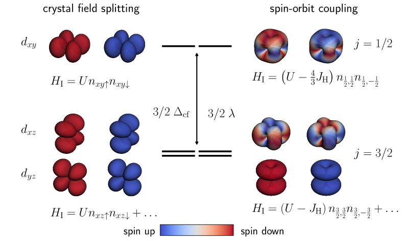
Figure 1: Energy levels of the considered models. For both SOC and tetragonal crystal-field splitting, the orbitally threefold degenerate $t_{2g}$ level splits into a twodfold degenerate and a onefold degenerate level. Each level has an additional spin degeneracy. In case of the crystal field, the $d_{xy}$ orbital is higher in energy, whereas it is the $j=1/2$ orbital in case of SOC. The respective orbitals are plotted left (crystal field) and right (SOC) of the energy levels. The color denotes the spin. The fact that the interaction matrix elements in the $j$ basis differ from the ones in the cubic $t_{2g}$ basis is also indicated in the figure.

The ground-state energies and the atomic charge gaps for a Kanamori Hamiltonian with spin-orbit coupling have been already analyzed in the supplementary material of Ref. [44]. Here, we briefly recapitulate certain limits and compare them to the case of a tetragonal crystal-field splitting. The SOC lowers the energy of the $j=3/2$ bands by $\lambda/2$ and increases the energy of the $j=1/2$ orbitals by $\lambda$. Therefore, the crystal-field splitting parameter $\Delta_{\textnormal{cf}}$ is chosen such that it increases the on-site energy of one orbital by $\Delta_{\textnormal{cf}}$ and that it lowers the energy of the other two by $\Delta_{\textnormal{cf}}/2$ in accordance with the effect of $\lambda$. Physically, this crystal field corresponds to a tetragonal tensile distortion in the $z$ direction. Both $\lambda$ and $\Delta_{\textnormal{cf}}$ are supposed to be positive; a negative sign would correspond to a particle-hole transformation. In Fig. 1 we illustrate the effects of the SOC and the tetragonal crystal field on the energy levels and also include a real-space representation of the respective orbitals. Although the SOC and the considered crystal field give an identical splitting of the single-electron energy levels, the corresponding orbitals and hence also the corresponding matrix elements are different, which has important consequences as discussed below.

Before discussing the issue of the interactions, let us briefly discuss the noninteracting case. Since both SOC and tetragonal crystal field lift the orbital degeneracy, they change the kinetic energy in the system. Without interactions where SOC and crystal field are equivalent, the kinetic energy can be readily calculated from the semicircular density of states, $E_{\textnormal{K}}=\int\epsilon\rho(\epsilon)f(\epsilon)d\epsilon$, with $f(\epsilon)$ the Fermi function at $T=0$. The SOC suppresses the noninteracting kinetic energy. In the large-$\lambda$ limit we find $E_{\textnormal{K}}(0)/E_{\textnormal{K}}(\lambda\to\infty)$ to be 1.13, 1.34, 1.96, and 1.73 for the cases $N=1$, $2$, $3$, and $5$, respectively (for $N=4$, the large-$\lambda$ limit corresponds to a band insulator with a vanishing kinetic energy). The reduction of kinetic energy due to the SOC was discussed in the case of the $N=3$ compound NaOsO3, where even a somewhat larger reduction of 2.3 was found in a realistic density-functional simulation [56].

We now turn to the atomic problem with interactions. It is instructive to rewrite the Kanamori Hamiltonian to the $j$ basis,

$$H_{\textnormal{I}}=\sum_{abcd}U_{abcd}c^{\dagger}_{a}c^{\dagger}_{b}c_{d}c_{c}=\sum_{\alpha\beta\gamma\delta}\tilde{U}_{\alpha\beta\gamma\delta}d^{\dagger}_{\alpha}d^{\dagger}_{\beta}d_{\delta}d_{\gamma}$$ (6)

with

$$\tilde{U}_{\alpha\beta\gamma\delta}=\sum_{abcd}U_{abcd}A^{*}_{\alpha a}A^{*}_{\beta b}A_{\gamma c}A_{\delta d},$$ (7)

where $A$ is the unitary transformation between the cubic $t_{2g}$ and the $j$ basis [57]. The Latin indices are combined indices of orbital and spin; the Greek indices are combined indices of $j$ and $m_{j}$. As the Kanamori Hamiltonian is invariant under this transformation for $J_{\textnormal{H}}=0$ [seen easily from Eq. (5)], the result of the crystal-field splitting and the SOC is identical in this case.

On the other hand, for a finite Hund’s coupling, the crystal field and SOC lead to different results. The transformed Hamiltonian in the $j$ basis differs from its form in the cubic basis (4). We can split it into a pure $j=1/2$ part, a pure $j=3/2$ part, and a part that mixes the $j=1/2$ and $j=3/2$ parts,

$$H_{\textnormal{I}}=H_{j=\frac{1}{2}}+H_{j=\frac{3}{2}}+H_{\textnormal{mix}}.$$ (8)

The first two terms read

$$H_{j=\frac{1}{2}}=\left(U-\frac{4}{3}J_{\textnormal{H}}\right){n_{\frac{1}{2},\frac{1}{2}}}{n_{\frac{1}{2},-\frac{1}{2}}},$$ (9)

$$\begin{split}H_{j=\frac{3}{2}}&=\left(U-J_{\textnormal{H}}\right)\left({n_{\frac{3}{2},\frac{3}{2}}}{n_{\frac{3}{2},-\frac{3}{2}}}+{n_{\frac{3}{2},\frac{1}{2}}}{n_{\frac{3}{2},-\frac{1}{2}}}\right)\\ &\quad+\left(U-\frac{7}{3}J_{\textnormal{H}}\right)\left({n_{\frac{3}{2},-\frac{3}{2}}}{n_{\frac{3}{2},-\frac{1}{2}}}+{n_{\frac{3}{2},\frac{3}{2}}}{n_{\frac{3}{2},\frac{1}{2}}}\right)\\ &\quad+\left(U-\frac{7}{3}J_{\textnormal{H}}\right)\left({n_{\frac{3}{2},-\frac{3}{2}}}{n_{\frac{3}{2},\frac{1}{2}}}+{n_{\frac{3}{2},\frac{3}{2}}}{n_{\frac{3}{2},-\frac{1}{2}}}\right)\\ &\quad+\frac{4}{3}J_{\textnormal{H}}\;d^{\dagger}_{\frac{3}{2},-\frac{3}{2}}d^{\dagger}_{\frac{3}{2},\frac{3}{2}}d_{\frac{3}{2},-\frac{1}{2}}d_{\frac{3}{2},\frac{1}{2}}\\ &\quad+\frac{4}{3}J_{\textnormal{H}}\;d^{\dagger}_{\frac{3}{2},-\frac{1}{2}}d^{\dagger}_{\frac{3}{2},\frac{1}{2}}d_{\frac{3}{2},-\frac{3}{2}}d_{\frac{3}{2},\frac{3}{2}},\end{split}$$ (10)

the density-density part of $H_{\textnormal{mix}}$ is

$$\begin{split}H_{\textnormal{mix, dd}}=&\left(U-\frac{5}{3}J_{\textnormal{H}}\right)\left({n_{\frac{1}{2},\frac{1}{2}}}{n_{\frac{3}{2},\frac{3}{2}}}+{n_{\frac{1}{2},-\frac{1}{2}}}{n_{\frac{3}{2},-\frac{3}{2}}}\right)\\ &+\left(U-2J_{\textnormal{H}}\right)\left({n_{\frac{1}{2},\frac{1}{2}}}{n_{\frac{3}{2},\frac{1}{2}}}+{n_{\frac{1}{2},-\frac{1}{2}}}{n_{\frac{3}{2},-\frac{1}{2}}}\right)\\ &+\left(U-\frac{7}{3}J_{\textnormal{H}}\right)\left({n_{\frac{1}{2},\frac{1}{2}}}{n_{\frac{3}{2},-\frac{1}{2}}}+{n_{\frac{1}{2},-\frac{1}{2}}}{n_{\frac{3}{2},\frac{1}{2}}}\right)\\ &+\left(U-\frac{8}{3}J_{\textnormal{H}}\right)\left({n_{\frac{1}{2},\frac{1}{2}}}{n_{\frac{3}{2},-\frac{3}{2}}}+{n_{\frac{1}{2},-\frac{1}{2}}}{n_{\frac{3}{2},\frac{3}{2}}}\right).\end{split}$$

The convention is that ${n_{\frac{1}{2},\frac{1}{2}}}$, for example, means $n_{j=\frac{1}{2},m_{j}=\frac{1}{2}}$. $H_{\textnormal{mix}}$ contains 30 more terms that are not shown here.

$H_{j=\frac{1}{2}}$ is a one-band Hubbard Hamiltonian with an effective interaction $U_{\textnormal{eff}}=U-4/3\,J_{\textnormal{H}}$. For the density-density part of $H_{j=\frac{3}{2}}$, one observes that the terms with the same $\left|m_{j}\right|$’s have prefactors $U-J_{\textnormal{H}}$, whereas terms with different $\left|m_{j}\right|$’s have prefactors $U-7/3J_{\textnormal{H}}$. If one uses $\left|m_{j}\right|$ as the orbital index and the sign of $m_{j}$ as the spin, the density-density part of this Hamiltonian is similar to the density-density part of a two-band Kanamori Hamiltonian, but with different prefactors. Importantly, there is only one kind of prefactor for interorbital interactions, namely $U-7/3J_{\textnormal{H}}$, instead of $U-2J_{\textnormal{H}}$ and $U-3J_{\textnormal{H}}$ in Eq. (4). This influences the electronic correlations, as we will see below in the case of $N=2$. Following this interpretation of the $m_{j}$’s, the last two terms are pair-hopping-like expressions with an effective strength of $4/3\,J_{\textnormal{H}}$. A detailed analysis of this Hamiltonian can be found in Appendix A.

It is useful to characterize the atomic Hamiltonian $H_{\textnormal{loc}}=H_{\textnormal{I}}+H_{\lambda}$ in terms of the atomic charge gap

$$\Delta_{\textnormal{at}}=E_{0}(N+1)+E_{0}(N-1)-2E_{0}(N),$$ (11)

where $E_{0}(N)$ is the ground state of a system with $N$ electrons [27]. According to the Mott-Hubbard criterion, the metal-insulator transition takes place when $\Delta_{\textnormal{at}}$ exceeds the kinetic energy. Hence, the proximity of interaction parameters to the associated critical value $U_{\textnormal{c}}$ can be used to anticipate the strength of electronic correlations.

We start with a discussion of the crystal-field splitting [58, 59, 60, 61]. For fillings $N=1$, $2$, and $5$, the ground state does not change with the crystal-field splitting. For $N=3$ and $N=4$, there is a level crossing with a transition from a high-spin to a low-spin state (e.g., from $\ket{\uparrow,\uparrow,\uparrow}$ to $\ket{\uparrow\downarrow,\uparrow,0}$), which is responsible for differences in the atomic charge gap for small and large $\Delta_{\textnormal{cf}}$. The respective values for the charge gap in the limits of small and large $\Delta_{\textnormal{cf}}$ are listed in Tables 1 and  2. Note that in the large $\Delta_{\textnormal{cf}}$ limit, the relevant Hamiltonian is a two-orbital one for fillings $N=1,2,$ and $3$, and a one-orbital one for $N=5$. For the Kanamori Hamiltonian with $\nu$ orbitals, the charge gap depends on the relative filling; at half filling it is $\Delta_{\textnormal{at}}=U+(\nu-1)J_{\textnormal{H}}$, otherwise $U-3J_{\textnormal{H}}$. The filling $N=4$ is special as an electron can only be added by paying additionally crystal-field splitting energy.

We now turn to the discussion of SOC. Note that the limits $\lambda\ll J_{\textnormal{H}}$ and $\lambda\gg J_{\textnormal{H}}$ correspond to the $LS$ and $jj$ coupling scheme, respectively. A look at Tables 1 and 2 reveals that practically all entries are different from the corresponding crystal-field ones. The values for a large SOC can be obtained from the Hamiltonian expressed in the $j$ basis discussed above. For $N=5$, where the effective model is a single-orbital model, the interaction parameter is $U-\frac{4}{3}J_{\textnormal{H}}$, as seen from Eq. (9), in contrast to the crystal field result, where one obtains simply $U$, instead. In the case of $N=2$, it is interesting to note that the dependence of the charge gap on $J_{\textnormal{H}}$ is different in sign for the SOC and the crystal field. This follows from Eq. (10), which does not favor the alignment of the angular momenta $j_{z}$ of the respective orbitals (see also Appendix A). This opposite behavior is also reflected in the full DMFT solution, as we discuss below. We will see that for $N=2$, there are parameter regimes, where the correlation strength increases with crystal-field splitting, but it decreases with SOC.

Table 1: Comparison of the atomic charge gap $\Delta_{\textnormal{at}}$ obtained from a spin-orbit coupling $\lambda$ or a tetragonal crystal-field splitting $\Delta_{\textnormal{cf}}$ in the limit $\lambda,\Delta_{\textnormal{cf}}\ll J_{\textnormal{H}}$.

$N$	SOC	crystal field
1	$\,\,\,U-3J_{\textnormal{H}}+1/2\,\lambda\,\,\,$	$U-3J_{\textnormal{H}}$
2	$U-3J_{\textnormal{H}}+1/2\,\lambda$	$\,\,\,U-3J_{\textnormal{H}}+3/2\,\Delta_{\textnormal{cf}}\,\,\,$
3	$U+2J_{\textnormal{H}}-3/2\,\lambda$	$U+2J_{\textnormal{H}}-3/2\,\Delta_{\textnormal{cf}}$
4	$U-3J_{\textnormal{H}}+\lambda$	$U-3J_{\textnormal{H}}$
5	$U-3J_{\textnormal{H}}+\lambda$	$U-3J_{\textnormal{H}}+3/2\,\Delta_{\textnormal{cf}}$

Table 2: Comparison of the atomic charge gap $\Delta_{\textnormal{at}}$ obtained from a spin-orbit coupling $\lambda$ or a tetragonal crystal-field splitting $\Delta_{\textnormal{cf}}$ in the limit $\lambda,\Delta_{\textnormal{cf}}\gg J_{\textnormal{H}}$.

$N$	SOC	crystal field
1	$U-7/3\,J_{\textnormal{H}}$	$U-3J_{\textnormal{H}}$
2	$U-J_{\textnormal{H}}$	$U+J_{\textnormal{H}}$
3	$U-7/3\,J_{\textnormal{H}}$	$U-3J_{\textnormal{H}}$
4	$\,\,\,U-3J_{\textnormal{H}}+3/2\,\lambda\,\,\,$	$\,\,\,U-5J_{\textnormal{H}}+3/2\,\Delta_{\textnormal{cf}}\,\,\,$
5	$U-4/3\,J_{\textnormal{H}}$	$U$

IV DMFT results

We now turn to the DMFT results. We focus on the interplay between the SOC and electronic correlations, which we follow by calculating the Matsubara self-energies. Due to the symmetry, the Green’s functions and the self-energies are diagonal in the $j$ basis with two independent components $\Sigma_{1/2}$ and $\Sigma_{3/2}$.

Figure 2 displays the calculated self-energies for the $N=1$ case. One can see that due to the SOC $|\mathrm{Im}\Sigma_{3/2}|$ is larger and its slope at low energies that determines the quasiparticle residue

$$Z_{\nu}=\lim\limits_{i\omega_{n}\rightarrow 0}\left[1-\frac{\partial\textnormal{Im}\Sigma_{\nu}(i\omega_{n})}{\partial i\omega_{n}}\right]^{-1}$$ (12)

is larger. The origin of that is discussed below, where we investigate the evolution of $Z_{\nu}$ with $\lambda$ for all integer occupancies, but let us first discuss the other part of the interplay, namely the influence of the electronic correlations on the SOC.

IV.1 Influence of electronic correlations on the SOC; effective SOC

For this purpose it is convenient to introduce the average self-energy

$$\Sigma_{\textnormal{a}}=\frac{2}{3}\Sigma_{\frac{3}{2}}+\frac{1}{3}\Sigma_{\frac{1}{2}}$$ (13)

and the difference

$$\Sigma_{\textnormal{d}}=\Sigma_{\frac{1}{2}}-\Sigma_{\frac{3}{2}}.$$ (14)

In terms of $\Sigma_{\textnormal{a,d}}$ the self-energy matrix can be written in the form

$$\Sigma=\Sigma_{\textnormal{a}}\mathbb{1}+\frac{2}{3}\Sigma_{\textnormal{d}}\mathbf{l}_{t_{2g}}\cdot\mathbf{s},$$ (15)

which holds in any basis (see Appendix B). This form is also convenient as one can directly see that $\Sigma_{\textnormal{d}}$ determines the influence of electronic correlations on the physics of SOC.

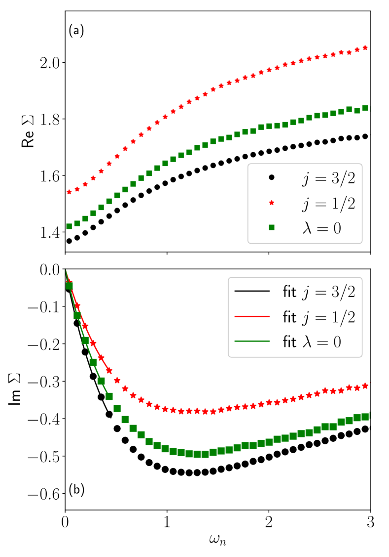
Figure 2: Real (a) and imaginary (b) part of the self-energy for the parameters $N=1$, $\lambda=0.1$, $U=3$, and $J_{\textnormal{H}}=0.1\,U$. The green squares display the results without SOC for comparison. The lines show a polynomial fit of degree four through the first six Matsubara frequencies.

In particular, because the Green’s function is

$$G(k,i\omega_{n})=\left[i\omega_{n}+\mu-H_{0}(k)-\Sigma(i\omega_{n})\right]^{-1}$$ (16)

with $H_{0}(k)$ the noninteracting Hamiltonian that includes the SOC, the real part of the self-energy can be used to define the effective spin-orbit-coupling constant

$$\lambda_{\textnormal{eff}}=\lambda+\frac{2}{3}\,\mathrm{Re}\Sigma_{\textnormal{d}}(i\omega_{n}\to 0).$$ (17)

For all cases we looked at (some data is shown in Appendix B), we find that the real part of $\Sigma_{\textnormal{d}}(i\omega_{n})$ is positive for all $\omega_{n}$ (as long as the system is metallic) and its effect hence adds up to the bare SOC Hamiltonian so that $\lambda_{\textnormal{eff}}>\lambda$, as found also in realistic studies [40, 21, 22]. Notice that there is also a further renormalization of the overall bandstructure due to the frequency dependence of the self-energy [41, 22]. The effects on the quasiparticle dispersions, for instance on the liftings of the quasiparticle degeneracies, can be phrased in terms of the quasiparticle SOC constant $\lambda^{*}=Z\lambda_{\textnormal{eff}}$ [22] with quasiparticle renormalization $Z<1$, hence $\lambda^{*}$ can be smaller or larger than the bare $\lambda$. However, relative to the other features of the quasiparticle dispersions that are obviously renormalized by $Z$, too, the SOC splittings are enhanced due to the effect of $\Sigma_{\textnormal{d}}$.

IV.2 Influence of SOC on electronic correlations: One and five electrons

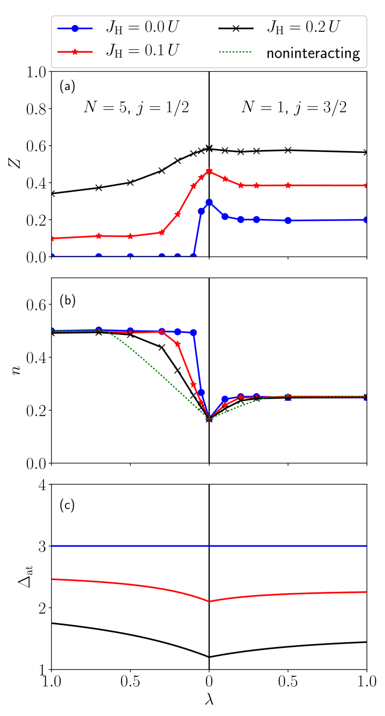
Figure 3: Influence of the spin-orbit coupling for a filling of $N=1$ (right column) and $N=5$ (left column) for $U=3$. (a) Quasiparticle weight $Z$ of the $j=3/2$ orbitals (for $N=1$) and of the $j=1/2$ orbitals (for $N=5$). (b) Electron density $n$ of the $j=3/2$ orbitals ($N=1$) and hole density of the $j=1/2$ orbitals ($N=5$) to allow for a better comparability. The green dotted line displays the respective noninteracting results. (c) Atomic charge gap $\Delta_{\textnormal{at}}$.

In the remainder of the paper we investigate how the SOC influences the electronic correlations, which is followed by calculating the $j$-orbital occupations and the quasiparticle residues $Z_{\nu}$. These are calculated by fitting six lowest frequency points of Matsubara self-energies to a fourth order polynomial, as shown in Fig. 2(b).

Without SOC, one electron and one hole (five electrons) in the system are equivalent due to the particle-hole symmetry, but the SOC breaks this symmetry. For large $\lambda$, only the $j=3/2$ ($j=1/2$) orbitals are partially occupied for $N=1$ ($N=5$). Hence, these are more interesting regarding electronic correlations. In Figs. 3(a) and 3(b), we show how the quasiparticle weights and the fillings of these orbitals change when the SOC is increased. The corresponding atomic charge gap is also plotted, Fig. 3(c).

The change in orbital polarization influences the correlation strength. This is best seen for $J_{\textnormal{H}}=0$, since then the effective repulsion is simply $U$, independent of the SOC. The quasiparticle weight of the relevant orbitals is reduced by the SOC as the polarization increases, which is shown in Fig. 3(b) for $U=3$ (circles). The reduction is weak for $N=1$ but strong for $N=5$, which is due to the lower kinetic energy of one hole in one $j=1/2$ orbital compared to the energy of one electron in two $j=3/2$ orbitals. In the case of $U=3$ and $J_{\textnormal{H}}=0$, even a metal-insulator transition takes place.

The Hund’s coupling reduces the correlation strength (stars, crosses). This happens for two reasons: $J_{\textnormal{H}}$ reduces the polarization, and it decreases the atomic charge gap. The latter is expected for $N=1$, where the effective number of orbitals reduces with increasing $\lambda$ from three to two. In this case, a finite exchange interaction $J_{\textnormal{H}}$ leads to a reduction of the repulsion between electrons in different orbitals.

Interestingly, $J_{\textnormal{H}}$ also decreases the strength of correlations for $N=5$ in the limit of large $\lambda$, although the effective number of orbitals is one and interorbital effects are thus suppressed. However, the transformation from the cubic Kanamori Hamiltonian to its $j$ basis equivalent mixes inter- and intraorbital interactions, so that the effective $j=1/2$ interaction strength is $U-4/3\,J_{\textnormal{H}}$, as explained in Sec. III. In contrast, in the case of a large tetragonal crystal-field splitting, the atomic charge gap is indeed simply given by $U$ for $N=5$.

It is also interesting to compare the dependence of the respective orbital occupation $n$ with the noninteracting result [green dotted line in Fig. 3(b)]. One can see that the correlations increase the orbital polarization $n_{3/2}-n_{1/2}$, in line of what one would expect from the enhancement of the SOC physics by electronic correlations discussed above. As shown below, we find similar behavior also for other fillings, but not for $N=3$ when the Hund’s coupling is large.

IV.3 Half filling

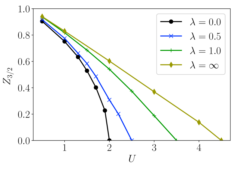
Figure 4: Quasiparticle weight $Z_{3/2}$ of the $j=3/2$ orbital as a function of $U$ for $J_{\textnormal{H}}=0.1\,U$ and a total filling of $N=3$.

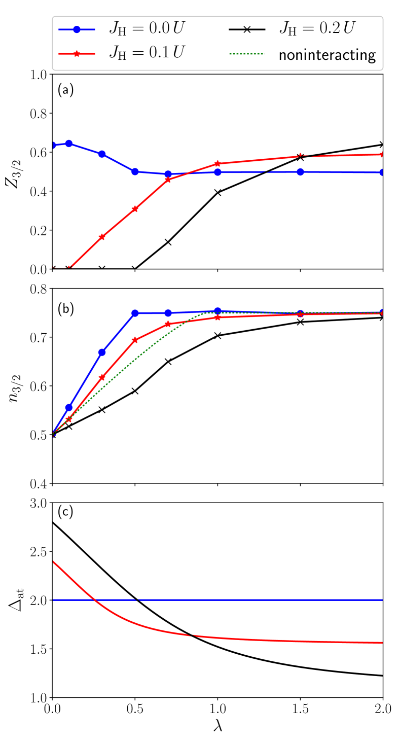
Figure 5: Quasiparticle weight $Z_{3/2}$ (a) and filling $n_{3/2}$ (b) of the electrons in the $j=3/2$ orbitals as functions of $\lambda$ for $U=2$. The green dotted line displays the respective noninteracting results. (c) Atomic charge gap $\Delta_{\textnormal{at}}$.

In Fig. 4 we display the quasiparticle weight of the $j=3/2$ orbitals (again, the $j=1/2$ are emptied out with SOC and are therefore not discussed here) at $N=3$ for several $\lambda$. One can see that $\lambda$ strongly increases $U_{\textnormal{c}}$ and changes the behavior drastically. To understand why this occurs, first recall that at $\lambda=0$, Hund’s coupling strongly reduces the kinetic energy since it enforces the high-spin ground state [25]. Hence, the Hund’s coupling leads to a drastic reduction of the critical interaction strength [26]. This causes a steep descent of $Z$ as a function of $U$ when the critical $U$ is approached (see Fig. 4 for $\lambda=0$ and $J_{\textnormal{H}}=0.1\,U$).

As $\lambda$ is large, this physics does not apply any more. The filling of the $j=3/2$ orbitals increases to three electrons in two orbitals. Since the Hamiltonian of the $j=3/2$ orbitals alone is particle-hole symmetric, this large $\lambda$ limit shows identical physics to the large $\lambda$ limit in the case of $N=1$. As described above in Sec. IV.2, this $\lambda\rightarrow\infty$ system is characterized by an increase of $Z$ with increasing $J_{\textnormal{H}}$. This is opposite to the half-filled $N=3$ case at $\lambda=0$, where $Z$ decreases with $J_{\textnormal{H}}$.

In Figs. 5(a)-5(c) we show how the quasiparticle weight, the orbital polarization, and the atomic charge gap vary with $\lambda$, respectively. We find that $Z$ increases for physically relevant Hund’s couplings (e.g., $J_{\textnormal{H}}=0.1\,U$, $J_{\textnormal{H}}=0.2\,U$). Furthermore, the qualitative difference between the small and the large $\lambda$ limits discussed above results in crossings of the $Z(\lambda)$ curves for different Hund’s couplings [see Fig. 5(a)]. These crossings are already expected from the atomic charge gap, which is $U+2J_{\textnormal{H}}$ for $\lambda=0$ and drops to $U-7/3J_{\textnormal{H}}$ for $\lambda\rightarrow\infty$, as shown in Tables 1 and 2 as well as in Fig. 5(c).

The results in Fig. 5 show that SOC can strongly modify the correlation strength. One needs to notice, though, that it takes a quite large $\lambda$ for these changes to occur; for instance, full polarization is reached at $\lambda\approx 1$, whereas it occurs at $\lambda\approx 0.3$ in the case of $N=1$ and $U=3$ (compare Fig. 5 with Fig. 3). In this respect we notice also that in contrast to the $N=1$ case, the electronic correlations increase the orbital polarization at $N=3$ as compared to the noninteracting result only for small values of $J_{\textnormal{H}}$.

IV.4 Two electrons

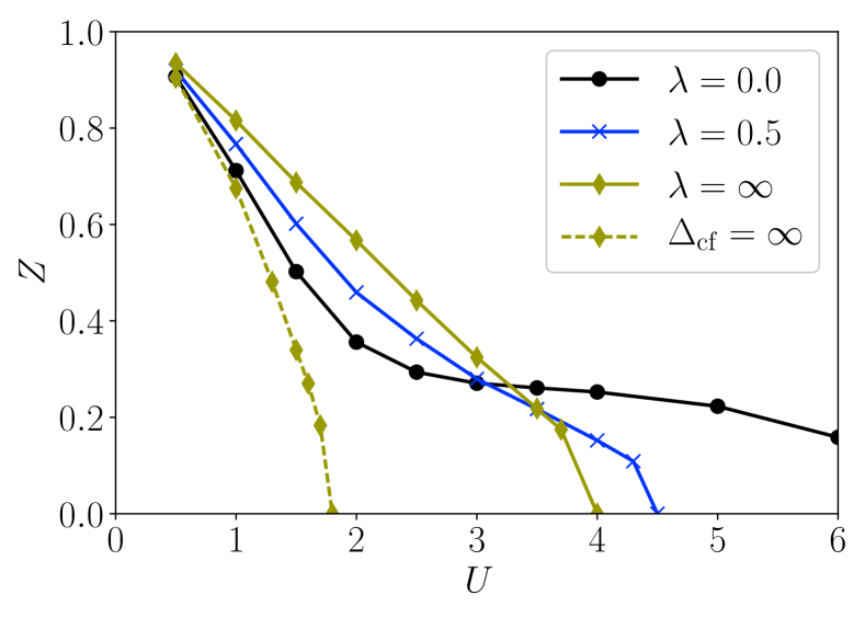
Figure 6: Quasiparticle weight $Z$ of the $j=3/2$ orbital as a function of $U$ for $J_{\textnormal{H}}=0.2\,U$ and $N=2$. The dashed line shows the corresponding $Z$ of the $d_{xz}$ orbital in the case of an infinite tetragonal crystal-field splitting.

We now discuss the interesting case of two electrons. In the absence of SOC, this is the case of a Hund’s metal. Figure 6 shows the dependence of $Z$ on $U$ for several values of $\lambda$ and $J_{\textnormal{H}}/U=0.2$. The data at small $\lambda$ exhibit a tail with small $Z$, which is characteristic for the Hund’s metal regime. The SOC has a drastic effect here; increasing $\lambda$ suppresses the Hund’s metal behavior and leads to a featureless, almost linear, approach of $Z$ towards 0 with increasing $U$. Interestingly, the influence of $\lambda$ on $Z$ is opposite at small $U$ where increasing $\lambda$ increases $Z$, thus making the system less correlated, and at a high $U$, where $Z$ diminishes with $\lambda$ and hence correlations become stronger.

The latter behavior is easy to understand. A strong SOC reduces the number of relevant orbitals from three to two, and leads to the increase of the atomic charge gap from $U-3J_{\textnormal{H}}$ to $U-J_{\textnormal{H}}$ [see Fig. 8(c) and Sec. III]. Both the reduction of the kinetic energy due to the reduced degeneracy and the increase of the atomic charge gap with $\lambda$ contribute to a smaller critical $U$, which is indeed seen on the plot. We want to note here that the reduction of the critical $U$ is even stronger for the crystal-field case (shown as a dashed line in Fig. 6), since there the corresponding atomic gap is larger ($U+J_{\textnormal{H}}$, see Sec. III).

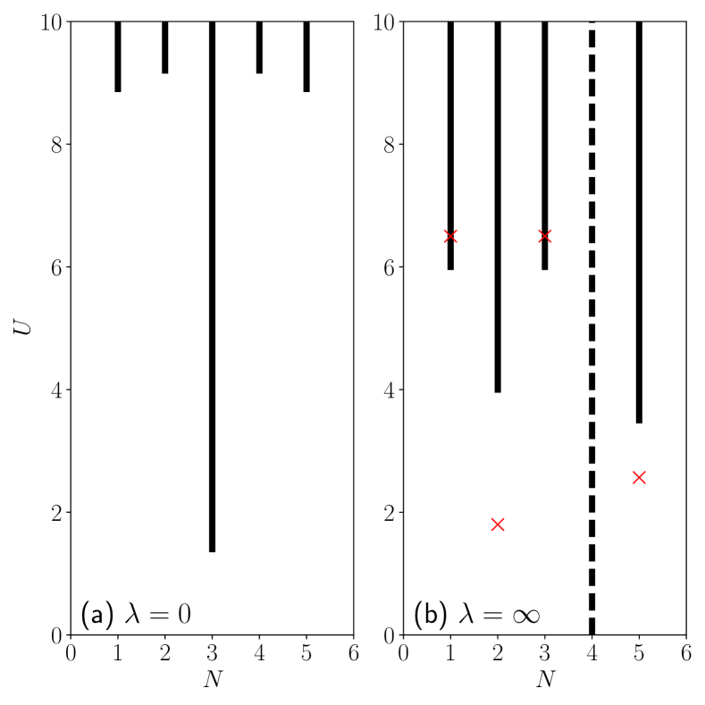
Figure 7: The Mott insulator occurs for values of $U$ indicated by bars for a Hund’s coupling of $J_{\textnormal{H}}=0.2\,U$. The left picture (a) shows the case without SOC, the right (b) with an infinite SOC. Note that in the latter case no Mott insulator occurs for $N=4$ since this case is a band insulator. The critical values for $\lambda=0$ are taken from Ref. 26. The red crosses indicate the critical $U$ in the case where a tetragonal crystal field is applied instead of the SOC.

We turn now to the small-$U$ regime where the SOC reduces the electronic correlations. One can rationalize this from a scenario that pictures Hund’s metals as doped Mott insulators at half filling [33, 34, 35, 36]. Figure 7 presents the values of $U$ where a Mott insulator occurs. Let us first discuss the case without SOC, i.e., the left panel of Fig. 7. In this picture of doped Mott insulators, the correlations for small interactions at $N=2$ are due to proximity to a half-filled insulating state. For interaction parameters $U$ and $J_{\textnormal{H}}$ that lead to a Mott insulator at half filling, doping with holes leads to a metallic state with low quasiparticle weight. This low-$Z$ region persists to doping concentrations of more than one hole per atom, as can be seen from Fig. 2 in Ref. [26]. As a result, for an interaction $U$ in between the critical values for two and three electrons $U_{\textnormal{c}}(N=3)<U<U_{\textnormal{c}}(N=2)$, the quasiparticle weight is small, but not zero. As one increases now $\lambda$, the critical $U$ at $N=3$ increases strongly, and the insulating state appears only for large values of $U$, see the right panel of Fig. 7. Consequently, the $N=2$ state cannot be viewed as a doped $N=3$ Mott insulator any more. In fact, for a large SOC, the critical interaction strength $U_{\textnormal{c}}$ for a Hund’s coupling of $J_{\textnormal{H}}/U=0.2$ is lowest for $N=2$, as displayed in Fig. 7. As a consequence, the Hund’s tail disappears (this was earlier noted also in a rotationally-invariant slave boson study of a five orbital problem [45]), as highlighted in Fig. 6, and the quasiparticle weight increases with SOC in the case of a small $U$ and large Hund’s couplings [see Fig. 8(a)]. In passing we note that the DMFT self-consistency is essential to account for the increase of $Z$ in the small $U$ regime. Calculations for an impurity model found a suppression of the Kondo temperature (and hence a suppression of $Z$) with increased $\lambda$ [43], which is different from what we find in the DMFT results here.

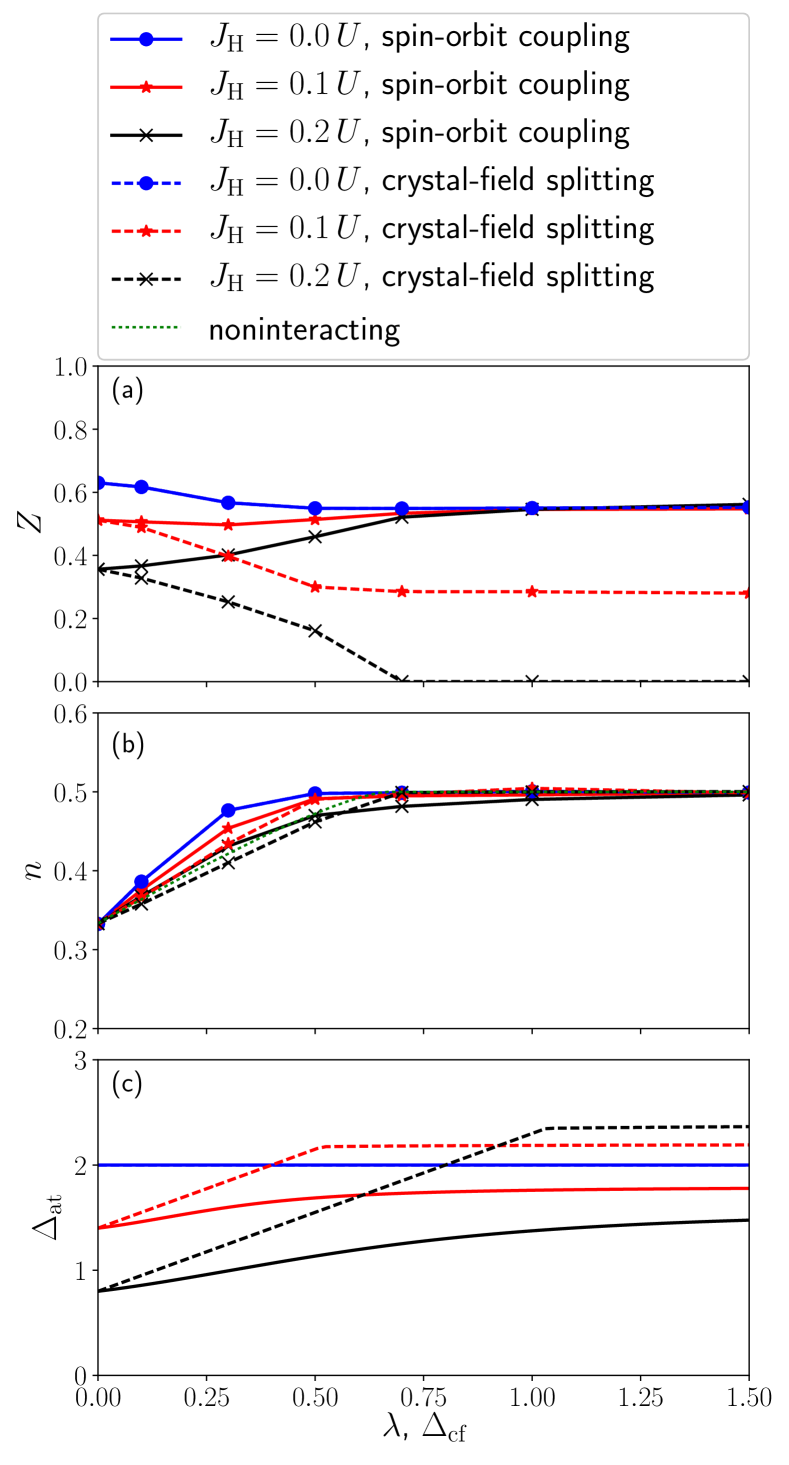
Figure 8: Quasiparticle weight of the electrons (a), filling (b), and the atomic charge gap (c) for $N=2$ and $U=2$. Solid lines correspond to the SOC case, and $j=3/2$ quantities are plotted as functions of $\lambda$. Dashed lines are the results for a crystal-field splitting, where we plot $d_{xz/yz}$ quantities as functions of $\Delta_{\textnormal{cf}}$.

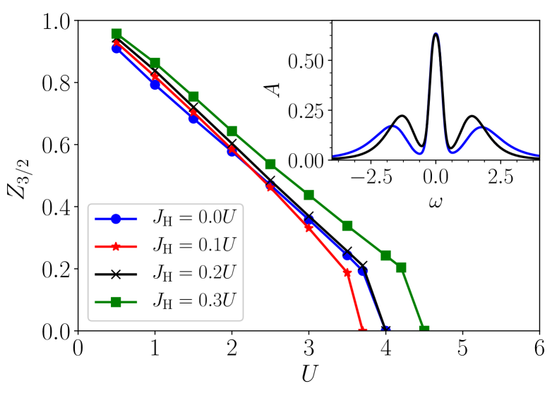
Figure 9: Quasiparticle weight $Z_{3/2}$ of the $j=3/2$ orbital as a function of $U$ for $\lambda\rightarrow\infty$ and a total filling of $N=2$. The inset shows the respective impurity spectral functions for $U=3$ and $J_{\textnormal{H}}=0$ (blue) and $J_{\textnormal{H}}=0.2\,U$ (black). As the Hund’s coupling $J_{\textnormal{H}}$ increases, the quasiparticle weight (= area of the quasiparticle peak) stays the same, whereas the position of the Hubbard bands changes due to different charge gaps. To obtain the spectral functions, imaginary-time data has been analytically continued using a maximum entropy method [62] with an alternative evidence approximation [63] and the preblur formalism [64].

Figure 8(b) shows the orbital occupancy as a function of $\lambda$. Like in $N=1$, $N=5$, and, for small enough $J_{\textnormal{H}}$, also $N=3$, from a comparison with the noninteracting result one finds that the SOC usually leads to a larger orbital polarization when the interactions are present. Looking at the data more precisely, this ceases to hold in the large-$\lambda$ regime. We actually find this at other fillings, too. At values of $\lambda$ where the noninteracting result is already fully polarized, the electronic correlations reintroduce some charge in the empty/fully polarized orbital.

In Fig. 8, we also compare the influence of the SOC to that of a tetragonal crystal field. One sees that the crystal field always increases the correlation strength. To understand this it is convenient to recall that the atomic gaps are different, and as a result, also the critical $U$’s are different. For an infinite crystal field, they are marked with crosses in Fig. 7(b). In particular, the critical interaction at $N=2$ in the case of an infinite crystal field is only slightly larger than the critical interaction at $N=3$ without any splitting. Therefore, Hund’s metals with interactions in the range $U_{\textnormal{c}}(N=3)<U<U_{\textnormal{c}}(N=2)$, becomes insulating, as the interaction driven Mott transition at $N=2$ is pushed to such small values of $U_{\textnormal{c}}$ by the large $\Delta_{\textnormal{cf}}$. Another difference is the ground state degeneracy, which is three for the $S=1$ ground state of the two-orbital Kanamori and five in the case of the $J=2$ ground state of $H_{j=3/2}$, see Appendix A, which also points to weaker correlations in the SOC case.

Another interesting observation from Fig. 8(a) is that the quasiparticle weight is almost independent of Hund’s coupling in the limit of large $\lambda$ for $U=2$. In Fig. 9, we show that the weak dependence on $J_{\textnormal{H}}$ is also apparent for other values of $U$, and only becomes significant when the Hund’s coupling is exceeding $J_{\textnormal{H}}>0.2\,U$. However, since the atomic gap does depend on $J_{\textnormal{H}}$, the position of the Hubbard bands are different, even though $Z$ is the same, as shown in the inset of Fig. 9.

IV.5 Four electrons

The filling of four electrons is special because strong SOC leads to a band insulator with fully occupied $j=3/2$ orbitals and empty $j=1/2$ orbitals, with no renormalization ($Z=1$) for both orbitals in the large $\lambda$ regime.

Figure 10(a) shows the quasiparticle renormalization of both orbitals in the metallic phase as a function of $\lambda$. One can see that $Z_{3/2}$ is hardly affected, and $Z_{1/2}$ increases only slightly for the given parameters $U=2$ and $J_{\textnormal{H}}=0.2\,U$, indicating that the orbital polarization affects only weakly the correlation strength, unless in close vicinity to the metal-insulator transition.

A comparison to the crystal-field results shows two major differences: First, the orbital polarization, displayed in Fig. 10(b), is smaller in the case of the crystal field, as compared to the SOC case, and a larger value of crystal-field splitting is needed to reach a band insulator. The reason for this is a larger atomic gap in the SOC case [see Fig. 10(c) and Tables 1 and 2]. Second, the quasiparticle renormalization of the less occupied (in the case of crystal field $d_{xy}$) orbital is lowest when its filling is around 1/2. This enhancement of correlation effects at half filling is absent for the $j=1/2$ orbital.

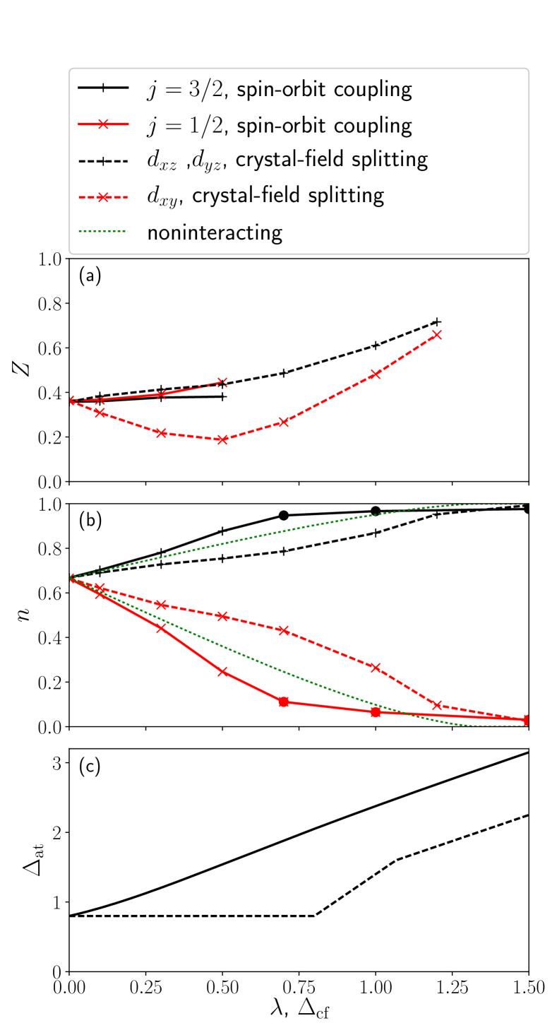
Figure 10: Quasiparticle renormalization (a), filling (b), and atomic charge gap (c) of the orbitals as functions of spin-orbit coupling (full lines) and crystal-field splitting (dashed lines) for $N=4$, $U=2$, $J_{\textnormal{H}}=0.2\,U$. Full dots indicate insulating phases. In the case of SOC, all calculations with $\lambda\geq 0.7$ are insulating, whereas in the case of a crystalfield only the last point shown ($\Delta_{\textnormal{cf}}=1.5$) is insulating. The green dotted lines shows the orbital fillings in the noninteracting case. Then, crystal field and SOC are equivalent.

IV.6 Discussion

It is interesting to discuss our results in the context of real materials and to consider which parameter regimes are realized (see also Refs. 19, 44). One can first recall the atomic values $\zeta$ for the SOC that roughly increase with the fourth power of the atomic number. It takes small values in 3$d$ (Mn: $0.04\text{\,}\mathrm{eV}$, Co: $0.07\text{\,}\mathrm{eV}$), intermediate values in 4$d$ (Ru: $0.13\text{\,}\mathrm{eV}$, Rh: $0.16\text{\,}\mathrm{eV}$), and reaches considerable strength in 5$d$ (Os: $0.42\text{\,}\mathrm{eV}$, Ir: $0.48\text{\,}\mathrm{eV}$) atoms [65]. These atomic values are representative also for the values of SOC $\lambda$ found in corresponding oxides. Regarding interaction parameters, one can roughly take that $J_{\textnormal{H}}/U=0.1$ and values of $U$ that diminish from $4\text{\,}\mathrm{eV}$(in 3$d$), $3\text{\,}\mathrm{eV}$(4$d$), $2\text{\,}\mathrm{eV}$(5$d$). Finally, the bandwidth will vary from case to case, since it depends the most on structural details among all the microscopic parameters. As a rule of thumb, however, it increases with the principle quantum number, giving values of half bandwidth from $D$=$1\text{\,}\mathrm{eV}$(3$d$), $1.5\text{\,}\mathrm{eV}$(4$d$), $2\text{\,}\mathrm{eV}$(5$d$). These all are of course only rough estimates, meant to indicate trends.

The clear-cut case with strong influence of SOC are 5$d$ oxides at $N=5$. In iridates, $\lambda/D$ ranges from 0.26 in Sr2IrO4 up to 2.0 in Na2IrO3 due to the small bandwidth in this compound [44]. Inspecting now Fig. 3, one sees that the SOC leads to a strong orbital polarization and strongly affects the correlations at those values of $\lambda/D$. Actually, the sensitivity to SOC at $N=5$ is so strong that one can expect significant impact also in $4d^{5}$ compounds, like rhodates, too, although $\lambda$ is by a factor of three smaller there. Indeed, the enhancement of correlations has been observed in a material-realistic DMFT study of Sr2RhO4 [18, 19]. Rather small SOC leads also to a large polarization in the particle-hole transformed counterpart $N=1$ (with potentially important consequences for the magnetic ordering [66]), but the increase of the quasiparticle renormalization is weak, see Fig. 3(a).

Opposite to the $N=1$ and $N=5$ cases, the SOC at $N=3$ makes the electronic correlations weaker. Also in contrast to the former two cases, the effect of SOC on polarization and quasiparticle renormalization becomes pronounced only at larger values of $\lambda$. From Fig. 5(b) we can infer that for full polarization $\lambda/D>0.5$ is necessary. Large values of $\lambda/D$ can be obtained in double perovskites based on $5d$ elements. In Sr2ScOsO6, for instance, quite a substantial reduction of correlations occurs with SOC [67]. In case of the single perovskite NaOsO3, the SOC modifies the band structure [68] too, which leads to an important suppression of kinetic energy [56], as discussed also in Sec. III. In the case of $4d$ elements, typically $\lambda/D<0.2$; therefore we expect only small effects of the SOC on the correlation strength in these materials.

For the filling $N=2$, we show in Fig. 6(a) a systematic suppression of the Janus-faced behavior with SOC, making the Hund’s tail disappear. This effect is already sizable for $\lambda/D\approx 0.5$ and should, hence, be present in many $5d$ systems. Indeed, it has been seen in calculations for the $5d^{2}$ compound Sr2MgOsO6 [67]. For a smaller SOC of $\lambda/D\approx 0.1$, which is a good estimate for many $4d$ materials, we do not find a substantial change of $Z$ [see, for example, Fig. 8(a)]. Therefore, we think the SOC only weakly affects the correlation strength in materials with $4d^{2}$ configuration, such as Sr2MoO4 [69, 70, 71].

For $N=4$, our model calculations predict that the SOC affects the correlation strength only a little, provided it is small enough such that the system remains in the metallic phase. If it exceeds a certain magnitude, though, a metal-insulator transition occurs. The critical $\lambda$ decreases with increasing $U$. Examples for this behavior are on one hand Sr2RuO4 ($\lambda$ = $0.10\text{\,}\mathrm{eV}$), where the quasiparticle renormalization hardly changes as the SOC is turned on [22], and, on the other hand, NaIrO3 ($\lambda$ = $0.33\text{\,}\mathrm{eV}$), where the interplay of SOC and $U$ leads to an insulating state [72].

V Conclusion

In this paper we investigated the influence of the SOC on the quasiparticle renormalization $Z$ in a three-orbital model on a Bethe lattice within DMFT. Depending on the filling of the orbitals (and for $N=2$ also the interaction strength), the SOC can decrease or increase the strength of correlations. The behavior can be understood in terms of the SOC-induced changes of the effective degeneracy, the fillings of the relevant orbitals, and the interaction matrix elements in the low-energy subspace.

The spin-orbital polarization leads to an increase of the correlation strength for $N=1$ and $5$, with particularly strong effect for $N=5$, where a half-filled single-band problem is realized, relevant for iridate compounds. For the nominally half-filled case $N=3$, the opposite trend is observed. Here, turning on SOC makes the system less correlated, and the critical interaction strength $U_{\textnormal{c}}$ for a Mott transition is increased. For the $N=2$ Hund’s metallic phase, the influence of SOC is more involved. We find that there are two regimes as a function of $U$ with opposite effect of SOC. For small $U$, the inclusion of SOC increases $Z$, whereas for large $U$ it decreases $Z$, and in turn also the critical interaction $U_{\textnormal{c}}$ decreases. As a result, the so-called Hund’s tail with small quasiparticle renormalization for a large region of interaction values, disappears.

We also considered the effects of the electronic correlations on SOC and found that in the cases where the system remains metallic, correlations always enhance the effective SOC.

Appendix A Atomic Hamiltonian in the limit of small and large spin-orbit couplings

The full local Hamiltonian reads [see also Eq. (5)]

$$\begin{split}H_{\textnormal{loc}}&=H_{\textnormal{I}}+H_{\lambda}+H_{\epsilon}\\ &=(U-3J_{\textnormal{H}})\frac{N(N-1)}{2}+\left(\frac{5}{2}J_{\textnormal{H}}+\epsilon\right)N\\ &\quad-2J_{\textnormal{H}}\mathbf{S}^{2}-\frac{J_{\textnormal{H}}}{2}\mathbf{L}^{2}+\lambda\,\mathbf{l}_{t_{2g}}\cdot\mathbf{s},\end{split}$$ (18)

with an SOC $\lambda$ and an on-site energy $\epsilon$. Note that this Hamiltonian contains both two-particle terms like $N^{2}$, $\mathbf{L}^{2}$, and $\mathbf{S}^{2}$, as well as one-particle terms like $N$ and $\mathbf{l}_{t_{2g}}\cdot\mathbf{s}$. For $\lambda=0$, the total spin $S$ and the total orbital angular momentum $L$ are good quantum numbers and determine together with the total number of electrons $N$ the eigenenergies. As $\lambda$ is finite, the energy levels split according to their total angular momentum $J$. For example, the nine-fold degenerate $S=1$, $L=1$ ground state in the $N=2$ sector splits into a $J=2$, a $J=1$, and a $J=0$ sector. The respective degeneracies are $2J+1$. The total angular momentum $J$ is for all values of $\lambda$ a good quantum number, in contrast to the total spin $S$ and the total orbital angular momentum $L$.

For a small SOC ($\lambda\ll J_{\textnormal{H}}$), one can use first-order perturbation theory in order to calculate the level splitting due to the SOC. In this approximation, the spin-orbit term is approximated by $C\lambda\,\mathbf{L}\cdot\mathbf{S}$. The constant $C$ depends on the number of electrons and is $C=1,1/2$ for one and two electrons, and $C=-1,-1/2$ for one and two holes. For three electrons, $L=0$, and the first-order perturbation theory gives no energy correction. Since the total angular momentum is approximated by $\mathbf{J}=\mathbf{L}+\mathbf{S}$, this regime is known as $LS$ coupling regime.

In the limit of large SOC ($\lambda\gg J_{\textnormal{H}}$), the spin-orbit term is the dominant term that is solved exactly, whereas $\mathbf{S}^{2}$ and $\mathbf{L}^{2}$ may be treated perturbatively. The many-body eigenstates of the unperturbed system are then the Slater determinants of $j=1/2$ and $j=3/2$ one-electron states. Following Eq. (2), the matrix elements of $\lambda\,\mathbf{l}_{t_{2g}}\cdot\mathbf{s}$ depend in this unperturbed eigenbasis only on the number of electrons in the $j=3/2$ and the $j=1/2$ orbitals. The total angular momentum is $\mathbf{J}=\sum_{i}\mathbf{j}_{i}$, therefore, this regime is the $jj$ coupling regime. For fillings $N\leq 4$, only the $j=3/2$ orbitals are occupied in the ground state. The spin-orbit term is then proportional to the particle number $N$ and can be absorbed in the one-electron energy $\epsilon$.

Calculating the matrix elements of $\mathbf{S}^{2}$ and $\mathbf{L}^{2}$ for Slater determinants with different $N$ and $J$ using Clebsch-Gordan coefficients, one can find the eigenenergies of the Hamiltonian in the $jj$ coupling regime. This approach is equivalent to looking for the eigenvalues of $H_{j=\frac{3}{2}}$ presented in Eq. (10) in the main text, where all contributions of the $j=1/2$ orbitals are neglected. The eigenenergies of $H_{j=\frac{3}{2}}$, including an on-site energy $\epsilon$, are shown in Table 3.

Table 3: Eigenenergies of the Hamiltonian $H_{j=\frac{3}{2}}$ of the $j=3/2$ orbitals, Eq. (10).

$N$	$J$	$E_{j=3/2}$
0	0	0
1	3/2	$\epsilon$
2	2	$2\epsilon+U-7/3\,J_{\textnormal{H}}$
2	0	$2\epsilon+U+1/3\,J_{\textnormal{H}}$
3	3/2	$3\epsilon+3U-17/3\,J_{\textnormal{H}}$
4	0	$4\epsilon+6U-34/3\,J_{\textnormal{H}}$

Table 4: Full list of quantum numbers and eigenenergies in the two-particle sector of a two-orbital system. We compare energies $E_{e_{g}}$ of the ordinary Kanamori Hamiltonian for $e_{g}$ orbitals with energies $E_{j=3/2}$ for the effective $j=3/2$ Hamiltonian stemming from a large SOC in $t_{2g}$ orbitals.

$N$	$T$	$T_{y}$	$\tilde{S}$	$\tilde{S}_{z}$	$E_{e_{g}}$	$E_{j=3/2}$
2	0	0	1	-1	$U-3J_{\textnormal{H}}$	$U-7/3\,J_{\textnormal{H}}$
2	0	0	1	0	$U-3J_{\textnormal{H}}$	$U-7/3\,J_{\textnormal{H}}$
2	0	0	1	1	$U-3J_{\textnormal{H}}$	$U-7/3\,J_{\textnormal{H}}$
2	1	-1	0	0	$U-J_{\textnormal{H}}$	$U-7/3\,J_{\textnormal{H}}$
2	1	0	0	0	$U+J_{\textnormal{H}}$	$U+1/3\,J_{\textnormal{H}}$
2	1	1	0	0	$U-J_{\textnormal{H}}$	$U-7/3\,J_{\textnormal{H}}$

It is possible to bring the Hamiltonian $H_{j=\frac{3}{2}}$ into a more symmetric form if one assigns the absolute value of $m_{j}$ as orbitals and its sign as spin, e.g., $d_{\frac{3}{2},\frac{1}{2}}\mapsto c_{1\uparrow}$ and $d_{\frac{3}{2},-\frac{3}{2}}\mapsto c_{2\downarrow}$. It reads then

$$\begin{split}H_{j=\frac{3}{2}}&=\left(U-\frac{5}{3}J_{\textnormal{H}}\right)\frac{N(N-1)}{2}-\frac{1}{3}J_{\textnormal{H}}N\\ &\quad+\frac{4}{3}J_{\textnormal{H}}\left(\mathbf{T}^{2}-2T_{y}^{2}\right)\end{split}$$ (19)

with a total spin

$$\tilde{\mathbf{S}}=\frac{1}{2}\sum_{m}\sum_{\sigma\sigma^{\prime}}c_{m\sigma}^{\dagger}\boldsymbol{\tau}_{\sigma\sigma^{\prime}}c_{m\sigma^{\prime}}$$ (20)

and the two-orbital isospin

$$\mathbf{T}=\frac{1}{2}\sum_{\sigma}\sum_{mm^{\prime}}c^{\dagger}_{m\sigma}\boldsymbol{\tau}_{mm^{\prime}}c_{m^{\prime}\sigma}$$ (21)

Note that $\tilde{\mathbf{S}}$ is not a physical spin, since it stems from mapping the sign of $m_{j}$ to an artificial spin.

Hamiltonian (19) has the structure of a generalized Kanamori Hamiltonian, where the spin-flip and pair-hopping parameters $J_{\textnormal{SF}}$ and $J_{\textnormal{PH}}$ are not restricted to be equal to the Hund’s coupling $J_{\textnormal{H}}$ as in the ordinary Kanamori Hamiltonian (4). In terms of $\mathbf{T}$ and $\tilde{\mathbf{S}}$, the generalized Kanamori Hamiltonian reads [27]

$$\begin{split}H_{\textnormal{GK}}&=\left(U+U^{\prime}-J_{\textnormal{H}}+J_{\textnormal{SF}}\right)\frac{N(N-1)}{4}\\ &\quad-\left(U-U^{\prime}-J_{\textnormal{H}}+3J_{\textnormal{SF}}\right)\frac{N}{4}\\ &\quad+(J_{\textnormal{SF}}+J_{\textnormal{PH}})T_{x}^{2}+(J_{\textnormal{SF}}-J_{\textnormal{PH}})T_{y}^{2}\\ &\quad+(U-U^{\prime})T_{z}^{2}+(J_{\textnormal{SF}}-J_{\textnormal{H}})~{}\tilde{S}_{z}^{2}.\end{split}$$ (22)

In order that $H_{j=\frac{3}{2}}$ fits into the structure of the generalized Hamiltonian, one has to replace the parameters of $H_{\textnormal{GK}}$ by $U\mapsto U-J_{\textnormal{H}}$, $J_{\textnormal{H}}\mapsto 0$, $J_{\textnormal{SF}}\mapsto 0$, $J_{\textnormal{PH}}\mapsto\frac{4}{3}J_{\textnormal{H}}$, and $U^{\prime}\mapsto U-\frac{7}{3}J_{\textnormal{H}}$.

Hamiltonian (22) with the parameters of the usual Kanamori Hamiltonian, $U^{\prime}=U-2J_{\textnormal{H}}$, $J_{\textnormal{SF}}=J_{\textnormal{PH}}=J_{\textnormal{H}}$, is the symmetric form of the two-band Hamiltonian describing $e_{g}$ bands [27]

$$\begin{split}H_{e_{g}}&=(U-J_{\textnormal{H}})\frac{N(N-1)}{2}-J_{\textnormal{H}}N\\ &\quad+2J_{\textnormal{H}}\left(\mathbf{T}^{2}-T_{y}^{2}\right).\end{split}$$ (23)

While $H_{j=\frac{3}{2}}$ is the Hamiltonian relevant for the two $j=3/2$ orbitals of a three orbital system with infinite SOC, $H_{e_{g}}$ is its counterpart describing the $d_{xz}$ and $d_{xy}$ orbitals when the tetragonal crystal-field splitting is infinite. The difference between these two operators is thus responsible for the qualitative different behavior of crystal field and SOC in the $N=2$ case (see Sec. IV.4). The operators (19) and (23) are of similar form, but have different prefactors.

A complete set of commuting operators for both Hamiltonians is $N$, $\mathbf{T}^{2}$, $T_{y}$, $\tilde{\mathbf{S}}^{2}$, and $\tilde{S}_{z}$. The full list of quantum numbers and the eigenenergies of the two operators are shown in Table 4 for $N=2$. For the $j=3/2$ orbitals, one sees that due to the prefactors, the $\tilde{S}=1$ ground state is degenerate with two $\tilde{S}=0$ states. This is related to the fact that spin-flip and Hund’s coupling terms vanish in the related generalized Kanamori Hamiltonian so that the relative orientation of pseudo-spins of two electrons in different orbitals has no influence on the energy. The physical reason for this is that all five states belong to the $J=2$ ground state manifold that is found in the picture of $jj$ coupling and therefore have to be degenerate. As a consequence, charge fluctuations to different values of pseudospin $\tilde{S}$ are still possible for large Hund’s couplings, in contrast to an ordinary Kanamori Hamiltonian, where $J_{\textnormal{H}}$ splits energy levels of different spins.

Appendix B Effective spin-orbit coupling

The SOC (2) leads to off-diagonal elements in the noninteracting Hamiltonian in the cubic basis. If both interactions and SOC are present, the self-energy will have off-diagonal elements as well, changing the effective strength $\lambda_{\textnormal{eff}}$ of the SOC.

The structure of the off-diagonal elements can be understood in the case of our degenerate three-orbital model system using simple analytical considerations. In the $j$ basis, both the local Hamiltonian and the hybridization function are diagonal, hence $\Sigma$ is diagonal as well, with different values for the $j=3/2$ and the $j=1/2$ orbitals. This diagonal matrix can be split into a term proportional to the unit matrix and a term proportional to the matrix representation of the $\mathbf{l}\,_{t_{2g}}\cdot\mathbf{s}$ operator, which is diagonal in the $j$ basis with elements $-0.5$ in the case of $j=3/2$ and $1$ in the case of $j=1/2$. Therefore,

$$\Sigma=\Sigma_{\textnormal{a}}\mathbb{1}+\frac{2}{3}\Sigma_{\textnormal{d}}\mathbf{l}_{t_{2g}}\cdot\mathbf{s},$$ (24)

with an average self-energy

$$\Sigma_{\textnormal{a}}=\frac{2}{3}\Sigma_{\frac{3}{2}}+\frac{1}{3}\Sigma_{\frac{1}{2}}$$ (25)

and the difference

$$\Sigma_{\textnormal{d}}=\Sigma_{\frac{1}{2}}-\Sigma_{\frac{3}{2}}.$$ (26)

The effective SOC can be defined as

$$\lambda_{\textnormal{eff}}=\lambda+\frac{2}{3}\,\mathrm{Re}\Sigma_{\textnormal{d}}(i\omega_{n}\to 0).$$ (27)

In the cubic basis, the diagonal elements of the self-energy are given by $\Sigma_{\textnormal{a}}$, the off-diagonal elements up to a phase by $2/3\,\Sigma_{\textnormal{d}}$.

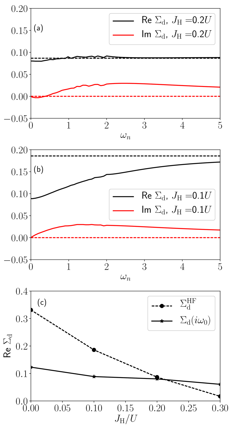
Figure 11: Difference of the self-energies $\Sigma_{\textnormal{d}}=\Sigma_{\frac{1}{2}}-\Sigma_{\frac{3}{2}}$ for $N=4$, $\lambda=0.1$, and $U=2$. Subplots (a) and (b) show $\Sigma_{\textnormal{d}}$ as a function of Matsubara frequencies $\omega_{n}$ for Hund’s couplings $J_{\textnormal{H}}=0.2\,U$ and $J_{\textnormal{H}}=0.1\,U$, respectively. The dashed lines are the corresponding Hartree-Fock values. Subplot (c) shows $\textnormal{Re}\Sigma_{\textnormal{d}}(i\omega_{0})\approx\textnormal{Re}\Sigma_{\textnormal{d}}(i\omega_{n}\rightarrow 0)$ (full line) and the Hartree-Fock values $\Sigma_{\textnormal{d}}^{\textnormal{HF}}$ equivalent to $\Sigma_{\textnormal{d}}(i\omega_{n}\rightarrow\infty)$ (dashed) as a function of $J_{\textnormal{H}}$. While the Hartree-Fock value strongly decreases with $J_{\textnormal{H}}$, $\Sigma_{\textnormal{d}}(i\omega_{0})$ is hardly influenced.

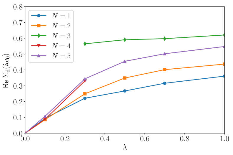
Figure 12: Increase of the first Matsubara self-energy $\Sigma_{\textnormal{d}}(i\omega_{0})\approx\Sigma_{\textnormal{d}}(\omega=0)$ with the SOC for $U=2$, $J_{\textnormal{H}}=0.1\,U$, and all integer fillings. For $N=3$ and $\lambda<0.3$, the system is a Mott insulator, and for $N=4$ and $\lambda>0.3$ a band insulator. The data points are not shown for these parameters.

Let us have a look now at the frequency dependence of the self-energy. For large frequencies, the values of $\Sigma_{\textnormal{d}}$ are given by the Hartree-Fock values. Using Eq. (8), the Hartree-Fock values in the $j$ basis are

$$\Sigma^{\textnormal{HF}}_{\frac{1}{2}}=\left<\frac{\partial H_{\textnormal{I}}}{\partial{n_{\frac{1}{2},\frac{1}{2}}}}\right> =\left(U-\frac{4}{3}J_{\textnormal{H}}\right)n_{\frac{1}{2}}$$ (28)

$$+\left(4U-\frac{26}{3}J_{\textnormal{H}}\right)n_{\frac{3}{2}}$$ (29)

$$\Sigma^{\textnormal{HF}}_{\frac{3}{2}}=\left<\frac{\partial H_{\textnormal{I}}}{\partial{n_{\frac{3}{2},\frac{3}{2}}}}\right> =\left(2U-\frac{13}{3}J_{\textnormal{H}}\right)n_{\frac{1}{2}}$$ (30)

$$+\left(3U-\frac{17}{3}J_{\textnormal{H}}\right)n_{\frac{3}{2}},$$ (31)

hence

$$\Sigma_{\textnormal{d}}(\omega\to\infty)=\Sigma_{\textnormal{d}}^{\textnormal{HF}}=\left(U-3J_{\textnormal{H}}\right)\left(n_{\frac{3}{2}}-n_{\frac{1}{2}}\right).$$ (32)

The effective SOC for large frequencies is therefore determined by an effective correlation strength $U-3J_{\textnormal{H}}$ and the orbital polarization. Since the $j=3/2$ orbital is lower in energy, its occupation is higher, and $\Sigma_{\textnormal{d}}^{\textnormal{HF}}$ is always positive as long as the effective interaction is repulsive. As a consequence, the correlations usually enhance the SOC at large frequencies.

At low frequencies and temperatures, assuming a metal, the values of $\Sigma$ are related to electronic occupancies, too. Namely, $j=1/2$ and $j=3/2$ problems are independent and the corresponding Fermi surface must, by Luttinger theorem, contain the correct number of electrons. At the Fermi surface, $\mu+\epsilon_{k}-\mathrm{Re}\Sigma=0$, which can be used to relate the difference of $\epsilon_{k}$ to the difference of $\Sigma$. Assuming that the electronic density of states is a constant $\rho$ independent of energy (square shaped function), the result is $\Sigma_{\textnormal{d}}(0)=1/\rho\left(n_{3/2}-n_{1/2}\right)-3/2\lambda$. In general, $\Sigma_{\textnormal{d}}(0)$ depends on the density of states, the SOC, and the orbital polarization, but not explicitly on the interaction parameters $U$ and $J_{\textnormal{H}}$. Since the Hartree-Fock value does depend on the interaction parameters, the large frequency and small frequency values of $\Sigma_{\textnormal{d}}$ can be quite different, as shown in Fig. 11. In contrast to the Hartree-Fock value valid at large frequencies, $\Sigma_{\textnormal{d}}(\omega=0)$ cannot be given in a closed form. However, for all metallic solutions we verified numerically that $\Sigma_{\textnormal{d}}(i\omega_{0})$ is positive, hence the effective SOC is also increased for low frequencies [41]. The results for $U=2$, $J_{\textnormal{H}}=0.1\,U$ are shown in Fig. 12.

In the case of Sr2RuO4, the DMFT work of Ref. [22] and Ref. [21] found that the real part of $\Sigma_{\textnormal{d}}$ was to a good approximation a constant and the imaginary part nearly vanishing, which motivated the introduction of $\lambda_{\mathrm{eff}}$. We reproduce this result in a DMFT calculation with parameters $N=4$, $U=2$, $J_{\textnormal{H}}=0.2\,U$, and $\lambda=0.1$, which correspond approximately to the values in Sr2RuO4. However, if the parameters are changed, for example to a Hund’s coupling of $J_{\textnormal{H}}=0.1\,U$, the off-diagonal elements of $\Sigma$ start to show a more pronounced frequency dependence, as shown in Fig. 11. The reason for this is the strong direct dependence of $\lambda_{\textnormal{eff}}$ on the interaction parameters in the Hartree-Fock limit, which is not present at low frequencies. In Fig. 11(c), one sees that the Hartree-Fock value strongly decreases with the Hund’s coupling, whereas the static value at $\omega=0$ only changes slightly. The stronger frequency dependence of $\Sigma_{\textnormal{d}}$ implies that the accuracy of describing the effects of correlations on the SOC physics in terms of $\lambda_{\textnormal{eff}}$ is in general restricted to low energies only.

References

- Imada et al. [1998] M. Imada, A. Fujimori, and Y. Tokura, Rev. Mod. Phys. 70, 1039 (1998).
- Zhou et al. [2017] Y. Zhou, K. Kanoda, and T.-K. Ng, Rev. Mod. Phys. 89, 025003 (2017).
- Nussinov and van den Brink [2015] Z. Nussinov and J. van den Brink, Rev. Mod. Phys. 87, 1 (2015).
- Jackeli and Khaliullin [2009] G. Jackeli and G. Khaliullin, Phys. Rev. Lett. 102, 017205 (2009).
- Chaloupka et al. [2010] J. c. v. Chaloupka, G. Jackeli, and G. Khaliullin, Phys. Rev. Lett. 105, 027204 (2010).
- Chen et al. [2010] G. Chen, R. Pereira, and L. Balents, Phys. Rev. B 82, 174440 (2010).
- Chen and Balents [2011] G. Chen and L. Balents, Phys. Rev. B 84, 094420 (2011).
- Meetei et al. [2015] O. N. Meetei, W. S. Cole, M. Randeria, and N. Trivedi, Phys. Rev. B 91, 054412 (2015).
- Khaliullin [2013] G. Khaliullin, Phys. Rev. Lett. 111, 197201 (2013).
- Chaloupka and Khaliullin [2015] J. c. v. Chaloupka and G. Khaliullin, Phys. Rev. B 92, 024413 (2015).
- Plumb et al. [2014] K. W. Plumb, J. P. Clancy, L. J. Sandilands, V. V. Shankar, Y. F. Hu, K. S. Burch, H.-Y. Kee, and Y.-J. Kim, Phys. Rev. B 90, 041112 (2014).
- Winter et al. [2016] S. M. Winter, Y. Li, H. O. Jeschke, and R. Valentí, Phys. Rev. B 93, 214431 (2016).
- Kim et al. [2009] B. J. Kim, H. Ohsumi, T. Komesu, S. Sakai, T. Morita, H. Takagi, and T. Arima, Science 323, 1329 (2009).
- Wang and Senthil [2011] F. Wang and T. Senthil, Phys. Rev. Lett. 106, 136402 (2011).
- Zhang et al. [2013] H. Zhang, K. Haule, and D. Vanderbilt, Phys. Rev. Lett. 111, 246402 (2013).
- Meng et al. [2014] Z. Y. Meng, Y. B. Kim, and H.-Y. Kee, Phys. Rev. Lett. 113, 177003 (2014).
- Chaloupka and Khaliullin [2016] J. c. v. Chaloupka and G. Khaliullin, Phys. Rev. Lett. 116, 017203 (2016).
- Martins et al. [2011] C. Martins, M. Aichhorn, L. Vaugier, and S. Biermann, Phys. Rev. Lett. 107, 266404 (2011).
- Martins et al. [2017] C. Martins, M. Aichhorn, and S. Biermann, Journal of Physics: Condensed Matter 29, 263001 (2017).
- Martins et al. [2018] C. Martins, B. Lenz, L. Perfetti, V. Brouet, F. m. c. Bertran, and S. Biermann, Phys. Rev. Materials 2, 032001 (2018).
- Zhang et al. [2016] G. Zhang, E. Gorelov, E. Sarvestani, and E. Pavarini, Phys. Rev. Lett. 116, 106402 (2016).
- Kim et al. [2018] M. Kim, J. Mravlje, M. Ferrero, O. Parcollet, and A. Georges, Phys. Rev. Lett. 120, 126401 (2018).
- Kim et al. [2017a] B. Kim, S. Khmelevskyi, I. Mazin, D. Agterberg, and C. Franchini, npj Quantum Materials 2, 37 (2017a).
- Mackenzie et al. [2017] A. P. Mackenzie, T. Scaffidi, C. W. Hicks, and Y. Maeno, npj Quantum Materials 2, 40 (2017).
- Haule and Kotliar [2009] K. Haule and G. Kotliar, New J. Phys. 11, 025021 (2009).
- de’ Medici et al. [2011] L. de’ Medici, J. Mravlje, and A. Georges, Physical Review Letters 107, 256401 (2011).
- Georges et al. [2013] A. Georges, L. d. Medici, and J. Mravlje, Annual Review of Condensed Matter Physics 4, 137 (2013).
- Werner et al. [2008] P. Werner, E. Gull, M. Troyer, and A. J. Millis, Phys. Rev. Lett. 101, 166405 (2008).
- Yin et al. [2012] Z. P. Yin, K. Haule, and G. Kotliar, Phys. Rev. B 86, 195141 (2012).
- Aron and Kotliar [2015] C. Aron and G. Kotliar, Phys. Rev. B 91, 041110 (2015).
- Stadler et al. [2015] K. M. Stadler, Z. P. Yin, J. von Delft, G. Kotliar, and A. Weichselbaum, Phys. Rev. Lett. 115, 136401 (2015).
- Horvat et al. [2016] A. Horvat, R. Zitko, and J. Mravlje, Phys. Rev. B 94, 165140 (2016).
- Ishida and Liebsch [2010] H. Ishida and A. Liebsch, Phys. Rev. B 81, 054513 (2010).
- Misawa et al. [2012] T. Misawa, K. Nakamura, and M. Imada, Phys. Rev. Lett. 108, 177007 (2012).
- de’ Medici et al. [2014] L. de’ Medici, G. Giovannetti, and M. Capone, Phys. Rev. Lett. 112, 177001 (2014).
- Fanfarillo and Bascones [2015] L. Fanfarillo and E. Bascones, Phys. Rev. B 92, 075136 (2015).
- Sato et al. [2015] T. Sato, T. Shirakawa, and S. Yunoki, Phys. Rev. B 91, 125122 (2015).
- Sato et al. [2016] T. Sato, T. Shirakawa, and S. Yunoki, arXiv preprint arXiv:1603.01800 (2016).
- Kim [2018] M. Kim, Phys. Rev. B 97, 155141 (2018).
- Liu et al. [2008] G.-Q. Liu, V. N. Antonov, O. Jepsen, and O. K. Andersen., Phys. Rev. Lett. 101, 026408 (2008).
- Bünemann et al. [2016] J. Bünemann, T. Linneweber, U. Löw, F. B. Anders, and F. Gebhard, Phys. Rev. B 94, 035116 (2016).
- Behrmann et al. [2012] M. Behrmann, C. Piefke, and F. Lechermann, Phys. Rev. B 86, 045130 (2012).
- Horvat et al. [2017] A. Horvat, R. Zitko, and J. Mravlje, Phys. Rev. B 96, 085122 (2017).
- Kim et al. [2017b] A. J. Kim, H. O. Jeschke, P. Werner, and R. Valentí, Phys. Rev. Lett. 118, 086401 (2017b).
- Piefke and Lechermann [2018] C. Piefke and F. Lechermann, Phys. Rev. B 97, 125154 (2018).
- Facio et al. [2018] J. I. Facio, J. Mravlje, L. Pourovskii, P. S. Cornaglia, and V. Vildosola, Phys. Rev. B 98, 085121 (2018).
- Sugano et al. [1970] S. Sugano, Y. Tanabe, and H. Kamimura, Multiplets of transition-metal ions in crystals, Pure and Applied Physics, Vol. 33 (Academic Press, New York, 1970).
- Georges et al. [1996] A. Georges, G. Kotliar, W. Krauth, and M. J. Rozenberg, Rev. Mod. Phys. 68, 13 (1996).
- Metzner and Vollhardt [1989] W. Metzner and D. Vollhardt, Phys. Rev. Lett. 62, 324 (1989).
- Werner and Millis [2006] P. Werner and A. J. Millis, Phys. Rev. B 74, 155107 (2006).
- Parcollet et al. [2015] O. Parcollet, M. Ferrero, T. Ayral, H. Hafermann, I. Krivenko, L. Messio, and P. Seth, Computer Physics Communications 196, 398 (2015).
- Seth et al. [2016] P. Seth, I. Krivenko, M. Ferrero, and O. Parcollet, Comput. Phys. Commun. 200, 274 (2016).
- Kaushal et al. [2017] N. Kaushal, J. Herbrych, A. Nocera, G. Alvarez, A. Moreo, F. A. Reboredo, and E. Dagotto, Phys. Rev. B 96, 155111 (2017).
- Kunes [2015] J. Kunes, Journal of Physics: Condensed Matter 27, 333201 (2015).
- Akbari and Khaliullin [2014] A. Akbari and G. Khaliullin, Phys. Rev. B 90, 035137 (2014).
- Kim et al. [2016] B. Kim, P. Liu, Z. Ergönenc, A. Toschi, S. Khmelevskyi, and C. Franchini, Phys. Rev. B 94, 241113 (2016).
- Du et al. [2013a] L. Du, L. Huang, and X. Dai, The European Physical Journal B 86, 94 (2013a).
- Werner and Millis [2007] P. Werner and A. J. Millis, Physical Review Letters 99, 126405 (2007).
- Werner et al. [2009] P. Werner, E. Gull, and A. J. Millis, Physical Review B 79, 115119 (2009).
- Kita et al. [2011a] T. Kita, T. Ohashi, and N. Kawakami, Physical Review B 84, 195130 (2011a).
- Kita et al. [2011b] T. Kita, T. Ohashi, and N. Kawakami, Journal of the Physical Society of Japan 80, SA142 (2011b).
- Jarrell and Gubernatis [1996] M. Jarrell and J. Gubernatis, Physics Reports 269, 133 (1996).
- von der Linden et al. [1999] W. von der Linden, R. Preuss, and V. Dose, “The Prior-Predictive Value: A Paradigm of Nasty Multi-Dimensional Integrals,” in Maximum Entropy and Bayesian Methods, edited by W. von der Linden, V. Dose, R. Fischer, and R. Preuss (Kluwer Academic Publishers, Dortrecht, 1999) pp. 319–326.
- Skilling [1991] J. Skilling, “Fundamentals of MaxEnt in data analysis,” in Maximum Entropy in Action, edited by B. Buck and V. A. Macaulay (Clarendon Press, Oxford, 1991) pp. 19–40.
- Montalti et al. [2006] M. Montalti, A. Credi, L. Prodi, and M. T. Gandolfi, Handbook of Photochemistry, 3rd ed. (CRC press, 2006).
- Lee and Pickett [2007] K.-W. Lee and W. E. Pickett, EPL (Europhysics Letters) 80, 37008 (2007).
- Giovannetti [2016] G. Giovannetti, arXiv preprint arXiv:1611.06482 (2016).
- Shi et al. [2009] Y. G. Shi, Y. F. Guo, S. Yu, M. Arai, A. A. Belik, A. Sato, K. Yamaura, E. Takayama-Muromachi, H. F. Tian, H. X. Yang, J. Q. Li, T. Varga, J. F. Mitchell, and S. Okamoto, Phys. Rev. B 80, 161104 (2009).
- Ikeda et al. [2000] S.-I. Ikeda, N. Shirakawa, H. Bando, and Y. Ootuka, Journal of the Physical Society of Japan 69, 3162 (2000).
- Nagai et al. [2005] I. Nagai, N. Shirakawa, S.-i. Ikeda, R. Iwasaki, H. Nishimura, and M. Kosaka, Applied Physics Letters 87, 024105 (2005).
- Wadati et al. [2014] H. Wadati, J. Mravlje, K. Yoshimatsu, H. Kumigashira, M. Oshima, T. Sugiyama, E. Ikenaga, A. Fujimori, A. Georges, A. Radetinac, K. S. Takahashi, M. Kawasaki, and Y. Tokura, Phys. Rev. B 90, 205131 (2014).
- Du et al. [2013b] L. Du, X. Sheng, H. Weng, and X. Dai, EPL (Europhysics Letters) 101, 27003 (2013b).