Theoretical study of the $\Delta^{++}-\Delta^{-}$ configuration in the deuteron using antiproton beam

Abstract

We study the manifestation of the $\Delta^{++}-\Delta^{-}$ component of the deuteron wave function in the exclusive reaction $\bar{p}d\to\pi^{-}\pi^{-}\Delta^{++}$. Due to the large binding energy the internal motion in the $\Delta-\Delta$ system is relativistic. We take this into account within the light-cone (LC) wave function formalism and, indeed, found large differences between calculations based on the LC and non-relativistic (NR) wave functions. We demonstrate, that the consistent LC treatment of the $\Delta-\Delta$ system plays the key role in the separation of the signal and background. Within the LC approach, the characteristic shape of the momentum distribution of the $\Delta-\Delta$ bound system predicted by the meson-exchange model is well visible on the background of usual annihilations at beam momenta between 10 and 15 GeV/c.

1 Introduction

One of the hottest fields of the modern nuclear physics is the study of non-nucleonic degrees-of-freedom in nuclei. This issue is closely related to the mechanism of hadronic interactions at short distances where the partonic structure of hadrons becomes important. As the lightest nucleus, the deuteron is an ideal object for testing theoretical models of non-nucleonic degrees-of-freedom. In this case angular momentum and isospin conservation allow to considerably reduce the space of possible exotic configurations and simplify the physical picture. In particular, the lightest exotic baryonic configuration is a mixture of $\Delta^{++}-\Delta^{-}$ and $\Delta^{+}-\Delta^{0}$ states with equal probabilities. There is a substantial difference in various theoretical predictions on the $\Delta-\Delta$ component of the deuteron.

In the meson-exchange calculations of the deuteron Haapakoski and Saarela (1974); Arenhövel (1975); Dymarz and Khanna (1990); Haidenbauer et al. (1993), the short-range structure of the $NN\rightarrow\Delta\Delta$ transition potential has been effectively described by inserting the cut off (hard core radius) in the pion-exchange potential and adding $\rho$ meson exchange Haapakoski and Saarela (1974) or using formfactors Arenhövel (1975); Dymarz and Khanna (1990); Haidenbauer et al. (1993) in meson-nucleon-delta vertices. In most calculations, the ${}^{7}D_{1}$ state dominates in the $\Delta-\Delta$ wave function. The ${}^{3}S_{1}^{NN}\to\>^{7}D_{1}^{\Delta\Delta}$ transition is driven by the tensor interaction due to $\pi$ and $\rho$ exchanges which contribute with opposite signs. Thus, at short distances, the inclusion of $\rho$ exchange has been shown to be very important, as it stabilizes the cut-off dependence of the results Haapakoski and Saarela (1974). The meson-exchange calculations typically predict that the deuteron has a $\Delta-\Delta$ component with a probability $<1.5\%$.

The typical momenta in the $\Delta-\Delta$ wave function are $\sim 400\div 500$ MeV/c (see Fig. 2). This corresponds to the inter-$\Delta$ distances $\sim\pi/2k\sim 0.6\div 0.8$ fm which are much smaller than the root-mean-square radius of the ordinary deuteron $\sim 2$ fm. Thus, the $\Delta-\Delta$ wave function has a strong overlap with other non-nucleonic configurations such as e.g. six quark states which one can try to model. For example, in the constituent quark model calculations with oscillator basis Glozman et al. (1993); Glozman and Kuchina (1994) the main contribution to the $\Delta-\Delta$ wave function is due to the $s^{6}$ quark configuration. Thus, the $\Delta-\Delta$ configuration is described by the $0s$ oscillator state. This model predicts the probability of the $\Delta-\Delta$ component to be $\sim 2-3\%$.

Experimentally, the $\Delta-\Delta$ component has been already discussed in previous analyses of photon Benz and Soding (1974) and antiproton Braun et al. (1974) reactions on the deuteron. In ref. Benz and Soding (1974), DESY data on backward $\Delta^{++}$ production in the laboratory (lab.) frame in the reaction $\gamma d\to\Delta^{++}+{\rm anything}$ were analyzed deducing $\sim 3\%$ $\Delta-\Delta$ admixture in the deuteron. In ref. Braun et al. (1974), non-annihilative channels of $\bar{p}d$ interactions have been used for the search of the $\Delta-\Delta$ component. The high percentage of $\sim 16\%$ of the $\Delta-\Delta$ component deduced in ref. Braun et al. (1974) strongly indicates that the background was not fully excluded in the spectator $\Delta$ decays in the backward hemisphere in the lab. frame. An upper limit of 0.4% on the $\Delta-\Delta$ component has been obtained in $\nu(\bar{\nu})d$ interaction studies Allasia et al. (1986), where the neutrino (antineutrino) was supposed to interact with the quark content of $\Delta^{-}(\Delta^{++})$ leaving the $\Delta^{++}(\Delta^{-})$ as a low-momentum spectator.

In the OBELIX@LEAR experiment Bertin et al. (1997) the reaction

$$\bar{p}d\to 2\pi^{-}\pi^{+}p$$ (1)

with stopped antiprotons was used to estimate an upper limit on the annihilation probability $Y_{\bar{p}(\Delta^{-}\Delta^{++})\to 2\pi^{-}\pi^{+}p}$ due to the subprocess $\bar{p}\Delta^{-}\to\pi^{-}\pi^{-}$. The resulting $Y_{\bar{p}(\Delta^{-}\Delta^{++})\to 2\pi^{-}\pi^{+}p}\leq 6.5\times 10^{-5}$ corresponds to a $\Delta-\Delta$ configuration probability $\leq 1\%$. In ref. Denisov et al. (1999) some enhancement in the invariant mass distribution of $\pi^{-}\pi^{-}$ pairs at 1.4-1.5 GeV from reaction (1) visible in the OBELIX data Bertin et al. (1997) was interpreted by including the $\Delta^{-}\Delta^{++}$ component. However, due to the lack of statistics it is difficult to make definite conclusions on the existence of a $\Delta-\Delta$ component from the OBELIX data.

In the present paper – in view of the upcoming PANDA experiment – we theoretically address the reaction channel $\bar{p}d\to\pi^{-}\pi^{-}\Delta^{++}$ at $p_{\rm lab}=10\div 15$ GeV/c for the kinematics with two energetic $\pi^{-}$ mesons in the forward lab. hemisphere and a slow $\Delta^{++}$. The “signal” reaction channel is $\bar{p}\Delta^{-}\to\pi^{-}\pi^{-}$ annihilation on the virtual $\Delta^{-}$ leading to a practically instantaneous (on nuclear scale) release of the spectator $\Delta^{++}$. The possible background channels include at least two steps and, thus, are expected to be moderate. We will consider the following two possible background reactions: (i) $\bar{p}n\to\pi^{-}\pi^{0}$ followed by the charge exchange (CEX) reaction $\pi^{0}p\to\pi^{-}\Delta^{++}$ and (ii) $\bar{p}n\to\pi^{-}\pi^{-}\pi^{+}$ followed by $\pi^{+}p\to\Delta^{++}$.

The other isospin component, i.e. $\Delta^{+}\Delta^{0}$, can be studied in the $\bar{p}d\to\pi^{-}\pi^{+}\Delta^{0}$ channel. However, background of the types (i) and (ii) will in this case include the annihilation channels both on the proton and on the neutron, and thus presumably will be larger. Therefore, for simplicity, we restrict ourselves in this work to the analysis of $\bar{p}$ annihilation on the $\Delta^{++}\Delta^{-}$ component.

In calculations of the signal channel we use both NR and LC descriptions of the $\Delta-\Delta$ wave function and analyze their influence on the results. Both NR and LC descriptions are based on the same input $\Delta-\Delta$ momentum distribution provided by calculations based on the model of ref. Haidenbauer et al. (1993), but differ in the physical meaning of the intrinsic $\Delta-\Delta$ momentum. The elementary two-pion annihilation amplitudes are calculated in the framework of the nucleon- and $\Delta$-exchange model. The CEX $\pi^{0}p\to\pi^{-}\Delta^{++}$ amplitude is described by the reggeized $\rho$ exchange. We show that LC effects are strong in case of a strongly bound $\Delta-\Delta$ configuration and crucial for the visibility of the signal which is comparable in strength with the three-pion annihilation background in the backward lab. hemisphere.

The structure of the paper is as follows. In sect. 2 we derive the signal cross section in the NR and LC descriptions. In sect. 3, the wave function of the $\Delta-\Delta$ state used in the calculations is described briefly. Section 4 includes the formalism for the calculation of the background channels. Section 5 contains numerical results. Finally, in sect. 6 we summarize the results and try to draw conclusions on the possibility to observe the $\Delta-\Delta$ component of the deuteron experimentally.

The appendices contain some technical aspects. In Appendix A we derive the relation between the NR and LC $\Delta-\Delta$ wave functions based on the electromagnetic formfactor of the $\Delta-\Delta$ state. In Appendix B we obtain Eq.(102) for the poles of the pion propagator used in the calculation of the three-pion annihilation background in sect. 4.2. The elementary amplitudes are described in Appendix C.

2 Antiproton interaction with a deuteron $\Delta$-$\Delta$ configuration

We will start from the detailed NR derivation and then sketch the main steps of the LC derivation. In the latter case more details can be found in refs. Frankfurt and Strikman (1979, 1981).

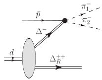
Figure 1: Impulse approximation graph showing the production of a pion pair in antiproton annihilation on one of the $\Delta$’s of a $\Delta$-$\Delta$ configuration in the deuteron.

The $S$-matrix corresponding to the Feynman diagram of Fig. 1 can be written as follows:

$$S^{(0)}=\int d^{3}r_{\Delta_{R}}d^{3}r_{\Delta}\sum_{\lambda_{\Delta}}\phi_{\Delta-\Delta}^{\lambda_{d}}(\bm{r}_{\Delta_{R}},\bm{r}_{\Delta};\lambda_{\Delta_{R}},\lambda_{\Delta})\frac{1}{V}\int\frac{Vd^{3}p_{\Delta}}{(2\pi)^{3}}e^{-i\bm{p}_{\Delta_{R}}\bm{r}_{\Delta_{R}}-i\bm{p}_{\Delta}\bm{r}_{\Delta}}S_{\pi_{1}\pi_{2};\bar{p}\Delta}~{},$$ (2)

where

$$S_{\pi_{1}\pi_{2};\bar{p}\Delta}=\frac{(2\pi)^{4}\delta^{(4)}(p_{1}+p_{2}-p_{\bar{p}}-p_{\Delta})}{(2E_{\bar{p}}V2E_{\Delta}V2E_{1}V2E_{2}V)^{1/2}}iM_{\pi_{1}\pi_{2};\bar{p}\Delta}$$ (3)

is the $S$-matrix corresponding to the process $\bar{p}\Delta\to\pi_{1}\pi_{2}$. $V$ is a normalization volume. $\phi_{\Delta-\Delta}^{\lambda_{d}}(\bm{r}_{\Delta_{R}},\bm{r}_{\Delta};\lambda_{\Delta_{R}},\lambda_{\Delta})$ is the wave function of the $\Delta$-$\Delta$ configuration normalized according to the following condition:

$$\sum_{\lambda_{\Delta_{R}},\lambda_{\Delta}}\int d^{3}r_{\Delta_{R}}d^{3}r_{\Delta}|\phi_{\Delta-\Delta}^{\lambda_{d}}(\bm{r}_{\Delta_{R}},\bm{r}_{\Delta};\lambda_{\Delta_{R}},\lambda_{\Delta})|^{2}=P_{\Delta-\Delta}~{},$$ (4)

where $P_{\Delta-\Delta}$ is the probability of a $\Delta$-$\Delta$ configuration in the deuteron. $\lambda_{d}$, $\lambda_{\Delta_{R}}$ and $\lambda_{\Delta}$ are the third spin components of the deuteron, residual and struck $\Delta$’s, respectively.

By using the center-of-mass (c.m.), $\bm{R}$, and relative, $\bm{r}$, coordinates,

$$\bm{R}=\frac{m_{\Delta}\bm{r}_{\Delta}+m_{\Delta_{R}}\bm{r}_{\Delta_{R}}}{m_{\Delta}+m_{\Delta_{R}}}~{},~{}~{}~{}\bm{r}=\bm{r}_{\Delta}-\bm{r}_{\Delta_{R}}~{},$$ (5)

one can separate the c.m. motion and relative motion in the wave function as follows:

$$\phi_{\Delta-\Delta}^{\lambda_{d}}(\bm{r}_{\Delta_{R}},\bm{r}_{\Delta};\lambda_{\Delta_{R}},\lambda_{\Delta})=\frac{1}{\sqrt{V}}e^{i\bm{p}_{d}\bm{R}}\phi_{\Delta-\Delta}(\bm{r};\lambda_{\Delta_{R}},\lambda_{\Delta})~{}.$$ (6)

Substituting Eqs.(3),(6) in Eq.(2) and integrating-out the c.m. motion we have:

$$S^{(0)} = \int d^{3}r\sum_{\lambda_{\Delta}}\frac{1}{\sqrt{V}}\phi_{\Delta-\Delta}^{\lambda_{d}}(\bm{r};\lambda_{\Delta_{R}},\lambda_{\Delta})\int d^{3}p_{\Delta}\delta^{(3)}(\bm{p}_{d}-\bm{p}_{\Delta_{R}}-\bm{p}_{\Delta})$$ (7)

$$\times e^{i(\bm{p}_{\Delta_{R}}m_{\Delta}-\bm{p}_{\Delta}m_{\Delta_{R}})\bm{r}/(m_{\Delta}+m_{\Delta_{R}})}\,\frac{(2\pi)^{4}\delta^{(4)}(p_{1}+p_{2}-p_{\bar{p}}-p_{\Delta})}{(2E_{\bar{p}}V2E_{\Delta}V2E_{1}V2E_{2}V)^{1/2}}iM_{\pi_{1}\pi_{2};\bar{p}\Delta}~{}.$$

If one defines the energy of the struck $\Delta$ as

$$E_{\Delta}=E_{d}-E_{\Delta_{R}}~{},$$ (8)

then, integrating-out the first $\delta$-function in Eq.(7), we can finally express the $S$-matrix in the standard form,

$$S^{(0)}=\frac{(2\pi)^{4}\delta^{(4)}(p_{1}+p_{2}+p_{\Delta_{R}}-p_{\bar{p}}-p_{d})}{(2E_{\bar{p}}V2E_{d}V2E_{\Delta_{R}}V2E_{1}V2E_{2}V)^{1/2}}\,iM_{\pi_{1}\pi_{2}\Delta_{R};\bar{p}d}^{(0)}~{},$$ (9)

where the invariant matrix element is given by the following expression:

$$M_{\pi_{1}\pi_{2}\Delta_{R};\bar{p}d}^{(0)}=\left(\frac{2E_{\Delta_{R}}E_{d}}{E_{\Delta}}\right)^{1/2}(2\pi)^{3/2}\sum_{\lambda_{\Delta}}\phi_{\Delta-\Delta}^{\lambda_{d}}(\bm{k};\lambda_{\Delta_{R}},\lambda_{\Delta})M_{\pi_{1}\pi_{2};\bar{p}\Delta}~{},$$ (10)

where

$$\bm{k}=-\bm{p}_{\Delta_{R}}+\frac{m_{\Delta_{R}}\bm{p}_{d}}{m_{\Delta}+m_{\Delta_{R}}}$$ (11)

is the momentum of the struck $\Delta$ . The wave function in momentum space is defined as follows:

$$\phi_{\Delta-\Delta}^{\lambda_{d}}(\bm{k};\lambda_{\Delta_{R}},\lambda_{\Delta})=\frac{1}{(2\pi)^{3/2}}\int d^{3}re^{-i\bm{k}\bm{r}}\phi_{\Delta-\Delta}^{\lambda_{d}}(\bm{r};\lambda_{\Delta_{R}},\lambda_{\Delta})~{}.$$ (12)

The normalization condition for this wave function is

$$\sum_{\lambda_{\Delta_{R}},\lambda_{\Delta}}\int d^{3}k|\phi_{\Delta-\Delta}^{\lambda_{d}}(\bm{k};\lambda_{\Delta_{R}},\lambda_{\Delta})|^{2}=P_{\Delta-\Delta}~{}.$$ (13)

Note that based on Eq.(10) one can obtain the relation between the deuteron vertex function $d\to\Delta\Delta$ and the wave function of the $\Delta-\Delta$ state (cf. ref. Frankfurt et al. (1997)):

$$\frac{i\Gamma_{d\to\Delta\Delta}(p_{d},p_{\Delta_{R}};\lambda_{d},\lambda_{\Delta_{R}},\lambda_{\Delta})}{p_{\Delta}^{2}-m_{\Delta}^{2}+i\epsilon}=\left(\frac{2E_{\Delta_{R}}E_{d}}{E_{\Delta}}\right)^{1/2}(2\pi)^{3/2}\phi_{\Delta-\Delta}^{\lambda_{d}}(\bm{k};\lambda_{\Delta_{R}},\lambda_{\Delta})~{}.$$ (14)

In the deuteron rest frame (lab. frame) the differential cross section of the process shown in Fig. 1 is

$$d\sigma=\frac{(2\pi)^{4}\delta^{(4)}(p_{1}+p_{2}+p_{\Delta_{R}}-p_{\bar{p}}-p_{d})}{4m_{d}p_{\rm lab}}\overline{|M_{\pi_{1}\pi_{2}\Delta_{R};\bar{p}d}^{(0)}|^{2}}\frac{d^{3}p_{\Delta_{R}}}{(2\pi)^{3}2E_{\Delta_{R}}}\frac{d^{3}p_{1}}{(2\pi)^{3}2E_{1}}\frac{d^{3}p_{2}}{(2\pi)^{3}2E_{2}}~{},$$ (15)

where $\overline{|M_{\pi_{1}\pi_{2}\Delta_{R};\bar{p}d}^{(0)}|^{2}}$ is the modulus squared of the invariant matrix element, Eq.(10), summed over final spins and averaged over initial spins.

For the modulus squared of the invariant matrix element in the lab. frame we have:

$$\overline{|M_{\pi_{1}\pi_{2}\Delta_{R};\bar{p}d}^{(0)}|^{2}} = \frac{1}{6}\sum_{\lambda_{\bar{p}},\lambda_{d},\lambda_{\Delta_{R}}}|M_{\pi_{1}\pi_{2}\Delta_{R};\bar{p}d}^{(0)}|^{2}=\frac{2E_{\Delta_{R}}m_{d}}{E_{\Delta}}\frac{(2\pi)^{3}}{6}$$ (16)

$$\times\sum_{\lambda_{\bar{p}},\lambda_{d},\lambda_{\Delta_{R}}}\sum_{\lambda_{\Delta},\lambda_{\Delta}^{\prime}}\phi_{\Delta-\Delta}^{\lambda_{d}}(\bm{k};\lambda_{\Delta_{R}},\lambda_{\Delta}){\phi_{\Delta-\Delta}^{\lambda_{d}}}^{*}(\bm{k};\lambda_{\Delta_{R}},\lambda_{\Delta}^{\prime})M_{\pi_{1}\pi_{2};\bar{p}\Delta}M^{*}_{\pi_{1}\pi_{2};\bar{p}\Delta^{\prime}}$$

$$= \frac{2E_{\Delta_{R}}m_{d}}{E_{\Delta}}\frac{(2\pi)^{3}}{6}\sum_{\lambda_{\bar{p}},\lambda_{d},\lambda_{\Delta_{R}},\lambda_{\Delta}}|\phi_{\Delta-\Delta}^{\lambda_{d}}(\bm{k};\lambda_{\Delta_{R}},\lambda_{\Delta})|^{2}\,|M_{\pi_{1}\pi_{2};\bar{p}\Delta}|^{2}~{},$$

where in the last step we neglected the interference terms between transitions with different spin projections of the struck $\Delta$. Neglecting the spin dependence of the transition probability $\bar{p}\Delta\to\pi_{1}\pi_{2}$, we can replace $|M_{\pi_{1}\pi_{2};\bar{p}\Delta}|^{2}$ by its averaged value over the third spin components of $\bar{p}$ and $\Delta$, $\overline{|M_{\pi_{1}\pi_{2};\bar{p}\Delta}|^{2}}$. This allows to simplify Eq.(16) to the following form:

$$\overline{|M_{\pi_{1}\pi_{2}\Delta_{R};\bar{p}d}^{(0)}|^{2}}=\frac{2E_{\Delta_{R}}m_{d}}{E_{\Delta}}(2\pi)^{3}|\phi_{\Delta-\Delta}(\bm{k})|^{2}\,\overline{|M_{\pi_{1}\pi_{2};\bar{p}\Delta}|^{2}}~{},$$ (17)

where the deuteron-spin-averaged modulus squared of the $\Delta-\Delta$ wave function,

$$|\phi_{\Delta-\Delta}(\bm{k})|^{2}\equiv\frac{1}{3}\sum_{\lambda_{d},\lambda_{\Delta_{R}},\lambda_{\Delta}}|\phi_{\Delta-\Delta}^{\lambda_{d}}(\bm{k};\lambda_{\Delta_{R}},\lambda_{\Delta})|^{2}~{},$$ (18)

describes the momentum distribution of $\Delta_{R}$ in the $\Delta$-$\Delta$ configuration. It is normalized as

$$\int d^{3}k|\phi_{\Delta-\Delta}(\bm{k})|^{2}=P_{\Delta-\Delta}~{}.$$ (19)

Substituting Eq.(17) in Eq.(15) we have

$$d\sigma = \frac{(2\pi)^{4}\delta^{(4)}(p_{1}+p_{2}+p_{\Delta_{R}}-p_{\bar{p}}-p_{d})}{4p_{\rm lab}E_{\Delta}}\,|\phi_{\Delta-\Delta}(\bm{k})|^{2}\,$$ (20)

$$\times\overline{|M_{\pi_{1}\pi_{2};\bar{p}\Delta}|^{2}}\,\frac{d^{3}p_{1}}{(2\pi)^{3}2E_{1}}\frac{d^{3}p_{2}}{(2\pi)^{3}2E_{2}}d^{3}p_{\Delta_{R}}~{}.$$

This equation can be further simplified by using the elementary differential cross section

$$d\sigma_{\bar{p}\Delta\to\pi_{1}\pi_{2}}=\frac{(2\pi)^{4}\delta^{(4)}(p_{1}+p_{2}-p_{\bar{p}}-p_{\Delta})}{4I_{\bar{p}\Delta}}\overline{|M_{\pi_{1}\pi_{2};\bar{p}\Delta}|^{2}}\frac{d^{3}p_{1}}{(2\pi)^{3}2E_{1}}\frac{d^{3}p_{2}}{(2\pi)^{3}2E_{2}}~{},$$ (21)

where

$$I_{\bar{p}\Delta}=\sqrt{(p_{\bar{p}}p_{\Delta})^{2}-m_{\bar{p}}^{2}\tilde{m}_{\Delta}^{2}}$$ (22)

is the Möller flux factor,

$$p_{\bar{p}} = (E_{\bar{p}},0,0,p_{\rm lab})$$ (23)

$$p_{\Delta} = p_{d}-p_{\Delta_{R}}=(E_{\Delta},\bm{k})$$ (24)

are the four-momenta of the incoming antiproton and of the struck $\Delta$, respectively, and

$$\tilde{m}_{\Delta}^{2}=p_{\Delta}^{2}=(E_{\Delta})^{2}-\bm{k}^{2}$$ (25)

is the (off-shell) invariant mass of the struck $\Delta$.

Thus, using Eq.(21) we can rewrite Eq.(20) as

$$d\sigma=\frac{E_{\bar{p}}}{p_{\rm lab}}v_{\bar{p}\Delta}|\phi_{\Delta-\Delta}(\bm{k})|^{2}d\sigma_{\bar{p}\Delta\to\pi_{1}\pi_{2}}d^{3}p_{\Delta_{R}}~{},$$ (26)

where

$$v_{\bar{p}\Delta}=\frac{I_{\bar{p}\Delta}}{E_{\bar{p}}E_{\Delta}}$$ (27)

is the relative velocity of the antiproton and the struck $\Delta$. Using the invariant

$$t=(p_{1}-p_{\bar{p}})^{2}$$ (28)

we obtain

$$\frac{d^{4}\sigma}{d^{3}p_{\Delta_{R}}dt}=\frac{E_{\bar{p}}}{p_{\rm lab}}v_{\bar{p}\Delta}|\phi_{\Delta-\Delta}(\bm{k})|^{2}\frac{d\sigma_{\bar{p}\Delta\to\pi_{1}\pi_{2}}(s^{\prime},t)}{dt}~{},$$ (29)

where $s^{\prime}=(p_{\bar{p}}+p_{d}-p_{\Delta_{R}})^{2}$. The kinematic prefactor in Eq.(29) can be explicitly calculated as follows:

$$\frac{E_{\bar{p}}}{p_{\rm lab}}v_{\bar{p}\Delta}=\frac{I_{\bar{p}\Delta}}{p_{\rm lab}E_{\Delta}}=\frac{\sqrt{(E_{\bar{p}}E_{\Delta}-p_{\rm lab}k^{z})^{2}-m_{\bar{p}}^{2}\tilde{m}_{\Delta}^{2}}}{p_{\rm lab}E_{\Delta}}~{},$$ (30)

where $E_{\bar{p}}=\sqrt{m_{\bar{p}}^{2}+p_{\rm lab}^{2}}$, $E_{\Delta}=m_{d}-E_{\Delta_{R}}$, $E_{\Delta_{R}}=\sqrt{m_{\Delta_{R}}^{2}+\bm{p}_{\Delta_{R}}^{2}}$. We recall that $\bm{k}=-\bm{p}_{\Delta_{R}}$ in Eqs.(29),(30) since these equations are obtained treating the deuteron non-relativistically.

One can formally express the kinematic prefactors in Eq.(29) in terms of the light cone variable

$$\alpha=\frac{E_{\Delta_{R}}-p_{\Delta_{R}}^{z}}{m_{d}/2}~{},$$ (31)

as defined in the deuteron rest frame. Hence, $\alpha/2$ is the fraction of deuteron momentum carried by $\Delta_{R}$ in the infinite momentum frame (where $\Delta_{R}$ moves fast in negative $z$ direction). We have also

$$2-\alpha=\frac{E_{\Delta}-k^{z}}{m_{d}/2}~{}.$$ (32)

In the limit of very high beam momenta such that $p_{\rm lab}\simeq E_{\bar{p}}$ one can neglect masses in the Möller flux factor Eq.(22):

$$I_{\bar{p}\Delta}\simeq p_{\bar{p}}p_{\Delta}\simeq p_{\rm lab}(E_{\Delta}-k^{z})=p_{\rm lab}\frac{m_{d}}{2}(2-\alpha)~{}.$$ (33)

This leads to the relative velocity

$$v_{\bar{p}\Delta}\simeq\frac{m_{d}/2}{E_{\Delta}}(2-\alpha)~{}.$$ (34)

Using Eq.(34) we can rewrite the differential cross section (29) as

$$\frac{d^{4}\sigma}{d^{3}p_{\Delta_{R}}dt}=\frac{m_{d}/2}{E_{\Delta}}(2-\alpha)|\phi_{\Delta-\Delta}(\bm{k})|^{2}\frac{d\sigma_{\bar{p}\Delta\to\pi_{1}\pi_{2}}(s^{\prime},t)}{dt}~{},$$ (35)

where

$$s^{\prime}=(p_{\bar{p}}+p_{d}-p_{\Delta_{R}})^{2}=(p_{\bar{p}}+p_{\Delta})^{2}\simeq 2p_{\bar{p}}p_{\Delta}\simeq p_{\rm lab}m_{d}(2-\alpha)~{}.$$ (36)

If we define the invariant energy squared for the antiproton collision with a nucleon at rest

$$s\equiv(p_{\bar{p}}+p_{N})^{2}=2E_{\bar{p}}m_{N}+2m_{N}^{2}~{},$$ (37)

then we have

$$s^{\prime}\simeq s(2-\alpha)~{}.$$ (38)

We stress that Eq.(35) is simply the high-energy limit of Eq.(29).

The problematic feature of the derivation given above is that the contribution of the baryon-antibaryon pairs is included in the NR wave function in an uncontrolled way. This results in the finite value of $|\phi_{\Delta-\Delta}(\bm{k})|^{2}$ at $\alpha>2$. This problem can be solved within the LC formalism. It is clear that the baryon-antibaryon pairs, i.e. vacuum fluctuations, should not contribute to the LC wave function since it is evaluated in the frame where the deuteron is fast, and thus the time scale of its internal dynamics is slowed down Frankfurt and Strikman (1979, 1981).

Thus, in the LC formalism one should evaluate the graph of Fig. 1 within the non-covariant perturbation theory (time from left to right) and perform the transformation of the result in the infinite momentum frame where another graph (not shown) with the emission of an antidelta from the antiproton disappears. The calculation is almost identical to that for photon absorption in ref. Frankfurt and Strikman (1979). Thus, we will not repeat it here and only show the final result:

$$E_{\Delta_{R}}\frac{d^{4}\sigma}{d^{3}p_{\Delta_{R}}dt}=\left|\frac{\Gamma_{d\to\Delta\Delta}(p_{d},p_{\Delta_{R}})}{(2-\alpha)(m_{d}^{2}-M_{\Delta,\Delta_{R}}^{2})}\right|^{2}\frac{(2-\alpha)}{(2\pi)^{3}}\frac{d\sigma_{\bar{p}\Delta\to\pi_{1}\pi_{2}}(s^{\prime},t)}{dt}~{}.$$ (39)

Here, $M_{\Delta,\Delta_{R}}^{2}$ is the invariant mass of the intermediate $\Delta-\Delta$ state expressed as

$$M_{\Delta,\Delta_{R}}^{2}=\frac{4(m_{\Delta}^{2}+p_{\Delta_{R}t}^{2})}{\alpha(2-\alpha)}=4(m_{\Delta}^{2}+\bm{k}^{2})~{},$$ (40)

where on the last step we inserted a new variable conveniently used in the LC formalism (cf. Frankfurt and Strikman (1979, 1981) and Appendix A), the internal momentum $\bm{k}$ defined by relations

$$\alpha=1+\frac{k^{z}}{\sqrt{m_{\Delta}^{2}+\bm{k}^{2}}}~{},~{}~{}~{}\bm{k}_{t}=-\bm{p}_{\Delta_{R}t}~{},$$ (41)

where $\alpha$ is related to the residual $\Delta$ momentum via Eq.(31). Using Eqs.(86),(92) of Appendix A, the following expression for the differential cross section can be obtained:

$$E_{\Delta_{R}}\frac{d^{4}\sigma}{d^{3}p_{\Delta_{R}}dt}=\frac{m_{d}/2}{m_{d}-m_{\Delta}}\frac{|\phi_{\Delta-\Delta}(\bm{k})|^{2}}{2-\alpha}\sqrt{m_{\Delta}^{2}+\bm{k}^{2}}\frac{d\sigma_{\bar{p}\Delta\to\pi_{1}\pi_{2}}(s^{\prime},t)}{dt}~{},$$ (42)

where $m_{\Delta}$ is the physical mass of the residual $\Delta$.

3 Wave function of the $\Delta-\Delta$ system

The $\Delta-\Delta$ component of the deuteron wave function is a superposition of the ${}^{3}S_{1},~{}^{3}D_{1},~{}^{7}D_{1}$, and ${}^{7}G_{1}$ states. In our calculations we applied the wave functions of the $np$ and $\Delta-\Delta$ systems according to the coupled-channel folded-diagram potential (CCF) model of ref. Haidenbauer et al. (1993). This model has been primarily developed for the description of many-body systems as the resulting two-body potential is energy-independent which substantially simplifies calculations. The two-body observables ($NN$ phase shifts, deuteron properties) are reproduced with an accuracy comparable to that of the (energy-dependent) full Bonn potential Machleidt et al. (1987). Indeed, the analytic expressions for the meson-baryon vertex functions are identical to those of the Bonn potential. The numerical values of the meson-nucleon coupling constants and cutoff masses are, however, readjusted by a best fit to the empirical $NN$ phase shifts. The CCF model is defined in momentum space and thus we start directly from the momentum space representation.

The $\Delta-\Delta$ wave function in momentum space, Eq.(12), can be represented in the $LS$ basis as follows:

$$\phi_{\Delta-\Delta}^{\lambda_{d}}(\bm{k};\lambda_{\Delta_{R}},\lambda_{\Delta})=\sum_{LS}(-i)^{L}u_{LS}(k)\sum_{M\lambda}\langle 1\lambda_{d}|LM;S\lambda\rangle\,Y_{LM}(\hat{\bm{k}})\,\chi_{S\lambda}(\lambda_{\Delta_{R}},\lambda_{\Delta})~{}.$$ (43)

Using the orthogonality of the spin wave functions,

$$\sum_{\lambda_{\Delta_{R}}\lambda_{\Delta}}\chi_{S\lambda}(\lambda_{\Delta_{R}},\lambda_{\Delta})\chi_{S^{\prime}\lambda^{\prime}}^{*}(\lambda_{\Delta_{R}},\lambda_{\Delta})=\delta_{SS^{\prime}}\delta_{\lambda\lambda^{\prime}}~{},$$ (44)

and the properties of the spherical functions and Clebsch-Gordan coefficients (cf. Varshalovich et al. (1988)) leads after some algebra to the following expression for the c.m. momentum distribution, Eq.(18):

$$|\phi_{\Delta-\Delta}(\bm{k})|^{2}=\frac{1}{4\pi}\sum_{LS}|u_{LS}(k)|^{2}~{}.$$ (45)

The probabilities of the different $LS$-components are

$$P_{\Delta-\Delta}^{LS}=\int\limits_{0}^{+\infty}\,dk\,k^{2}\,|u_{LS}(k)|^{2}~{},~{}~{}~{}\sum_{LS}P_{\Delta-\Delta}^{LS}=P_{\Delta-\Delta}~{}.$$ (46)

In the CCF model, the probabilities of the ${}^{3}S_{1},~{}^{3}D_{1},~{}^{7}D_{1}$, and ${}^{7}G_{1}$ $\Delta-\Delta$ states are, respectively: $P_{\Delta-\Delta}^{01}=0.33\%,~{}P_{\Delta-\Delta}^{21}=0.03\%,~{}P_{\Delta-\Delta}^{23}=0.97\%$, and $P_{\Delta-\Delta}^{43}=0.02\%$. The total probability of the $\Delta-\Delta$ states is $P_{\Delta-\Delta}=1.35\%$.

For the purpose of comparison with other potential models we have also calculated the radial wave functions in configuration space which are obtained by a Fourier-Bessel transformation

$$\frac{u_{LS}(r)}{r}=\sqrt{\frac{2}{\pi}}\int\limits_{0}^{\infty}dkk^{2}j_{L}(kr)u_{LS}(k)~{}.$$ (47)

Fig. 2 displays the partial wave functions of the $\Delta-\Delta$ system in momentum and coordinate representations. All $LS$ partial waves in momentum space are maximal around the absolute value $k\simeq 0.4-0.6$ GeV.

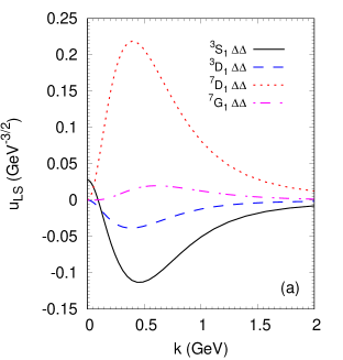
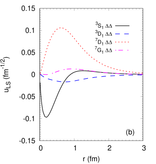
Figure 2: The wave functions of the $\Delta-\Delta$ system in momentum (a) and configuration (b) space.

The resulting c.m. momentum distribution is plotted in Fig. 3 by the solid line.

Figure 3: Momentum distribution of the struck $\Delta$ in the $\Delta-\Delta$ c.m. frame. Solid line: CCF model, Eq.(45). Long-dashed line: large-distance asymptotic solution, Eq.(48), obtained by setting $m_{\Delta}=m_{\Delta_{R}}=1.232$ GeV. Both lines are multiplied by an extra factor of 1/2 which is the isospin fraction of the $\Delta^{++}-\Delta^{-}$ component. The ordinary deuteron c.m. momentum distribution multiplied by a factor of $10^{-6}$ is shown by the short-dashed line.

The result of the coupled-channel model calculation is by far different from the simple large-distance asymptotic form

$$\phi_{\Delta-\Delta}(\mathbf{k})=\frac{(\kappa P_{\Delta-\Delta})^{1/2}/\pi}{\kappa^{2}+\mathbf{k}^{2}}~{},$$ (48)

where the range parameter is $\kappa=\sqrt{2\mu E_{b}}$ with the reduced mass $\mu=m_{\Delta}m_{\Delta_{R}}/(m_{\Delta}+m_{\Delta_{R}})$ and the binding energy $E_{b}=m_{\Delta}+m_{\Delta_{R}}-m_{d}$. Note that, owing to the large binding energy, the c.m. momentum distribution of the $\Delta-\Delta$ system is much harder than that of the ordinary deuteron.

The shapes of the $r$-space wave functions are similar to those of other potential models with $\Delta$ degrees-of-freedom (cf. Fig. 2 in ref. Haapakoski and Saarela (1974), Fig. 10 in ref. Niephaus et al. (1979), and Fig. 14 in ref. Wiringa et al. (1984)). In particular, the wave function of the dominating ${}^{7}D_{1}$ $\Delta-\Delta$ component is quite close to that of ref. Niephaus et al. (1979). There are some moderate differences for other components, e.g., in the CCF model the wave function of the ${}^{3}S_{1}$ $\Delta-\Delta$ component has a node at $r\simeq 0.9$ fm which is a feature of the particular coupled-channel model realization (see, however, ref. Dymarz and Khanna (1986) where a node in the ${}^{3}S_{1}$ $\Delta-\Delta$ component at $r\simeq 0.5$ fm has been reported too). Our feeling is that the differences in the momentum distribution Eq.(45) will be quite small between the various models. The main difference between the models and, thus, the major uncertainty concerns the total probability of the $\Delta-\Delta$ configuration, which varies between $\sim 0.3\%$ and $\sim 1\%$. In some sense the CCF model applied in this work represents the upper limit on the $\Delta-\Delta$ admixture in the deuteron.

4 Background processes

4.1 Pion charge exchange

The antiproton may annihilate with the neutron producing a $\pi^{-}\pi^{0}$ pair. The neutral pion may then experience inelastic CEX scattering on the proton producing a $\pi^{-}\Delta^{++}$ pair. This CEX background process is depicted in Fig. 4.

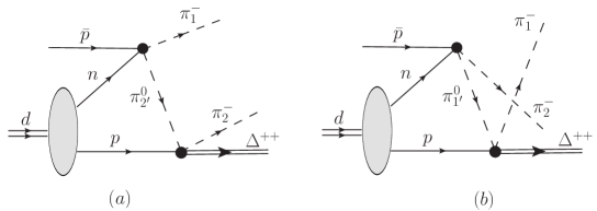
Figure 4: The background processes due to inelastic CEX of the neutral pion on the proton.

The amplitude of Fig. 4 can be calculated starting from the $S$-matrix.

However, a more economic way to derive it is to use the vertex function $\Gamma_{d\to np}(p_{d},p_{p})$ which is defined similar to Eq.(14):

$$\frac{i\Gamma_{d\to np}(p_{d},p_{p})}{p_{n}^{2}-m_{N}^{2}+i\epsilon}=\left(\frac{2E_{p}E_{d}}{E_{n}}\right)^{1/2}(2\pi)^{3/2}\phi(\mathbf{k})~{},$$ (49)

where $\phi(\mathbf{k})$ is the deuteron wave function in momentum space (spin indices are implicit), $\mathbf{k}=-\mathbf{p}_{p}+\mathbf{p}_{d}/2$, $E_{p}=\sqrt{\mathbf{p}_{p}^{2}+m_{N}^{2}}$, $E_{n}=E_{d}-E_{p}$. The invariant matrix element of Fig. 4a can be written as

$$iM_{\pi_{1}\pi_{2}\Delta_{R};\bar{p}d}^{(a)} = \int\frac{d^{4}p_{p}}{(2\pi)^{4}}iM_{\pi p}(p_{2},p_{\Delta};p_{2^{\prime}},p_{p})\frac{i}{p_{p}^{2}-m_{N}^{2}+i\epsilon}\frac{i}{p_{2^{\prime}}^{2}-m_{\pi}^{2}+i\epsilon}$$ (50)

$$\times iM_{\bar{p}n}(p_{1},p_{2^{\prime}};p_{\bar{p}},p_{n})\frac{i}{p_{n}^{2}-m_{N}^{2}+i\epsilon}\Gamma_{d\to np}(p_{d},p_{p})~{}.$$

The integration contour over $dp_{p}^{0}$ can be closed in the lower part of the complex plane where only the pole of the proton propagator at $p_{p}^{0}=E_{p}-i\epsilon$ contributes, such that

$$\int\frac{dp_{p}^{0}}{2\pi}\frac{i}{(p_{p}^{0})^{2}-E_{p}^{2}+i\epsilon}=\frac{1}{2E_{p}}~{}.$$ (51)

Hence we obtain

$$iM_{\pi_{1}\pi_{2}\Delta_{R};\bar{p}d}^{(a)} = \int\frac{d^{3}p_{p}}{(2\pi)^{3/2}}\left(\frac{E_{d}}{2E_{p}E_{n}}\right)^{1/2}iM_{\pi p}(p_{2},p_{\Delta};p_{2^{\prime}},p_{p})\frac{i}{p_{2^{\prime}}^{2}-m_{\pi}^{2}+i\epsilon}$$ (52)

$$\times iM_{\bar{p}n}(p_{1},p_{2^{\prime}};p_{\bar{p}},p_{n})\phi(\mathbf{k})~{}.$$

A kinematically interesting scenario for the “signal” process of antiproton annihilation on the $\Delta-\Delta$ state emerges in the case that both $t=(p_{1}-p_{\bar{p}})^{2}$ and $u=(p_{2}-p_{\bar{p}})^{2}$ (Fig. 1) are large, i.e. $t\sim u\sim-s/2$, since one has to resolve a short time interval of the deuteron existing in a $\Delta-\Delta$ state. Thus the $\bar{p}n\to\pi^{-}\pi^{0}$ amplitude is hard and can be factorized out in Eq.(52) by neglecting the neutron Fermi motion. Such regime corresponds to both pions having momenta with large positive $z$-components. Hence the momentum transfer $q=p_{p}-p_{\Delta}$ in the CEX process $\pi^{0}p\to\pi^{-}\Delta^{++}$ is small, $q^{2}\ll p_{2t}^{2}$. Under these assumptions the inverse propagator of the pion can be simplified:

$$p_{2^{\prime}}^{2}-m_{\pi}^{2}+i\epsilon=(p_{2}-q)^{2}-m_{\pi}^{2}+i\epsilon=2p_{2}^{z}\left(q^{z}-q^{0}\frac{E_{2}}{p_{2}^{z}}+\frac{\mathbf{p}_{2t}\mathbf{q}_{t}}{p_{2}^{z}}+\frac{q^{2}}{2p_{2}^{z}}+i\epsilon\right)$$

$$=2p_{2}^{z}(p_{p}^{z}+\Delta^{0}_{\pi}+i\epsilon)~{},$$ (53)

where

$$\Delta^{0}_{\pi}=-p_{\Delta}^{z}+(E_{\Delta}-m_{N})\frac{E_{2}}{p_{2}^{z}}+\frac{\mathbf{p}_{2t}(\mathbf{p}_{pt}-\mathbf{p}_{\Delta t})}{p_{2}^{z}}~{}.$$ (54)

In Eq.(54) we neglected the term $q^{2}/2p_{2}^{z}$ and the Fermi motion of the proton.

In the calculation of the pion CEX amplitude $M_{\pi p}(p_{2},p_{\Delta};p_{2^{\prime}},p_{p})$ we put the four-momentum $p_{2^{\prime}}$ of the intermediate pion on mass shell by setting $p_{p}^{z}=-\Delta^{0}_{\pi}$ for fixed proton transverse momentum $\mathbf{p}_{pt}$. After this setting the pion CEX amplitude becomes independent of the longitudinal momentum of the proton. This allows us to separate the integral over $dp_{p}^{z}$ in Eq.(52) with the inverse pion propagator of Eq.(53):

$$I_{z}=\int dp_{p}^{z}\frac{\phi(-\mathbf{p}_{p})}{p_{p}^{z}+\Delta^{0}_{\pi}+i\epsilon}~{},$$ (55)

as given in the deuteron rest frame. The deuteron wave function in momentum space can be expressed as follows (cf. Frankfurt et al. (1997)):

$$\phi(\mathbf{k})=\frac{1}{\sqrt{4\pi}}\left(u(k)+\frac{w(k)}{\sqrt{8}}S(\mathbf{k})\right)\chi^{M}$$ (56)

with the spin tensor operator

$$S(\mathbf{k})=\frac{3(\boldsymbol{\sigma}_{p}\mathbf{k})(\boldsymbol{\sigma}_{n}\mathbf{k})}{k^{2}}-\boldsymbol{\sigma}_{p}\boldsymbol{\sigma}_{n}~{},$$ (57)

and $\chi^{M}$ being the eigenfunction of the spin = 1 state with spin projection $M=0,\pm 1$. We will apply the analytical parameterization of the S- and D-wave components in the spirit of the Paris Lacombe et al. (1981) model, however, with the values of parameters adjusted according to the CCF model Haidenbauer et al. (1993)

$$u(k)=\sum_{j}\frac{c_{j}}{k^{2}+m_{j}^{2}}~{},~{}~{}~{}w(k)=\sum_{j}\frac{d_{j}}{k^{2}+m_{j}^{2}}~{},$$ (58)

with additional conditions $\sum_{j}c_{j}=0$ and $\sum_{j}d_{j}=\sum_{j}d_{j}/m_{j}^{2}=\sum_{j}d_{j}m_{j}^{2}=0$. These conditions guarantee the decrease of both wave functions $\propto 1/k^{4}$ at large $k$ and $w(k)\propto k^{2}$ at small $k$. The latter guarantees the absence of a pole at $k=0$ in the product $w(k)S(\mathbf{k})$.

The integration contour over $dp_{p}^{z}$ in Eq.(55) can be closed in the upper part of the complex plane where only the poles of the wave function at $p_{p}^{z}=im_{jt},m_{jt}=\sqrt{m_{j}^{2}+p_{pt}^{2}}$ contribute. This leads to the following expression for the longitudinal momentum integral:

$$I_{z}=\frac{1}{\sqrt{4\pi}}\sum_{j}\frac{\pi}{m_{jt}(\Delta^{0}_{\pi}+im_{jt})}\phi_{j}^{M}(-\mathbf{p}_{p})~{},$$ (59)

where

$$\phi_{j}^{M}(-\mathbf{p}_{p})=\left(c_{j}+\frac{d_{j}}{\sqrt{8}}S(-\mathbf{p}_{p})\right)\chi^{M}$$ (60)

with $\mathbf{p}_{p}=(\mathbf{p}_{pt},im_{jt})$. Using Eq.(59), after some algebra Eq.(52) can finally be transformed to the following expression:

$$M_{\pi_{1}\pi_{2}\Delta_{R};\bar{p}d}^{(a)} = -\frac{m_{d}^{1/2}M_{\bar{p}n}(p_{1},p_{\bar{p}}+p_{n}-p_{1};p_{\bar{p}},p_{n})}{16\pi m_{N}p_{2}^{z}}$$ (61)

$$\times\int d^{2}p_{pt}M_{\pi p}(p_{2},p_{\Delta};p_{2}+p_{\Delta}-p_{p},p_{p})\sum_{j}\frac{\phi_{j}^{M}(-\mathbf{p}_{pt},-im_{jt})}{m_{jt}(\Delta^{0}_{\pi}+im_{jt})}~{},$$

where $p_{n}=(m_{N},0)$ and $p_{p}=(\sqrt{m_{N}^{2}+p_{pt}^{2}+(\Delta^{0}_{\pi})^{2}},\mathbf{p}_{pt},-\Delta^{0}_{\pi})$ are the neutron and proton four-momenta in the elementary matrix elements. Note that the summation over spin indices of intermediate proton and neutron is implicitly assumed in Eq.(61).

4.2 Three-pion annihilation

Fig. 5 shows another possible background channel due to the two-step process $\bar{p}n\to\pi^{-}\pi^{-}\pi^{+},~{}\pi^{+}p\to\Delta^{++}$.

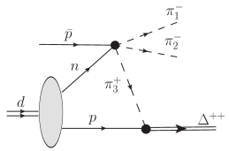
Figure 5: The background process initiated by antiproton annihilation on the neutron into three pions.

Similar to Eq.(52), the invariant matrix element of Fig. 5 can be expressed as

$$iM_{\pi_{1}\pi_{2}\Delta_{R};\bar{p}d}^{(3\pi)} = \int\frac{d^{3}p_{p}}{(2\pi)^{3/2}}\left(\frac{E_{d}}{2E_{p}E_{n}}\right)^{1/2}iM_{\pi p}(p_{\Delta};p_{3},p_{p})\frac{i}{p_{3}^{2}-m_{\pi}^{2}+i\epsilon}$$ (62)

$$\times iM_{\bar{p}n}(p_{1},p_{2},p_{3};p_{\bar{p}},p_{n})\phi(\mathbf{k})~{},$$

where the intermediate proton is put on mass shell, i.e. $p_{p}^{0}=E_{p}=\sqrt{\mathbf{p}_{p}^{2}+m_{N}^{2}}$, $p_{3}=p_{\Delta}-p_{p}$, $E_{n}=E_{d}-E_{p}$, and $\mathbf{k}=-\mathbf{p}_{p}+\mathbf{p}_{d}/2$.

Since all three particles in the $\pi N\Delta$ vertex have small momenta, the simplification of the pion propagator in Eq.(62) by neglecting proton Fermi motion in the spirit of Eq.(53) is generally impossible. Thus, we simplified Eq.(62) by only replacing proton and neutron energies in the denominator by the nucleon mass. The resulting expression in the deuteron rest frame is

$$M_{\pi_{1}\pi_{2}\Delta_{R};\bar{p}d}^{(3\pi)}=-\frac{m_{d}^{1/2}}{4\pi^{3/2}m_{N}}\int d^{2}p_{pt}\int\limits_{-\infty}^{+\infty}dp_{p}^{z}\frac{M_{\pi p}(p_{\Delta};p_{3},p_{p})M_{\bar{p}n}(p_{1},p_{2},p_{3};p_{\bar{p}},p_{n})\phi(-\mathbf{p}_{p})}{p_{3}^{2}-m_{\pi}^{2}+i\epsilon}~{}.$$ (63)

At fixed proton transverse momentum $\mathbf{p}_{pt}$, the pion propagator may have up to two poles at $p_{p}^{z}=\Delta_{1}$ and $p_{p}^{z}=\Delta_{2}$ with $\Delta_{1}\leq\Delta_{2}$. The poles are given by the zeros of the function

$$F(\mathbf{p}_{p})=p_{3}^{2}-m_{\pi}^{2}=(p_{\Delta}-p_{p})^{2}-m_{\pi}^{2}=m_{\Delta}^{2}+m_{N}^{2}-m_{\pi}^{2}-2E_{\Delta}E_{p}+2\mathbf{p}_{\Delta}\mathbf{p}_{p}~{}.$$ (64)

The calculation of the poles $\Delta_{1,2}$ is described in Appendix B. In order to avoid numerical problems related to the poles, we added a small artificial width to the pion. Thus, we replaced in Eq.(63) $\epsilon\to m_{\pi}\Gamma_{\pi}^{\rm art}$ with $\Gamma_{\pi}^{\rm art}\sim 10$ MeV. This allows to compute the three-dimensional integral over the proton momentum in the usual way. To achieve a smooth dependence of the matrix element on the momentum of the $\Delta$, the numerical integration on the proton transverse momentum has been performed separately in the subregions with and without pion poles, while the integration over $dp_{p}^{z}$ has been performed separately in the intervals $p_{p}^{z}<\Delta_{1}$, $\Delta_{1}<p_{p}^{z}<\Delta_{2}$ and $\Delta_{2}<p_{p}^{z}$. The moderate influence of the choice of the artificial pion width on the results is displayed in Fig.10 below.

One note is in order here. For simplicity, we perform the background calculations using the NR description of the deuteron. Since the ordinary deuteron wave function in momentum space is quite narrow (cf. Fig. 3) the NR approximation should be indeed reasonable in evaluating momentum space integrals like in Eqs.(61),(62), provided that the elementary amplitudes do not strongly grow in certain regions of momentum space. For example, in the case of pion inelastic CEX, the $\pi^{0}p\to\pi^{-}\Delta^{++}$ amplitude drops quickly with transverse momentum transfer and, thus, the integration over proton transverse momentum in Eq.(61) is unproblematic. However, the $\bar{p}n\to\pi^{-}\pi^{-}\pi^{+}$ amplitude $M_{\bar{p}n}(s^{\prime})$ extracted from the fit to the available experimental data (see Appendix C4) strongly grows with decreasing $s^{\prime}=(p_{\bar{p}}+p_{d}-p_{p})^{2}$. This makes the integral in Eq.(62) sensitive to the lower limit of $p_{p}^{z}$. Hence, in the spirit of the LC approach, we have restricted the longitudinal proton momentum integral by the condition $(E_{p}-p_{p}^{z})/m_{d}<1$.

5 Numerical results

The differential cross section of the background processes is expressed by Eq.(15) where one has to replace $M^{(0)}$ by $M^{(a)}+M^{(b)}$ for the pion CEX background (see Eq.(61) and the same equation with interchange $p_{1}\leftrightarrow p_{2}$ for $M^{(b)}$) or by $M^{(3\pi)}$ (see Eq.(63) for the three-pion annihilation background. Interference between signal and background processes is neglected. The calculation of the differential cross section $E_{\Delta}d^{4}\sigma/d^{3}p_{\Delta}dt$ for the background is numerically exhaustive, since it requires integration over pion azimuthal angle. Thus we have calculated the following quantity:

$$E_{\Delta}\frac{d^{5}\sigma}{d^{3}p_{\Delta}d\Omega_{\pi}}=\frac{\overline{|M_{\pi_{1}\pi_{2}\Delta;\bar{p}d}|^{2}}p_{1}^{2}}{32(2\pi)^{5}p_{\rm lab}m_{d}\kappa}~{},$$ (65)

where $\Omega_{\pi}$ is the solid angle defining the direction of the momentum $\mathbf{p}_{1}$ in the deuteron rest frame, $\kappa=|p_{1}E_{2}+(p_{1}-\tilde{\mathbf{p}}\cdot\mathbf{p}_{1}/p_{1})E_{1}|$, $\tilde{\mathbf{p}}=\mathbf{p}_{\bar{p}}-\mathbf{p}_{\Delta}$. In Eq.(65), $\overline{|M_{\pi_{1}\pi_{2}\Delta;\bar{p}d}|^{2}}$ should be replaced by the corresponding background or signal expression. For the signal, Eq.(17) is applied in the case of the NR description, while in the case of the LC description we have

$$\overline{|M^{(0)}_{\pi_{1}\pi_{2}\Delta;\bar{p}d}|^{2}}=\frac{2(m_{\Delta}^{2}+\bm{k}^{2})^{1/2}m_{d}}{(m_{d}-m_{\Delta})(2-\alpha)^{2}}(2\pi)^{3}|\phi_{\Delta-\Delta}(\bm{k})|^{2}\overline{|M_{\pi_{1}\pi_{2};\bar{p}\Delta_{S}}|^{2}}~{}.$$ (66)

All signal cross sections shown on the figures below include an extra factor of 1/2 which is the isospin fraction of the $\Delta^{-}-\Delta^{++}$ component.

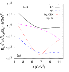
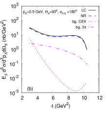
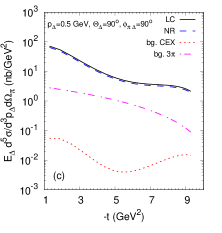
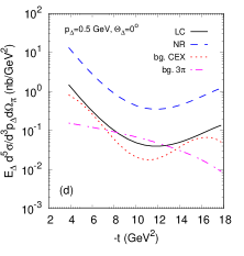
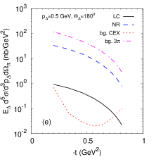
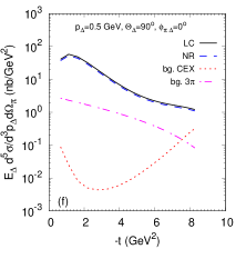
Figure 6: Differential cross section of the reaction $\bar{p}d\to\pi^{-}\pi^{-}\Delta^{++}$ at $p_{\rm lab}=10$ GeV/c as a function of the Mandelstam $t$, which is defined as the four-momentum transfer squared between one of the outgoing pions (1^st pion) and the antiproton (Eq.(28)). The solid, dashed, dotted, and dot-dashed lines correspond to the LC signal, NR signal, CEX background, and $3\pi$ background, respectively. Different panels display the results for the different values of the momentum $p_{\Delta}$ and the polar angle $\Theta_{\Delta}$ of the $\Delta$-isobar and of the relative azimuthal angle $\phi_{\pi\Delta}=\phi_{\pi}-\phi_{\Delta}$ between 1^st pion and $\Delta$. All quantities refer to the deuteron rest frame. The residual $\Delta^{++}$ is assumed to be on the mass shell.

Fig. 6 shows the differential $\bar{p}d\to\pi^{-}\pi^{-}\Delta^{++}$ cross sections calculated at 10 GeV/c beam momentum. The cross sections are plotted in the $t$-interval where both pions have $z$-components of their momenta larger than 1 GeV/c. On one hand, this condition is needed in order to ensure the “softness” of the pion CEX (otherwise our calculation becomes inapplicable). On the other hand, the most interesting case of hard $\bar{p}\Delta^{-}\to\pi^{-}\pi^{-}$ interaction – i.e. when $\Theta_{c.m.}\simeq 90\degree$ and both pions have momenta with $z$-components close to $p_{\rm lab}/2$ – is fully covered. We have considered the representative cases of the $\Delta$ at rest and of the $\Delta$ at 0.5 GeV/c momentum, emitted at polar angles $\Theta_{\Delta}=0\degree,90\degree$ and $180\degree$. In the case of $\Theta_{\Delta}=90\degree$ the cross section also depends on the azimuthal angle between $\pi$ and $\Delta$.

At zero momentum of the residual $\Delta$-resonance, the LC calculation produces much larger signal cross section than the NR calculation does. This can be traced back to the struck $\Delta$ momentum distribution in the $\Delta-\Delta$ c.m. frame (Fig. 3). In the NR calculation, the momentum $k$ of the struck $\Delta$ is zero, while in the LC calculation $k^{z}=0.4$ GeV/c corresponding to $\alpha=1.3$ for the residual $\Delta$ at rest. When the residual $\Delta$ moves transversely to the beam direction with momentum 0.5 GeV/c, the difference between LC and NR calculations is practically invisible. If the residual $\Delta$ moves in positive or negative $z$ direction with 0.5 GeV/c momentum, then the intrinsic momentum is $k^{z}=-0.14$ GeV/c or $3.77$ GeV/c, respectively, i.e. in regions where the struck $\Delta$ momentum distribution is strongly suppressed, and thus the LC calculation predicts much smaller signal cross section as compared to the NR calculation.

The characteristic shape of the $\Delta-\Delta$ momentum distribution (Fig. 3) is certainly of primary interest. One expects that it should be visible in the $\alpha$-distributions of the residual $\Delta$:

$$\alpha\beta\frac{d^{5}\sigma}{d\alpha d\beta d\phi_{\pi\Delta}p_{\Delta t}dp_{\Delta t}dp_{\Delta}^{2}}=\frac{\overline{|M_{\pi_{1}\pi_{2}\Delta;\bar{p}d}|^{2}}p_{1t}{\cal A}(p_{\Delta}^{2})}{16(2\pi)^{4}p_{\rm lab}m_{d}\kappa_{t}}~{},$$ (67)

where

$$\beta=\frac{2(E_{1}+p_{1}^{z})}{E_{\bar{p}}+m_{d}-E_{\Delta}+p_{\rm lab}-p_{\Delta}^{z}}$$ (68)

is the LC momentum fraction of one of the outgoing pions (“1^st pion”), and $\phi_{\pi\Delta}=\phi_{\pi}-\phi_{\Delta}$ is the relative azimuthal angle between the 1^st pion and the $\Delta$. The quantity

$$\kappa_{t}=2\left|p_{1t}\frac{E_{2}+p_{2}^{z}}{E_{1}+p_{1}^{z}}+p_{1t}+\frac{\mathbf{p}_{\Delta t}\cdot\mathbf{p}_{1t}}{p_{1t}}\right|$$ (69)

originates from expressing the phase space volume of the outgoing particles in terms of the LC momentum fractions and transverse momenta.

To take into account the possible off-shellness of the residual $\Delta$ we have also introduced in Eq.(67) the spectral function of the $\Delta$-resonance

$${\cal A}(p_{\Delta}^{2})=\frac{\sqrt{p_{\Delta}^{2}}\Gamma_{\Delta}/\pi}{(p_{\Delta}^{2}-m_{\Delta}^{2})^{2}+m_{\Delta}^{2}\Gamma_{\Delta}^{2}}~{},$$ (70)

normalized as

$$\int\limits_{(m_{\pi}+m_{N})^{2}}^{+\infty}{\cal A}(M^{2})dM^{2}=1~{}.$$ (71)

The off-shell background matrix elements are obtained in the usual way, i.e. by the replacements $m_{\Delta}\to\sqrt{p_{\Delta}^{2}}$. The expressions Eqs.(17),(66) for the moduli squared of the signal matrix elements and the relation Eq.(41) between the LC momentum fraction $\alpha$ and the internal momentum $\bm{k}$ are not modified due to the $\Delta^{++}$ off-shellness. In the numerical results below we have set the residual $\Delta^{++}$ on its mass shell.

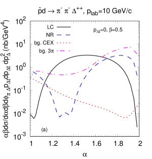
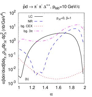
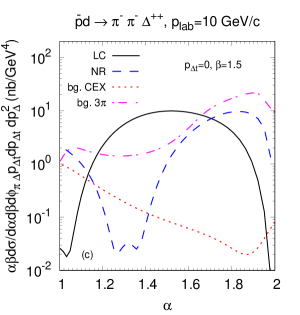
Figure 7: Differential cross section of the reaction $\bar{p}d\to\pi^{-}\pi^{-}\Delta^{++}$ at $p_{\rm lab}=10$ GeV/c as a function of the LC momentum fraction $\alpha$ of the residual $\Delta$ (Eq.(31)). The $\Delta$ transverse momentum is fixed to zero. The LC momentum fraction of the 1^st pion $\beta=0.5$ (a), $\beta=1$ (b) and $\beta=1.5$ (c). Notations for lines are the same as in Fig. 6.

Fig. 7 displays $\alpha$ distributions of the residual $\Delta$ at zero transverse momentum for $\beta=0.5,1$ and 1.5 for beam momentum $p_{\rm lab}=10$ GeV/c. Indeed, the shape of the $\alpha$ dependence of the signal cross section reflects the shape of the momentum dependence of the $\Delta-\Delta$ configuration. The latter has a maximum at $k=0.41$ GeV/c. In the case of $p_{\Delta t}=0$ this maximum is reached at $\alpha=1.80$ and $0.95$ (NR), or at $\alpha=1.32$ and $0.68$ (LC). Thus, due to the presence of the internal-momentum-dependent denominator in Eq.(41) the strength of the $\alpha$-distribution is shifted to smaller values of $\alpha$ (i.e. larger positive $p_{\Delta}^{z}$) in the case of LC calculation as compared to the NR one. Therefore, due to relativistic effects, the signal should be clearly visible at intermediate values of $\alpha$ because the background quickly decreases towards small $\alpha$. For $\beta=1.5$ the signal is more pronounced. This can be understood by using the approximate relation $\beta=1+\cos(\Theta_{c.m.})$. Thus, $\beta=1$ corresponds to $\Theta_{c.m.}=90\degree$ while $\beta=1.5$ corresponds to $\Theta_{c.m.}=60\degree$. In the latter case, as shown in Fig. 18 of Appendix C2, the elementary $\bar{p}\Delta^{-}\to\pi^{-}\pi^{-}$ differential cross section grows more slowly with decreasing $s^{\prime}$ at small $s^{\prime}$. (In order to avoid misunderstanding, we would like to point out that $s$ in the abscissa of Fig. 18 has the meaning of $s^{\prime}$ in Eq.(38).) As a result, the distortion of the $\alpha$ dependence of the signal due to the elementary $\bar{p}\Delta^{-}\to\pi^{-}\pi^{-}$ differential cross section growing towards $\alpha\to 2$ is less pronounced for $\beta=1.5$ than for $\beta=1$. Hence, we set $\beta=1.5$ as the default case.

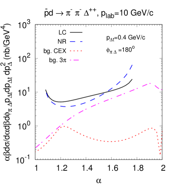
Figure 8: Same as in Fig. 7c but for $\Delta$ transverse momentum of 0.4 GeV/c. The polar angle between the 1^st pion and the residual $\Delta$ is $\phi_{\pi\Delta}=180\degree$. The range of $\alpha$ within which the signal calculations are shown is restricted by the kinematic region where the struck $\Delta$ is time-like.

At finite transverse momentum of the residual $\Delta$, the range of $\alpha$ where the struck $\Delta$ is still time-like becomes narrower. This is demonstrated in Fig. 8. At the limiting values of $\alpha$ the signal cross section diverges because the density matrix of a spin-3/2 particle (the numerator in Eq.(109)) becomes singular for $m_{\Delta}\to 0$. In other words, our calculation becomes unreliable for far-offshell struck $\Delta$. Below we focus on the kinematics with $p_{\Delta t}=0$.

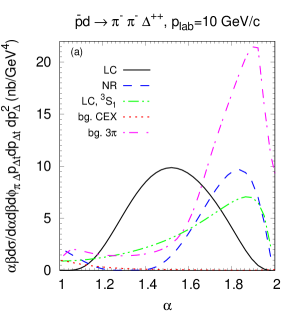
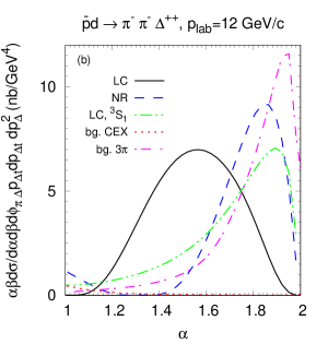
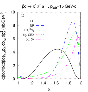
Figure 9: Differential cross section of the reaction $\bar{p}d\to\pi^{-}\pi^{-}\Delta^{++}$ vs $\alpha$ of the residual $\Delta$ for $p_{\rm lab}=10$ GeV/c (a) 12 GeV/c (b) and 15 GeV/c (c). Calculations are done with $p_{\Delta t}=0,\beta=1.5$. The dot-dot-dashed (green) line shows the LC signal calculated with the large-distance asymptotic form of the $\Delta-\Delta$ wave function, Eq.(48). The notations for other lines are the same as in Fig. 6.

Fig. 9 compares the $\alpha$ distributions at beam momenta $p_{\rm lab}=10,12$ and 15 GeV/c on the linear scale. Both signal and background cross sections slightly decrease with increasing $p_{\rm lab}$. However, the background decreases faster and becomes smoother at higher beam momenta. Hence, the peak in the signal cross section becomes more pronounced with increasing $p_{\rm lab}$. We also observe a strong influence of the underlying model for the $\Delta-\Delta$ wave function on the results: the LC calculation with the ${}^{3}S_{1}$ wave function produces an $\alpha$ distribution enhanced at larger $\alpha$ values. This is related to the larger high-momentum tail of the ${}^{3}S_{1}$ wave function, as seen from Fig. 3. The NR $\Delta-\Delta$ wave function – as compared to the LC one – leads to the signal $\alpha$ distribution shifted to larger $\alpha$ values, but its shape is still clearly distinguishable from the background.

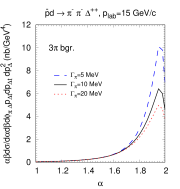
Figure 10: The three-pion annihilation background cross section as a function of $\alpha$ of the residual $\Delta$ for $p_{\rm lab}=15$ GeV/c at the kinematic condition $p_{\Delta t}=0$, $\beta=1.5$. The curves show the calculations with different choice of the artificial pion width as indicated.

As discussed in sec. 4.2, in the calculation of the three-pion background we had to introduce a finite value for the width of the intermediate $\pi^{+}$. Fig. 10 displays the influence of the choice of the pion width in our calculations. The height of the peak close to $\alpha=2$ depends on the choice of the pion width. However, the background in the range $\alpha<1.7$ is stable against variation of $\Gamma_{\pi}$.

We have performed a Monte-Carlo sampling of events in the three-body phase space of outgoing $\pi_{1},\pi_{2},\Delta$ according to the probability

$$dP\propto\overline{|M_{\pi_{1}\pi_{2}\Delta;\bar{p}d}|^{2}}d\Phi_{3}(p_{\bar{p}}+p_{d};p_{1},p_{2},p_{\Delta}){\cal A}(p_{\Delta}^{2})dp_{\Delta}^{2}~{},$$ (72)

where

$$d\Phi_{3}(p_{\bar{p}}+p_{d};p_{1},p_{2},p_{\Delta})=\delta^{(4)}(p_{1}+p_{2}+p_{\Delta}-p_{\bar{p}}-p_{d})\frac{d^{3}p_{\Delta}}{(2\pi)^{3}2E_{\Delta}}\frac{d^{3}p_{1}}{(2\pi)^{3}2E_{1}}\frac{d^{3}p_{2}}{(2\pi)^{3}2E_{2}}$$ (73)

is the three-body phase space volume element.

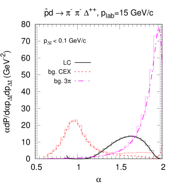
Figure 11: Histograms: probability distributions of the residual $\Delta^{++}$ in $\alpha$ at $p_{\rm lab}=15$ GeV/c in the kinematics with $p_{\Delta}^{2}=m_{\Delta}^{2}$; $p_{\Delta t}<0.1$ GeV/c; $\beta=1.4\div 1.6$; $p_{1}^{z},p_{2}^{z}>1$ GeV/c. Smooth lines: the analytical results of Fig. 9c multiplied by constant factors for appropriate normalization.

Fig. 11 shows the $\alpha$ distributions of simulated $\bar{p}d\to\pi^{-}\pi^{-}\Delta^{++}$ signal and background events for small transverse momentum of the residual $\Delta^{++}$. As we see, the sampled and analytical distributions practically coincide. Some deviation of the CEX background from the analytical result is due to its strong sensitivity to the transverse momentum of $\Delta$ at $\alpha\simeq 2$. (In the simulations we included the cut $p_{\Delta t}<1.9$ GeV/c for the CEX background). Note that the absolute values of the differential cross section are not accessible from Fig. 11 since the sampled distributions are normalized to unity after integration over $\alpha$ and $p_{\Delta t}$.

6 Summary and conclusions

We have theoretically studied the effect of the $\Delta^{-}-\Delta^{++}$ configuration of the deuteron on the differential cross sections of the exclusive reaction $\bar{p}d\to\pi^{-}\pi^{-}\Delta^{++}$. For the analysis we used the ordinary deuteron wave functions and the wave functions of the $\Delta-\Delta$ configuration according to the CCF model of ref. Haidenbauer et al. (1993). The signal cross section is proportional to the wave function squared of the $\Delta-\Delta$ configuration in momentum space and the matrix element squared of the $\bar{p}\Delta^{-}\to\pi^{-}\pi^{-}$ process. The latter has been calculated within the $N,\Delta$ exchange model. Two types of possible background sources due to the following two-step processes have been considered: (i) $\bar{p}n\to\pi^{-}\pi^{0}$, $\pi^{0}p\to\pi^{-}\Delta^{++}$ and (ii) $\bar{p}n\to\pi^{-}\pi^{-}\pi^{+}$, $\pi^{+}p\to\Delta^{++}$. The discussion was focused on kinematics with large momentum transfer between $\bar{p}$ and both $\pi^{-}$ mesons.

We have found that the pion CEX background (i) is important for forward production of $\Delta^{++}$ (cf. Fig. 6d). In this case the $\Delta^{++}$ may experience large longitudinal momentum transfer from the scattered pion. In other situations the CEX background is strongly suppressed relative to the three-pion annihilation background (ii). The latter background grows strongly for backward $\Delta^{++}$, because in this case the c.m. energy of the colliding $\bar{p}n$ system is small which leads to a large $\bar{p}n\to\pi^{-}\pi^{-}\pi^{+}$ amplitude.

Owing to the large binding of the $\Delta-\Delta$ configuration in the deuteron, the momentum distribution becomes significantly harder than in the ordinary deuteron. This leads to important relativistic corrections which have been taken into account in this work within the LC theory. Moreover, the coupled channel models of the deuteron with strong tensor interaction predict the dominance of the ${}^{7}D_{1}$ $\Delta-\Delta$ state which produces a pronounced maximum at about 0.5 GeV/c c.m. momentum. We have demonstrated that the combination of LC and coupled channel effects leads to a specific shape of the $\alpha$ distribution of the residual $\Delta^{++}$ peaking at $\alpha\simeq 1.5\div 1.6$ for zero transverse momentum, which manifests the maximum in the $\Delta-\Delta$ c.m. momentum distribution. This behaviour of the signal cross section is clearly distinguishable from the three-pion annihilation background smoothly increasing with $\alpha$. We have also found that there is a broad kinematic range of residual $\Delta^{++}$ ($\alpha=1.2\div 1.7,~{}p_{\Delta t}<0.4$ GeV/c), where the one-step signal process dominates over the two-step background processes. Even if the $\Delta-\Delta$ probability would be reduced by a factor of five down to $\sim 0.3\%$ – the $\alpha$-distribution of the $\Delta$ at low transverse momentum (Fig. 9c) would still allow to see the contribution of the $\bar{p}$ annihilation on the $\Delta-\Delta$ component. These findings can be used not only to test the presence of the $\Delta-\Delta$ configuration in the deuteron, but also to explore its c.m. momentum distribution.

On the basis of our model we have developed a Monte-Carlo event generator which can be applied for detailed feasibility studies with the PANDA detector system. The results of these studies will be published elsewhere. Note that a complementary test of the ${}^{7}D_{1}$ $\Delta-\Delta$ state dominance would be possible with a polarized deuteron target at PANDA.

Finally, we note that the previous experimental analyses quoted in sec. 1 do not take into account the LC wave function, and thus their conclusions on limits to the probability of a $\Delta-\Delta$ configuration need to be taken with caution.

Appendix A Relation between the LC and NR wave functions of the $\Delta-\Delta$ system

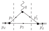
Figure 12: Lowest order contribution to the absorption amplitude of a photon on the deuteron. $q$, $p_{d}$ and $p_{d}^{\prime}$ are the four-momenta of the photon, initial and final deuteron, respectively. $p_{1}$, $p_{2}$ and $p_{1}^{\prime}$ are the four-momenta of the intermediate $\Delta$’s. Time axis is from left to right.

Consider the electromagnetic formfactor of the deuteron viewed as a $\Delta-\Delta$ state, Fig. 12. In the kinematics of high-energy $ed$ scattering in the c.m. frame of colliding particles the four-momentum transfer from electron to deuteron can be written as follows (see equation on p. 225 of ref. Frankfurt and Strikman (1981), note opposite direction of $z$-axis):

$$q=\left(\frac{2\nu+q^{2}}{4P},\bm{q}_{t},\frac{2\nu-q^{2}}{4P}\right)~{},$$ (74)

where $P\to+\infty$ is the electron momentum directed along the $z$-axis (correspondingly, $p_{d}^{z}=-P$) and $\nu=p_{d}q$. At very large $P$ the four-momentum transfer becomes purely transverse. This allows to consider only the graph of Fig. 12, since other graphs contain pair production and disappear for $q^{z}=0$. The matrix element of Fig. 12 can be calculated within the non-covariant perturbation theory rules Weinberg (1966) which give the following expression:

$$M(\bm{q}_{t})=-\Gamma_{d\to\Delta\Delta}^{2}\int\frac{d^{3}p_{2}}{(2\pi)^{3}}\frac{M_{\gamma^{*}}(q;p_{1})}{2E_{\bm{p}_{2}}2E_{\bm{p}_{1}}2E_{\bm{p}_{1}^{\prime}}}\frac{1}{p_{d}^{0}-E_{\bm{p}_{2}}-E_{\bm{p}_{1}}+i\epsilon}\frac{1}{p_{d}^{0\prime}-E_{\bm{p}_{2}}-E_{\bm{p}_{1}^{\prime}}+i\epsilon}~{},$$ (75)

where $E_{\bm{p}_{i}}=\sqrt{m_{\Delta}^{2}+\bm{p}_{i}^{2}},i=1,2,1^{\prime}$ are the energies of the intermediate $\Delta$’s with three-momenta $\bm{p}_{1}=\bm{p}_{d}-\bm{p}_{2}$, $\bm{p}_{1}^{\prime}=\bm{q}+\bm{p}_{d}-\bm{p}_{2}$, and $M_{\gamma^{*}}(q;p_{1})$ is the invariant matrix element of the electromagnetic transition, $\gamma\Delta\to\Delta$ (the spin indices are implicit). For simplicity, a constant vertex factor $\Gamma_{d\to\Delta\Delta}$ is assumed. Introducing the ratios

$$\alpha_{i}=\frac{-2p_{i}^{z}}{P},~{}~{}~{}i=1,2,1^{\prime}~{},$$ (76)

the particle energies can be expressed as

$$E_{\bm{p}_{i}}=\frac{|\alpha_{i}|P}{2}+\frac{m_{i}^{2}+\bm{p}_{it}^{2}}{|\alpha_{i}|P}+O(1/P^{3})~{}.$$ (77)

Using the relations $\alpha_{1}+\alpha_{2}=\alpha_{1^{\prime}}+\alpha_{2}=2$, $\bm{p}_{1t}=\bm{p}_{1^{\prime}t}-\bm{q}_{t}=-\bm{p}_{2t}$, which follow from three-momentum conservation at the vertices, and the relation

$$\frac{d^{3}p_{2}}{E_{\bm{p}_{2}}}=\frac{d\alpha_{2}d^{2}p_{2t}}{\alpha_{2}}~{},$$ (78)

the matrix element Eq.(75) can be expressed as follows:

$$M(\bm{q}_{t})=-\Gamma_{d\to\Delta\Delta}^{2}\int\limits_{0}^{2}\frac{d\alpha_{2}}{2\alpha_{2}(2-\alpha_{2})^{2}}\int\frac{d^{2}p_{2t}}{(2\pi)^{3}}\frac{2}{m_{d}^{2}-M_{1,2}^{2}}\frac{2M_{\gamma^{*}}(\bm{q}_{t};\alpha_{1},\bm{p}_{1t})}{m_{d}^{2}-M_{1^{\prime},2}^{2}}~{},$$ (79)

where

$$M_{1,2}^{2} = \frac{4(m_{\Delta}^{2}+p_{2t}^{2})}{\alpha_{2}(2-\alpha_{2})},$$ (80)

$$M_{1^{\prime},2}^{2} = \frac{2(m_{\Delta}^{2}+p_{2t}^{2})}{\alpha_{2}}+\frac{2(m_{\Delta}^{2}+(\bm{q}_{t}-\bm{p}_{2t})^{2})}{2-\alpha_{2}}-q_{t}^{2}~{}.$$ (81)

Using the internal three-momenta $\bm{k}$ and $\bm{k}^{\prime}$ defined as

$$\alpha_{2} = 1+\frac{k^{z}}{\sqrt{m_{\Delta}^{2}+\bm{k}^{2}}}~{},~{}~{}~{}\bm{k}_{t}=-\bm{p}_{2t}~{},$$ (82)

$$\alpha_{2} = 1+\frac{k^{\prime z}}{\sqrt{m_{\Delta}^{2}+\bm{k}^{\prime 2}}}~{},~{}~{}~{}\bm{k}^{\prime}_{t}=\bm{k}_{t}+\frac{1}{2}\alpha_{2}\bm{q}_{t}~{},$$ (83)

and the relation

$$\frac{d\alpha_{2}d^{2}p_{2t}}{\alpha_{2}(2-\alpha_{2})}=\frac{d^{3}k}{\sqrt{m_{\Delta}^{2}+\bm{k}^{2}}}$$ (84)

one can express Eq.(79) in the form

$$M(\bm{q}_{t})=-\Gamma_{d\to\Delta\Delta}^{2}\int\frac{d^{3}k}{(2\pi)^{3}\sqrt{m_{\Delta}^{2}+\bm{k}^{2}}(2-\alpha_{2})}\frac{1}{m_{d}^{2}-M_{1,2}^{2}}\frac{2M_{\gamma^{*}}(\bm{q}_{t};\alpha_{1},\bm{k}_{t})}{m_{d}^{2}-M_{1^{\prime},2}^{2}}~{},$$ (85)

with $M_{1,2}^{2}=4(m_{\Delta}^{2}+\bm{k}^{2})$ and $M_{1^{\prime},2}^{2}=4(m_{\Delta}^{2}+\bm{k}^{\prime 2})$. We can now introduce the LC wave function of the $\Delta-\Delta$ state defined according to ref. Frankfurt and Strikman (1981) (see sec. 2.3.1 of ref. Frankfurt and Strikman (1981), the vertex function $\chi$ is replaced by $i\Gamma_{d\to\Delta\Delta}$ in our notation):

$$\psi_{\Delta-\Delta}(k)=\frac{i\Gamma_{d\to\Delta\Delta}}{M_{1,2}^{2}-m_{d}^{2}}~{}.$$ (86)

Then Eq.(85) can be rewritten in the form

$$M(\bm{q}_{t})=\int\frac{d^{3}k}{(2\pi)^{3}\sqrt{m_{\Delta}^{2}+\bm{k}^{2}}(2-\alpha_{2})}\psi_{\Delta-\Delta}(k)\psi_{\Delta-\Delta}(k^{\prime})2M_{\gamma^{*}}(\bm{q}_{t};2-\alpha_{2},\bm{k}_{t})~{}.$$ (87)

Note that in the chosen frame the matrix element (87) is the only contribution to the Lorentz-invariant matrix element calculated within the Feynman rules because the graphs with pair production disappear in this frame.

On the other hand, we can calculate the photo-absorption amplitude in the NR approximation. In this case we choose the frame, where both the initial and the final deuteron move slowly, $|\bm{p}_{d}|,|\bm{p}_{d}^{\prime}|\ll m_{d}$, but the electron is fast. We start from the $S$-matrix element corresponding to Fig. 12 (spin indices are suppressed for brevity):

$$S_{\rm NR} = \int d^{3}r_{1}\int d^{3}r_{2}\int d^{3}r_{1}^{\prime}\int d^{3}r_{2}^{\prime}\phi_{\Delta-\Delta,f}^{*}(\bm{r}_{1}^{\prime},\bm{r}_{2}^{\prime})\phi_{\Delta-\Delta,i}(\bm{r}_{1},\bm{r}_{2})$$ (88)

$$\times\frac{1}{V^{2}}\int\frac{Vd^{3}p_{1}}{(2\pi)^{3}}\int\frac{Vd^{3}p_{2}}{(2\pi)^{3}}\int\frac{Vd^{3}p_{1}^{\prime}}{(2\pi)^{3}}e^{-i\bm{p}_{1}\bm{r}_{1}-i\bm{p}_{2}\bm{r}_{2}+i\bm{p}_{1}^{\prime}\bm{r}_{1}^{\prime}+i\bm{p}_{2}\bm{r}_{2}^{\prime}}S_{\gamma^{*}}(q;p_{1})~{},$$

where

$$S_{\gamma^{*}}(q;p_{1})=\frac{(2\pi)^{4}\delta^{(4)}(p_{1}^{\prime}-p_{1}-q)}{(2E_{1}V2E_{1}^{\prime}V2q^{0}V)^{1/2}}\,iM_{\gamma^{*}}(q;p_{1})~{}.$$ (89)

Here $E_{1}=p_{d}^{0}-E_{\bm{p}_{2}}$ and $E_{1}^{\prime}=p_{d}^{\prime 0}-E_{\bm{p}_{2}}$ are the energies of the 1^st $\Delta$ before and after $\gamma^{*}$-absorption (the 2^nd $\Delta$ is put on the mass shell).

By integrating out the c.m. motion (similar to Eq.(7) of sec. 2) we obtain the usual transition $S$-matrix in a factorized form:

$$S_{\rm NR}=\frac{(2\pi)^{4}\delta^{(4)}(p_{d}^{\prime}-p_{d}-q)}{(2p_{d}^{0}V2p_{d}^{\prime 0}V2q^{0}V)^{1/2}}\,iM_{\rm NR}~{},$$ (90)

where the invariant matrix element is

$$M_{\rm NR}=\int d^{3}p_{2}\left(\frac{p_{d}^{0}p_{d}^{\prime 0}}{E_{1}E_{1}^{\prime}}\right)^{1/2}\phi_{\Delta-\Delta}^{*}\left(\frac{\bm{p}_{d}^{\prime}}{2}-\bm{p}_{2}\right)\phi_{\Delta-\Delta}\left(\frac{\bm{p}_{d}}{2}-\bm{p}_{2}\right)M_{\gamma^{*}}(q;p_{d}-p_{2})~{}.$$ (91)

Note that one can obtain Eq.(91) also by treating the graph Fig. 12 as a Feynman diagram and then using the relation (14).

It follows from Eq.(2.22) of ref. Frankfurt and Strikman (1981) (where one should replace the nucleon mass by the $\Delta$ mass) that the function $\psi_{\Delta-\Delta}(k)/(m_{\Delta}^{2}+\bm{k}^{2})^{1/4}$ satisfies the non-relativistic Schrödinger equation for the $\Delta-\Delta$ bound state with binding energy $2m_{\Delta}-m_{d}$ and the potential corresponding to the kernel of the Bethe-Salpeter-type equation. Thus the function $\psi_{\Delta-\Delta}(k)/(m_{\Delta}^{2}+\bm{k}^{2})^{1/4}$ should be proportional to the NR wave function $\phi_{\Delta-\Delta}(k)$. The proportionality factor can be obtained by taking the limit $q=0$ (forward $ed$ scattering) and assuming a very narrow wave function $\phi_{\Delta-\Delta}(k)$ peaking at $k=0$. In this case the LC and NR expressions, i.e. Eqs.(87) and (91) with $\bm{p}_{d}=\bm{p}_{d}^{\prime}=0$, should coincide. This leads to the following relation

$$\frac{2\psi_{\Delta-\Delta}^{2}(k)}{(2\pi)^{3}(m_{\Delta}^{2}+\bm{k}^{2})^{1/2}}=\frac{m_{d}}{m_{d}-m_{\Delta}}\phi_{\Delta-\Delta}^{2}(k)~{}.$$ (92)

Appendix B Poles of the pion propagator

To determine the poles of the pion propagator in the three-pion annihilation background (see Fig. 5) for fixed values of the proton transverse momentum, let us consider the $\pi^{+}p\to\Delta^{++}$ transition in the frame where the $\Delta$ has a momentum with a large negative $z$-component. In that frame, the four-momenta of the $\Delta$, pion and proton are, respectively,

$$p_{\Delta} = (P+\frac{m_{\Delta t}^{2}}{2P},\mathbf{p}_{\Delta t},-P)~{},$$ (93)

$$p_{\pi} = (P\alpha_{\pi}+\frac{m_{\pi t}^{2}}{2P\alpha_{\pi}},\mathbf{p}_{\pi t},-P\alpha_{\pi})~{},$$ (94)

$$p_{p} = (P\alpha_{p}+\frac{m_{pt}^{2}}{2P\alpha_{p}},\mathbf{p}_{pt},-P\alpha_{p})~{},$$ (95)

where the transverse masses are $m_{\Delta t}=\sqrt{\mathbf{p}_{\Delta t}^{2}+m_{\Delta}^{2}}$, $m_{\pi t}=\sqrt{\mathbf{p}_{\pi t}^{2}+m_{\pi}^{2}}$ with $\mathbf{p}_{\pi t}=\mathbf{p}_{\Delta t}-\mathbf{p}_{pt}$, and $m_{pt}=\sqrt{\mathbf{p}_{pt}^{2}+m_{N}^{2}}$, and $P\to+\infty$. $\alpha_{\pi}$ and $\alpha_{p}$ are the longitudinal-boost-invariant momentum fractions of the $\Delta$ carried by the pion and proton, respectively. They satisfy the condition $\alpha_{\pi}+\alpha_{p}=1$. In the lab. frame the fractions can be expressed as

$$\alpha_{\pi}=\frac{E_{\pi}-p_{\pi}^{z}}{E_{\Delta}-p_{\Delta}^{z}}~{},~{}~{}~{}\alpha_{p}=\frac{E_{p}-p_{p}^{z}}{E_{\Delta}-p_{\Delta}^{z}}~{}.$$ (96)

Energy conservation can be expressed as

$$\frac{m_{\pi t}^{2}}{\alpha_{\pi}}+\frac{m_{pt}^{2}}{\alpha_{p}}=m_{\Delta t}^{2}~{}.$$ (97)

This equation can be easily solved with respect to $\alpha_{p}$:

$$\alpha_{p}=(A\pm\sqrt{A^{2}-B})/2~{},$$ (98)

where

$$A=\frac{m_{pt}^{2}+m_{\Delta t}^{2}-m_{\pi t}^{2}}{m_{\Delta t}^{2}}~{},~{}~{}~{}B=\frac{4m_{pt}^{2}}{m_{\Delta t}^{2}}~{}.$$ (99)

The fraction of the deuteron momentum carried by the proton is then

$$\tilde{\alpha}_{p}=\tilde{\alpha}_{\Delta}\alpha_{p}~{},$$ (100)

where in the deuteron rest frame

$$\tilde{\alpha}_{p}=\frac{E_{p}-p_{p}^{z}}{m_{d}/2}~{},~{}~{}~{}\tilde{\alpha}_{\Delta}=\frac{E_{\Delta}-p_{\Delta}^{z}}{m_{d}/2}~{}.$$ (101)

Thus the two poles of the pion propagator are given by

$$p_{p}^{z}=\Delta_{1,2}=\frac{m_{pt}^{2}}{m_{d}\tilde{\alpha}_{p}}-\frac{m_{d}\tilde{\alpha}_{p}}{4}~{}.$$ (102)

The $\Delta_{1}$ ($\Delta_{2}$) is obtained by choosing $+$ ($-$) sign in Eq.(98).

Appendix C Elementary amplitudes

Appendix C1 $\bar{N}N\to\pi\pi$

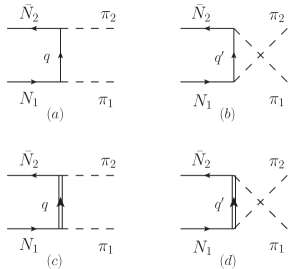
Figure 13: Feynman graphs included in the calculation of the $\bar{N}_{2}N_{1}\to\pi_{2}\pi_{1}$ amplitude. Graphs (a) and (b) contain the exchange of a nucleon. Graphs (c) and (d) contain the exchange of a $\Delta$-isobar. The four-momenta of the exchange particle are denoted as $q$ and $q^{\prime}$, respectively, in the $t$-channel (a,c) and $u$-channel (b,d) graphs, where $t=q^{2}$, $u=q^{\prime 2}$.

The amplitude of antinucleon-nucleon annihilation into two pions is described within the nucleon and $\Delta$ exchange model as displayed in Fig. 13. For the $\pi NN$ and $\pi N\Delta$ interactions we apply the following Lagrangians:

$${\cal L}_{\pi NN} = \frac{f_{\pi NN}}{m_{\pi}}\bar{\psi}\gamma^{\mu}\gamma^{5}\boldsymbol{\tau}\psi\partial_{\mu}\boldsymbol{\pi}~{},$$ (103)

$${\cal L}_{\pi N\Delta} = \frac{f_{\pi N\Delta}}{m_{\pi}}\bar{\psi}^{\mu}\boldsymbol{T}\psi\partial_{\mu}\boldsymbol{\pi}+h.c.~{},$$ (104)

where $f_{\pi NN}=1.008$, $f_{\pi N\Delta}=2.202$ Dmitriev et al. (1986). Here, $\boldsymbol{T}$ is the isospin transition $1/2\to 3/2$ operator (cf. ref. Brown and Weise (1975)):

$$\boldsymbol{T}_{\tau_{\Delta}\tau_{N}}=\sum_{l=0,\pm 1}<\frac{3}{2}\tau_{\Delta}|\frac{1}{2}\tau_{N};1l>\boldsymbol{t}^{(l)*}~{},$$ (105)

with $\boldsymbol{t}^{(0)}=(0,0,1),\boldsymbol{t}^{(\pm 1)}=\mp\frac{1}{\sqrt{2}}(1,\pm i,0)$ being the eigenvectors of $\hat{I}^{2}$ and $\hat{I}_{3}$ operators for $I=1$ in Cartesian basis. The invariant matrix elements of the graphs (a) and (c) are

$$M_{\bar{N}N}^{(a)} = \left(\frac{f_{\pi NN}F_{\pi NN}(t)}{m_{\pi}}\right)^{2}\frac{{\cal I}_{\bar{N}N}^{(a)}\sqrt{\Omega}}{t-m_{N}^{2}+i\epsilon}\bar{u}(-p_{2},-\lambda_{2})\not{k}_{2}(\not{q}-m_{N})\not{k}_{1}u(p_{1},\lambda_{1})~{},$$ (106)

$$M_{\bar{N}N}^{(c)} = -\left(\frac{f_{\pi N\Delta}F_{\pi N\Delta}(t,m_{\Delta}^{2})}{m_{\pi}}\right)^{2}\frac{{\cal I}_{\bar{N}N}^{(c)}\sqrt{\Omega}}{t-m_{\Delta}^{2}+i\epsilon}$$ (107)

$$\times\bar{u}(-p_{2},-\lambda_{2})(\not{q}+m_{\Delta})k_{2\mu}k_{1\nu}{\cal P}^{\mu\nu}(q)u(p_{1},\lambda_{1})~{},$$

where $p_{1},\lambda_{1}$ and $p_{2},\lambda_{2}$ are the four-momenta and spin projections of the nucleon and antinucleon, respectively, and $k_{1},k_{2}$ are the four-momenta of the pions. The Dirac spinors are normalized as $\bar{u}_{p_{1},\lambda_{1}}u_{p_{1},\lambda_{1}}=-\bar{u}_{-p_{2},-\lambda_{2}}u_{-p_{2},-\lambda_{2}}=2m_{N}$. In obtaining Eqs.(106),(107) we used the Dirac propagator of the nucleon

$$iG(q)=\frac{i(\not{q}+m_{N})}{q^{2}-m_{N}^{2}+i\epsilon}~{},$$ (108)

and the Rarita-Schwinger propagator of the $\Delta$-isobar

$$iG^{\mu\nu}(q)=\frac{-i(\not{q}+m_{\Delta})}{q^{2}-m_{\Delta}^{2}+i\epsilon}{\cal P}^{\mu\nu}(q)~{},$$ (109)

where

$${\cal P}^{\mu\nu}(q)=g^{\mu\nu}-\frac{\gamma^{\mu}\gamma^{\nu}}{3}-\frac{2q^{\mu}q^{\nu}}{3m_{\Delta}^{2}}+\frac{q^{\mu}\gamma^{\nu}-q^{\nu}\gamma^{\mu}}{3m_{\Delta}}~{}.$$ (110)

The isospin factors are expressed as

$${\cal I}_{\bar{N}N}^{(a)} = (-1)^{1/2+\tau_{2}}\sum_{\tau_{N}=\pm 1/2}(\boldsymbol{t}^{(l_{2})*}\cdot\boldsymbol{\tau})_{-\tau_{2},\tau_{N}}(\boldsymbol{t}^{(l_{1})*}\cdot\boldsymbol{\tau})_{\tau_{N},\tau_{1}}~{},$$ (111)

$${\cal I}_{\bar{N}N}^{(c)} = (-1)^{1/2+\tau_{2}}\sum_{\tau_{\Delta}=\pm 1/2,\pm 3/2}(\boldsymbol{t}^{(l_{2})*}\cdot\boldsymbol{T}^{\dagger})_{-\tau_{2},\tau_{\Delta}}(\boldsymbol{t}^{(l_{1})*}\cdot\boldsymbol{T})_{\tau_{\Delta},\tau_{1}}~{},$$ (112)

where $l_{1},l_{2}=0,\pm 1$ are the isospin projections of the pions, and $\tau_{1},\tau_{2}=\pm 1/2$ are the isospin projections of nucleon and antinucleon, respectively. The common factor $(-1)^{1/2+\tau_{2}}$ originates from the definition of the physical antineutron state as $|\bar{n}>=-|\bar{N},\tau=+1/2>$ as follows from the relation $\hat{G}|\bar{N},\tau>=-|N,\tau>$, where $\hat{G}=\exp(i\pi\hat{I}_{2})\hat{C}$ is the $G$-parity transformation operator Tabakin and Eisenstein (1985). For the $u$-channel graphs (b,d), the matrix elements are obtained by replacing $k_{1}\leftrightarrow k_{2}$, $q\to q^{\prime}$ and $t\to u$ in Eqs.(106),(107) and the isospin factors – by replacing $l_{1}\leftrightarrow l_{2}$ in Eqs.(111),(112). For the channels with incoming antiproton the values of isospin factors are listed in Table 1.

Table 1: Isospin factors in the nucleon and $\Delta$ exchange amplitudes of Fig. 13.

Channel	${\cal I}_{\bar{N}N}^{(a)}$	${\cal I}_{\bar{N}N}^{(b)}$	${\cal I}_{\bar{N}N}^{(c)}$	${\cal I}_{\bar{N}N}^{(d)}$
$\bar{p}p\to\pi^{-}\pi^{+}$	-2	0	-1/3	-1
$\bar{p}p\to\pi^{0}\pi^{0}$	1	1	2/3	2/3
$\bar{p}n\to\pi^{-}\pi^{0}$	$-\sqrt{2}$	$\sqrt{2}$	$\sqrt{2}/3$	$-\sqrt{2}/3$

To describe the finite size of the hadrons, we included formfactors in Eqs.(106),(107). Their choice is defined by the asymptotic scaling law Brodsky and Farrar (1973) at $s\to\infty,t/s={\rm const}$:

$$\frac{d\sigma}{dt}=\frac{f(t/s)}{s^{n}}~{},~{}~{}~{}n=\sum n_{i}-2~{},$$ (113)

where $n_{i}$ is the number of the constituents in the incoming and outgoing particles ($n_{B}=3,n_{M}=2$). Hence, $n=8$ for $\bar{N}N\to\pi\pi$. By counting the powers of $s$ (assuming $t\sim u\sim s$) one can deduce from the expression

$$\frac{d\sigma}{dt}=\frac{\overline{|M_{\bar{N}N}^{(a)}+M_{\bar{N}N}^{(b)}+M_{\bar{N}N}^{(c)}+M_{\bar{N}N}^{(d)}|^{2}}}{64\pi(s/4-m_{N}^{2})s}~{},$$ (114)

the powers of the vertex formfactors:

$$F_{\pi NN}(t) = \left(\frac{\Lambda_{\pi NN}^{2}-m_{N}^{2}}{\Lambda_{\pi NN}^{2}-t}\right)^{2}~{},$$ (115)

$$F_{\pi N\Delta}(t,M^{2}) = \left(\frac{\Lambda_{\pi N\Delta}^{2}-M^{2}}{\Lambda_{\pi N\Delta}^{2}-t}\right)^{5/2}~{}.$$ (116)

Finally, following ref. Sopkovich (1962) the attenuation factor $\sqrt{\Omega}$ is introduced in Eqs.(106),(107) to describe the initial-state interaction in the $\bar{N}N$ channel. For simplicity, we assume this factor to be energy- and angular-momentum-independent Larionov and Lenske (2017).

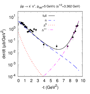
Figure 14: Differential cross section of the $\bar{p}p\to\pi^{-}\pi^{+}$ process at $p_{\rm lab}=5$ GeV/c. Solid line: full calculation. Dashed, dotted and dash-dotted lines display the separate contributions of neutron, $\Delta^{0}$ and $\Delta^{++}$ exchange, respectively. Experimental data are from ref. Eide et al. (1973).

The values of the cutoff parameters $\Lambda_{\pi NN}=2.0$ GeV and $\Lambda_{\pi N\Delta}=1.8$ GeV have been adjusted to describe the shape of the $t$-dependence of the differential cross section $d\sigma_{\bar{p}p\to\pi^{-}\pi^{+}}/dt$ at $p_{\rm lab}=5$ GeV/c. After this, the parameter $\Omega=0.008$ has been chosen to describe the absolute values of $d\sigma_{\bar{p}p\to\pi^{-}\pi^{+}}/dt$ close to $\Theta_{c.m.}=90\degree$ ($-t=4.7$ Gev²). This value of $\Omega$ is within the range of values from ref. Larionov and Lenske (2017), where meson-exchange models have been applied for the calculation of the $\bar{p}p\to\bar{\Lambda}\Lambda$ cross section.

Fig. 14 shows the comparison with experimental data for the fitted values of the parameters. At small $-t$ (forward c.m. angles) the main contribution is given by neutron exchange, while at large $-t$ (backward c.m. angles) the cross section is almost entirely due to $\Delta^{++}$ exchange. These features are in line with other calculations Van de Wiele and Ong (2010); Wang et al. (2017).

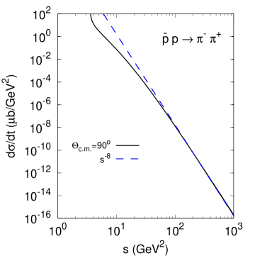
Figure 15: Solid line: differential cross section of the $\bar{p}p\to\pi^{-}\pi^{+}$ process calculated from Eq.(114) at $\Theta_{c.m.}=90\degree$ as a function of invariant $s$. Dashed line: large $s$ asymptote $\propto s^{-8}$.

In Fig. 15 we display the $s$ dependence of $d\sigma_{\bar{p}p\to\pi^{-}\pi^{+}}/dt$ at $-t=s/2-m_{N}^{2}-m_{\pi}^{2}$. The quark counting rule at large $s$ is reproduced exactly.

Appendix C2 $\bar{N}\Delta\to\pi\pi$

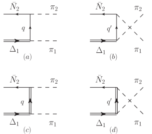
Figure 16: Same as Fig. 13, but for the $\bar{N}_{2}\Delta_{1}\to\pi_{2}\pi_{1}$ amplitude.

The Feynman graphs included in the nucleon-delta annihilation amplitude into two pions are shown in Fig. 16. The $\pi NN$ and $\pi N\Delta$ coupling Lagrangians were already explained in the previous subsection (see Eqs.(103),(104)). The $\pi\Delta\Delta$ coupling Lagrangian can be defined as follows (cf. ref. Matsuyama et al. (2007)):

$${\cal L}_{\pi\Delta\Delta}=\frac{f_{\pi\Delta\Delta}}{m_{\pi}}\bar{\psi}^{\nu}\gamma^{5}\gamma^{\mu}\boldsymbol{T}_{\Delta}\psi_{\nu}\partial_{\mu}\boldsymbol{\pi}~{},$$ (117)

where

$$(\boldsymbol{T}_{\Delta})_{\tau_{\Delta_{2}}\tau_{\Delta_{1}}}=\frac{\sqrt{15}}{2}\sum_{l=0,\pm 1}<\frac{3}{2}\tau_{\Delta_{2}}|\frac{3}{2}\tau_{\Delta_{1}};1l>\boldsymbol{t}^{(l)*}~{},$$ (118)

is the isospin operator for $I=3/2$. Within the SU(6) chiral constituent quark model the following relation holds Matsuyama et al. (2007):

$$f_{\pi\Delta\Delta}=\frac{6}{5}f_{\pi NN}~{}.$$ (119)

The invariant matrix elements of the $t$-channel graphs (a) and (c) of Fig. 16 are

$$M_{\bar{N}\Delta}^{(a)} = \frac{f_{\pi NN}F_{\pi NN}(t)f_{\pi N\Delta}F_{\pi N\Delta}(t,m_{N}^{2})}{m_{\pi}^{2}}\frac{{\cal I}_{\bar{N}\Delta}^{(a)}\sqrt{\Omega}}{t-m_{N}^{2}+i\epsilon}$$ (120)

$$\times\bar{u}(-p_{2},-\lambda_{2})\not{k}_{2}\gamma^{5}(\not{q}+m_{N})k_{1\mu}u^{\mu}(p_{1},\lambda_{1})~{},$$

$$M_{\bar{N}\Delta}^{(c)} = -\frac{f_{\pi N\Delta}F_{\pi N\Delta}(t,m_{\Delta}^{2})f_{\pi\Delta\Delta}F_{\pi\Delta\Delta}(t)}{m_{\pi}^{2}}\frac{{\cal I}_{\bar{N}\Delta}^{(c)}\sqrt{\Omega}}{t-m_{\Delta}^{2}+i\epsilon}$$ (121)

$$\times\bar{u}(-p_{2},-\lambda_{2})(\not{q}+m_{\Delta})k_{2}^{\mu}{\cal P}_{\mu\nu}(q)\gamma^{5}\not{k}_{1}u^{\nu}(p_{1},\lambda_{1})~{},$$

where the isospin factors are

$${\cal I}_{\bar{N}\Delta}^{(a)} = (-1)^{1/2+\tau_{2}}\sum_{\tau_{N}=\pm 1/2}(\boldsymbol{t}^{(l_{2})*}\cdot\boldsymbol{\tau})_{-\tau_{2},\tau_{N}}(\boldsymbol{t}^{(l_{1})*}\cdot\boldsymbol{T}^{\dagger})_{\tau_{N},\tau_{\Delta_{1}}}~{},$$ (122)

$${\cal I}_{\bar{N}\Delta}^{(c)} = (-1)^{1/2+\tau_{2}}\sum_{\tau_{\Delta}=\pm 1/2,\pm 3/2}(\boldsymbol{t}^{(l_{2})*}\cdot\boldsymbol{T}^{\dagger})_{-\tau_{2},\tau_{\Delta}}(\boldsymbol{t}^{(l_{1})*}\cdot\boldsymbol{T}_{\Delta})_{\tau_{\Delta},\tau_{\Delta_{1}}}~{}.$$ (123)

The $u$-channel matrix elements of the graphs (b) and (d) of Fig. 16 are obtained from Eqs.(120),(121) by the replacements $k_{1}\leftrightarrow k_{2}$, $q\to q^{\prime}$ and $t\to u$, and the corresponding isospin factors – by replacement $l_{1}\leftrightarrow l_{2}$ in Eqs.(122),(123). After some algebra we get the following values for the channel $\bar{p}\Delta^{-}\to\pi^{-}\pi^{-}$: ${\cal I}_{\bar{N}\Delta}^{(a)}={\cal I}_{\bar{N}\Delta}^{(b)}=\sqrt{2}$, ${\cal I}_{\bar{N}\Delta}^{(c)}={\cal I}_{\bar{N}\Delta}^{(d)}=1/\sqrt{2}$.

To get the high energy asymptotic behavior of Eq.(113) with $n=8$, the $\pi\Delta\Delta$ vertex formfactor should be taken in the form

$$F_{\pi\Delta\Delta}(t)=\left(\frac{\Lambda_{\pi\Delta\Delta}^{2}-m_{\Delta}^{2}}{\Lambda_{\pi\Delta\Delta}^{2}-t}\right)^{3}~{}.$$ (124)

The value of the cutoff $\Lambda_{\pi\Delta\Delta}$ is quite uncertain. However, we expect that it should not strongly deviate from $\Lambda_{\pi N\Delta}$ in the hard regime $-t\sim-u\sim s/2,s\to+\infty$. This is supported by the result of the previous subsection, that the cutoffs $\Lambda_{\pi N\Delta}$ and $\Lambda_{\pi NN}$ are also quite similar. Thus, to reduce the number of free parameters, we set $\Lambda_{\pi\Delta\Delta}=\Lambda_{\pi N\Delta}$.

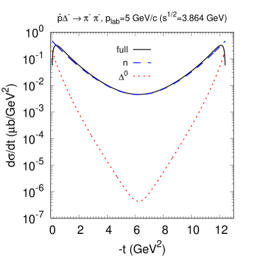
Figure 17: Differential cross section of the $\bar{p}\Delta^{-}\to\pi^{-}\pi^{-}$ process at $p_{\rm lab}=5$ GeV/c. Solid line: full calculation. Dashed and dotted lines display the separate contributions of neutron and $\Delta^{0}$ exchange, respectively.

Fig. 17 shows the $t$ dependence of the $\bar{p}\Delta^{-}\to\pi^{-}\pi^{-}$ differential cross section at 5 GeV/c beam momentum. (The cross section is symmetric with respect to replacement $t\leftrightarrow u$.) We see that $\Delta^{0}$ exchange is important at small $-t$, but becomes almost negligible at $\Theta_{c.m.}=90\degree$ (i.e. at $-t=(s-m_{N}^{2}-m_{\Delta}^{2})/2-m_{\pi}^{2}$).

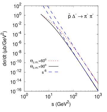
Figure 18: Differential cross section of the $\bar{p}\Delta^{-}\to\pi^{-}\pi^{-}$ process at $\Theta_{c.m.}=90\degree$ (solid line) and $60\degree$ (dotted line). The large-$s$ asymptotic behavior $\propto s^{-8}$ is shown for both cases by the dashed lines.

Fig. 18 displays the $s$ dependence of $d\sigma/dt$ at $\Theta_{c.m.}=90\degree$ and $60\degree$ for the $\bar{p}\Delta^{-}\to\pi^{-}\pi^{-}$ process. At large $s$, the quark counting rule is exactly respected.

Appendix C3 $\pi N\to\pi^{\prime}\Delta$ charge exchange

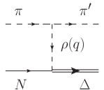
Figure 19: Feynman graph of the inelastic pion CEX amplitude $\pi N\to\pi^{\prime}\Delta$ due to $t$-channel $\rho$-meson exchange.

The amplitude of Fig. 19 has been evaluated with the $\rho\pi\pi$ interaction Lagrangian Serot and Walecka (1986)

$${\cal L}_{\rho\pi\pi}=g_{\rho\pi\pi}[\partial^{\mu}\boldsymbol{\pi}\times\boldsymbol{\pi}]\cdot\boldsymbol{\rho}_{\mu}~{},$$ (125)

where $g^{2}_{\rho\pi\pi}/4\pi=2.88$ (cf. ref. Van de Wiele and Ong (2010)) such that the $\rho$ decay width

$$\Gamma_{\rho\to\pi\pi}=\frac{g^{2}_{\rho\pi\pi}}{4\pi}\frac{m_{\rho}}{12}\left(1-\frac{4m_{\pi}^{2}}{m_{\rho}^{2}}\right)^{3/2}$$ (126)

is equal to the phenomenological value $0.150$ GeV at the pole mass $m_{\rho}=0.771$ GeV. The $\rho N\Delta$ interaction Lagrangian has been taken in the form with derivative coupling Shyam and Mosel (2003); Matsuyama et al. (2007):

$${\cal L}_{\rho N\Delta}=\frac{if_{\rho N\Delta}}{m_{\rho}}(\bar{\psi}^{\mu}\gamma^{\nu}\gamma^{5}\boldsymbol{T}\psi-\bar{\psi}\gamma^{\nu}\gamma^{5}\boldsymbol{T}^{\dagger}\psi^{\mu})(\partial_{\nu}\boldsymbol{\rho}_{\mu}-\partial_{\mu}\boldsymbol{\rho}_{\nu})~{}.$$ (127)

We will use the value of the coupling constant $f_{\rho N\Delta}=14.0$ which is about two times larger than in refs. Shyam and Mosel (2003); Matsuyama et al. (2007) but agrees with estimations in ref. Oset et al. (1982).

The invariant amplitude corresponding to Fig. 19 can be expressed as

$$M_{\pi N} = -i\frac{g_{\rho\pi\pi}f_{\rho N\Delta}}{m_{\rho}}\frac{{\cal I}_{\pi N}}{t-m_{\rho}^{2}+i\epsilon}(k+k^{\prime})^{\mu}\left(-g_{\mu\nu}+\frac{q_{\mu}q_{\nu}}{m_{\rho}^{2}}\right)$$ (128)

$$\times[-\bar{u}^{\nu}(p_{\Delta},\lambda_{\Delta})\not{q}\gamma^{5}u(p,\lambda)+\bar{u}^{\alpha}(p_{\Delta},\lambda_{\Delta})q_{\alpha}\gamma^{\nu}\gamma^{5}u(p,\lambda)]~{},$$

where $k$ and $k^{\prime}$ are the four-momenta of the incoming and outgoing pion, respectively, and $t=q^{2}$. The Rarita-Schwinger vector-spinors of the $\Delta$-resonance are normalized as $\bar{u}^{\mu}(p_{\Delta},\lambda_{\Delta})u_{\mu}(p_{\Delta},\lambda_{\Delta})=-2m_{\Delta}$. The isospin factor is

$${\cal I}_{\pi N}=\boldsymbol{T}_{\tau_{\Delta}\tau}\cdot[\boldsymbol{t}^{(l)}\times\boldsymbol{t}^{(l^{\prime})*}]~{},$$ (129)

where $\tau=\pm 1/2$ and $\tau_{\Delta}=\pm 1/2,\pm 3/2$ are the isospin projections of nucleon and $\Delta$, respectively, and $l,l^{\prime}=0,\pm 1$ are the isospin projections of the incoming and outgoing pion, respectively. For the relevant channel $\pi^{0}p\to\pi^{-}\Delta^{++}$ (and also for the channel $\pi^{+}p\to\pi^{0}\Delta^{++}$) we obtain ${\cal I}_{\pi N}=i$.

Small $-t$ scattering at high energies is well described within Regge theory, which approximates the exchange of a set of particles with the same internal quantum numbers (such as $B,I,S$ etc.) by the exchange of a Regge trajectory Collins (1977); Guidal et al. (1997). In particular, the $\rho$ meson trajectory includes the $a_{2}(1320)$, $\rho_{3}(1690)$, and $a_{4}(2040)$ states. The reggeization of the amplitude, Eq.(128), is reached by replacing

$$\frac{1}{t-m_{\rho}^{2}+i\epsilon}\to{\cal P}^{\rho}_{\rm Regge}=\left(\frac{s}{s_{0}}\right)^{\alpha_{\rho}(t)-1}\frac{\pi\alpha_{\rho}^{\prime}}{\sin(\pi\alpha_{\rho}(t))}\frac{-1+\exp(-i\pi\alpha_{\rho}(t))}{2}\frac{1}{\Gamma(\alpha_{\rho}(t))}~{},$$ (130)

where $s_{0}=1$ GeV², $\alpha_{\rho}(t)=\alpha_{\rho 0}+\alpha_{\rho}^{\prime}t$ with an intercept $\alpha_{\rho 0}$ and a slope $\alpha_{\rho}^{\prime}$ determined from the data on exclusive reactions assuming linearity of the $\rho$ meson trajectory and imposing the condition that $\alpha_{\rho}(m_{\rho}^{2})=1$.

We have calculated the differential cross section

$$\frac{d\sigma}{dt}=\frac{\overline{|M_{\pi N}|^{2}}}{64\pi(p_{\rm lab}m_{N})^{2}}~{},$$ (131)

of the $\pi^{+}p\to\pi^{0}\Delta^{++}$ process with different parameters of the $\rho$ Regge trajectory. As shown in Fig. 20, the intercept $\alpha_{\rho 0}=0.49$ and slope $\alpha_{\rho}^{\prime}=0.94$ GeV^-2 produce a quite reasonable description of available experimental data at small $-t$. Thus, these parameters are used in the calculations of the CEX background (sec. 4.1).

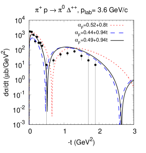
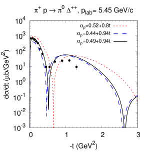
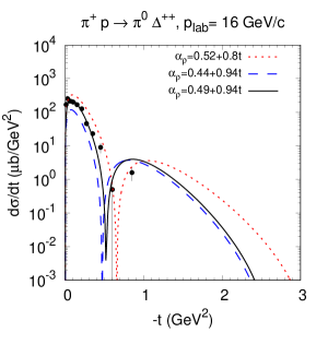
Figure 20: Differential cross section of the $\pi^{+}p\to\pi^{0}\Delta^{++}$ CEX process. Different curves represent calculations with different parameters of the $\rho$ meson Regge trajectory as indicated. Experimental data at 3.6 GeV/c, 5.45 GeV/c, and 16 GeV/c are from ref. Macnaughton et al. (1977), Bloodworth et al. (1974), and Honecker et al. (1977), respectively.

Appendix C4 $\bar{N}N\to\pi\pi\pi$

For the three-pion annihilation amplitude we assume an $s$-dependent invariant matrix element extracted from the fit of the $\bar{p}n\to\pi^{-}\pi^{-}\pi^{+}$ cross section, see Fig. 21, by the function

$$\sigma_{\bar{p}n\to\pi^{-}\pi^{-}\pi^{+}}=11.8\exp(-1.35\,p_{\rm lab})~{},$$ (132)

where $p_{lab}$ is in GeV/c and the cross section in mb.

Figure 21: Fit to the experimental data of ref. Eastman et al. (1973) on the $\bar{p}n\to\pi^{-}\pi^{-}\pi^{+}$ cross section by the exponential function given in Eq.(132).

The invariant matrix element can be estimated as

$$M_{\bar{p}n}(s)=\left(\frac{4I_{\bar{p}n}\sigma_{\bar{p}n\to\pi^{-}\pi^{-}\pi^{+}}}{(2\pi)^{4}\Phi_{3}(s)}\right)^{1/2}~{},$$ (133)

where $I_{\bar{p}n}=\sqrt{(s/4-m_{N}^{2})s}$ is the Möller flux factor and $\Phi_{3}(s)$ is the 3-body phase space integral (cf. PDG review Patrignani et al. (2016)).

Appendix C5 $\pi N\to\Delta$

The $\pi N\Delta$ interaction is described by the standard $P$-wave coupling Lagrangian of Eq.(104). The invariant matrix element of the $\pi^{+}p\to\Delta^{++}$ transition (see Fig. 5) is

$$iM_{\pi p}(p_{\Delta};p_{3},p_{p})=\frac{f_{\pi N\Delta}F_{\pi N\Delta}(p_{3})}{m_{\pi}}p_{3\mu}\bar{u}^{\mu}(p_{\Delta},\lambda_{\Delta})u(p_{p},\lambda_{p})~{}.$$ (134)

The formfactor is chosen in the monopole form

$$F_{\pi N\Delta}(q)=\frac{\Lambda^{2}-m_{\pi}^{2}}{\Lambda^{2}+\boldsymbol{q}^{2}}~{},$$ (135)

with $\Lambda=1.2$ GeV Dymarz and Khanna (1990). Note that the formfactors of Eq.(116) and Eq.(135) differ since they are applied in different regimes: the former is valid in the hard while the latter is valid in the soft regime.