Analysis of a chemo-repulsion model with nonlinear production: The continuous problem and unconditionally energy stable fully discrete schemes

Abstract

We consider the following repulsive-productive chemotaxis model: Let $p\in(1,2)$, find $u\geq 0$, the cell density, and $v\geq 0$, the chemical concentration, satisfying

$$\left\{\begin{array}[c]{lll}\partial_{t}u-\Delta u-\nabla\cdot(u\nabla v)=0\ \ \mbox{ in}\ \Omega,\ t>0,\\ \partial_{t}v-\Delta v+v=u^{p}\ \ \mbox{ in}\ \Omega,\ t>0,\end{array}\right.$$ (1)

in a bounded domain $\Omega\subseteq\mathbb{R}^{d}$, $d=2,3$. By using a regularization technique, we prove the existence of solutions for problem (1). Moreover, we propose three fully discrete Finite Element (FE) nonlinear approximations of problem (1), where the first one is defined in the variables $(u,v)$, and the second and third ones introduce ${\boldsymbol{\sigma}}=\nabla v$ as auxiliary variable. We prove some unconditional properties such as mass-conservation, energy-stability and solvability of the schemes. Finally, we compare the behavior of these schemes throughout several numerical simulations and give some conclusions.

2010 Mathematics Subject Classification. 35K51, 35Q92, 65M12, 65M60, 92C17.

Keywords: Chemorepulsion-production model, finite element approximation, unconditional energy-stability, nonlinear production.

1 Introduction

Chemotaxis is the biological process of the movement of living organisms in response to a chemical stimulus, which can be given towards a higher (chemo-attraction) or lower (chemo-repulsion) concentration of a chemical substance. At the same time, the presence of living organisms can produce or consume chemical substance. A repulsive-productive chemotaxis model can be given by the following parabolic PDE’s system:

$$\left\{\begin{array}[c]{lll}\partial_{t}u-\Delta u=\nabla\cdot(u\nabla v)\quad\mbox{ in}\ \Omega,\ t>0,\\ \partial_{t}v-\Delta v+v=f(u)\quad\mbox{ in}\ \Omega,\ t>0,\end{array}\right.$$

where $\Omega\subseteq\mathbb{R}^{d}$, $d=2,3$, is a bounded domain with boundary $\partial\Omega$. The unknowns for this model are $u(\textit{{x}},t)\geq 0$, the cell density, and $v(\textit{{x}},t)\geq 0$, the chemical concentration. Moreover, $f(u)\geq 0$ (if $u\geq 0$) is the production term. In this paper, we consider the particular case in which $f(u)=u^{p}$, with $1<p<2$, and then we focus on the following initial-boundary value problem:

$$\left\{\begin{array}[c]{lll}\partial_{t}u-\Delta u=\nabla\cdot(u\nabla v)\ \ \mbox{ in}\ \Omega,\ t>0,\\ \partial_{t}v-\Delta v+v=u^{p}\ \ \mbox{ in}\ \ \Omega,\ t>0,\\ \displaystyle\frac{\partial u}{\partial\mathbf{n}}=\frac{\partial v}{\partial\mathbf{n}}=0\ \ \mbox{on}\ \partial\Omega,\ t>0,\\ u(\textit{{x}},0)=u_{0}(\textit{{x}})>0,\ v(\textit{{x}},0)=v_{0}(\textit{{x}})>0\ \ \mbox{in}\ \Omega.\end{array}\right.$$ (2)

In the case of linear ($p=1$) and quadratic ($p=2$) production terms, the problem (2) is well-posed (see [7, 13] respectively) in the following sense: there exist global in time weak solutions (based on an energy inequality) and, for $2D$ domains, there exists a unique global in time strong solution. However, as far as we know, there are not works studying problem (2) with production $u^{p}$, with $1<p<2$.
Problem (2) is conservative in $u$, because the total mass $\int_{\Omega}u(\cdot,t)$ remains constant in time, as we can check integrating equation (2)₁ in $\Omega$,

$$\frac{d}{dt}\left(\int_{\Omega}u(\cdot,t)\right)=0,\ \ \mbox{ i.e. }\ \int_{\Omega}u(\cdot,t)=\int_{\Omega}u_{0}:=m_{0},\ \ \forall t>0.$$ (3)

The first aim of this work is to study the existence of weak-strong solutions for problem (2) (in the sense of Definition 3.1 below), satisfying in particular the energy inequality (9) below. The second aim of this work is to design numerical methods for model (2) conserving, at the discrete level, the mass-conservation and energy-stability properties of the continuous model (see (3) and (9), respectively).

There are only a few works about numerical analysis for chemotaxis models. For instance, for the Keller-Segel system (i.e. with chemo-attraction and linear production), in [9] Filbet proved the existence of discrete solutions and the convergence of a finite volume scheme. Saito, in [20, 21], studied error estimates for a conservative Finite Element (FE) approximation. In [8], some error estimates are proved for a fully discrete discontinuous FE method, and a mixed FE approximation is studied in [18].

Energy stable numerical schemes have also been studied in the chemotaxis framework. An energy-stable finite volume scheme for a Keller-Segel model with an additional cross-diffusion term has been studied in [6]. In [13, 14], unconditionally energy stable time-discrete numerical schemes and fully discrete FE schemes for a chemo-repulsion model with quadratic production have been analyzed. In [15], the authors studied unconditionally energy stable fully discrete FE schemes for a chemo-repulsion model with linear production. However, as far as we know, for the chemo-repulsion model with production term $u^{p}$ (2) there are not works studying energy-stable numerical schemes.

The outline of this paper is as follows: In Section 2, we give the notation and some preliminary results that will be used throughout the paper. In Section 3, we prove the existence of weak-strong solutions of model (2) (in the sense of Definition 3.1 below) by using a regularization technique. In Section 4, we propose three fully discrete FE nonlinear approximations of problem (2), where the first one is defined in the variables $(u,v)$, and the second and third ones introduce ${\boldsymbol{\sigma}}=\nabla v$ as an auxiliary variable. We prove some unconditional properties such as mass-conservation, energy-stability and solvability of the schemes. In Section 5, we compare the behavior of the schemes throughout several numerical simulations; and in Section 6, the main conclusions obtained in this paper are sumarized.

2 Notation and preliminary results

We recall some functional spaces which will be used throughout this paper. We will consider the usual Lebesgue spaces $L^{q}(\Omega),$ $1\leq q\leq\infty,$ with norm $\|\cdot\|_{L^{q}}$. In particular, the $L^{2}(\Omega)$-norm will be denoted by $\|\cdot\|_{0}$. From now on, $(\cdot,\cdot)$ will denote the standard $L^{2}$-inner product over $\Omega$. We also consider the usual Sobolev spaces $W^{m,p}(\Omega)=\{u\in L^{p}(\Omega):\|\partial^{\alpha}u\|_{L^{p}}<+\infty,\ \forall|\alpha|\leq m\}$, for a multi-index $\alpha$ and $m\in\mathbb{N}$, with norm denoted by $\|\cdot\|_{W^{m,p}}$. In the case when $p=2$, we denote $H^{m}(\Omega):=W^{m,2}(\Omega)$, with respective norm $\|\cdot\|_{m}$. Moreover, we denote by

$$W^{m,p}_{\mathbf{n}}(\Omega):=\left\{u\in W^{m,p}(\Omega):\frac{\partial{u}}{\partial\mathbf{n}}=0\ \mbox{ on }\ \partial\Omega\right\},$$

$${\boldsymbol{H}}^{1}_{\sigma}(\Omega):=\{\mathbf{\boldsymbol{\sigma}}\in{\boldsymbol{H}}^{1}(\Omega):\mathbf{\boldsymbol{\sigma}}\cdot\mathbf{n}=0\mbox{ on }\partial\Omega\},$$

and we will use the following equivalent norms in $H^{1}(\Omega)$ and ${{\boldsymbol{H}}}_{\sigma}^{1}(\Omega)$, respectively (see [19] and [2, Corollary 3.5], respectively):

$$\|u\|_{1}^{2}=\|\nabla u\|_{0}^{2}+\left(\int_{\Omega}u\right)^{2},\ \ \forall u\in H^{1}(\Omega),$$

$$\|{\boldsymbol{\sigma}}\|_{1}^{2}=\|{\boldsymbol{\sigma}}\|_{0}^{2}+\|\mbox{rot }{\boldsymbol{\sigma}}\|_{0}^{2}+\|\nabla\cdot{\boldsymbol{\sigma}}\|_{0}^{2},\ \ \forall{\boldsymbol{\sigma}}\in{\boldsymbol{H}}^{1}_{\sigma}(\Omega),$$ (4)

where rot ${\boldsymbol{\sigma}}$ denotes the well-known rotational operator (also called curl) which is scalar for 2D domains and vectorial for 3D ones. In particular, (4) implies that, for all $\boldsymbol{\sigma}=\nabla v\in{\boldsymbol{H}}^{1}_{\sigma}(\Omega)$,

$$\|\nabla v\|_{1}^{2}=\|\nabla v\|_{0}^{2}+\|\Delta v\|_{0}^{2}.$$ (5)

If $Z$ is a general Banach space, its topological dual space will be denoted by $Z^{\prime}$. Moreover, the letters $C,K$ will denote different positive constants which may change from line to line.
We will use the following results:

Theorem 2.1.

([10]) Let $1<q<+\infty$ and suppose that $f\in L^{q}(0,T;L^{q}(\Omega))$, $u_{0}\in\widehat{W}^{2-\frac{2}{q},q}(\Omega)$, where

$$\widehat{W}^{2-\frac{2}{q},q}(\Omega)\quad:=\quad\left\{\begin{array}[]{l}{W}^{2-\frac{2}{q},q}(\Omega)\ \ \mbox{ if }\ \ q<3,\\ {W}_{\mathbf{n}}^{2-\frac{2}{q},q}(\Omega)\ \ \mbox{ if }\ \ q>3.\\ \end{array}\right.$$

Then, the problem

$$\left\{\begin{array}[c]{lll}\partial_{t}u-\Delta u=f\ \ \mbox{ in}\ \Omega,\ t>0,\\ \displaystyle\frac{\partial u}{\partial\mathbf{n}}=0\ \ \mbox{on}\ \partial\Omega,\ t>0,\\ u({\textit{{x}}},0)=u_{0}({\textit{{x}}})\ \ \mbox{in}\ \Omega,\end{array}\right.$$

admits a unique solution $u$ in the class

$$u\in L^{q}(0,T;W^{2,q}(\Omega))\cap C([0,T];\widehat{W}^{2-\frac{2}{q},q}(\Omega)),\ \ \partial_{t}u\in L^{q}(0,T;L^{q}(\Omega)).$$

Moreover, there exists a positive constant $C=C(q,\Omega,T)$ such that

$$\|u\|_{C([0,T];\widehat{W}^{2-\frac{2}{q},q}(\Omega))}+\|\partial_{t}u\|_{L^{q}(0,T;L^{q}(\Omega))}+\|u\|_{L^{q}(0,T;W^{2,q}(\Omega))}\leq C(\|f\|_{L^{q}(0,T;L^{q}(\Omega))}+\|u_{0}\|_{\widehat{W}^{2-\frac{2}{q},q}(\Omega)}).$$

Proposition 2.2.

([1]) Let $X$ be a Banach space, $\Omega\subseteq X$ an open subset, $U\subseteq\Omega$ a nonempty convex subset and $J:\Omega\rightarrow\mathbb{R}$ a functional. Suppose that $J$ is $G-$differentiable in $\Omega$. Then, $J$ is convex over $U$ if and only if the following relation holds

$$J(x_{1})-J(x_{2})\leq\delta J(x_{1},x_{1}-x_{2}),\ \forall x_{1},x_{2}\in U,\ x_{1}\neq x_{2}.$$ (6)

Finally, we will use the following result to get large time estimates [16]:

Lemma 2.3.

Assume that $\delta,\beta,k>0$ and $d^{n}\geq 0$ satisfy

$$(1+\delta k)d^{n+1}\leq d^{n}+k\beta,\ \ \ \forall n\geq 0.$$

Then, for any $n_{0}\geq 0$,

$$d^{n}\leq(1+\delta k)^{-(n-n_{0})}d^{n_{0}}+\delta^{-1}\beta,\ \ \ \forall n\geq n_{0}.$$

3 Analysis of the continuous model

In this section, we will prove the existence of weak-strong solutions of problem (2) in the sense of the following definition.

Definition 3.1.

(Weak-strong solutions of (2)) Let $1<p<2$. Given $(u_{0},v_{0})\in L^{p}(\Omega)\times H^{1}(\Omega)$ with $u_{0}\geq 0$, $v_{0}\geq 0$ a.e. in $\Omega$, a pair $(u,v)$ is called weak-strong solution of problem (2) in $(0,+\infty)$, if $u\geq 0$, $v\geq 0$ a.e. in $(0,+\infty)\times\Omega$,

$$\begin{array}[]{ccc}u\in L^{\infty}(0,+\infty;L^{p}(\Omega))\cap L^{\frac{5p}{p+3}}(0,T;W^{1,\frac{5p}{p+3}}(\Omega)),\ \ \forall T>0,\\ v\in L^{\infty}(0,+\infty;H^{1}(\Omega))\cap L^{2}(0,T;H^{2}(\Omega)),\ \ \forall T>0,\\ \partial_{t}u\in L^{\frac{10p}{3p+6}}(0,T;W^{1,\frac{10p}{7p-6}}(\Omega)^{\prime}),\ \ \partial_{t}v\in L^{\frac{5}{3}}(0,T;L^{\frac{5}{3}}(\Omega)),\ \ \forall T>0,\end{array}$$

the following variational formulation for the $u$-equation holds

$$\int_{0}^{T}\langle\partial_{t}u,\bar{u}\rangle+\int_{0}^{T}(\nabla u,\nabla\bar{u})+\int_{0}^{T}(u\nabla v,\nabla\bar{u})=0,\ \ \forall\bar{u}\in L^{\frac{10p}{7p-6}}(0,T;W^{1,\frac{10p}{7p-6}}(\Omega)),\ \ \forall T>0,$$ (7)

the $v$-equation holds pointwisely

$$\partial_{t}v-\Delta v+v=u^{p}\ \ \mbox{ a.e. }(t,\textit{{x}})\in(0,+\infty)\times\Omega,$$ (8)

the boundary condition $\displaystyle\frac{\partial v}{\partial\mathbf{n}}=0$ and the initial conditions $(\ref{C5:modelf00})_{4}$ are satisfied, and the following energy inequality (in integral version) holds for a.e. $t_{0},t_{1}$ with $t_{1}\geq t_{0}\geq 0$:

$$\mathcal{E}(u(t_{1}),v(t_{1}))-\mathcal{E}(u(t_{0}),v(t_{0}))+\int_{t_{0}}^{t_{1}}\left(\frac{4}{p}\|\nabla(u^{p/2}(s))\|_{0}^{2}+\|\nabla v(s)\|_{1}^{2}\right)\ ds\leq 0,$$ (9)

where

$$\mathcal{E}(u,v)=\displaystyle\frac{1}{p-1}\|u\|_{p}^{p}+\frac{1}{2}\|\nabla v\|_{0}^{2}.$$ (10)

Observe that any weak-strong solution of (2) is conservative in $u$ (see (3)). In addition, integrating (2)₂ in $\Omega$, we deduce

$$\frac{d}{dt}\left(\int_{\Omega}v\right)+\int_{\Omega}v=\int_{\Omega}u^{p}.$$ (11)

3.1 Regularized problem

In order to prove the existence of weak-strong solution of problem (2) in the sense of Definition 3.1, we introduce the following regularized problem associated to model (2): Let $\varepsilon\in(0,1)$, find $(u^{\varepsilon},z^{\varepsilon})$, with $u^{\varepsilon}\geq 0$ a.e. in $(0,+\infty)\times\Omega$, such that, for all $T>0$,

$$u^{\varepsilon},z^{\varepsilon}\in\widetilde{\mathcal{X}}:=\{w\in L^{\infty}(0,T;W^{\frac{4}{5},\frac{5}{3}}(\Omega))\cap L^{\frac{5}{3}}(0,T;W^{2,\frac{5}{3}}(\Omega)):\partial_{t}w\in L^{\frac{5}{3}}(0,T;L^{\frac{5}{3}}(\Omega))\},$$ (12)

and

$$\left\{\begin{array}[c]{lll}\partial_{t}u^{\varepsilon}-\Delta u^{\varepsilon}=\nabla\cdot(u^{\varepsilon}\nabla v(z^{\varepsilon}))\ \ \mbox{in}\ \Omega,\ t>0,\\ \partial_{t}z^{\varepsilon}-\Delta z^{\varepsilon}+z^{\varepsilon}=(u^{\varepsilon})^{p}\ \mbox{in}\ \ \Omega,\ t>0,\\ \displaystyle\frac{\partial u^{\varepsilon}}{\partial\mathbf{n}}=\frac{\partial z^{\varepsilon}}{\partial\mathbf{n}}=0\ \ \mbox{on}\ \partial\Omega,\ t>0,\\ u^{\varepsilon}(\textit{{x}},0)=u^{\varepsilon}_{0}(\textit{{x}})\geq 0,\ z^{\varepsilon}(\textit{{x}},0)=v^{\varepsilon}_{0}(\textit{{x}})-\varepsilon\Delta v^{\varepsilon}_{0}(\textit{{x}})\ \ \mbox{in}\ \Omega,\end{array}\right.$$ (13)

where $v^{\varepsilon}=v(z^{\varepsilon})$ is the unique solution of the elliptic-Newman problem

$$\left\{\begin{array}[c]{lll}v^{\varepsilon}-\varepsilon\Delta v^{\varepsilon}=z^{\varepsilon}\ \ \mbox{in }\Omega,\\ \displaystyle\frac{\partial v^{\varepsilon}}{\partial\mathbf{n}}=0\ \ \mbox{on}\ \partial\Omega,\end{array}\right.$$ (14)

and $(u^{\varepsilon}_{0},z^{\varepsilon}_{0})\in W^{\frac{4}{5},\frac{5}{3}}(\Omega)^{2}$ with

$$(u^{\varepsilon}_{0},z^{\varepsilon}_{0})\rightarrow(u_{0},z_{0})\ \ \mbox{ in }L^{2}(\Omega)\times L^{2}(\Omega),\ \mbox{ as }\varepsilon\rightarrow 0.$$ (15)

Taking into account (12), system (13) is satisfied a.e. in $(0,+\infty)\times\Omega$. From now on in this section, we will denote $v^{\varepsilon}(z^{\varepsilon})$ solution of (14) only by $v^{\varepsilon}$. Observe that if $(u^{\varepsilon},z^{\varepsilon})$ is any solution of (13), then (3) and (11) are satisfied for $(u,v)=(u^{\varepsilon},v^{\varepsilon})$.

Theorem 3.2.

Let $\varepsilon\in(0,1)$. Then, there exists at least one solution of problem (12)-(13).

Proof.

We will use the Leray-Schauder fixed point theorem. With this aim, we denote

$$\mathcal{X}:=L^{\infty}(0,T;L^{2}(\Omega))\cap L^{2}(0,T;H^{1}(\Omega)),$$

and we define the operator $R:\mathcal{X}\times\mathcal{X}\rightarrow\widetilde{\mathcal{X}}\times\widetilde{\mathcal{X}}\hookrightarrow\mathcal{X}\times\mathcal{X}$ by $R(\widetilde{u}^{\varepsilon},\widetilde{z}^{\varepsilon})=(u^{\varepsilon},z^{\varepsilon})$, such that $(u^{\varepsilon},z^{\varepsilon})$ solves the following linear decoupled problem

$$\left\{\begin{array}[c]{lll}\partial_{t}u^{\varepsilon}-\Delta u^{\varepsilon}=\nabla\cdot(\widetilde{u}^{\varepsilon}_{+}\nabla\widetilde{v}^{\varepsilon})\ \ \mbox{in}\ \Omega,\ t>0,\\ \partial_{t}z^{\varepsilon}-\Delta z^{\varepsilon}=(\widetilde{u}^{\varepsilon})^{p}-\widetilde{z}^{\varepsilon}\ \mbox{in}\ \ \Omega,\ t>0,\\ \displaystyle\frac{\partial u^{\varepsilon}}{\partial\mathbf{n}}=\frac{\partial z^{\varepsilon}}{\partial\mathbf{n}}=0\ \ \mbox{on}\ \partial\Omega,\ t>0,\\ u^{\varepsilon}(\textit{{x}},0)=u^{\varepsilon}_{0}(\textit{{x}})\geq 0,\ z^{\varepsilon}(\textit{{x}},0)=v^{\varepsilon}_{0}(\textit{{x}})-\varepsilon\Delta v^{\varepsilon}_{0}(\textit{{x}})\ \ \mbox{in}\ \Omega,\end{array}\right.$$ (16)

where $\widetilde{v}^{\varepsilon}={v}(\widetilde{z}^{\varepsilon})$ and, in general, we denote $a_{+}:=\max\{a,0\}$. Then, $(u^{\varepsilon},z^{\varepsilon})$ is a solution of (13) iff $(u^{\varepsilon},z^{\varepsilon})$ is a fixed point of the operator $R$ defined in (16). Let us check every hypotheses of Leray-Schauder Theorem:

1. $R$ is well defined. Observe that if $\widetilde{z}_{\varepsilon}\in\mathcal{X}$, from the $H^{2}$ and $H^{3}$-regularity of problem (14) (see [11, Theorems 2.4.2.7 and 2.5.1.1] respectively), we have that

   $$\widetilde{v}^{\varepsilon}\in L^{\infty}(0,T;H^{2}(\Omega))\cap L^{2}(0,T;H^{3}(\Omega)).$$ (17)

   Thus, we deduce that $\nabla\widetilde{v}^{\varepsilon}\in L^{\infty}(0,T;H^{1}(\Omega))\cap L^{2}(0,T;H^{2}(\Omega))\hookrightarrow L^{10}(0,T;L^{10}(\Omega))$. Then, using this fact and taking into account that $(\widetilde{u}^{\varepsilon},\widetilde{z}^{\varepsilon})\in\mathcal{X}\times\mathcal{X}\hookrightarrow L^{10/3}(0,T;L^{10/3}(\Omega))^{2}$, we obtain that $\nabla\cdot(\widetilde{u}^{\varepsilon}_{+}\nabla\widetilde{v}^{\varepsilon})=\nabla\widetilde{u}^{\varepsilon}_{+}\nabla\widetilde{v}^{\varepsilon}+\widetilde{u}^{\varepsilon}_{+}\Delta\widetilde{v}^{\varepsilon}\in L^{\frac{5}{3}}(0,T;L^{\frac{5}{3}}(\Omega))$ and $(\widetilde{u}^{\varepsilon})^{p}+\widetilde{z}^{\varepsilon}\in L^{\frac{5}{3}}(0,T;L^{\frac{5}{3}}(\Omega))$ for any $p\in(1,2)$ (using that $\widetilde{u}^{\varepsilon}_{+},\Delta\widetilde{v}^{\varepsilon}\in L^{\frac{10}{3}}(0,T;L^{\frac{10}{3}}(\Omega))$). Thus, applying Theorem 2.1 to (16), we deduce that there exists a unique solution $(u^{\varepsilon},z^{\varepsilon})$ of (16), $(u^{\varepsilon},z^{\varepsilon})\in\widetilde{\mathcal{X}}\times\widetilde{\mathcal{X}}$ (where $\widetilde{\mathcal{X}}$ is defined in (12)).

2. All possible fixed points of $\lambda R$ (with $\lambda\in(0,1]$) are bounded in $\mathcal{X}\times\mathcal{X}$ and $u^{\varepsilon}\geq 0$. In fact, observe that if $({u}^{\varepsilon},{z}^{\varepsilon})$ is a fixed point of $\lambda R$, then $({u}^{\varepsilon},{z}^{\varepsilon})$ satisfies

   $$\left\{\begin{array}[c]{lll}\partial_{t}u^{\varepsilon}-\Delta u^{\varepsilon}=\lambda\nabla\cdot({u}^{\varepsilon}_{+}\nabla{v}^{\varepsilon})\ \ \mbox{in}\ \Omega,\ t>0,\\ \partial_{t}z^{\varepsilon}-\Delta z^{\varepsilon}=\lambda({u}^{\varepsilon})^{p}-\lambda z^{\varepsilon}\ \mbox{in}\ \ \Omega,\ t>0,\\ \displaystyle\frac{\partial u^{\varepsilon}}{\partial\mathbf{n}}=\frac{\partial z^{\varepsilon}}{\partial\mathbf{n}}=0\ \ \mbox{on}\ \partial\Omega,\ t>0,\\ u^{\varepsilon}(\textit{{x}},0)=u^{\varepsilon}_{0}(\textit{{x}})\geq 0,\ z^{\varepsilon}(\textit{{x}},0)=v^{\varepsilon}_{0}(\textit{{x}})-\varepsilon\Delta v^{\varepsilon}_{0}(\textit{{x}})\ \ \mbox{in}\ \Omega,\end{array}\right.$$ (18)

   Multiplying (18)₁ by $u^{\varepsilon}_{-}:=\min\{u^{\varepsilon},0\}$ and integrating in $\Omega$, we have

   $$\frac{1}{2}\frac{d}{dt}\|u^{\varepsilon}_{-}\|_{0}^{2}+\|\nabla u^{\varepsilon}_{-}\|_{0}^{2}=\lambda({u}^{\varepsilon}_{+}\nabla{v}^{\varepsilon},\nabla u^{\varepsilon}_{-})=0,$$

   which, taking into account that $u^{\varepsilon}_{0}(\textit{{x}})\geq 0$ a.e. in $\Omega$, implies that $u^{\varepsilon}\geq 0$ a.e. in $(0,+\infty)\times\Omega$. Thus, $u^{\varepsilon}_{+}=u^{\varepsilon}$. Now, we test (18)₁ and (18)₂ by $\displaystyle\frac{p}{p-1}(u^{\varepsilon})^{p-1}$ and $-\Delta v^{\varepsilon}$ respectively, and adding both equations, the terms $-\lambda\displaystyle\frac{p}{p-1}({u}^{\varepsilon}\nabla{v}^{\varepsilon},\nabla(u^{\varepsilon})^{p-1})$ and $\lambda(\nabla({u}^{\varepsilon})^{p},\nabla v^{\varepsilon})$ cancel, and taking into account (14), we obtain

   $$\displaystyle\frac{d}{dt} \!\!\!\mathcal{E}_{\varepsilon}(u^{\varepsilon},v^{\varepsilon})+\frac{4}{p}\int_{\Omega}|\nabla((u^{\varepsilon})^{p/2})|^{2}$$ (19)

   $$+\varepsilon\|\nabla(\Delta v^{\varepsilon})\|_{0}^{2}+\|\Delta v^{\varepsilon}\|_{0}^{2}=-\lambda\|\nabla v^{\varepsilon}\|_{0}^{2}-\lambda\varepsilon\|\Delta v^{\varepsilon}\|_{0}^{2}\leq 0,$$

   where

   $$\mathcal{E}_{\varepsilon}(u^{\varepsilon},v^{\varepsilon}):=\displaystyle\frac{1}{p-1}\|u^{\varepsilon}\|_{L^{p}}^{p}+\frac{1}{2}\|\nabla v^{\varepsilon}\|_{0}^{2}+\frac{\varepsilon}{2}\|\Delta v^{\varepsilon}\|_{0}^{2}.$$

   Moreover, we observe that the function $y^{\varepsilon}(t)=\Big{(}\displaystyle\int_{\Omega}v^{\varepsilon}(\textit{{x}},t)\,d\textit{{x}}\Big{)}^{2}$ satisfies $(y^{\varepsilon})^{\prime}(t)+y^{\varepsilon}(t)\leq w^{\varepsilon}(t)$, with $w^{\varepsilon}(t)=\|u^{\varepsilon}(t)\|_{L^{p}}^{2p}$. In fact, it follows by multiplying (11) (for $(u,v)=(u^{\varepsilon},v^{\varepsilon})$) by $\displaystyle\int_{\Omega}v^{\varepsilon}(\textit{{x}},t)\,d\textit{{x}}$ and using the Young inequality. Therefore, $y^{\varepsilon}(t)=y^{\varepsilon}(0)\,e^{-t}+\displaystyle\int_{0}^{t}e^{-(t-s)}\,w^{\varepsilon}(s)\,ds$, which implies that

   $$\Big{(}\displaystyle\int_{\Omega}v^{\varepsilon}(\textit{{x}},t)\,d\textit{{x}}\Big{)}^{2}\leq\Big{(}\displaystyle\int_{\Omega}v^{\varepsilon}_{0}(\textit{{x}})\,d\textit{{x}}\Big{)}^{2}+\|u^{\varepsilon}\|_{L^{\infty}(0,+\infty;L^{p})}^{2p},\ \ \forall t\geq 0.$$ (20)

   Then, from (19)-(20) and using (5), we deduce the following estimates with respect to $\lambda$:

   $$\left\{\begin{array}[]{l}(u^{\varepsilon},v^{\varepsilon})\ \mbox{ is bounded in }\ L^{\infty}(0,+\infty;L^{p}(\Omega)\times{\boldsymbol{H}}^{2}(\Omega)),\\ (u^{\varepsilon})^{\frac{p}{2}}\ \mbox{ is bounded in }\ L^{\infty}(0,+\infty;L^{2}(\Omega))\cap L^{2}(0,T;H^{1}(\Omega))\hookrightarrow L^{\frac{10}{3}}(0,T;L^{\frac{10}{3}}(\Omega)),\\ u^{\varepsilon}\ \mbox{ is bounded in }\ L^{p}(0,T;L^{3p}(\Omega))\ \ \mbox{ and }\ v^{\varepsilon}\ \mbox{ is bounded in }\ L^{2}(0,T;{\boldsymbol{H}}^{3}(\Omega)).\end{array}\right.$$ (21)

   Then, from (21) we conclude that $z^{\varepsilon}$ is bounded in $\mathcal{X}$. Moreover, testing (18)₁ by $u^{\varepsilon}$, we have

   $$\frac{1}{2}\frac{d}{dt}\|u^{\varepsilon}\|_{0}^{2}+\|u^{\varepsilon}\|_{1}^{2}=-\lambda({u}^{\varepsilon}\nabla{v}^{\varepsilon},\nabla u^{\varepsilon})+\|u^{\varepsilon}\|_{0}^{2}\leq\frac{1}{2}\|u^{\varepsilon}\|_{1}^{2}+C\Big{(}\|\nabla{v}^{\varepsilon}\|_{1}^{4}+1\Big{)}\|u^{\varepsilon}\|_{0}^{2},$$

   from which, taking into account (21) and using the Gronwall Lemma, we deduce that $u^{\varepsilon}$ is bounded in $\mathcal{X}$.

3. $R$ is compact. Let $\{(\widetilde{u}^{\varepsilon}_{n},\widetilde{z}^{\varepsilon}_{n})\}_{n\in\mathbb{N}}$ be a bounded sequence in $\mathcal{X}\times\mathcal{X}$. Then $(u^{\varepsilon}_{n},z^{\varepsilon}_{n})=R(\widetilde{u}^{\varepsilon}_{n},\widetilde{z}^{\varepsilon}_{n})$ solves (16) (with $(\widetilde{u}_{n}^{\varepsilon},\widetilde{z}^{\varepsilon}_{n})$ and $(u^{\varepsilon}_{n},z^{\varepsilon}_{n})$ instead of $(\widetilde{u}^{\varepsilon},\widetilde{z}^{\varepsilon})$ and $(u^{\varepsilon},z^{\varepsilon})$ respectively). Therefore, analogously as in item 1, we obtain that $\nabla\cdot(\widetilde{u}^{\varepsilon}_{n+}\nabla\widetilde{v}^{\varepsilon}_{n})$ and $(\widetilde{u}^{\varepsilon}_{n})^{p}+\widetilde{z}^{\varepsilon}_{n}$ are bounded in $L^{\frac{5}{3}}(0,T;L^{\frac{5}{3}}(\Omega))$; and therefore, from Theorem 2.1 we conclude that $\{R(\widetilde{u}^{\varepsilon}_{n},\widetilde{z}^{\varepsilon}_{n})\}_{n\in\mathbb{N}}$ is bounded in $\widetilde{\mathcal{X}}\times\widetilde{\mathcal{X}}$ which is compactly embedded in $\mathcal{X}\times\mathcal{X}$, and thus $R$ is compact. Observe that the compactness embedding comes from the continuous embedding (using embeddings $W^{k,p}(\Omega)\hookrightarrow H^{s}(\Omega)$, see [17, Theorem 9.6]):

   $$\widetilde{\mathcal{X}}\hookrightarrow L^{\infty}(0,T;H^{1/2}(\Omega))\cap L^{5/3}(0,T;H^{17/10}(\Omega))\hookrightarrow L^{2}(0,T;H^{3/2}(\Omega)).$$

   Then $u^{\varepsilon},\,z^{\varepsilon}\in L^{\infty}(0,T;H^{1/2}(\Omega))\cap L^{2}(0,T;H^{3/2}(\Omega))$ and $\partial_{t}u^{\varepsilon},\,\partial_{t}z^{\varepsilon}\in L^{5/3}(0,T;L^{5/3}(\Omega))$, hence the compactness holds by applying the Aubin-Lions Lemma (see [22]).

4. $R$ is continuous from $\mathcal{X}\times\mathcal{X}$ into $\mathcal{X}\times\mathcal{X}$. Let $\{(\widetilde{u}^{\varepsilon}_{n},\widetilde{z}^{\varepsilon}_{n})\}_{n\in\mathbb{N}}\subset\mathcal{X}\times\mathcal{X}$ be a sequence such that

   $$(\widetilde{u}^{\varepsilon}_{n},\widetilde{z}^{\varepsilon}_{n})\rightarrow(\widetilde{u}^{\varepsilon},\widetilde{z}^{\varepsilon})\ \mbox{ in }\mathcal{X}\times\mathcal{X},\quad\hbox{as $n\to+\infty$}.$$ (22)

   Therefore, $\{(\widetilde{u}^{\varepsilon}_{n},\widetilde{z}^{\varepsilon}_{n})\}_{n\in\mathbb{N}}$ is bounded in $\mathcal{X}\times\mathcal{X}$, and from item 3 we deduce that $\{({u}^{\varepsilon}_{n},{z}^{\varepsilon}_{n})=R(\widetilde{u}^{\varepsilon}_{n},\widetilde{z}^{\varepsilon}_{n})\}_{n\in\mathbb{N}}$ is bounded in $\widetilde{\mathcal{X}}\times\widetilde{\mathcal{X}}$. Then, there exist $(\hat{u}^{\varepsilon},\hat{z}^{\varepsilon})$ and a subsequence of $\{R(\widetilde{u}^{\varepsilon}_{n},\widetilde{z}^{\varepsilon}_{n})\}_{n\in\mathbb{N}}$ still denoted by $\{R(\widetilde{u}^{\varepsilon}_{n},\widetilde{z}^{\varepsilon}_{n})\}_{n\in\mathbb{N}}$ such that

   $$R(\widetilde{u}^{\varepsilon}_{n},\widetilde{z}^{\varepsilon}_{n})\rightarrow(\hat{u}^{\varepsilon},\hat{z}^{\varepsilon})\ \ \mbox{ weakly in }\widetilde{\mathcal{X}}\times\widetilde{\mathcal{X}}\ \mbox{ and strongly in }{\mathcal{X}}\times{\mathcal{X}}.$$ (23)

   Then, from (22)-(23), a standard procedure allows us to pass to the limit, as $n$ goes to $+\infty$, in (16) (with $(\widetilde{u}_{n}^{\varepsilon},\widetilde{z}^{\varepsilon}_{n})$ and $(u^{\varepsilon}_{n},z^{\varepsilon}_{n})$ instead of $(\widetilde{u}^{\varepsilon},\widetilde{z}^{\varepsilon})$ and $(u^{\varepsilon},z^{\varepsilon})$ respectively), and we deduce that $R(\widetilde{u}^{\varepsilon},\widetilde{z}^{\varepsilon})=(\hat{u}^{\varepsilon},\hat{z}^{\varepsilon})$. Therefore, we have proved that any convergent subsequence of $\{R(\widetilde{u}^{\varepsilon}_{n},\widetilde{z}^{\varepsilon}_{n})\}_{n\in\mathbb{N}}$ converges to $R(\widetilde{u}^{\varepsilon},\widetilde{z}^{\varepsilon})$ strong in ${\mathcal{X}}\times{\mathcal{X}}$, and from uniqueness of $R(\widetilde{u}^{\varepsilon},\widetilde{z}^{\varepsilon})$, we conclude that the whole sequence $R(\widetilde{u}^{\varepsilon}_{n},\widetilde{z}^{\varepsilon}_{n})\rightarrow R(\widetilde{u}^{\varepsilon},\widetilde{z}^{\varepsilon})$ in ${\mathcal{X}}\times{\mathcal{X}}$. Thus, $R$ is continuous.

Therefore, the hypotheses of the Leray-Schauder fixed point theorem are satisfied and we conclude that the map $R(\widetilde{u}^{\varepsilon},\widetilde{z}^{\varepsilon})$ has a fixed point $(u^{\varepsilon},z^{\varepsilon})$, that is, $R({u}^{\varepsilon},{z}^{\varepsilon})=(u^{\varepsilon},z^{\varepsilon})$, which is a solution of problem (12)-(13). ∎

3.2 Existence of weak-strong solutions of (2)

Theorem 3.3.

There exists at least one $(u,v)$ weak-strong solution of problem (2).

Proof.

Observe that a variational problem associated to (13) is:

$$\left\{\begin{array}[c]{lll}\displaystyle\int_{0}^{T}\langle\partial_{t}u^{\varepsilon},\bar{u}\rangle+\int_{0}^{T}(\nabla u^{\varepsilon},\nabla\bar{u})+\int_{0}^{T}(u^{\varepsilon}\nabla v^{\varepsilon},\nabla\bar{u})=0,\ \ \forall\bar{u}\in L^{\frac{10p}{7p-6}}(0,T;W^{1,\frac{10p}{7p-6}}(\Omega))\\ \displaystyle\int_{0}^{T}\langle\partial_{t}z^{\varepsilon},\bar{z}\rangle+\int_{0}^{T}(\nabla z^{\varepsilon},\nabla\bar{z})+\int^{T}_{0}(z^{\varepsilon},\bar{z})=\displaystyle\int_{0}^{T}((u^{\varepsilon})^{p},\bar{z}),\ \ \forall\bar{z}\in L^{\frac{5}{2}}(0,T;H^{1}(\Omega)).\end{array}\right.$$ (24)

Recall that $v^{\varepsilon}=v(z^{\varepsilon})$ is the unique solution of problem (14). From (19) we have that $(u^{\varepsilon},v^{\varepsilon})$ satisfies the following energy equality:

$$\frac{d}{dt}\mathcal{E}_{\varepsilon}(u^{\varepsilon},v^{\varepsilon})+\frac{4}{p}\|\nabla((u^{\varepsilon})^{p/2})\|_{0}^{2}+\varepsilon\|\Delta v^{\varepsilon}\|_{1}^{2}+\|\nabla v^{\varepsilon}\|_{1}^{2}=0.$$ (25)

Then, from (25) and using (20) we deduce the following estimates (independent of $\varepsilon$)

$$\left\{\begin{array}[]{l}\{(u^{\varepsilon})^{\frac{p}{2}}\}\ \mbox{ is bounded in }\ L^{\infty}(0,+\infty;L^{2}(\Omega))\cap L^{2}(0,T;H^{1}(\Omega))\hookrightarrow L^{\frac{10}{3}}(0,T;L^{\frac{10}{3}}(\Omega)),\\ \{v^{\varepsilon}\}\ \mbox{ is bounded in }\ L^{\infty}(0,+\infty;H^{1}(\Omega))\cap L^{2}(0,T;H^{2}(\Omega)),\\ \{\sqrt{\varepsilon}\Delta v^{\varepsilon}\}\ \mbox{ is bounded in }\ L^{\infty}(0,+\infty;L^{2}(\Omega))\cap L^{2}(0,T;H^{1}(\Omega)),\end{array}\right.$$ (26)

and therefore,

$$\left\{\begin{array}[]{l}\{u^{\varepsilon}\}\ \mbox{ is bounded in }\ L^{\infty}(0,+\infty;L^{p}(\Omega))\cap L^{p}(0,T;L^{3p}(\Omega))\hookrightarrow L^{\frac{5p}{3}}(0,T;L^{\frac{5p}{3}}(\Omega)),\\ \{z^{\varepsilon}\}\ \mbox{ is bounded in }\ L^{\infty}(0,+\infty;L^{2}(\Omega))\cap L^{2}(0,T;H^{1}(\Omega)),\\ \{\partial_{t}u^{\varepsilon}\}\ \mbox{ is bounded in }\ [L^{\frac{10p}{7p-6}}(0,T;W^{1,\frac{10p}{7p-6}}(\Omega))]^{\prime},\\ \{\partial_{t}z^{\varepsilon}\}\ \mbox{ is bounded in }\ [L^{\frac{5}{2}}(0,T;H^{1}(\Omega))]^{\prime}.\end{array}\right.$$ (27)

Moreover, taking into account that from (26)₁ we have that $\nabla((u^{\varepsilon})^{p/2})$ is bounded in $L^{2}(0,T;L^{2}(\Omega))$ and from (27)₁ $u^{1-\frac{p}{2}}$ is bounded in $L^{\frac{10p}{6-3p}}(0,T;L^{\frac{10p}{6-3p}}(\Omega))$, we conclude that $\nabla u^{\varepsilon}=\displaystyle\frac{2}{p}u^{1-\frac{p}{2}}\nabla((u^{\varepsilon})^{p/2})$ is bounded in $L^{\frac{5p}{p+3}}(0,T;L^{\frac{5p}{p+3}}(\Omega))$. Therefore, we deduce that

$$\{u^{\varepsilon}\}\ \mbox{ is bounded in }\ L^{\frac{5p}{p+3}}(0,T;W^{1,\frac{5p}{p+3}}(\Omega)).$$ (28)

Notice that from (14) and (26)₃, we can deduce that

$$\|z^{\varepsilon}-v^{\varepsilon}\|_{L^{\infty}L^{2}\cap L^{2}H^{1}}\leq\varepsilon\|\Delta v^{\varepsilon}\|_{L^{\infty}L^{2}\cap L^{2}H^{1}}\rightarrow 0\ \mbox{ as }\varepsilon\rightarrow 0.$$ (29)

Then, from (26)-(29), we deduce that there exists $(u,v)$, with

$$\left\{\begin{array}[]{l}u\in L^{\infty}(0,+\infty;L^{p}(\Omega))\cap L^{\frac{5p}{3}}(0,T;L^{\frac{5p}{3}}(\Omega))\cap L^{\frac{5p}{p+3}}(0,T;W^{1,\frac{5p}{p+3}}(\Omega)),\\ v\in L^{\infty}(0,+\infty;H^{1}(\Omega))\cap L^{2}(0,T;H^{2}(\Omega)),\end{array}\right.$$

such that for some subsequence of $\{u^{\varepsilon},z^{\varepsilon},v^{\varepsilon}\}$ still denoted by $\{u^{\varepsilon},z^{\varepsilon},v^{\varepsilon}\}$, the following weak convergences hold when $\varepsilon\rightarrow 0$,

$$\left\{\begin{array}[]{l}u^{\varepsilon}\rightarrow u\ \ \mbox{ weakly in }\ L^{\frac{5p}{3}}(0,T;L^{\frac{5p}{3}}(\Omega))\cap L^{\frac{5p}{p+3}}(0,T;W^{1,\frac{5p}{p+3}}(\Omega)),\\ v^{\varepsilon}\rightarrow v\ \ \mbox{ weakly in }\ L^{2}(0,T;H^{2}(\Omega)),\\ z^{\varepsilon}\rightarrow v\ \ \mbox{ weakly in }\ L^{2}(0,T;H^{1}(\Omega)),\\ \partial_{t}u^{\varepsilon}\rightarrow\partial_{t}u\ \ \mbox{ weakly-}\star\mbox{ in }\ [L^{\frac{10p}{7p-6}}(0,T;W^{1,\frac{10p}{7p-6}}(\Omega))]^{\prime},\\ \partial_{t}z^{\varepsilon}\rightarrow\partial_{t}v\ \ \mbox{ weakly-}\star\mbox{ in }\ [L^{\frac{5}{2}}(0,T;H^{1}(\Omega))]^{\prime}.\end{array}\right.$$ (30)

On the other hand, taking into account (27)₃ and (28), the Aubin-Lions Lemma implies that

$$\{u^{\varepsilon}\}\ \mbox{ is relatively compact in }L^{\frac{5p}{p+3}}(0,T;L^{2}(\Omega))$$ (31)

(and also in $L^{r}(0,T;L^{r}(\Omega))$, for all $r<\frac{5p}{3}$). In particular, since $u^{\varepsilon}\geq 0$ then $u\geq 0$ a.e. in $(0,+\infty)\times\Omega$. Moreover, since the embedding $L^{\infty}(0,T;L^{2}(\Omega))\cap L^{2}(0,T;H^{1}(\Omega))\hookrightarrow L^{\frac{10}{3}}(0,T;L^{\frac{10}{3}}(\Omega))$ is continuous, from (26)₂ we deduce that

$$\nabla v^{\varepsilon}\rightarrow\nabla v\ \mbox{ weakly in }L^{\frac{10}{3}}(0,T;{\boldsymbol{L}}^{\frac{10}{3}}(\Omega)).$$ (32)

Thus, from (31)-(32) and using that ${u^{\varepsilon}\nabla v^{\varepsilon}}$ is bounded in $L^{\frac{10p}{3p+6}}(0,T;{\boldsymbol{L}}^{\frac{10p}{3p+6}}(\Omega))$, we deduce that

$$u^{\varepsilon}\nabla v^{\varepsilon}\rightarrow u\nabla v\ \mbox{ weakly in }L^{\frac{10p}{3p+6}}(0,T;{\boldsymbol{L}}^{\frac{10p}{3p+6}}(\Omega)).$$ (33)

Moreover, since $u^{\varepsilon}\rightarrow u$ strongly in $L^{p}(0,T;L^{p}(\Omega))$, we have that

$$(u^{\varepsilon})^{p}\rightarrow u^{p}\ \mbox{ strongly in }L^{1}(0,T;L^{1}(\Omega)).$$ (34)

Thus, taking to the limit when $\varepsilon\rightarrow 0$ in (24), and using (30) and (33)-(34), we obtain that $(u,v)$ satisfies

$$\int_{0}^{T}\langle\partial_{t}u,\bar{u}\rangle+\int_{0}^{T}(\nabla u,\nabla\bar{u})+\int_{0}^{T}(u\nabla v,\nabla\bar{u})=0,\ \ \forall\bar{u}\in L^{\frac{10p}{7p-6}}(0,T;W^{1,\frac{10p}{7p-6}}(\Omega)),$$ (35)

$$\int_{0}^{T}\langle\partial_{t}v,\bar{z}\rangle+\int_{0}^{T}(\nabla v,\nabla\bar{z})+\int^{T}_{0}(v,\bar{z})=\displaystyle\int_{0}^{T}(u^{p},\bar{z}),\ \ \forall\bar{z}\in L^{\frac{5}{2}}(0,T;H^{1}(\Omega)),$$ (36)

and therefore, integrating by parts in (36) and taking into account that $u^{p}\in L^{\frac{5}{3}}(0,T;L^{\frac{5}{3}}(\Omega))$ and $v\in L^{2}(0,T;H^{2}(\Omega))$, we arrive at

$$\partial_{t}v-\Delta v+v=u^{p}\ \mbox{ in }L^{\frac{5}{3}}(0,T;L^{\frac{5}{3}}(\Omega)),$$ (37)

with $\displaystyle\frac{\partial v}{\partial\mathbf{n}}=0$ on $\partial\Omega$. Notice that the limit function $v$ is nonnegative. In fact, it follows by testing (37) by $v_{-}$ and taking into account that $v_{0}\geq 0$. Finally, we will prove that $(u,v)$ satisfies the energy inequality (9). Indeed, integrating (25) in time from $t_{0}$ to $t_{1}$, with $t_{1}>t_{0}\geq 0$, and taking into account that

$$\int_{t_{0}}^{t_{1}}\displaystyle\frac{d}{dt}\mathcal{E}_{\varepsilon}(u^{\varepsilon},v^{\varepsilon})=\mathcal{E}_{\varepsilon}(u^{\varepsilon}(t_{1}),v^{\varepsilon}(t_{1}))-\mathcal{E}_{\varepsilon}(u^{\varepsilon}(t_{0}),v^{\varepsilon}(t_{0}))\quad\forall t_{0}<t_{1},$$

since $\mathcal{E}_{\varepsilon}(u^{\varepsilon}(t),v^{\varepsilon}(t))\in W^{1,1}(0,T)$ for all $T>0$, is continuous in time, we deduce

$$\!\!\!\!\!\!\mathcal{E}_{\varepsilon}(u^{\varepsilon}(t_{1}),v^{\varepsilon}(t_{1}))-\mathcal{E}_{\varepsilon}(u^{\varepsilon}(t_{0}),v^{\varepsilon}(t_{0}))$$

$$\!\!\!+\int_{t_{0}}^{t_{1}}\Big{(}\frac{4}{p}\|\nabla((u^{\varepsilon}(t))^{p/2})\|_{0}^{2}+\varepsilon\|\Delta v^{\varepsilon}(t)\|_{1}^{2}+\|\nabla v^{\varepsilon}(t)\|_{1}^{2}\Big{)}dt=0,\ \ \ \forall t_{0}<t_{1}.$$ (38)

Now, we will prove that

$$\mathcal{E}_{\varepsilon}(u^{\varepsilon}(t),v^{\varepsilon}(t))\rightarrow\mathcal{E}({u}(t),v(t)),\ \ \mbox{a.e.}\ t\in[0,+\infty).$$ (39)

Since $u^{\varepsilon}$ is relatively compact in $L^{p}(0,T;L^{p}(\Omega))$, we have

$$u^{\varepsilon}\rightarrow u\ \mbox{ strongly in }L^{p}(0,T;L^{p}(\Omega)).$$ (40)

Moreover, for any $T>0$,

$$\|\mathcal{E}_{\varepsilon} \!\!\!\!\!(u^{\varepsilon}(t),v^{\varepsilon}(t))-\mathcal{E}({u}(t),v(t))\|_{L^{1}(0,T)}=\displaystyle\int_{0}^{T}|\mathcal{E}_{\varepsilon}(u^{\varepsilon}(t),v^{\varepsilon}(t))-\mathcal{E}({u}(t),v(t))|dt$$ (41)

$$\!\!\!\!\leq\int_{0}^{T}\left|\frac{1}{p-1}\left(\|u^{\varepsilon}(t)\|_{L^{p}}^{p}-\|{u}(t)\|_{L^{p}}^{p}\right)+\frac{1}{2}\left(\|\nabla v^{\varepsilon}(t)\|_{0}^{2}-\|\nabla v(t)\|_{0}^{2}\right)+\frac{\varepsilon}{2}\|\Delta v^{\varepsilon}\|_{0}^{2}\right|dt$$

$$\!\!\!\!\leq C\frac{p}{p-1}\|u^{\varepsilon}-{u}\|_{L^{p}(0,T;L^{p})}(\|u^{\varepsilon}\|_{L^{p}(0,T;L^{p})}+\|{u}\|_{L^{p}(0,T;L^{p})})^{p-1}$$

$$\!\!\!\!+\frac{1}{2}\|\nabla v^{\varepsilon}-\nabla v\|_{L^{2}(0,T;L^{2})}(\|\nabla v^{\varepsilon}\|_{L^{2}(0,T;L^{2})}+\|\nabla v\|_{L^{2}(0,T;L^{2})})+\frac{\varepsilon}{2}\|\Delta v^{\varepsilon}\|_{L^{2}(0,T;L^{2})}^{2}.$$

Then, taking into account that $u^{\varepsilon}\rightarrow u$ strongly in $L^{p}(0,T;L^{p}(\Omega))$, $\nabla v^{\varepsilon}\rightarrow\nabla v$ strongly in $L^{2}(0,T;L^{2}(\Omega))$ for any $T>0$, and $\Delta v^{\varepsilon}$ is bounded in $L^{2}(0,T;L^{2}(\Omega))$, from (41) we conclude that $\mathcal{E}_{\varepsilon}(u^{\varepsilon}(t),v^{\varepsilon}(t))\rightarrow\mathcal{E}({u}(t),v(t))$ strongly in $L^{1}(0,T)$ for all $T>0$, which implies in particular (39). Finally, observe that from (40) we have that $(u^{\varepsilon})^{p/2}\rightarrow u^{p/2}$ strongly in $L^{2}(0,T;L^{2}(\Omega))$; and since $\nabla((u^{\varepsilon})^{p/2}$ is bounded in $L^{2}(0,T;L^{2}(\Omega))$ we deduce that

$$\nabla((u^{\varepsilon})^{p/2})\rightarrow\nabla(u^{p/2})\ \mbox{ weakly in }L^{2}(0,T;L^{2}(\Omega)).$$

Then, on the one hand

$$\underset{\varepsilon\rightarrow 0}{\lim\mbox{inf}}\int_{t_{0}}^{t_{1}}\Big{(}\frac{4}{p}\|\nabla((u^{\varepsilon}(t))^{p/2})\|_{0}^{2}+\varepsilon\|\Delta v^{\varepsilon}(t)\|_{1}^{2}+\|\nabla v^{\varepsilon}(t)\|_{1}^{2}\Big{)}dt$$

$$\hskip 85.35826pt\geq\int_{t_{0}}^{t_{1}}\Big{(}\frac{4}{p}\|\nabla(u(t)^{p/2})\|_{0}^{2}+\displaystyle\|\nabla v(t)\|_{1}^{2}\Big{)}dt\quad\ \forall t_{1}\geq t_{0}\geq 0,$$

and on the other hand, owing to (39),

$$\underset{\varepsilon\rightarrow 0}{\lim\mbox{inf}}\ \Big{[}\mathcal{E}_{\varepsilon}(u^{\varepsilon}(t_{1}),v^{\varepsilon}(t_{1}))-\mathcal{E}_{\varepsilon}(u^{\varepsilon}(t_{0}),v^{\varepsilon}(t_{0}))\Big{]}=\mathcal{E}({u}(t_{1}),v(t_{1}))-\mathcal{E}({u}(t_{0}),v(t_{0})),$$

for a.e. $t_{1},t_{0}:t_{1}\geq t_{0}\geq 0$. Thus, taking $\liminf$ as $\varepsilon\rightarrow 0$ in inequality (3.2), we deduce the energy inequality (9) for a.e. $t_{0},t_{1}:t_{1}\geq t_{0}\geq 0$.

∎

4 Fully discrete numerical schemes

In this section we will propose three fully discrete numerical schemes associated to model (2). We prove some unconditional properties such as mass-conservation, energy-stability and solvability of the schemes.

4.1 Scheme UV$\varepsilon$

In this section, in order to construct an energy-stable fully discrete scheme for model (2), we are going to make a regularization procedure, in which we will adapt the ideas of [3] (see also [12]). With this aim, given $\varepsilon\in(0,1)$ we consider a function $F_{\varepsilon}:\mathbb{R}\rightarrow[0,+\infty)$, approximation of $f(s)=s^{p}$, such that $F_{\varepsilon}\in C^{2}(\mathbb{R})$ and

$$F^{\prime\prime}_{\varepsilon}(s)\ \ :=\ \ \left\{\begin{array}[]{lcl}\varepsilon^{p-2}&\mbox{ if }&s\leq\varepsilon,\\ s^{p-2}&\mbox{ if }&\varepsilon\leq s\leq\varepsilon^{-1},\\ \varepsilon^{2-p}&\mbox{ if }&s\geq\varepsilon^{-1}.\end{array}\right.$$ (42)

Then, $F_{\varepsilon}$ is obtained by integrating in (42) and imposing the conditions $F^{\prime}_{\varepsilon}(1)=\frac{1}{p-1}$ and $F_{\varepsilon}(1)=\frac{1}{p(p-1)}+\frac{p^{3}-4p^{2}+3p+2}{2p(p-1)^{2}}\varepsilon^{p}$ (see Figure 1); and

$$a_{\varepsilon}(s)\ :=\ (p-1)\frac{F^{\prime}_{\varepsilon}(s)}{F^{\prime\prime}_{\varepsilon}(s)}\ =\ \left\{\begin{array}[]{lcl}(p-1)s+(2-p)\varepsilon&\mbox{ if }&s\leq\varepsilon,\\ s&\mbox{ if }&\varepsilon\leq s\leq\varepsilon^{-1},\\ (p-1)s+(2-p)\varepsilon^{-1}&\mbox{ if }&s\geq\varepsilon^{-1}.\end{array}\right.$$ (43)

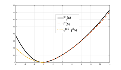
(a) $F_{\varepsilon}(s)$ vs $F(s):=\frac{1}{p(p-1)}s^{p}+\frac{p^{3}-4p^{2}+3p+2}{2p(p-1)^{2}}\varepsilon^{p}$

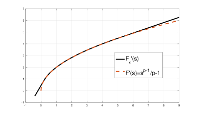
(b) $F^{\prime}_{\varepsilon}(s)$ vs $F^{\prime}(s):=\frac{1}{p-1}s^{p-1}$

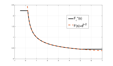
(c) $F^{\prime\prime}_{\varepsilon}(s)$ vs $F^{\prime\prime}(s):=s^{p-2}$

Figure 1: The function $F_{\varepsilon}$ and its derivatives.

Lemma 4.1.

The function $F_{\varepsilon}$ satisfies

$$F_{\varepsilon}(s)\geq\frac{\varepsilon^{p-2}s^{2}}{4}\qquad\forall s\leq\varepsilon\ \ \mbox{ and }\ \ F_{\varepsilon}(s)\geq Cs^{p}\qquad\forall s>\varepsilon,$$ (44)

where the constant $C>0$ is independent of $\varepsilon$.

Proof.

Since $F_{\varepsilon}\in C^{2}(\mathbb{R})$, using the Taylor formula as well as the definition of $F_{\varepsilon}$ and $F^{\prime}_{\varepsilon}$, we have that, for some $s_{0}\in\mathbb{R}$ between $0$ and $s$,

$$F_{\varepsilon}(s)=F_{\varepsilon}(0)+F^{\prime}_{\varepsilon}(0)s+\frac{1}{2}F^{\prime\prime}_{\varepsilon}(s_{0})s^{2}=\Big{(}\frac{2-p}{p-1}\Big{)}^{2}\varepsilon^{p}+\frac{2-p}{p-1}\varepsilon^{p-1}s+\frac{1}{2}F^{\prime\prime}_{\varepsilon}(s_{0})s^{2}.$$ (45)

Then, taking into account that $F^{\prime\prime}_{\varepsilon}(s)=\varepsilon^{p-2}$ for all $s\leq\varepsilon$, from (45) we have that: (a) if $s\in[0,\varepsilon]$, $F_{\varepsilon}(s)\geq\frac{1}{2}\varepsilon^{p-2}s^{2}$; and (b) if $s<0$, by using the Young inequality,

$$F_{\varepsilon}(s)\geq\Big{(}\frac{2-p}{p-1}\Big{)}^{2}\varepsilon^{p}-\frac{1}{4}\varepsilon^{p-2}s^{2}-\Big{(}\frac{2-p}{p-1}\Big{)}^{2}\varepsilon^{p}+\frac{1}{2}\varepsilon^{p-2}s^{2}=\frac{1}{4}\varepsilon^{p-2}s^{2},$$

from which we deduce (44)₁. Finally, (44)₂ follows directly from the definition of $F_{\varepsilon}$ for $s\geq\varepsilon$. ∎

Remark 4.2.

Notice that estimates in (44) imply that $|s|^{p}\leq K_{1}F_{\varepsilon}(s)+K_{2}$ for all $s\in\mathbb{R}$, where the constants $K_{1},K_{2}>0$ are independent of $\varepsilon$.

Then, taking into account the functions $F_{\varepsilon}$, its derivatives and $a_{\varepsilon}$, a regularized version of problem (2) reads: Find $u_{\varepsilon}:\Omega\times[0,T]\rightarrow\mathbb{R}$ and $v_{\varepsilon}:\Omega\times[0,T]\rightarrow\mathbb{R}$, with $u_{\varepsilon},v_{\varepsilon}\geq 0$, such that

$$\left\{\begin{array}[c]{lll}\partial_{t}u_{\varepsilon}-\Delta u_{\varepsilon}-\nabla\cdot(a_{\varepsilon}(u_{\varepsilon})\nabla v_{\varepsilon})=0\ \ \mbox{in}\ \Omega,\ t>0,\\ \partial_{t}{v}_{\varepsilon}-\Delta v_{\varepsilon}+{v}_{\varepsilon}=p(p-1)F_{\varepsilon}(u_{\varepsilon})\ \ \mbox{in}\ \Omega,\ t>0,\\ \displaystyle\frac{\partial u_{\varepsilon}}{\partial\mathbf{n}}=\frac{\partial v_{\varepsilon}}{\partial\mathbf{n}}=0\ \ \mbox{on}\ \partial\Omega,\ t>0,\\ u_{\varepsilon}(\textit{{x}},0)=u_{0}(\textit{{x}})\geq 0,\ v_{\varepsilon}(\textit{{x}},0)=v_{0}(\textit{{x}})\geq 0\ \ \mbox{in}\ \Omega.\end{array}\right.$$ (46)

Remark 4.3.

The idea is to define a fully discrete scheme associated to (46), taking in general $\varepsilon=\varepsilon(k,h)$, such that $\varepsilon(k,h)\rightarrow 0$ as $(k,h)\rightarrow 0$, where $k$ is the time step and $h$ the mesh size.

Observe that (formally) multiplying (46)₁ by $pF^{\prime}_{\varepsilon}(u_{\varepsilon})$, (46)₂ by $-\Delta v_{\varepsilon}$, integrating over $\Omega$ and adding, the chemotaxis and production terms cancel and we obtain the following energy law

$$\frac{d}{dt}\displaystyle\int_{\Omega}\Big{(}pF_{\varepsilon}(u_{\varepsilon})+\frac{1}{2}|\nabla v_{\varepsilon}|^{2}\Big{)}d\textit{{x}}+\int_{\Omega}pF^{\prime\prime}_{\varepsilon}(u_{\varepsilon})|\nabla u_{\varepsilon}|^{2}d\textit{{x}}+\|\nabla v_{\varepsilon}\|_{1}^{2}=0.$$

In particular, the modified energy

$$\mathcal{E}_{\varepsilon}(u,v)=\displaystyle\int_{\Omega}\Big{(}pF_{\varepsilon}(u)+\frac{1}{2}|\nabla v|^{2}\Big{)}d\textit{{x}}$$

is decreasing in time. Thus, we consider a fully discrete approximation of the regularized problem (46) using a FE discretization in space and the backward Euler discretization in time (considered for simplicity on a uniform partition of $[0,T]$ with time step $k=T/N:(t_{n}=nk)_{n=0}^{n=N}$). Let $\Omega$ be a polygonal domain. We consider a shape-regular and quasi-uniform family of triangulations of $\Omega$, denoted by $\{\mathcal{T}_{h}\}_{h>0}$, with simplices $K$, $h_{K}=diam(K)$ and $h:=\max_{K\in\mathcal{T}_{h}}h_{K}$, so that $\overline{\Omega}=\cup_{K\in\mathcal{T}_{h}}\overline{K}$. Further, let $\mathcal{N}_{h}=\{\mathbf{a}_{i}\}_{i\in\mathcal{I}}$ denote the set of all the vertices of $\mathcal{T}_{h}$, and in this case we will assume the following hypothesis:

1. The triangulation is structured in the sense that all simplices have a right angle.

We choose the following continuous FE spaces for $u_{\varepsilon}$ and $v_{\varepsilon}$:

$$(U_{h},V_{h})\subset H^{1}(\Omega)^{2},\quad\hbox{generated by $\mathbb{P}_{1},\mathbb{P}_{r}$ with $r\geq 1$.}$$

Remark 4.4.

The right-angled constraint (H) and the approximation of $U_{h}$ by $\mathbb{P}_{1}$-continuous FE are necessary to obtain the relations (49)-(50) below, which are essential in order to obtain the energy-stability of the scheme UV$\varepsilon$ (see Theorem 4.9 below).

We denote the Lagrange interpolation operator by $\Pi^{h}:C(\overline{\Omega})\rightarrow U_{h}$, and we introduce the discrete semi-inner product on $C(\overline{\Omega})$ (which is an inner product in $U_{h}$) and its induced discrete seminorm (norm in $U_{h}$):

$$(u_{1},u_{2})^{h}:=\int_{\Omega}\Pi^{h}(u_{1}u_{2}),\ ~~|u|_{h}=\sqrt{(u,u)^{h}}.$$ (47)

Remark 4.5.

In $U_{h}$, the norms $|\cdot|_{h}$ and $\|\cdot\|_{0}$ are equivalents uniformly with respect to $h$ (see [5]).

We consider also the $L^{2}$-projection $Q^{h}:L^{2}(\Omega)\rightarrow U_{h}$ given by

$$(Q^{h}u,\bar{u})^{h}=(u,\bar{u}),\ \ \forall\bar{u}\in U_{h},$$ (48)

and the standard $H^{1}$-projection ${R}^{h}:H^{1}(\Omega)\rightarrow V_{h}$. Moreover, owing to the right angled constraint (H) and the choice of $\mathbb{P}_{1}$-continuous FE for $U_{h}$, following the ideas of [3] (see also [12]), for each $\varepsilon\in(0,1)$, we can construct two operators $\Lambda^{i}_{\varepsilon}:U_{h}\rightarrow L^{\infty}(\Omega)^{d\times d}$ ($i=1,2$) such that $\Lambda_{\varepsilon}^{i}u^{h}$ are symmetric matrices and $\Lambda_{\varepsilon}^{1}u^{h}$ is positive definite, for all $u^{h}\in U_{h}$ and a.e. in $\Omega$, and satisfy

$$(\Lambda^{1}_{\varepsilon}u^{h})\nabla\Pi^{h}(F^{\prime}_{\varepsilon}(u^{h}))=\nabla u^{h}\ \ \mbox{ in }\Omega,$$ (49)

$$(\Lambda^{2}_{\varepsilon}u^{h})\nabla\Pi^{h}(F^{\prime}_{\varepsilon}(u^{h}))=(p-1)\nabla\Pi^{h}(F_{\varepsilon}(u^{h}))\ \ \mbox{ in }\Omega.$$ (50)

Basically, $\Lambda^{i}_{\varepsilon}u^{h}$ ($i=1,2$) are constant by elements matrices such that (49) and (50) holds by elements. In the $1$-dimensional case, $\Lambda_{\varepsilon}^{i}$ are constructed as follows: For all $u^{h}\in U_{h}$ and $K\in\mathcal{T}_{h}$ with vertices $\mathbf{a}_{0}^{K}$ and $\mathbf{a}_{1}^{K}$, we set

$$\Lambda_{\varepsilon}^{1}(u^{h})|_{K}\ :=\left\{\begin{array}[]{lcl}\frac{u^{h}(\mathbf{a}_{1}^{K})-u^{h}(\mathbf{a}_{0}^{K})}{F^{\prime}_{\varepsilon}(u^{h}(\mathbf{a}_{1}^{K}))-F^{\prime}_{\varepsilon}(u^{h}(\mathbf{a}_{0}^{K}))}=\frac{1}{F^{\prime\prime}_{\varepsilon}(u^{h}(\xi))}&\mbox{ if }&u^{h}(\mathbf{a}_{0}^{K})\neq u^{h}(\mathbf{a}_{1}^{K}),\\ \frac{1}{F^{\prime\prime}_{\varepsilon}(u^{h}(\mathbf{a}_{0}^{K}))}&\mbox{ if }&u^{h}(\mathbf{a}_{0}^{K})=u^{h}(\mathbf{a}_{1}^{K}),\end{array}\right.$$ (51)

for some $\xi\in K$, and

$$\Lambda_{\varepsilon}^{2}(u^{h})|_{K}\!:=\!\left\{\begin{array}[]{lcl}(p-1)\frac{F_{\varepsilon}(u^{h}(\mathbf{a}_{1}^{K}))-F_{\varepsilon}(u^{h}(\mathbf{a}_{0}^{K}))}{F^{\prime}_{\varepsilon}(u^{h}(\mathbf{a}_{1}^{K}))-F^{\prime}_{\varepsilon}(u^{h}(\mathbf{a}_{0}^{K}))}=(p-1)\frac{F^{\prime}_{\varepsilon}(u^{h}(\xi_{1}))}{F^{\prime\prime}_{\varepsilon}(u^{h}(\xi_{2}))}&\mbox{if}&u^{h}(\mathbf{a}_{0}^{K})\neq u^{h}(\mathbf{a}_{1}^{K}),\\ (p-1)\frac{F^{\prime}_{\varepsilon}(u^{h}(\mathbf{a}_{0}^{K}))}{F^{\prime\prime}_{\varepsilon}(u^{h}(\mathbf{a}_{0}^{K}))}&\mbox{if}&u^{h}(\mathbf{a}_{0}^{K})=u^{h}(\mathbf{a}_{1}^{K}),\end{array}\right.$$ (52)

for some $\xi_{1},\xi_{2}\in K$. Following [3] (see also [12]), these constructions can be extended to dimensions 2 and 3, and from (51) the following estimate holds:

$$\varepsilon^{2-p}\xi^{T}\xi\leq\xi^{T}\Lambda^{1}_{\varepsilon}(u^{h})^{-1}\xi\leq\varepsilon^{p-2}\xi^{T}\xi,\ \ \forall\xi\in\mathbb{R}^{d},\ u^{h}\in U_{h}.$$ (53)

Now, we prove the following result which will be used in order to prove the well-posedness of the scheme UV$\varepsilon$.

Lemma 4.6.

Let $\|\cdot\|$ denote the spectral norm on $\mathbb{R}^{d\times d}$. Then for any given $\varepsilon\in(0,1)$ the function $\Lambda_{\varepsilon}^{2}:U_{h}\rightarrow[L^{\infty}(\Omega)]^{d\times d}$ satisfies, for all $u^{h}_{1},u^{h}_{2}\in U_{h}$ and $K\in\mathcal{T}_{h}$ with vertices $\{\mathbf{a}_{l}^{K}\}_{l=0}^{d}$,

$$\!\!\!\!\!\!\|(\Lambda^{2}_{\varepsilon}(u^{h}_{1})-\Lambda^{2}_{\varepsilon}(u^{h}_{2}))|_{K}\|$$

$$\hskip 11.38092pt\!\!\!\!\!\!\leq 3\varepsilon^{2(p-2)}\max\{1,(p-1)\varepsilon^{2(p-2)}\}\max_{l=1,...,d}\{|u^{h}_{1}(\mathbf{a}_{l}^{K})-u^{h}_{2}(\mathbf{a}_{l}^{K}))|+|u^{h}_{1}(\mathbf{a}_{0}^{K})-u^{h}_{2}(\mathbf{a}_{0}^{K})|\},$$ (54)

where $\mathbf{a}^{K}_{0}$ is the right-angled vertex.

Proof.

The proof follows the ideas of [4, Lemma 2.1], with some modifications. For simplicity in the notation, we will prove (4.6) in the 1-dimensional case, but this proof can be extended to dimensions 2 and 3 as in [4, Lemma 2.1]. Observe that, from (52)

$$\|(\Lambda^{2}_{\varepsilon}(u^{h}_{1})-\Lambda^{2}_{\varepsilon}(u^{h}_{2}))|_{K}\| \!\!\!\leq|(\Lambda^{2}_{\varepsilon}(u^{h}_{1})-\Lambda^{2}_{\varepsilon}(u^{h}_{1,2}))|_{K}|+|(\Lambda^{2}_{\varepsilon}(u^{h}_{1,2})-\Lambda^{2}_{\varepsilon}(u^{h}_{2}))|_{K}|$$ (55)

$$=(p-1)\left|\frac{F^{\prime}_{\varepsilon}(\mu_{11})}{F^{\prime\prime}_{\varepsilon}(\mu_{12})}-\frac{F^{\prime}_{\varepsilon}(\xi_{1})}{F^{\prime\prime}_{\varepsilon}(\xi_{2})}\right|+(p-1)\left|\frac{F^{\prime}_{\varepsilon}(\xi_{1})}{F^{\prime\prime}_{\varepsilon}(\xi_{2})}-\frac{F^{\prime}_{\varepsilon}(\mu_{21})}{F^{\prime\prime}_{\varepsilon}(\mu_{22})}\right|,$$

where $u^{h}_{1,2}\in\mathbb{P}_{1}(K)$ with $u^{h}_{1,2}(\mathbf{a}_{0}^{K})=u^{h}_{2}(\mathbf{a}_{0}^{K})$ and $u^{h}_{1,2}(\mathbf{a}_{1}^{K})=u^{h}_{1}(\mathbf{a}_{1}^{K})$, $\mu_{1i}$ ($i=1,2$) lie between $u^{h}_{1}(\mathbf{a}_{0}^{K})$ and $u^{h}_{1}(\mathbf{a}_{1}^{K})$, $\mu_{2i}$ ($i=1,2$) lie between $u^{h}_{2}(\mathbf{a}_{0}^{K})$ and $u^{h}_{2}(\mathbf{a}_{1}^{K})$, and $\xi_{i}$ ($i=1,2$) lie between $u^{h}_{1}(\mathbf{a}_{1}^{K})$ and $u^{h}_{2}(\mathbf{a}_{0}^{K})$. Then, first we will show that

$$(p-1)\left|\frac{F^{\prime}_{\varepsilon}(\mu_{11})}{F^{\prime\prime}_{\varepsilon}(\mu_{12})}-\frac{F^{\prime}_{\varepsilon}(\xi_{1})}{F^{\prime\prime}_{\varepsilon}(\xi_{2})}\right|\leq 3\varepsilon^{2(p-2)}\max\{1,(p-1)\varepsilon^{2(p-2)}\}|u^{h}_{1}(\mathbf{a}_{0}^{K})-u^{h}_{2}(\mathbf{a}_{0}^{K})|,$$ (56)

for $u^{h}_{1}(\mathbf{a}_{0}^{K})\neq u^{h}_{2}(\mathbf{a}_{0}^{K})$, because the case $u^{h}_{1}(\mathbf{a}_{0}^{K})=u^{h}_{2}(\mathbf{a}_{0}^{K})$ is trivially true. With this aim, we consider $\gamma_{i}$ ($i=1,2$) lying between $u^{h}_{1}(\mathbf{a}_{0}^{K})$ and $u^{h}_{2}(\mathbf{a}_{0}^{K})$ such that

$$F^{\prime}_{\varepsilon}(\gamma_{1})=\frac{F_{\varepsilon}(u^{h}_{2}(\mathbf{a}_{0}^{K}))-F_{\varepsilon}(u^{h}_{1}(\mathbf{a}_{0}^{K}))}{u^{h}_{2}(\mathbf{a}_{0}^{K})-u^{h}_{1}(\mathbf{a}_{0}^{K})}\ \ \mbox{ and }\ \ F^{\prime\prime}_{\varepsilon}(\gamma_{2})=\frac{F^{\prime}_{\varepsilon}(u^{h}_{2}(\mathbf{a}_{0}^{K}))-F^{\prime}_{\varepsilon}(u^{h}_{1}(\mathbf{a}_{0}^{K}))}{u^{h}_{2}(\mathbf{a}_{0}^{K})-u^{h}_{1}(\mathbf{a}_{0}^{K})},$$ (57)

and therefore, from the definitions of $\xi_{i}$, $\gamma_{i}$ and $\mu_{1i}$, $i=1,2$, given after (55) and (57), we deduce

$$(u^{h}_{2}(\mathbf{a}_{0}^{K})-u^{h}_{1}(\mathbf{a}_{0}^{K}))F^{\prime}_{\varepsilon}(\gamma_{1})=(u^{h}_{2}(\mathbf{a}_{0}^{K})-u^{h}_{1}(\mathbf{a}_{1}^{K}))F^{\prime}_{\varepsilon}(\xi_{1})+(u^{h}_{1}(\mathbf{a}_{1}^{K})-u^{h}_{1}(\mathbf{a}_{0}^{K}))F^{\prime}_{\varepsilon}(\mu_{11}),$$ (58)

$$(u^{h}_{2}(\mathbf{a}_{0}^{K})-u^{h}_{1}(\mathbf{a}_{0}^{K}))F^{\prime\prime}_{\varepsilon}(\gamma_{2})=(u^{h}_{2}(\mathbf{a}_{0}^{K})-u^{h}_{1}(\mathbf{a}_{1}^{K}))F^{\prime\prime}_{\varepsilon}(\xi_{2})+(u^{h}_{1}(\mathbf{a}_{1}^{K})-u^{h}_{1}(\mathbf{a}_{0}^{K}))F^{\prime\prime}_{\varepsilon}(\mu_{12}).$$ (59)

Then, for $u^{h}_{2}(\mathbf{a}_{0}^{K})$, $u^{h}_{1}(\mathbf{a}_{0}^{K})$ and $u^{h}_{1}(\mathbf{a}_{1}^{K})$, there are only 3 options: (1) $u^{h}_{1}(\mathbf{a}_{1}^{K})$ lies between $u^{h}_{2}(\mathbf{a}_{0}^{K})$ and $u^{h}_{1}(\mathbf{a}_{0}^{K})$; (ii) $u^{h}_{2}(\mathbf{a}_{0}^{K})$ lies between $u^{h}_{1}(\mathbf{a}_{1}^{K})$ and $u^{h}_{1}(\mathbf{a}_{0}^{K})$; and (iii) $u^{h}_{1}(\mathbf{a}_{0}^{K})$ lies between $u^{h}_{1}(\mathbf{a}_{1}^{K})$ and $u^{h}_{2}(\mathbf{a}_{0}^{K})$.

Notice that from (42)-(43), we have that $F^{\prime}_{\varepsilon}$ and $(p-1)\frac{F^{\prime}_{\varepsilon}}{F^{\prime\prime}_{\varepsilon}}$ are globally Lipschitz functions with constants $\varepsilon^{p-2}$ and $1$ respectively, and $\frac{1}{|F^{\prime\prime}_{\varepsilon}|}\leq\varepsilon^{p-2}$. Then, in case (i), taking into account that all intermediate values $\mu_{1i},\gamma_{i},\xi_{i}$ ($i=1,2$) lie between $u^{h}_{2}(\mathbf{a}_{0}^{K})$ and $u^{h}_{1}(\mathbf{a}_{0}^{K})$, we have

$$(p-1) \!\!\!\left|\frac{F^{\prime}_{\varepsilon}(\mu_{11})}{F^{\prime\prime}_{\varepsilon}(\mu_{12})}-\frac{F^{\prime}_{\varepsilon}(\xi_{1})}{F^{\prime\prime}_{\varepsilon}(\xi_{2})}\right|\leq(p-1)\left|\frac{F^{\prime}_{\varepsilon}(\mu_{11})-F^{\prime}_{\varepsilon}(\mu_{12})}{F^{\prime\prime}_{\varepsilon}(\mu_{12})}\right|$$ (60)

$$\!\!\!+(p-1)\left|\frac{F^{\prime}_{\varepsilon}(\mu_{12})}{F^{\prime\prime}_{\varepsilon}(\mu_{12})}-\frac{F^{\prime}_{\varepsilon}(\xi_{2})}{F^{\prime\prime}_{\varepsilon}(\xi_{2})}\right|+(p-1)\left|\frac{F^{\prime}_{\varepsilon}(\xi_{1})-F^{\prime}_{\varepsilon}(\xi_{2})}{F^{\prime\prime}_{\varepsilon}(\xi_{2})}\right|$$

$$\!\!\!\leq(p-1)\varepsilon^{2(p-2)}|\mu_{11}-\mu_{12}|+|\mu_{12}-\xi_{2}|+(p-1)\varepsilon^{2(p-2)}|\xi_{1}-\xi_{2}|$$

$$\!\!\!\leq 3\max\{1,(p-1)\varepsilon^{2(p-2)}\}|u^{h}_{1}(\mathbf{a}_{0}^{K})-u^{h}_{2}(\mathbf{a}_{0}^{K})|.$$

In case (ii), all intermediate values $\mu_{1i},\gamma_{i},\xi_{i}$ ($i=1,2$) lie between $u^{h}_{1}(\mathbf{a}_{1}^{K})$ and $u^{h}_{1}(\mathbf{a}_{0}^{K})$, and from (58)-(59) by eliminating the term $(u^{h}_{2}(\mathbf{a}_{0}^{K})-u^{h}_{1}(\mathbf{a}_{1}^{K}))$, we have the equality

$$(u^{h}_{1}(\mathbf{a}_{1}^{K})-u^{h}_{1}(\mathbf{a}_{0}^{K}))\left[\frac{F^{\prime}_{\varepsilon}(\xi_{1})}{F^{\prime\prime}_{\varepsilon}(\xi_{2})}-\frac{F^{\prime}_{\varepsilon}(\mu_{11})}{F^{\prime\prime}_{\varepsilon}(\mu_{12})}\right]=(u^{h}_{2}(\mathbf{a}_{0}^{K})-u^{h}_{1}(\mathbf{a}_{0}^{K}))\frac{F^{\prime\prime}_{\varepsilon}(\gamma_{2})}{F^{\prime\prime}_{\varepsilon}(\mu_{12})}\left[\frac{F^{\prime}_{\varepsilon}(\xi_{1})}{F^{\prime\prime}_{\varepsilon}(\xi_{2})}-\frac{F^{\prime}_{\varepsilon}(\gamma_{1})}{F^{\prime\prime}_{\varepsilon}(\gamma_{2})}\right],$$

from which, bounding the term $\left|\frac{F^{\prime}_{\varepsilon}(\xi_{1})}{F^{\prime\prime}_{\varepsilon}(\xi_{2})}-\frac{F^{\prime}_{\varepsilon}(\gamma_{1})}{F^{\prime\prime}_{\varepsilon}(\gamma_{2})}\right|$ as in (60), we obtain

$$(p-1) \!\!\!|u^{h}_{1}(\mathbf{a}_{1}^{K})-u^{h}_{1}(\mathbf{a}_{0}^{K}))|\left|\frac{F^{\prime}_{\varepsilon}(\mu_{11})}{F^{\prime\prime}_{\varepsilon}(\mu_{12})}-\frac{F^{\prime}_{\varepsilon}(\xi_{1})}{F^{\prime\prime}_{\varepsilon}(\xi_{2})}\right|$$

$$\!\!\!\!\!\leq\varepsilon^{2(p-2)}3\max\{1,(p-1)\varepsilon^{2(p-2)}\}|u^{h}_{1}(\mathbf{a}_{0}^{K})-u^{h}_{2}(\mathbf{a}_{0}^{K})||u^{h}_{1}(\mathbf{a}_{1}^{K})-u^{h}_{1}(\mathbf{a}_{0}^{K}))|,$$

and therefore, dividing by $|u^{h}_{1}(\mathbf{a}_{1}^{K})-u^{h}_{1}(\mathbf{a}_{0}^{K}))|$ we arrive at

$$(p-1)\left|\frac{F^{\prime}_{\varepsilon}(\mu_{11})}{F^{\prime\prime}_{\varepsilon}(\mu_{12})}-\frac{F^{\prime}_{\varepsilon}(\xi_{1})}{F^{\prime\prime}_{\varepsilon}(\xi_{2})}\right|\leq 3\varepsilon^{2(p-2)}\max\{1,(p-1)\varepsilon^{2(p-2)}\}|u^{h}_{1}(\mathbf{a}_{0}^{K})-u^{h}_{2}(\mathbf{a}_{0}^{K})|.$$ (61)

In case (iii), by arguing analogously to case (ii), from (58)-(59) we have

$$(u^{h}_{1}(\mathbf{a}_{1}^{K})-u^{h}_{2}(\mathbf{a}_{0}^{K}))\left[\frac{F^{\prime}_{\varepsilon}(\xi_{1})}{F^{\prime\prime}_{\varepsilon}(\xi_{2})}-\frac{F^{\prime}_{\varepsilon}(\mu_{11})}{F^{\prime\prime}_{\varepsilon}(\mu_{12})}\right]=(u^{h}_{2}(\mathbf{a}_{0}^{K})-u^{h}_{1}(\mathbf{a}_{0}^{K}))\frac{F^{\prime\prime}_{\varepsilon}(\gamma_{2})}{F^{\prime\prime}_{\varepsilon}(\xi_{2})}\left[\frac{F^{\prime}_{\varepsilon}(\gamma_{1})}{F^{\prime\prime}_{\varepsilon}(\gamma_{2})}-\frac{F^{\prime}_{\varepsilon}(\mu_{11})}{F^{\prime\prime}_{\varepsilon}(\mu_{12})}\right],$$

which implies (61). Therefore, we have proved (56). Analogously, we can prove that

$$(p-1)\left|\frac{F^{\prime}_{\varepsilon}(\xi_{1})}{F^{\prime\prime}_{\varepsilon}(\xi_{2})}-\frac{F^{\prime}_{\varepsilon}(\mu_{21})}{F^{\prime\prime}_{\varepsilon}(\mu_{22})}\right|\leq 3\varepsilon^{2(p-2)}\max\{1,(p-1)\varepsilon^{2(p-2)}\}|u^{h}_{1}(\mathbf{a}_{1}^{K})-u^{h}_{2}(\mathbf{a}_{1}^{K})|.$$ (62)

Thus, from (55), (56) and (62) we conclude (4.6). ∎

Let $A_{h}:V_{h}\rightarrow V_{h}$ be the linear operator defined as follows

$$(A_{h}v^{h},\bar{v})=(\nabla v^{h},\nabla\bar{v})+(v^{h},\bar{v}),\ \ \forall\bar{v}\in V_{h}.$$

Then, the following estimate holds (see for instance, [14, Theorem 3.2]):

$$\|v^{h}\|_{W^{1,6}}\leq C\|A_{h}v^{h}\|_{0},\ \ \forall v^{h}\in V_{h}.$$ (63)

Thus, we consider the following first order in time, nonlinear and coupled scheme:

• Scheme UV$\varepsilon$:
  Initialization: Let $(u^{0},v^{0})=(Q^{h}u_{0},R^{h}v_{0})\in U_{h}\times V_{h}$.
  Time step n: Given $(u^{n-1}_{\varepsilon},v^{n-1}_{\varepsilon})\in U_{h}\times V_{h}$, compute $(u^{n}_{\varepsilon},v^{n}_{\varepsilon})\in U_{h}\times V_{h}$ solving

  $$\left\{\begin{array}[c]{lll}(\delta_{t}u^{n}_{\varepsilon},\bar{u})^{h}+(\nabla u^{n}_{\varepsilon},\nabla\bar{u})=-(\Lambda_{\varepsilon}^{2}(u^{n}_{\varepsilon})\nabla v^{n}_{\varepsilon},\nabla\bar{u}),\ \ \forall\bar{u}\in U_{h},\\ (\delta_{t}{v}^{n}_{\varepsilon},\bar{v})+(A_{h}v^{n}_{\varepsilon},\bar{v})=p(p-1)(\Pi^{h}(F_{\varepsilon}(u^{n}_{\varepsilon})),\bar{v}),\ \ \forall\bar{v}\in V_{h},\end{array}\right.$$ (64)

where, in general, we denote $\delta_{t}a^{n}:=\displaystyle\frac{a^{n}-a^{n-1}}{k}$.

Remark 4.7.

(Positivity of $v^{n}_{\varepsilon}$) By using the mass-lumping technique in all terms of (64)₂ excepting the self-diffusion term $(\nabla v^{n}_{\varepsilon},\nabla\bar{v})$, and approximating $V_{h}$ by $\mathbb{P}_{1}$-continuous FE, we can prove that if $v^{n-1}_{\varepsilon}\geq 0$ then $v^{n}_{\varepsilon}\geq 0$. In fact, it follows testing (64)₂ by $\bar{v}=\Pi^{h}(v^{n}_{\varepsilon-})\in V_{h}$, where $v^{n}_{\varepsilon-}:=\min\{v^{n}_{\varepsilon},0\}$ (see Remark 3.10 in [15]).

4.1.1 Mass-conservation, Energy-stability and Solvability

Since $\bar{u}=1\in U_{h}$ and $\bar{v}=1\in V_{h}$, we deduce that the scheme UV$\varepsilon$ is conservative in $u^{n}_{\varepsilon}$, that is,

$$(u_{\varepsilon}^{n},1)=(u^{n}_{\varepsilon},1)^{h}=(u^{n-1}_{\varepsilon},1)^{h}=\cdot\cdot\cdot=(u^{0},1)^{h}=(u^{0},1)=(Q^{h}u_{0},1)=(u_{0},1):=m_{0},$$ (65)

and we have the following behavior for $\int_{\Omega}v^{n}_{\varepsilon}$:

$$\delta_{t}\left(\int_{\Omega}v^{n}_{\varepsilon}\right)=p(p-1)\int_{\Omega}\Pi^{h}(F_{\varepsilon}(u^{n}_{\varepsilon}))-\int_{\Omega}v^{n}_{\varepsilon}.$$ (66)

Definition 4.8.

A numerical scheme with solution $(u^{n}_{\varepsilon},v^{n}_{\varepsilon})$ is called energy-stable with respect to the energy

$$\mathcal{E}_{\varepsilon}^{h}(u,v)=p(F_{\varepsilon}(u),1)^{h}+\frac{1}{2}\|\nabla v\|_{0}^{2}$$ (67)

if this energy is time decreasing, that is $\mathcal{E}_{\varepsilon}^{h}(u^{n}_{\varepsilon},v^{n}_{\varepsilon})\leq\mathcal{E}_{\varepsilon}^{h}(u^{n-1}_{\varepsilon},v^{n-1}_{\varepsilon})$ for all $n\geq 1$.

Theorem 4.9.

(Unconditional stability) The scheme UV$\varepsilon$ is unconditionally energy stable with respect to $\mathcal{E}_{\varepsilon}^{h}(u,v)$. In fact, if $(u^{n}_{\varepsilon},v^{n}_{\varepsilon})$ is a solution of UV$\varepsilon$, then the following discrete energy law holds

$$\delta_{t}\mathcal{E}_{\varepsilon}^{h}(u^{n}_{\varepsilon},v^{n}_{\varepsilon})+\frac{k\varepsilon^{2-p}p}{2}\|\delta_{t}u^{n}_{\varepsilon}\|_{0}^{2}+\frac{k}{2}\|\delta_{t}\nabla v^{n}_{\varepsilon}\|_{0}^{2}+p\varepsilon^{2-p}\|\nabla u^{n}_{\varepsilon}\|_{0}^{2}+\|(A_{h}-I)\nabla v^{n}_{\varepsilon}\|_{0}^{2}+\|\nabla v^{n}_{\varepsilon}\|_{0}^{2}\leq 0.$$ (68)

Proof.

Testing (64)₁ by $\bar{u}=p\Pi^{h}(F^{\prime}_{\varepsilon}(u^{n}_{\varepsilon}))$ and (64)₂ by $\bar{v}=(A_{h}-I)v^{n}_{\varepsilon}$, adding and taking into account that $\Lambda_{\varepsilon}^{i}(u^{n}_{\varepsilon})$ are symmetric as well as (49)-(50), the terms $-p(\Lambda^{2}_{\varepsilon}(u^{n}_{\varepsilon})\nabla v^{n}_{\varepsilon},\nabla\Pi^{h}(F^{\prime}_{\varepsilon}(u^{n}_{\varepsilon})))=-p(\nabla v^{n}_{\varepsilon},\Lambda^{2}_{\varepsilon}(u^{n}_{\varepsilon})\nabla\Pi^{h}(F^{\prime}_{\varepsilon}(u^{n}_{\varepsilon})))=-p(p-1)(\nabla v^{n}_{\varepsilon},\nabla\Pi^{h}(F_{\varepsilon}(u^{n}_{\varepsilon})))$ and $p(p-1)(\Pi^{h}(F_{\varepsilon}(u^{n}_{\varepsilon})),(A_{h}-I)v^{n}_{\varepsilon})=p(p-1)(\nabla\Pi^{h}(F_{\varepsilon}(u^{n}_{\varepsilon})),\nabla v^{n}_{\varepsilon})$ cancel, and using that $\nabla\Pi^{h}(F^{\prime}_{\varepsilon}(u^{n}_{\varepsilon}))=\Lambda_{\varepsilon}^{1}(u^{n}_{\varepsilon})^{-1}\nabla u^{n}_{\varepsilon}$ we obtain

$$p(\delta_{t}u^{n}_{\varepsilon},F^{\prime}_{\varepsilon}(u^{n}_{\varepsilon}))^{h} \!\!\!\!+p\int_{\Omega}(\nabla u^{n}_{\varepsilon})^{T}\!\cdot\!\Lambda_{\varepsilon}^{1}(u^{n}_{\varepsilon})^{-1}\!\cdot\!\nabla u^{n}_{\varepsilon}d\textit{{x}}$$ (69)

$$\!\!\!\!+\delta_{t}\Big{(}\frac{1}{2}\|\nabla v^{n}_{\varepsilon}\|_{0}^{2}\Big{)}+\frac{k}{2}\|\delta_{t}\nabla v^{n}_{\varepsilon}\|_{0}^{2}+\|(A_{h}-I)v^{n}_{\varepsilon}\|_{0}^{2}+\|\nabla v^{n}_{\varepsilon}\|_{0}^{2}=0.$$

Moreover, observe that from the Taylor formula we have

$$F_{\varepsilon}(u^{n-1}_{\varepsilon})=F_{\varepsilon}(u^{n}_{\varepsilon})+F^{\prime}_{\varepsilon}(u^{n}_{\varepsilon})(u^{n-1}_{\varepsilon}-u^{n}_{\varepsilon})+\frac{1}{2}F^{\prime\prime}_{\varepsilon}(\theta u^{n}_{\varepsilon}+(1-\theta)u^{n-1}_{\varepsilon})(u^{n-1}_{\varepsilon}-u^{n}_{\varepsilon})^{2},$$

and therefore,

$$\delta_{t}u^{n}_{\varepsilon}\cdot F^{\prime}_{\varepsilon}(u^{n}_{\varepsilon})=\delta_{t}\Big{(}F_{\varepsilon}(u^{n}_{\varepsilon})\Big{)}+\frac{k}{2}F^{\prime\prime}_{\varepsilon}(\theta u^{n}_{\varepsilon}+(1-\theta)u^{n-1}_{\varepsilon})(\delta_{t}u^{n}_{\varepsilon})^{2}.$$ (70)

Then, using (70) and taking into account that $\Pi^{h}$ is linear and $F^{\prime\prime}_{\varepsilon}(s)\geq\varepsilon^{2-p}$ for all $s\in\mathbb{R}$, we have

$$(\delta_{t}u^{n}_{\varepsilon},F^{\prime}_{\varepsilon}(u^{n}_{\varepsilon}))^{h} \!\!\!=\delta_{t}\Big{(}\int_{\Omega}\Pi^{h}(F_{\varepsilon}(u^{n}_{\varepsilon}))\Big{)}+\frac{k}{2}\int_{\Omega}\Pi^{h}(F^{\prime\prime}_{\varepsilon}(\theta u^{n}_{\varepsilon}+(1-\theta)u^{n-1}_{\varepsilon})(\delta_{t}u^{n}_{\varepsilon})^{2})$$ (71)

$$\!\!\!\geq\delta_{t}\Big{(}(F_{\varepsilon}(u^{n}_{\varepsilon}),1)^{h}\Big{)}+\frac{k\varepsilon^{2-p}}{2}|\delta_{t}u^{n}_{\varepsilon}|_{h}^{2}.$$

Thus, from (69), (53), (71) and Remark 4.5, we arrive at (68). ∎

Corollary 4.10.

(Uniform estimates) Assume that $(u_{0},v_{0})\in L^{2}(\Omega)\times H^{1}(\Omega)$. Let $(u^{n}_{\varepsilon},v^{n}_{\varepsilon})$ be a solution of scheme UV$\varepsilon$. Then, it holds

$$p(F_{\varepsilon}(u^{n}_{\varepsilon}),1)^{h}+\frac{1}{2}\|v^{n}_{\varepsilon}\|_{1}^{2}+k\underset{m=1}{\overset{n}{\sum}}\left(p\varepsilon^{2-p}\|\nabla u^{m}_{\varepsilon}\|_{0}^{2}+\|(A_{h}-I)v^{m}_{\varepsilon}\|_{0}^{2}+\|\nabla v^{m}_{\varepsilon}\|_{0}^{2}\right)\leq\frac{C_{0}}{(p-1)^{2}},\ \ \forall n\geq 1,$$ (72)

$$k\underset{m=n_{0}+1}{\overset{n+n_{0}}{\sum}}\|v^{m}_{\varepsilon}\|_{W^{1,6}}^{2}\leq\frac{C_{1}}{(p-1)^{2}}(1+kn),\ \ \forall n\geq 1,$$ (73)

where the integer $n_{0}\geq 0$ is arbitrary, with the constants $C_{0},C_{1}>0$ depending on the data $(\Omega,u_{0},v_{0})$, but independent of $k,h,n$ and $\varepsilon$. Moreover,

$$\|\Pi^{h}(u^{n}_{\varepsilon-})\|_{0}^{2}\leq\frac{C_{0}}{(p-1)^{2}}\varepsilon^{2-p}\ \ \mbox{ and}\ \ \|u^{n}_{\varepsilon}\|_{L^{p}}^{p}\leq\frac{C_{0}K}{(p-1)^{2}}+K,\ \ \forall n\geq 1,$$ (74)

where $u^{n}_{\varepsilon-}:=\min\{u^{n}_{\varepsilon},0\}\leq 0$ and the constant $K>0$ is independent of $k,h,n$ and $\varepsilon$.

Remark 4.11.

(Approximated positivity of $u^{n}_{\varepsilon}$) From (74)₁, the following estimate holds

$$\max_{n\geq 0}\|\Pi^{h}(u^{n}_{\varepsilon-})\|_{0}^{2}\leq\frac{C_{0}}{(p-1)^{2}}\varepsilon^{2-p}.$$

Proof.

First, taking into account that $(u^{0},{v}^{0})=(Q^{h}u_{0},R^{h}v_{0})$, $u_{0}\geq 0$ (and therefore, $u^{0}\geq 0$), as well as the definition of $F_{\varepsilon}$, we have that

$$\mathcal{E}^{h}_{\varepsilon}(u^{0},v^{0}) \!\!\!=p\int_{\Omega}\Pi^{h}(F_{\varepsilon}(u^{0}))+\frac{1}{2}\|\nabla v^{0}\|_{0}^{2}\leq\frac{C}{p-1}\int_{\Omega}\Pi^{h}\Big{(}(u^{0})^{2}+\frac{1}{p-1}\Big{)}+\frac{1}{2}\|\nabla v^{0}\|_{0}^{2}$$ (75)

$$\!\!\!\!\!\!\!\!\!\!\!\!\!\!\!\!\!\leq\frac{C}{p-1}\Big{(}\|u^{0}\|_{0}^{2}+\|\nabla v^{0}\|_{0}^{2}+\frac{1}{p-1}\Big{)}\leq\frac{C}{p-1}\Big{(}\|u_{0}\|_{0}^{2}+\|v_{0}\|_{1}^{2}+\frac{1}{p-1}\Big{)}\leq\frac{C_{0}}{(p-1)^{2}},$$

where the constant $C_{0}>0$ depends on the data $(\Omega,u_{0},v_{0})$, but is independent of $k,h,n$ and $\varepsilon$. Therefore, from the discrete energy law (68) and estimate (75), we have

$$\mathcal{E}^{h}_{\varepsilon}(u^{n}_{\varepsilon},v^{n}_{\varepsilon})+k\underset{m=1}{\overset{n}{\sum}}\left(p\varepsilon^{2-p}\|\nabla u^{m}_{\varepsilon}\|_{0}^{2}+\|(A_{h}-I)v^{m}_{\varepsilon}\|_{0}^{2}+\|\nabla v^{m}_{\varepsilon}\|_{0}^{2}\right)\leq\mathcal{E}^{h}_{\varepsilon}(u^{0},v^{0})\leq\frac{C_{0}}{(p-1)^{2}}.$$ (76)

Moreover, from (66), the definition of $F_{\varepsilon}$, Remark 4.2 and (76), we have

$$(1+k)\displaystyle\left|\int_{\Omega}v^{n}_{\varepsilon}\right|-\left|\int_{\Omega}v^{n-1}_{\varepsilon}\right| \!\!\!\leq kp(p-1)\int_{\Omega}\Pi^{h}(F_{\varepsilon}(u^{n}_{\varepsilon}))\leq k\frac{C}{p-1},$$ (77)

where the constant $C>0$ is independent of $k,h,n$ and $\varepsilon$. Then, applying Lemma 2.3 in (77) (for $\delta=1$ and $\beta=\frac{C}{p-1}$), we arrive at

$$\left|\int_{\Omega}v^{n}_{\varepsilon}\right|\leq(1+k)^{-n}\left|\int_{\Omega}v^{0}_{h}\right|+\frac{C}{p-1}=(1+k)^{-n}\left|\int_{\Omega}R^{h}v_{0}\right|+\frac{C}{p-1},$$

which, together with (76), imply (72). Moreover, adding (68) from $m=n_{0}+1$ to $m=n+n_{0}$, and using (63) and (72), we deduce (73). On the other hand, from (44)₁, we have $\frac{1}{4}\varepsilon^{p-2}(u^{n}_{\varepsilon-}(\textit{{x}}))^{2}\leq F_{\varepsilon}(u^{n}_{\varepsilon}(\textit{{x}}))$ for all $u^{n}_{\varepsilon}\in U_{h}$; and therefore, using that $(\Pi^{h}u)^{2}\leq\Pi^{h}(u^{2})$ for all $u\in C(\overline{\Omega})$, we have

$$\frac{1}{4}\varepsilon^{p-2}\int_{\Omega}(\Pi^{h}(u^{n}_{\varepsilon-}))^{2}\leq\frac{1}{4}\varepsilon^{p-2}\int_{\Omega}\Pi^{h}((u^{n}_{\varepsilon-})^{2})\leq\int_{\Omega}\Pi^{h}(F_{\varepsilon}(u^{n}_{\varepsilon}))\leq\frac{C_{0}}{(p-1)^{2}},$$

where estimate (72) was used in the last inequality. Thus, we obtain (74)₁. Finally, taking into account that $|\Pi^{h}u|^{p}\leq\Pi^{h}(|u|^{p})$ for all $u\in C(\overline{\Omega})$, as well as Remark 4.2 and (72), we have

$$\|u^{n}_{\varepsilon}\|_{L^{p}}^{p}=\int_{\Omega}|\Pi^{h}u^{n}_{\varepsilon}|^{p}\leq\int_{\Omega}\Pi^{h}(|u^{n}_{\varepsilon}|^{p})\leq\int_{\Omega}\Pi^{h}(K_{1}F_{\varepsilon}(u^{n}_{\varepsilon})+K_{2})\leq\frac{C_{0}K}{(p-1)^{2}}+K,$$

arriving at (74)₂. ∎

Theorem 4.12.

(Unconditional existence) There exists at least one solution $(u^{n}_{\varepsilon},v^{n}_{\varepsilon})$ of scheme UV$\varepsilon$.

Proof.

The proof follows by using the Leray-Schauder fixed point theorem. With this aim, given $(u^{n-1}_{\varepsilon},v^{n-1}_{\varepsilon})\in U_{h}\times V_{h}$, we define the operator $R:U_{h}\times V_{h}\rightarrow U_{h}\times V_{h}$ by $R(\widetilde{u},\widetilde{v})=(u,{v})$, such that $(u,v)\in U_{h}\times V_{h}$ solves the following linear decoupled problems

$$u\in U_{h}\ \ \mbox{s.t. }\ \displaystyle\frac{1}{k}(u,\bar{u})^{h}+(\nabla u,\nabla\bar{u})=\displaystyle\frac{1}{k}(u^{n-1}_{\varepsilon},\bar{u})^{h}-(\Lambda_{\varepsilon}^{2}(\widetilde{u})\nabla\widetilde{v},\nabla\bar{u}),\ \ \forall\bar{u}\in U_{h},$$

$$v\in V_{h}\ \ \mbox{s.t. }\ \displaystyle\frac{1}{k}(v,\bar{v})+(A_{h}v,\bar{v})=\displaystyle\frac{1}{k}(v^{n-1}_{\varepsilon},\bar{v})+p(p-1)(\Pi^{h}(F_{\varepsilon}(\widetilde{u})),\bar{v}),\ \ \forall\bar{v}\in V_{h}.$$

The hypotheses of the Leray-Schauder fixed point theorem are satisfied as in Theorem 3.11 of [15], but applying in this case Lemma 4.6 in order to prove the continuity of the operator $R$. Thus, we conclude that the map $R$ has a fixed point $(u,v)$, that is $R(u,{v})=(u,{v})$, which is a solution of the scheme UV$\varepsilon$. ∎

4.2 Scheme US$\varepsilon$

In this section, in order to construct another energy-stable fully discrete scheme for (2), we are going to use the regularized functions $F_{\varepsilon}$, $F^{\prime}_{\varepsilon}$ and $F^{\prime\prime}_{\varepsilon}$ defined in Section 4.1 and we will consider the auxiliary variable ${\boldsymbol{\sigma}}=\nabla v$. Then, another regularized version of problem (2) reads: Find $u_{\varepsilon}:\Omega\times[0,T]\rightarrow\mathbb{R}$ and ${\boldsymbol{\sigma}}_{\varepsilon}:\Omega\times[0,T]\rightarrow\mathbb{R}^{d}$, with $u_{\varepsilon}\geq 0$, such that

$$\left\{\begin{array}[c]{lll}\partial_{t}u_{\varepsilon}-\Delta u_{\varepsilon}-\nabla\cdot(u_{\varepsilon}{\boldsymbol{\sigma}}_{\varepsilon})=0\ \ \mbox{in}\ \Omega,\ t>0,\\ \partial_{t}{\boldsymbol{\sigma}}_{\varepsilon}+\mbox{rot(rot }{\boldsymbol{\sigma}}_{\varepsilon}\mbox{)}-\nabla(\nabla\cdot{\boldsymbol{\sigma}}_{\varepsilon})+{\boldsymbol{\sigma}}_{\varepsilon}=p\;u_{\varepsilon}\nabla(F^{\prime}_{\varepsilon}(u_{\varepsilon}))\ \ \mbox{in}\ \Omega,\ t>0,\\ \displaystyle\frac{\partial u_{\varepsilon}}{\partial\mathbf{n}}=0,\ \ {\boldsymbol{\sigma}}_{\varepsilon}\cdot\mathbf{n}=0,\ \ \left[\mbox{rot }{\boldsymbol{\sigma}}_{\varepsilon}\times\mathbf{n}\right]_{tang}=0\quad\mbox{on}\ \partial\Omega,\ t>0,\\ u_{\varepsilon}(\textit{{x}},0)=u_{0}(\textit{{x}})\geq 0,\ {\boldsymbol{\sigma}}_{\varepsilon}(\textit{{x}},0)=\nabla v_{0}(\textit{{x}}),\quad\mbox{in}\ \Omega.\end{array}\right.$$ (78)

This kind of formulation considering ${\boldsymbol{\sigma}}=\nabla v$ as auxiliary variable has been used in the construction of numerical schemes for other chemotaxis models (see for instance [14, 15, 23]). Once problem (78) is solved, we can recover $v_{\varepsilon}$ from $u_{\varepsilon}$ by solving

$$\left\{\begin{array}[c]{lll}\partial_{t}v_{\varepsilon}-\Delta v_{\varepsilon}+v_{\varepsilon}=u^{p}_{\varepsilon}\quad\mbox{in}\ \Omega,\ t>0,\\ \displaystyle\frac{\partial v_{\varepsilon}}{\partial\mathbf{n}}=0\quad\mbox{on}\ \partial\Omega,\ t>0,\\ v_{\varepsilon}(\textit{{x}},0)=v_{0}(\textit{{x}})\geq 0\quad\mbox{in}\ \Omega.\end{array}\right.$$

Observe that (formally) multiplying (78)₁ by $pF^{\prime}_{\varepsilon}(u_{\varepsilon})$, (78)₂ by ${\boldsymbol{\sigma}}_{\varepsilon}$, integrating over $\Omega$ and adding both equations, the terms $p(u_{\varepsilon}\nabla(F^{\prime}_{\varepsilon}(u_{\varepsilon})),{\boldsymbol{\sigma}}_{\varepsilon})$ cancel, and we obtain the following energy law

$$\frac{d}{dt}\displaystyle\int_{\Omega}\Big{(}pF_{\varepsilon}(u_{\varepsilon})+\frac{1}{2}|{\boldsymbol{\sigma}}_{\varepsilon}|^{2}\Big{)}d\textit{{x}}+\int_{\Omega}pF^{\prime\prime}_{\varepsilon}(u_{\varepsilon})|\nabla u_{\varepsilon}|^{2}d\textit{{x}}+\|{\boldsymbol{\sigma}}_{\varepsilon}\|_{1}^{2}=0.$$

In particular, the modified energy $\mathcal{E}_{\varepsilon}(u,{\boldsymbol{\sigma}})=\displaystyle\int_{\Omega}\Big{(}pF_{\varepsilon}(u)+\frac{1}{2}|{\boldsymbol{\sigma}}|^{2}\Big{)}d\textit{{x}}$ is decreasing in time. Then, we consider a fully discrete approximation of the regularized problem (78) using a FE discretization in space and the backward Euler discretization in time (considered for simplicity on a uniform partition of $[0,T]$ with time step $k=T/N:(t_{n}=nk)_{n=0}^{n=N}$). Concerning the space discretization, we consider the triangulation as in the scheme UV$\varepsilon$, imposing again the constraint (H) related with the right angled simplices. We choose the following continuous FE spaces for $u_{\varepsilon}$, ${\boldsymbol{\sigma}}_{\varepsilon}$, and $v_{\varepsilon}$:

$$(U_{h},{\boldsymbol{\Sigma}}_{h},V_{h})\subset H^{1}(\Omega)^{3},\quad\hbox{generated by $\mathbb{P}_{1},\mathbb{P}_{m},\mathbb{P}_{r}$ with $m,r\geq 1$.}$$

Remark 4.13.

The right-angled constraint (H) and the approximation of $U_{h}$ by $\mathbb{P}_{1}$-continuous FE are again necessary in order to obtain the relation (49) and estimate (53) for $\Lambda_{\varepsilon}^{1}$, which are essential in order to obtain the energy-stability of the scheme US$\varepsilon$ (see Theorem 4.17 below).

Then, we consider the following first order in time, nonlinear and coupled scheme:

• Scheme US$\varepsilon$:
  Initialization: Let $(u^{0},{\boldsymbol{\sigma}}^{0})=(Q^{h}u_{0},\widetilde{Q}^{h}(\nabla v_{0}))\in U_{h}\times{\boldsymbol{\Sigma}}_{h}$.
  Time step n: Given $(u^{n-1}_{\varepsilon},{\boldsymbol{\sigma}}^{n-1}_{\varepsilon})\in U_{h}\times{\boldsymbol{\Sigma}}_{h}$, compute $(u^{n}_{\varepsilon},{\boldsymbol{\sigma}}^{n}_{\varepsilon})\in U_{h}\times{\boldsymbol{\Sigma}}_{h}$ solving

  $$\left\{\begin{array}[c]{lll}(\delta_{t}u^{n}_{\varepsilon},\bar{u})^{h}+(\nabla u^{n}_{\varepsilon},\nabla\bar{u})=-(u^{n}_{\varepsilon}{\boldsymbol{\sigma}}^{n}_{\varepsilon},\nabla\bar{u}),\ \ \forall\bar{u}\in U_{h},\\ (\delta_{t}{\boldsymbol{\sigma}}^{n}_{\varepsilon},\bar{\boldsymbol{\sigma}})+(B_{h}{\boldsymbol{\sigma}}^{n}_{\varepsilon},\bar{\boldsymbol{\sigma}})=p(u^{n}_{\varepsilon}\nabla\Pi^{h}(F^{\prime}_{\varepsilon}(u^{n}_{\varepsilon})),\bar{\boldsymbol{\sigma}}),\ \ \forall\bar{\boldsymbol{\sigma}}\in\Sigma_{h},\end{array}\right.$$ (79)

where $Q^{h}$ is the $L^{2}$-projection on $U_{h}$ defined in (48), $\widetilde{Q}^{h}$ is the standard $L^{2}$-projection on ${\boldsymbol{\Sigma}}_{h}$, and the operator $B_{h}$ is defined as

$$(B_{h}{\boldsymbol{\sigma}}^{n}_{\varepsilon},\bar{\boldsymbol{\sigma}})=(\mbox{rot }{\boldsymbol{\sigma}}_{\varepsilon}^{n},\mbox{rot }\bar{\boldsymbol{\sigma}})+(\nabla\cdot{\boldsymbol{\sigma}}_{\varepsilon}^{n},\nabla\cdot\bar{\boldsymbol{\sigma}})+({\boldsymbol{\sigma}}_{\varepsilon}^{n},\bar{\boldsymbol{\sigma}}),\ \ \forall\bar{\boldsymbol{\sigma}}\in{\boldsymbol{\Sigma}}_{h}.$$

We recall that $\Pi^{h}:C(\overline{\Omega})\rightarrow U_{h}$ is the Lagrange interpolation operator, and the discrete semi-inner product $(\cdot,\cdot)^{h}$ was defined in (47).

Remark 4.14.

Notice that the right-angled constraint (H) is necessary in the implementation of the scheme UV$\varepsilon$ (in order to construct the matricial function $\Lambda^{2}_{\varepsilon}(u^{n}_{\varepsilon})$); but, for the implementation of the scheme US$\varepsilon$, this hypothesis (H) is not necessary.

Remark 4.15.

Following the ideas of [15], we can construct another unconditionally energy-stable nonlinear scheme in the variables $(u^{n}_{\varepsilon},{\boldsymbol{\sigma}}^{n}_{\varepsilon})$ without imposing the right-angled constraint (H), replacing the self-diffusion term $(\nabla u^{n}_{\varepsilon},\nabla\bar{u})$ by $\nabla\cdot(\frac{1}{F^{\prime\prime}_{\varepsilon}(u^{n}_{\varepsilon})}\nabla\Pi^{h}(F^{\prime}_{\varepsilon}(u^{n}_{\varepsilon})))$. However, this scheme has convergence problems for the linear iterative method as $p\rightarrow 1$ and $\varepsilon\rightarrow 0$.

Once the scheme US$\varepsilon$ is solved, given $v^{n-1}_{\varepsilon}\in V_{h}$, we can recover $v^{n}_{\varepsilon}=v^{n}_{\varepsilon}(u^{n}_{\varepsilon})\in V_{h}$ solving:

$$(\delta_{t}v^{n}_{\varepsilon},\bar{v})+(\nabla v^{n}_{\varepsilon},\nabla\bar{v})+(v^{n}_{\varepsilon},\bar{v})=p(p-1)(F_{\varepsilon}(u^{n}_{\varepsilon}),\bar{v}),\ \ \forall\bar{v}\in V_{h}.$$ (80)

Given $u^{n}_{\varepsilon}\in U_{h}$ and $v^{n-1}_{\varepsilon}\in V_{h}$, Lax-Milgram theorem implies that there exists a unique $v^{n}_{\varepsilon}\in V_{h}$ solution of (80). Moreover, notice that the result concerning to the positivity of $v^{n}_{\varepsilon}$ solution of scheme UV$\varepsilon$ established in Remark 4.7 remains true for $v^{n}_{\varepsilon}$ in the scheme US$\varepsilon$.

4.2.1 Mass-conservation and Energy-stability

Observe that the scheme US$\varepsilon$ is also conservative in $u$ (satisfying (65)), and we have the following behavior for $\int_{\Omega}v^{n}_{\varepsilon}$:

$$\delta_{t}\left(\int_{\Omega}v^{n}_{\varepsilon}\right)=p(p-1)\int_{\Omega}F_{\varepsilon}(u^{n}_{\varepsilon})-\int_{\Omega}v^{n}_{\varepsilon}.$$

Definition 4.16.

A numerical scheme with solution $(u^{n}_{\varepsilon},{\boldsymbol{\sigma}}^{n}_{\varepsilon})$ is called energy-stable with respect to the energy

$$\mathcal{E}_{\varepsilon}^{h}(u,{\boldsymbol{\sigma}})=p(F_{\varepsilon}(u),1)^{h}+\frac{1}{2}\|{\boldsymbol{\sigma}}\|_{0}^{2}$$ (81)

if this energy is time decreasing, that is $\mathcal{E}_{\varepsilon}^{h}(u^{n}_{\varepsilon},{\boldsymbol{\sigma}}^{n}_{\varepsilon})\leq\mathcal{E}_{\varepsilon}^{h}(u^{n-1}_{\varepsilon},{\boldsymbol{\sigma}}^{n-1}_{\varepsilon})$ for all $n\geq 1$.

Theorem 4.17.

(Unconditional stability) The scheme US$\varepsilon$ is unconditionally energy stable with respect to $\mathcal{E}_{\varepsilon}^{h}(u,{\boldsymbol{\sigma}})$. In fact, if $(u^{n}_{\varepsilon},{\boldsymbol{\sigma}}^{n}_{\varepsilon})$ is a solution of US$\varepsilon$, then the following discrete energy law holds

$$\delta_{t}\mathcal{E}_{\varepsilon}^{h}(u^{n}_{\varepsilon},{\boldsymbol{\sigma}}^{n}_{\varepsilon})+\frac{k\varepsilon^{2-p}p}{2}\|\delta_{t}u^{n}_{\varepsilon}\|_{0}^{2}+\frac{k}{2}\|\delta_{t}{\boldsymbol{\sigma}}^{n}_{\varepsilon}\|_{0}^{2}+p\varepsilon^{2-p}\|\nabla u^{n}_{\varepsilon}\|_{0}^{2}+\|{\boldsymbol{\sigma}}^{n}_{\varepsilon}\|_{1}^{2}\leq 0.$$ (82)

Proof.

Testing (79)₁ by $\bar{u}=p\Pi^{h}(F^{\prime}_{\varepsilon}(u^{n}_{\varepsilon}))$, (79)₂ by $\bar{\boldsymbol{\sigma}}={\boldsymbol{\sigma}}^{n}_{\varepsilon}$ and adding, the terms
$p(u^{n}_{\varepsilon}\nabla\Pi^{h}(F^{\prime}_{\varepsilon}(u_{\varepsilon})),{\boldsymbol{\sigma}}^{n}_{\varepsilon})$ cancel, and using that $\nabla\Pi^{h}(F^{\prime}_{\varepsilon}(u^{n}_{\varepsilon}))=\Lambda_{\varepsilon}^{1}(u^{n}_{\varepsilon})^{-1}\nabla u^{n}_{\varepsilon}$, we arrive at

$$p(\delta_{t}u^{n}_{\varepsilon},F^{\prime}_{\varepsilon}(u^{n}_{\varepsilon}))^{h}+p\int_{\Omega}(\nabla u^{n}_{\varepsilon})^{T}\!\cdot\!\Lambda_{\varepsilon}^{1}(u^{n}_{\varepsilon})^{-1}\!\cdot\!\nabla u^{n}_{\varepsilon}d\textit{{x}}+\delta_{t}\Big{(}\frac{1}{2}\|{\boldsymbol{\sigma}}^{n}_{\varepsilon}\|_{0}^{2}\Big{)}+\frac{k}{2}\|\delta_{t}{\boldsymbol{\sigma}}^{n}_{\varepsilon}\|_{0}^{2}+\|{\boldsymbol{\sigma}}^{n}_{\varepsilon}\|_{1}^{2}=0,$$

which, proceeding as in (70)-(71) and using Remark 4.5 and estimate (53), implies (82). ∎

Corollary 4.18.

(Uniform estimates) Assume that $(u_{0},v_{0})\in L^{2}(\Omega)\times H^{1}(\Omega)$. Let $(u^{n}_{\varepsilon},{\boldsymbol{\sigma}}^{n}_{\varepsilon})$ be a solution of scheme US$\varepsilon$. Then, it holds

$$p(F_{\varepsilon}(u^{n}_{\varepsilon}),1)^{h}+\frac{1}{2}\|{\boldsymbol{\sigma}}^{n}_{\varepsilon}\|_{0}^{2}+k\underset{m=1}{\overset{n}{\sum}}\left(p\varepsilon^{2-p}\|\nabla u^{m}_{\varepsilon}\|_{0}^{2}+\|{\boldsymbol{\sigma}}^{m}_{\varepsilon}\|_{1}^{2}\right)\leq\frac{C_{0}}{(p-1)^{2}},\ \ \forall n\geq 1,$$ (83)

with the constant $C_{0}>0$ depending on the data $(\Omega,u_{0},v_{0})$, but independent of $k,h,n$ and $\varepsilon$; and the estimates given in (74) also hold.

Remark 4.19.

(Approximated positivity of $u^{n}_{\varepsilon}$) The approximated positivity result for $u^{n}_{\varepsilon}$ established in Remark 4.11 remains true for the scheme US$\varepsilon$.

Proof.

Proceeding as in (75) (using the fact that $(u^{0},{\boldsymbol{\sigma}}^{0})=(Q^{h}u_{0},\widetilde{Q}^{h}(\nabla v_{0}))$), we can deduce that

$$p\int_{\Omega}\Pi^{h}(F_{\varepsilon}(u^{0}))+\frac{1}{2}\|{\boldsymbol{\sigma}}^{0}\|_{0}^{2}\leq\frac{C_{0}}{(p-1)^{2}},$$ (84)

where the constant $C_{0}>0$ depends on the data $(\Omega,u_{0},v_{0})$, but is independent of $k,h,n$ and $\varepsilon$. Therefore, from the discrete energy law (82) and estimate (84), we have

$$\mathcal{E}_{\varepsilon}^{h}(u^{n}_{\varepsilon},{\boldsymbol{\sigma}}^{n}_{\varepsilon})+k\underset{m=1}{\overset{n}{\sum}}\left(p\varepsilon^{2-p}\|\nabla u^{m}_{\varepsilon}\|_{0}^{2}+\|{\boldsymbol{\sigma}}^{m}_{\varepsilon}\|_{1}^{2}\right)\leq\mathcal{E}_{\varepsilon}^{h}(u^{0},{\boldsymbol{\sigma}}^{0})\leq\frac{C_{0}}{(p-1)^{2}},\ \ \ \ \$$

which implies (83). Finally, the estimates given in (74) are proved as in Corollary 4.10. ∎

4.2.2 Well-posedness

The following two results are concerning to the well-posedness of the scheme US$\varepsilon$.

Theorem 4.20.

(Unconditional existence) There exists at least one solution $(u^{n}_{\varepsilon},{\boldsymbol{\sigma}}^{n}_{\varepsilon})$ of scheme US$\varepsilon$.

Proof.

The proof follows as in Theorem 4.5 of [15], by using the Leray-Schauder fixed point theorem. ∎

Lemma 4.21.

(Conditional uniqueness) If $k\,f(h,\varepsilon)<1$ (where $f(h,\varepsilon)\uparrow+\infty$ when $h\downarrow 0$ or $\varepsilon\downarrow 0$), then the solution $(u^{n}_{\varepsilon},{\boldsymbol{\sigma}}_{\varepsilon}^{n})$ of the scheme US$\varepsilon$ is unique.

Proof.

The proof follows as in Lemma 4.6 of [15]. ∎

4.3 Scheme US0

In this section, we are going to study another unconditionally energy-stable fully discrete scheme associated to model (2). With this aim, we consider the following reformulation of problem (2): Find $u:\Omega\times[0,T]\rightarrow\mathbb{R}$ and ${\boldsymbol{\sigma}}:\Omega\times[0,T]\rightarrow\mathbb{R}^{d}$, with $u\geq 0$, such that

$$\left\{\begin{array}[c]{lll}\partial_{t}u-\Delta u-\nabla\cdot(u{\boldsymbol{\sigma}})=0\ \ \mbox{in}\ \Omega,\ t>0,\\ \partial_{t}{\boldsymbol{\sigma}}+\mbox{rot(rot }{\boldsymbol{\sigma}}\mbox{)}-\nabla(\nabla\cdot{\boldsymbol{\sigma}})+{\boldsymbol{\sigma}}=\nabla(u^{p})\ \mbox{in}\ \ \Omega,\ t>0,\\ \displaystyle\frac{\partial u}{\partial\mathbf{n}}=0,\ \ {\boldsymbol{\sigma}}\cdot\mathbf{n}=0,\ \ \left[\mbox{rot }{\boldsymbol{\sigma}}\times\mathbf{n}\right]_{tang}=0\quad\mbox{on}\ \partial\Omega,\ t>0,\\ u(\textit{{x}},0)=u_{0}(\textit{{x}})\geq 0,\ {\boldsymbol{\sigma}}(\textit{{x}},0)=\nabla v_{0}(\textit{{x}}),\quad\mbox{in}\ \Omega.\end{array}\right.$$ (85)

Once system (85) is solved, we can recover $v$ from $u$ by solving

$$\left\{\begin{array}[c]{lll}\partial_{t}v-\Delta v+v=u^{p}\ \mbox{in}\ \ \Omega,\ t>0,\\ \frac{\partial v}{\partial\mathbf{n}}=0\ \ \mbox{on}\ \partial\Omega,\ t>0,\\ v(\textit{{x}},0)=v_{0}(\textit{{x}})>0\ \ \mbox{in}\ \Omega.\end{array}\right.$$ (86)

Observe that (formally) multiplying (85)₁ by $\frac{p}{p-1}u^{p-1}$, (85)₂ by ${\boldsymbol{\sigma}}$, integrating over $\Omega$ and adding both equations, the terms $\frac{p}{p-1}(u{\boldsymbol{\sigma}},\nabla(u^{p-1}))$ and $(\nabla(u^{p}),{\boldsymbol{\sigma}})$ vanish, we obtain the following energy law

$$\frac{d}{dt}\displaystyle\int_{\Omega}\Big{(}\frac{1}{p-1}|u|^{p}+\frac{1}{2}|{\boldsymbol{\sigma}}|^{2}\Big{)}d\textit{{x}}+\int_{\Omega}\frac{4}{p}|\nabla(u^{p/2})|^{2}d\textit{{x}}+\|{\boldsymbol{\sigma}}\|_{1}^{2}=0.$$

In particular, the modified energy $\mathcal{E}(u,{\boldsymbol{\sigma}})=\displaystyle\int_{\Omega}\Big{(}\frac{1}{p-1}|u|^{p}+\frac{1}{2}|{\boldsymbol{\sigma}}|^{2}\Big{)}d\textit{{x}}$ is decreasing in time. Then, taking into account the reformulation (85)-(86), we consider a fully discrete approximation using a FE discretization in space and the backward Euler discretization in time (considered for simplicity on a uniform partition of $[0,T]$ with time step $k=T/N:(t_{n}=nk)_{n=0}^{n=N}$). Concerning the space discretization, we consider the triangulation as in the scheme UV$\varepsilon$, but in this case without imposing the constraint (H) related with the right-angles simplices. We choose the following continuous FE spaces for $u$, ${\boldsymbol{\sigma}}$ and $v$:

$$(U_{h},{\boldsymbol{\Sigma}}_{h},V_{h})\subset H^{1}(\Omega)^{3},\quad\hbox{generated by $\mathbb{P}_{1},\mathbb{P}_{m},\mathbb{P}_{r}$ with $m,r\geq 1$.}$$

Then, we consider the following first order in time, nonlinear and coupled scheme:

• Scheme US0:
  Initialization: Let $(u^{0},{\boldsymbol{\sigma}}^{0})=(Q^{h}u_{0},\widetilde{Q}^{h}(\nabla v_{0}))\in U_{h}\times{\boldsymbol{\Sigma}}_{h}$.
  Time step n: Given $(u^{n-1},{\boldsymbol{\sigma}}^{n-1})\in U_{h}\times{\boldsymbol{\Sigma}}_{h}$, compute $(u^{n},{\boldsymbol{\sigma}}^{n})\in U_{h}\times{\boldsymbol{\Sigma}}_{h}$ solving

  $$\left\{\begin{array}[c]{lll}(\delta_{t}u^{n},\bar{u})^{h}+\frac{1}{p-1}((u^{n}_{+})^{2-p}\nabla(\Pi^{h}((u^{n}_{+})^{p-1})),\nabla\bar{u})=-(u^{n}{\boldsymbol{\sigma}}^{n},\nabla\bar{u}),\ \ \forall\bar{u}\in U_{h},\\ (\delta_{t}{\boldsymbol{\sigma}}^{n},\bar{\boldsymbol{\sigma}})+(B_{h}{\boldsymbol{\sigma}}^{n},\bar{\boldsymbol{\sigma}})=\frac{p}{p-1}(u^{n}\nabla(\Pi^{h}((u^{n}_{+})^{p-1})),\bar{\boldsymbol{\sigma}}),\ \ \forall\bar{\boldsymbol{\sigma}}\in\Sigma_{h},\end{array}\right.$$ (87)

where $u^{n}_{+}:=\max\{u^{n},0\}\geq 0$. Recall that $Q^{h}$ is the $L^{2}$-projection on $U_{h}$ defined in (48), $\widetilde{Q}^{h}$ is the standard $L^{2}$-projection on ${\boldsymbol{\Sigma}}_{h}$, $\Pi^{h}:C(\overline{\Omega})\rightarrow U_{h}$ is the Lagrange interpolation operator, $(B_{h}{\boldsymbol{\sigma}}^{n},\bar{\boldsymbol{\sigma}})=(\mbox{rot }{\boldsymbol{\sigma}}^{n},\mbox{rot }\bar{\boldsymbol{\sigma}})+(\nabla\cdot{\boldsymbol{\sigma}}^{n},\nabla\cdot\bar{\boldsymbol{\sigma}})+({\boldsymbol{\sigma}}^{n},\bar{\boldsymbol{\sigma}})$ and the discrete semi-inner product $(\cdot,\cdot)^{h}$ was defined in (47). Once the scheme US0 is solved, given $v^{n-1}\in V_{h}$, we can recover $v^{n}=v^{n}(u^{n})\in V_{h}$ solving:

$$(\delta_{t}v^{n},\bar{v})+(\nabla v^{n},\nabla\bar{v})+(v^{n},\bar{v})=((u^{n}_{+})^{p},\bar{v}),\ \ \forall\bar{v}\in V_{h}.$$ (88)

Given $u^{n}\in U_{h}$ and $v^{n-1}\in V_{h}$, Lax-Milgram theorem implies that there exists a unique $v^{n}\in V_{h}$ solution of (88).

Remark 4.22.

(Positivity of $v^{n}$) Imposing the geometrical property of the triangulation where the interior angles of the triangles or tetrahedra must be at most $\pi/2$, the result concerning to the positivity of $v^{n}$ stablished in Remark 4.7 remains true for the scheme US0.

4.3.1 Mass-conservation, Energy-stability and Solvability

Since $\bar{u}=1\in U_{h}$ and $\bar{v}=1\in V_{h}$, we deduce that the scheme US0 is conservative in $u^{n}$, that is,

$$(u^{n},1)=(u^{n},1)^{h}=(u^{n-1},1)^{h}=\cdot\cdot\cdot=(u^{0},1)^{h}=(u_{0},1)=m_{0},$$ (89)

and we have the following behavior for $\int_{\Omega}v^{n}$:

$$\delta_{t}\left(\int_{\Omega}v^{n}\right)=\int_{\Omega}(u^{n}_{+})^{p}-\int_{\Omega}v^{n}.$$

Definition 4.23.

A numerical scheme with solution $(u^{n},{\boldsymbol{\sigma}}^{n})$ is called energy-stable with respect to the energy

$$\mathcal{E}^{h}(u,{\boldsymbol{\sigma}})=\frac{1}{p-1}((u_{+})^{p},1)^{h}+\frac{1}{2}\|{\boldsymbol{\sigma}}\|_{0}^{2},$$ (90)

if this energy is time decreasing, that is $\mathcal{E}^{h}(u^{n},{\boldsymbol{\sigma}}^{n})\leq\mathcal{E}^{h}(u^{n-1},{\boldsymbol{\sigma}}^{n-1})$, for all $n\geq 1$.

Theorem 4.24.

(Unconditional stability) The scheme US0 is unconditionally energy stable with respect to $\mathcal{E}^{h}(u,{\boldsymbol{\sigma}})$. In fact, if $(u^{n},{\boldsymbol{\sigma}}^{n})$ is a solution of US0, then the following discrete energy law holds

$$\delta_{t}\mathcal{E}^{h}(u^{n},{\boldsymbol{\sigma}}^{n})+\frac{k}{2}\|\delta_{t}{\boldsymbol{\sigma}}^{n}\|_{0}^{2}+\frac{p}{(p-1)^{2}}\int_{\Omega}(u^{n}_{+})^{2-p}|\nabla(\Pi^{h}((u^{n}_{+})^{p-1}))|^{2}d\textit{{x}}+\|{\boldsymbol{\sigma}}^{n}\|_{1}^{2}\leq 0.$$ (91)

Proof.

Testing (87)₁ by $\bar{u}=\frac{p}{p-1}\Pi^{h}((u^{n}_{+})^{p-1})$, (87)₂ by $\bar{\boldsymbol{\sigma}}={\boldsymbol{\sigma}}^{n}$ and adding, the terms
$\frac{p}{p-1}(u^{n}\nabla(\Pi^{h}((u^{n}_{+})^{p-1})),{\boldsymbol{\sigma}}^{n})$ cancel, and we obtain

$$\displaystyle\frac{p}{p-1}\int_{\Omega}\Pi^{h}(\delta_{t}u^{n}\cdot(u^{n}_{+})^{p-1})d\textit{{x}} \!\!\!\!+\frac{1}{2}\delta_{t}\|{\boldsymbol{\sigma}}^{n}\|_{0}^{2}+\frac{k}{2}\|\delta_{t}{\boldsymbol{\sigma}}^{n}\|_{0}^{2}$$ (92)

$$\!\!\!\!\!\!\!+\frac{p}{(p-1)^{2}}\int_{\Omega}(u^{n}_{+})^{2-p}|\nabla(\Pi^{h}((u^{n}_{+})^{p-1}))|^{2}d\textit{{x}}+\|{\boldsymbol{\sigma}}^{n}\|_{1}^{2}=0.$$

Denoting by $F(u^{n})=\displaystyle\frac{1}{p}(u^{n}_{+})^{p}$, we have that $F$ is a differentiable and convex function, and then, from (6) we have that

$$\delta_{t}u^{n}\cdot(u^{n}_{+})^{p-1}=\frac{1}{k}F^{\prime}(u^{n})(u^{n}-u^{n-1})\geq\frac{1}{k}(F(u^{n})-F(u^{n-1}))=\delta_{t}F(u^{n}),$$

and therefore,

$$\int_{\Omega}\Pi^{h}(\delta_{t}u^{n}\cdot(u^{n}_{+})^{p-1})\geq\delta_{t}\left(\int_{\Omega}\Pi^{h}F(u^{n})\right)=\frac{1}{p}\delta_{t}\left(\int_{\Omega}\Pi^{h}((u^{n}_{+})^{p})\right).$$ (93)

Therefore, from (92) and (93) we deduce (91). ∎

Corollary 4.25.

(Uniform estimates) Let $(u^{n},{\boldsymbol{\sigma}}^{n})$ be a solution of scheme US0. Then, it holds for all $n\geq 1$,

$$\frac{1}{p-1}((u^{n}_{+})^{p},1)^{h}+\frac{1}{2}\|{\boldsymbol{\sigma}}^{n}\|_{0}^{2}+k\underset{m=1}{\overset{n}{\sum}}\left(\frac{p}{(p-1)^{2}}\int_{\Omega}(u^{m}_{+})^{2-p}|\nabla(\Pi^{h}((u^{m}_{+})^{p-1}))|^{2}d\textit{{x}}+\|{\boldsymbol{\sigma}}^{m}\|_{1}^{2}\right)\leq\frac{C_{0}}{p-1},$$ (94)

$$\int_{\Omega}|u^{n}|\leq C_{1},$$ (95)

with the constants $C_{0},C_{1}>0$ depending on the data $(\Omega,u_{0},v_{0})$, but independent of $(k,h)$ and $n$.

Proof.

In order to obtain (94), by multiplying (91) by $k$ and adding from $m=1$ to $m=n$, it suffices to bound the initial energy $\mathcal{E}^{h}(u^{0},{\boldsymbol{\sigma}}^{0})$. Taking into account that $(u^{0},{\boldsymbol{\sigma}}^{0})=(Q^{h}u_{0},\widetilde{Q}^{h}(\nabla v_{0}))$ and $u_{0}\geq 0$ (and therefore, $u^{0}\geq 0$), we have

$$\mathcal{E}^{h}(u^{0},{\boldsymbol{\sigma}}^{0})\leq\frac{C}{p-1}\int_{\Omega}\Pi^{h}((u^{0})^{2}+1)+\frac{1}{2}\|v_{0}\|_{1}^{2}\leq\frac{C}{p-1}(\|u_{0}\|_{0}^{2}+\|v_{0}\|_{1}^{2}+1).$$

On the other hand, by considering $u^{n}_{-}=\min\{u^{n},0\}\geq 0$, taking into account that $|u^{n}|=2u^{n}_{+}-u^{n}$, using the Hölder and Young inequalities as well as (89), we have

$$\displaystyle\int_{\Omega}|u^{n}| \!\!\!\!\leq\int_{\Omega}\Pi^{h}|u^{n}|=2\int_{\Omega}\Pi^{h}(u^{n}_{+})-\int_{\Omega}u^{n}$$ (96)

$$\leq C\Big{(}\int_{\Omega}(\Pi^{h}(u^{n}_{+}))^{p}+1\Big{)}\leq C\Big{(}\int_{\Omega}\Pi^{h}((u^{n}_{+})^{p})+1\Big{)}.$$

Therefore, from (94) and (96), we deduce (95). ∎

Theorem 4.26.

(Unconditional existence) There exists at least one solution $(u^{n},{\boldsymbol{\sigma}}^{n})$ of scheme US0.

Proof.

The proof follows as in Theorem 4.5 of [15], by using the Leray-Schauder fixed point theorem. ∎

5 Numerical simulations

In this section, we will compare the results of several numerical simulations using the schemes derived through the paper. We have chosen the 2D domain $[0,2]^{2}$ using a structured mesh (then the right-angled constraint (H) holds and the scheme UV$\varepsilon$ can be defined), the spaces for $u$ and ${\boldsymbol{\sigma}}$ have been generated by $\mathbb{P}_{1}$-continuous FE, and all the simulations have been carried out using FreeFem++ software. We will also compare with the usual Backward Euler scheme for problem (2), which is given for the following first order in time, nonlinear and coupled scheme:

• Scheme UV:
  Initialization: Let $(u^{0},{v}^{0})\in U_{h}\times V_{h}$ an approximation of $(u_{0},v_{0})$ as $h\rightarrow 0$.
  Time step n: Given $(u^{n-1},{v}^{n-1})\in U_{h}\times{V}_{h}$, compute $(u^{n},{v}^{n})\in U_{h}\times{V}_{h}$ by solving

  $$\left\{\begin{array}[c]{lll}(\delta_{t}u^{n},\bar{u})+(\nabla u^{n},\nabla\bar{u})=-(u^{n}\nabla{v}^{n},\nabla\bar{u}),\ \ \forall\bar{u}\in U_{h},\\ (\delta_{t}{v}^{n},\bar{v})+(\nabla v^{n},\nabla\bar{v})+(v^{n},\bar{v})=((u^{n}_{+})^{p},\bar{v}),\ \ \forall\bar{v}\in V_{h}.\end{array}\right.$$

Remark 5.1.

The scheme UV has not been analyzed in the previous sections because it is not clear how to prove its energy-stability. In fact, observe that the scheme UV$\varepsilon$ (which is the “closest” approximation to the scheme UV considered in this paper) differs from the scheme UV in the use of the regularized functions $F_{\varepsilon}$ and its derivatives (see Figure 1) and in the approximation of the cross-diffusion and production terms, $(u\nabla{v},\nabla\bar{u})$ and $(u^{p},\bar{v})$ respectively, which are crucial for the proof of the energy-stability of the scheme UV$\varepsilon$.

The linear iterative methods used to approach the solutions of the nonlinear schemes UV$\varepsilon$, US$\varepsilon$, US0 and UV are the following Picard methods:

1. Picard method to approach a solution $(u^{n}_{\varepsilon},{v}^{n}_{\varepsilon})$ of the scheme UV$\varepsilon$:
   Initialization ($l=0$): Set $(u^{0}_{\varepsilon},{v}^{0}_{\varepsilon})=(u^{n-1}_{\varepsilon},{v}^{n-1}_{\varepsilon})\in U_{h}\times V_{h}$.
   Algorithm: Given $(u^{l}_{\varepsilon},{v}^{l}_{\varepsilon})\in U_{h}\times V_{h}$, compute $(u^{l+1}_{\varepsilon},{v}^{l+1}_{\varepsilon})\in U_{h}\times V_{h}$ such that

   $$\left\{\begin{array}[c]{lll}\frac{1}{k}(u^{l+1}_{\varepsilon},\bar{u})^{h}+(\nabla u^{l+1}_{\varepsilon},\nabla\bar{u})=\frac{1}{k}(u^{n-1}_{\varepsilon},\bar{u})^{h}-(\Lambda_{\varepsilon}^{2}(u^{l}_{\varepsilon})\nabla{v}^{l}_{\varepsilon},\nabla\bar{u}),\ \ \forall\bar{u}\in U_{h},\\ \frac{1}{k}({v}^{l+1}_{\varepsilon},\bar{v})+(A_{h}v^{l+1}_{\varepsilon},\bar{v})=\frac{1}{k}({v}^{n-1}_{\varepsilon},\bar{v})+p(p-1)(\Pi^{h}F_{\varepsilon}(u^{l+1}_{\varepsilon}),\bar{v}),\ \ \forall\bar{v}\in V_{h},\end{array}\right.$$

   choosing the stopping criteria $\max\left\{\displaystyle\frac{\|u^{l+1}_{\varepsilon}-u^{l}_{\varepsilon}\|_{0}}{\|u^{l}_{\varepsilon}\|_{0}},\displaystyle\frac{\|v^{l+1}_{\varepsilon}-v^{l}_{\varepsilon}\|_{0}}{\|v^{l}_{\varepsilon}\|_{0}}\right\}\leq tol$.

2. Picard method to approach a solution $(u^{n}_{\varepsilon},{\boldsymbol{\sigma}}^{n}_{\varepsilon})$ of the scheme US$\varepsilon$:
   Initialization ($l=0$): Set $(u^{0}_{\varepsilon},{\boldsymbol{\sigma}}_{\varepsilon}^{0})=(u^{n-1}_{\varepsilon},{\boldsymbol{\sigma}}_{\varepsilon}^{n-1})\in U_{h}\times{\boldsymbol{\Sigma}}_{h}$.
   Algorithm: Given $(u^{l}_{\varepsilon},{\boldsymbol{\sigma}}_{\varepsilon}^{l})\in U_{h}\times{\boldsymbol{\Sigma}}_{h}$, compute $(u^{l+1}_{\varepsilon},{\boldsymbol{\sigma}}_{\varepsilon}^{l+1})\in U_{h}\times{\boldsymbol{\Sigma}}_{h}$ such that

   $$\left\{\begin{array}[c]{lll}\frac{1}{k}(u^{l+1}_{\varepsilon},\bar{u})^{h}+(\nabla u^{l+1}_{\varepsilon},\nabla\bar{u})+(u^{l+1}_{\varepsilon}{\boldsymbol{\sigma}}^{l}_{\varepsilon},\nabla\bar{u})=\frac{1}{k}(u^{n-1}_{\varepsilon},\bar{u})^{h},\ \ \forall\bar{u}\in U_{h},\\ \frac{1}{k}({\boldsymbol{\sigma}}^{l+1}_{\varepsilon},\bar{\boldsymbol{\sigma}})+(B_{h}{\boldsymbol{\sigma}}^{l+1}_{\varepsilon},\bar{\boldsymbol{\sigma}})=\frac{1}{k}({\boldsymbol{\sigma}}^{n-1}_{\varepsilon},\bar{\boldsymbol{\sigma}})+p(u^{l+1}_{\varepsilon}\nabla\Pi^{h}(F^{\prime}_{\varepsilon}(u^{l+1}_{\varepsilon})),\bar{\boldsymbol{\sigma}}),\ \ \forall\bar{\boldsymbol{\sigma}}\in\Sigma_{h},\end{array}\right.$$

   choosing the stopping criteria $\max\left\{\displaystyle\frac{\|u^{l+1}_{\varepsilon}-u^{l}_{\varepsilon}\|_{0}}{\|u^{l}_{\varepsilon}\|_{0}},\displaystyle\frac{\|{\boldsymbol{\sigma}}^{l+1}_{\varepsilon}-{\boldsymbol{\sigma}}^{l}_{\varepsilon}\|_{0}}{\|{\boldsymbol{\sigma}}^{l}_{\varepsilon}\|_{0}}\right\}\leq tol$.

3. Picard method to approach a solution $(u^{n},{\boldsymbol{\sigma}}^{n})$ the scheme US0:
   Initialization ($l=0$): Set $(u^{0},{\boldsymbol{\sigma}}^{0})=(u^{n-1},{\boldsymbol{\sigma}}^{n-1})\in U_{h}\times{\boldsymbol{\Sigma}}_{h}$.
   Algorithm: Given $(u^{l},{\boldsymbol{\sigma}}^{l})\in U_{h}\times{\boldsymbol{\Sigma}}_{h}$, compute $(u^{l+1},{\boldsymbol{\sigma}}^{l+1})\in U_{h}\times{\boldsymbol{\Sigma}}_{h}$ such that

   $$\left\{\begin{array}[c]{lll}\frac{1}{k}(u^{l+1},\bar{u})^{h}+(\nabla u^{l+1},\nabla\bar{u})-(\nabla u^{l},\nabla\bar{u})+(u^{l+1}{\boldsymbol{\sigma}}^{l},\nabla\bar{u})\\ \hskip 56.9055pt=\frac{1}{k}(u^{n-1},\bar{u})^{h}-\frac{1}{p-1}((u^{l}_{+})^{2-p}\nabla(\Pi^{h}(u^{l}_{+})^{p-1}),\nabla\bar{u}),\ \ \forall\bar{u}\in U_{h},\\ \frac{1}{k}({\boldsymbol{\sigma}}^{l+1},\bar{\boldsymbol{\sigma}})+(B_{h}{\boldsymbol{\sigma}}^{l+1},\bar{\boldsymbol{\sigma}})=\frac{1}{k}({\boldsymbol{\sigma}}^{n-1},\bar{\boldsymbol{\sigma}})+\frac{p}{p-1}(u^{l+1}\nabla(\Pi^{h}(u^{l+1}_{+})^{p-1}),\bar{\boldsymbol{\sigma}}),\ \ \forall\bar{\boldsymbol{\sigma}}\in\Sigma_{h},\end{array}\right.$$

   choosing the stopping criteria $\max\left\{\displaystyle\frac{\|u^{l+1}-u^{l}\|_{0}}{\|u^{l}\|_{0}},\displaystyle\frac{\|{\boldsymbol{\sigma}}^{l+1}-{\boldsymbol{\sigma}}^{l}\|_{0}}{\|{\boldsymbol{\sigma}}^{l}\|_{0}}\right\}\leq tol$. Observe that the residual term $(\nabla(u^{l+1}-u^{l}),\nabla\bar{u})$ is considered.

4. Picard method to approach a solution $(u^{n},v^{n})$ of the scheme UV:
   Initialization ($l=0$): Set $(u^{0},{v}^{0})=(u^{n-1},{v}^{n-1})\in U_{h}\times V_{h}$.
   Algorithm: Given $(u^{l},{v}^{l})\in U_{h}\times V_{h}$, compute $(u^{l+1},{v}^{l+1})\in U_{h}\times V_{h}$ such that

   $$\left\{\begin{array}[c]{lll}\frac{1}{k}(u^{l+1},\bar{u})+(\nabla u^{l+1},\nabla\bar{u})+(u^{l+1}\nabla{v}^{l},\nabla\bar{u})=\frac{1}{k}(u^{n-1},\bar{u}),\ \ \forall\bar{u}\in U_{h},\\ \frac{1}{k}({v}^{l+1},\bar{v})+(\nabla v^{l+1},\nabla\bar{v})+(v^{l+1},\bar{v})=\frac{1}{k}({v}^{n-1},\bar{v})+((u^{l+1}_{+})^{p},\bar{v}),\ \ \forall\bar{v}\in V_{h},\end{array}\right.$$

   choosing the stopping criteria $\max\left\{\displaystyle\frac{\|u^{l+1}-u^{l}\|_{0}}{\|u^{l}\|_{0}},\displaystyle\frac{\|v^{l+1}-v^{l}\|_{0}}{\|v^{l}\|_{0}}\right\}\leq tol$.

Remark 5.2.

In all cases, first we compute $u^{l+1}$ solving the $u$-equation, and then, inserting $u^{l+1}$ in the $v$-equation (resp. ${\boldsymbol{\sigma}}$-system), we compute $v^{l+1}$ (resp. ${\boldsymbol{\sigma}}^{l+1}$).

5.1 Positivity of $u^{n}$

In this subsection, we compare the positivity of the variable $u^{n}$ in the four schemes. Here, we choose the space for $v$ generated by $\mathbb{P}_{2}$-continuous FE. We recall that for the three schemes studied in this paper, namely schemes UV$\varepsilon$, US$\varepsilon$ and US0, the positivity of the variable $u^{n}$ is not clear. Moreover, for the schemes UV$\varepsilon$ and US$\varepsilon$, it was proved that $\Pi^{h}(u^{n}_{\varepsilon-})\rightarrow 0$ as $\varepsilon\rightarrow 0$ (see Remarks 4.11 and 4.19). For this reason, in Figures 3-9 we compare the positivity of the variable $u^{n}_{\varepsilon}$ in the schemes, for different values of $p$, $1<p<2$, and taking $\varepsilon=10^{-3}$, $\varepsilon=10^{-5}$ and $\varepsilon=10^{-8}$ in the schemes UV$\varepsilon$ and US$\varepsilon$. We consider $k=10^{-5}$, $h=\frac{1}{40}$, the tolerance parameter $tol=10^{-3}$ and the initial conditions (see Figure 2)

$$u_{0}\!\!=\!\!-10xy(2-x)(2-y)exp(-10(y-1)^{2}-10(x-1)^{2})+10.0001,$$

$$v_{0}\!\!=\!\!100xy(2-x)(2-y)exp(-30(y-1)^{2}-30(x-1)^{2})+0.0001.$$

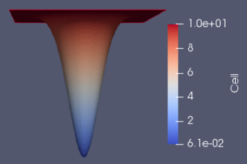
(a) Initial cell density $u_{0}$

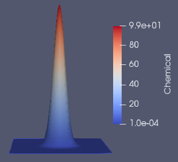
(b) Initial chemical concentration $v_{0}$

Figure 2: Initial conditions.

Note that $u_{0},v_{0}>0$ in $\Omega$, $\min(u_{0})=u_{0}(1,1)=0.0001$ and $\max(v_{0})=v_{0}(1,1)=100.0001$. We obtain that:

1. All the schemes take negative values for the minimum of $u^{n}$ in different times $t_{n}\geq 0$, for the different values considered for $p$ and $\varepsilon$. However, in the case of the schemes UV$\varepsilon$ and US$\varepsilon$, it is observed that these values are closer to $0$ as $\varepsilon\rightarrow 0$ (see Figures 3-9).

2. In all cases, the scheme UV$\varepsilon$ “preserves” better the positivity than the schemes UV, US$\varepsilon$ and US0 (see Figures 3-9).

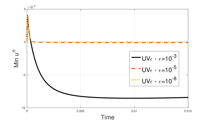
Figure 3: Minimum values of $u^{n}_{\varepsilon}$ for $p=1.1$, computed using the scheme UV$\varepsilon$. We also obtain negative values for $\varepsilon=10^{-8}$ of order $10^{-8}$.

Figure 4: Minimum values of $u^{n}_{\varepsilon}$ for $p=1.1$, computed using the scheme US$\varepsilon$.

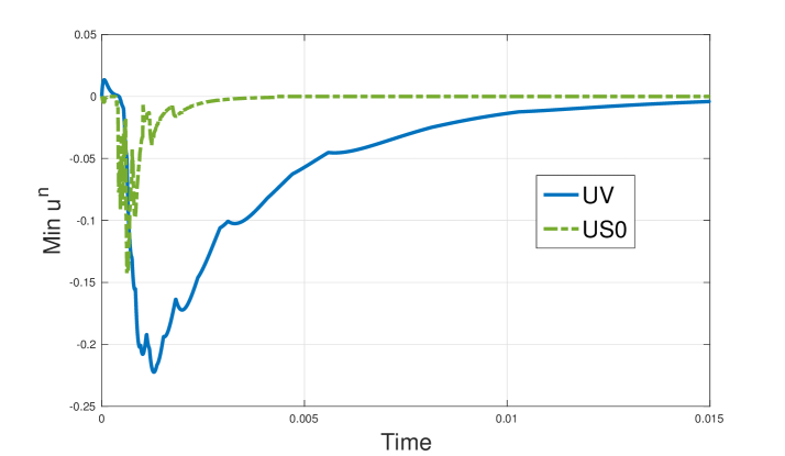
Figure 5: Minimum values of $u^{n}_{\varepsilon}$ for $p=1.1$, computed using the schemes UV and US0.

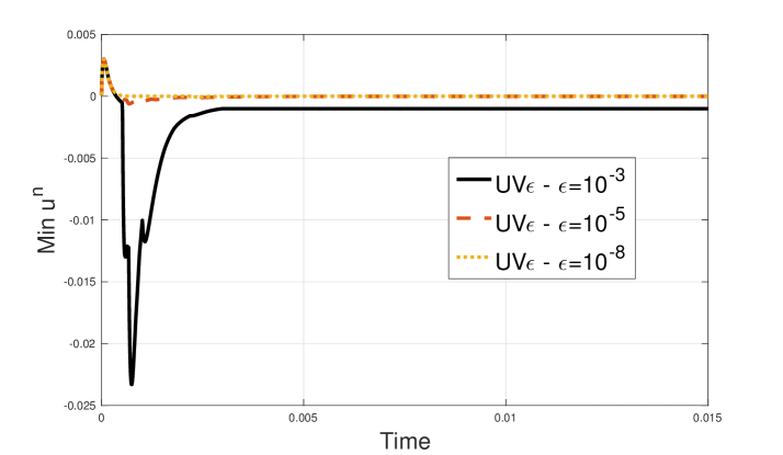
Figure 6: Minimum values of $u^{n}_{\varepsilon}$ for $p=1.5$, computed using the scheme UV$\varepsilon$. We also obtain negative values for $\varepsilon=10^{-8}$ of order $10^{-5}$.

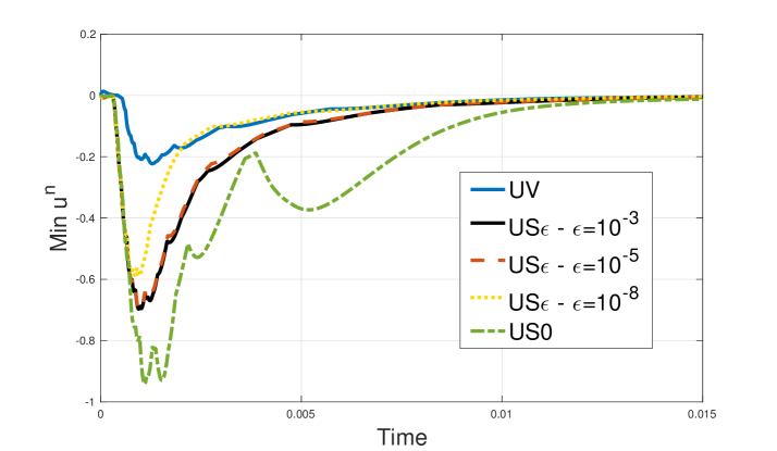
Figure 7: Minimum values of $u^{n}$ for $p=1.5$, computed using the schemes UV, US$\varepsilon$ and US0.

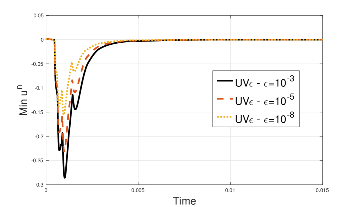
Figure 8: Minimum values of $u^{n}_{\varepsilon}$ for $p=1.9$, computed using the scheme UV$\varepsilon$.

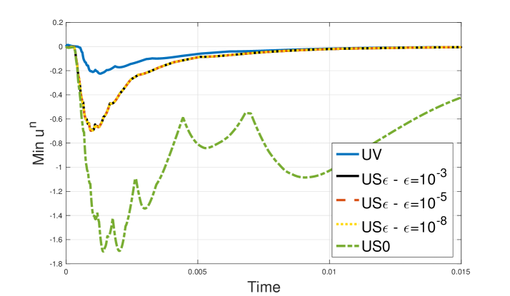
Figure 9: Minimum values of $u^{n}$ for $p=1.9$, computed using the schemes UV, US$\varepsilon$ and US0.

5.2 Energy stability

In this subsection, we compare numerically the stability of the schemes UV$\varepsilon$, US$\varepsilon$, US0 and UV with respect to the “exact” energy

$$\mathcal{E}_{e}(u,v)=\displaystyle\int_{\Omega}\frac{1}{p-1}(u_{+})^{p}d\textit{{x}}+\frac{1}{2}\|\nabla{v}\|_{0}^{2}.$$ (97)

It was proved that the schemes UV$\varepsilon$, US$\varepsilon$ and US0 are unconditionally energy-stables with respect to modified energies defined in terms of the variables of each scheme, and some energy inequalities are satisfied (see Theorems 4.9, 4.17 and 4.24). However, it is not clear how to prove the energy-stability of these schemes with respect to the “exact” energy $\mathcal{E}_{e}(u,v)$ given in (97), which comes from the continuous problem (2) (see (9)-(10)). Therefore, it is interesting to compare numerically the schemes with respect to this energy $\mathcal{E}_{e}(u,v)$, and to study the behavior of the corresponding discrete energy law residual

$$RE_{e}(u^{n},v^{n}):=\delta_{t}\mathcal{E}_{e}(u^{n},v^{n})+\frac{4}{p}\int_{\Omega}|\nabla((u^{n}_{+})^{p/2})|^{2}d\textit{{x}}+\|\Delta_{h}v^{n}\|_{0}^{2}+\|\nabla v^{n}\|_{0}^{2}.$$ (98)

We consider $k=10^{-5}$, $h=\frac{1}{25}$, $p=1.4$, $tol=10^{-3}$ and the initial conditions (see Figure 10)

$$u_{0}=14cos(2\pi x)cos(2\pi y)+14.0001\ \ \mbox{and}\ \ v_{0}=-14cos(2\pi x)cos(2\pi y)+14.0001.$$

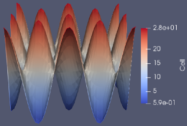
(a) Initial cell density $u_{0}$

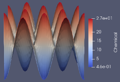
(b) Initial chemical concentration $v_{0}$

Figure 10: Initial conditions.

We choose the space for $v$ generated by $\mathbb{P}_{1}$-continuous FE. Then, we obtain that:

1. All the schemes UV$\varepsilon$, US$\varepsilon$, UV and US0 satisfy the energy decreasing in time property for the exact energy $\mathcal{E}_{e}(u,v)$ (see Figure 11), that is,

   $$\mathcal{E}_{e}(u^{n},v^{n})\leq\mathcal{E}_{e}(u^{n-1},v^{n-1})\ \ \forall n.$$

2. The schemes US0 and US$\varepsilon$ satisfy the discrete energy inequality $RE_{e}(u^{n},v^{n})\leq 0$, for $RE_{e}(u^{n},v^{n})$ defined in (98), independently of the choice of $\varepsilon$; while the schemes UV and UV$\varepsilon$ have $RE(u^{n},v^{n})>0$ for some $t_{n}\geq 0$. However, it is observed that the scheme UV$\varepsilon$ introduces lower numerical source than the scheme UV, and lower numerical dissipation than the schemes US0 and US$\varepsilon$ (see Figure 12).

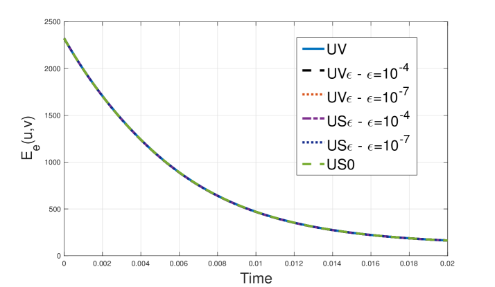
Figure 11: $\mathcal{E}_{e}(u^{n},v^{n})$ of the schemes UV, US0, UV$\varepsilon$ and US$\varepsilon$ (for $\varepsilon=10^{-4},10^{-7}$).

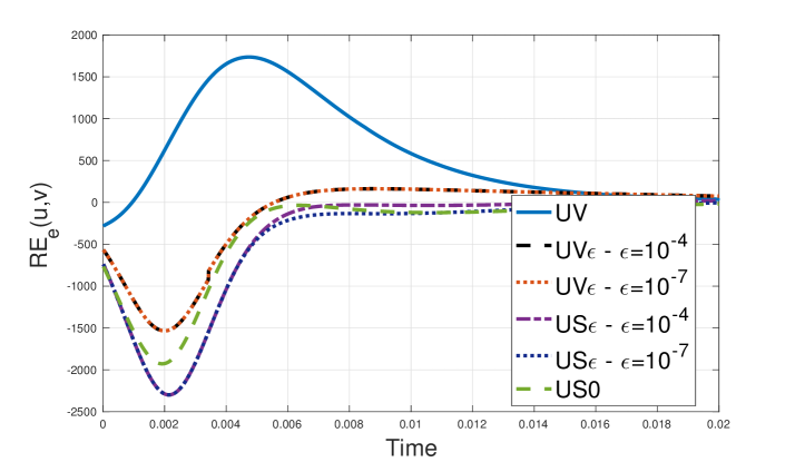
Figure 12: $RE_{e}(u^{n},v^{n})$ of the schemes UV, US0, UV$\varepsilon$ and US$\varepsilon$ (for $\varepsilon=10^{-4},10^{-7}$).

6 Conclusions

In this paper we have developed three new mass-conservative and unconditionally energy-stable fully discrete FE schemes for the chemorepulsion production model (2), namely UV$\varepsilon$, US$\varepsilon$ and US0. From the theoretical point of view we have obtained:

1. The solvability of the numerical schemes.

2. The schemes UV$\varepsilon$ and US$\varepsilon$ are unconditionally energy-stables with respect to the modified energies $\mathcal{E}^{h}_{\varepsilon}(u,v)$ (given in (67)) and $\mathcal{E}^{h}_{\varepsilon}(u,{\boldsymbol{\sigma}})$ (given in (81)) respectively, under the right-angles constraint (H); while the scheme US0 is unconditionally energy-stable with respect to the modified energy $\mathcal{E}^{h}(u,{\boldsymbol{\sigma}})$ given in (90), without this restriction (H) on the mesh.

3. It is not clear how to prove the energy-stability of the nonlinear scheme UV (see Remark 5.1).

4. In the schemes UV$\varepsilon$ and US$\varepsilon$ there is a control for $\Pi^{h}(u^{n}_{\varepsilon-})$ in $L^{2}$-norm, which tends to $0$ as $\varepsilon\rightarrow 0$. This allows to conclude the nonnegativity of the solution $u^{n}_{\varepsilon}$ in the limit as $\varepsilon\rightarrow 0$.

On the other hand, from the numerical simulations, we can conclude:

1. The four schemes have decreasing in time energy $\mathcal{E}_{e}(u,v)$, independently of the choice of $\varepsilon$.

2. The schemes US0 and US$\varepsilon$ satisfy the discrete energy inequality $RE_{e}(u^{n},v^{n})\leq 0$, for $RE_{e}(u^{n},v^{n})$ defined in (98), independently of the choice of $\varepsilon$; while the schemes UV and UV$\varepsilon$ have $RE(u^{n},v^{n})>0$ for some $t_{n}\geq 0$. However, it was observed that the scheme UV$\varepsilon$ introduces lower numerical source than the scheme UV, and lower numerical dissipation than the schemes US0 and US$\varepsilon$.

3. Finally, it was observed numerically that for the schemes UV$\varepsilon$ and US$\varepsilon$, $\underset{\overline{\Omega}\times[0,T]}{\min}\ u^{n}_{\varepsilon}\rightarrow 0$ as $\varepsilon\rightarrow 0$.

References

- [1] G. Allaire, Numerical analysis and optimization. An introduction to mathematical modelling and numerical simulation. Translated from the French by Alan Craig. Numerical Mathematics and Scientific Computation. Oxford University Press, Oxford (2007).
- [2] C. Amrouche and N.E.H. Seloula, -theory for vector potentials and Sobolev’s inequalities for vector fields: application to the Stokes equations with pressure boundary conditions. Math. Models Methods Appl. Sci. 23 (2013), no. 1, 37–92.
- [3] J. Barrett and J. Blowey, Finite element approximation of a nonlinear cross-diffusion population model. Numer. Math. 98 (2004), no. 2, 195–221.
- [4] J. Barrett and R. Nürnberg, Finite-element approximation of a nonlinear degenerate parabolic system describing bacterial pattern formation. Interfaces and Free Boundaries 4 (2002), no. 3, 277–307.
- [5] R. Becker, X. Feng and A. Prohl, Finite element approximations of the Ericksen-Leslie model for nematic liquid crystal flow. SIAM J. Numer. Anal. 46 (2008), 1704–1731.
- [6] M. Bessemoulin-Chatard and A. Jüngel, A finite volume scheme for a Keller-Segel model with additional cross-diffusion. IMA J. Numer. Anal. 34 (2014), no. 1, 96–122.
- [7] T. Cieslak, P. Laurençot and C. Morales-Rodrigo, Global existence and convergence to steady states in a chemorepulsion system. Parabolic and Navier-Stokes equations. Part 1, 105-117, Banach Center Publ., 81, Part 1, Polish Acad. Sci. Inst. Math., Warsaw, 2008.
- [8] Y. Epshteyn and A. Izmirlioglu, Fully discrete analysis of a discontinuous finite element method for the Keller-Segel chemotaxis model. J. Sci. Comput. 40 (2009), no. 1-3, 211–256.
- [9] F. Filbet, A finite volume scheme for the Patlak-Keller-Segel chemotaxis model. Numer. Math. 104 (2006), no. 4, 457–488.
- [10] E. Feireisl and A. Novotný, Singular limits in thermodynamics of viscous fluids. Advances in Mathematical Fluid Mechanics. Birkhäuser Verlag, Basel (2009).
- [11] P. Grisvard, Elliptic Problems in Nonsmooth Domains. Pitman Advanced Publishing Program, Boston (1985).
- [12] G. Grün and M. Rumpf, Nonnegativity preserving convergent schemes for the thin film equation. Numer. Math. 87 (2000), 113–152.
- [13] F. Guillén-González, M.A. Rodríguez-Bellido and D.A. Rueda-Gómez, Study of a chemo-repulsion model with quadratic production. Part I: Analysis of the continuous problem and time-discrete numerical schemes. (Submitted), arXiv:1803.02386 [math.NA].
- [14] F. Guillén-González, M.A. Rodríguez-Bellido and D.A. Rueda-Gómez, Study of a chemo-repulsion model with quadratic production. Part II: Analysis of an unconditional energy-stable fully discrete scheme. (Submitted), arXiv:1803.02391 [math.NA].
- [15] F. Guillén-González, M.A. Rodríguez-Bellido and D.A. Rueda-Gómez, Unconditionally energy stable fully discrete schemes for a chemo-repulsion model. (Submitted), arXiv:1807.01118 [math.NA].
- [16] Y. He and K. Li, Asymptotic behavior and time discretization analysis for the non-stationary Navier-Stokes problem. Numer. Math. 98 (2004), no. 4, 647–673.
- [17] J.L. Lions and E. Magenes, Problèmes aux limites non homogènes et applications, Vol. 1. Travaux et Recherches Mathématiques, No. 17 Dunod, Paris (1968).
- [18] A. Marrocco, Numerical simulation of chemotactic bacteria aggregation via mixed finite elements. M2AN Math. Model. Numer. Anal. 37 (2003), no. 4, 617–630.
- [19] J. Necas, Les Méthodes Directes en Théorie des Equations Elliptiques. Editeurs Academia, Prague (1967).
- [20] N. Saito, Conservative upwind finite-element method for a simplified Keller-Segel system modelling chemotaxis. IMA J. Numer. Anal. 27 (2007), no. 2, 332–365.
- [21] N. Saito, Error analysis of a conservative finite-element approximation for the Keller-Segel system of chemotaxis. Commun. Pure Appl. Anal. 11 (2012), no. 1, 339–364.
- [22] J. Simon, Compact sets in the space . Ann. Mat. Pura Appl. 146 (1987), no. 4, 65–96.
- [23] J. Zhang, J. Zhu and R. Zhang, Characteristic splitting mixed finite element analysis of Keller-Segel chemotaxis models. Appl. Math. Comput. 278 (2016), 33–44.