Maximizing Invariant Data Perturbation with Stochastic Optimization

Abstract

Feature attribution methods, or saliency maps, are one of the most popular approaches for explaining the decisions of complex machine learning models such as deep neural networks. In this study, we propose a stochastic optimization approach for the perturbation-based feature attribution method. While the original optimization problem of the perturbation-based feature attribution is difficult to solve because of the complex constraints, we propose to reformulate the problem as the maximization of a differentiable function, which can be solved using gradient-based algorithms. In particular, stochastic optimization is well-suited for the proposed reformulation, and we can solve the problem using popular algorithms such as SGD, RMSProp, and Adam. The experiment on the image classification with VGG16 shows that the proposed method could identify relevant parts of the images effectively.

1 Introduction

Feature attribution methods [1, 2, 3, 4, 5, 6, 7], or saliency maps, are one of the most popular approaches for explaining the decisions of complex machine learning models such as deep neural networks. In feature attribution, for each of given instance, they score how much each feature is relevant to the model’s decision: they score the features relevant to the model’s decision with large values and irrelevant features with small values. For example, in image recognition, they highlight which pixels the models have focused on by scoring the relevance of each pixel [1, 2, 3, 4, 5], and in text classification, they detect a set of words or sentences relevant to the model’s decision by scoring each words or sentences [8, 9]. With feature attribution methods, one can obtain relevant features, such as pixels or words, as explanations why the models made certain decisions, which also helps the users to inspect whether the models are reliable or not. Major approaches for feature attribution are based on modified gradients [1, 2, 3, 4, 5, 6] and feature maskings [10].

Recently, Hara et al. [7] proposed to separate the definition of the feature attribution scores and the algorithms to compute them. In most of the previous studies, scores are defined by their computation algorithms themselves except for some axiomatic approaches [4, 11]. The separation of the definitions and the algorithms allows us to consider each aspect independently. For example, if the definition is not appropriate, improving algorithms does not help and we need to reconsider the definition in such a situation.

As one possible definition of the feature attribution score, Hara et al. [7] proposed to measure the irrelevance of each feature to the model’s decision by the maximum size of data perturbations that does not change the decision. Specifically, they defined the score as a solution to the optimization problem that maximizes the size of data perturbation under the constraint that the perturbed data to remain inside the model’s decision boundary. They then proposed an algorithm that solves the optimization problem approximately: they approximated the constraint with linear functions and reformulated the problem as linear programming. The linear programming formulation is found to be useful with several flexible extensions such as relaxing constraints and sharing scores among features. The drawback of the linear approximation, however, is that we cannot strictly enforce the perturbed data to stay inside the model’s decision boundary. Therefore, the solution to the linear programming can violate the definition.

This study is positioned as the improvements of the algorithm for the score defined by Hara et al. [7]. Specifically, to relieve the risk of the definition violation in the method of Hara et al. [7], we propose an algorithm to solve the problem without linear approximation. In the proposed approach, we reformulate the problem so that it can be solved by using gradient-based algorithms. Specifically, we rewrite the constraint as a differential penalty function in the objective function to be maximized. With this reformulation, the problem is expressed as the maximization of a differentiable function, which can be solved using gradient-based algorithms. In particular, stochastic optimization is well-suited for the proposed reformulation, and we can solve the problem using popular algorithms such as SGD, RMSProp [12], and Adam [13].

Settings

In this paper, we consider the classification model $f$ for $k$ categories that returns an output $y\in\mathbb{R}^{k}$ for a given input $x\in\mathbb{R}^{d}$, i.e., $y=f(x)$. The classification result is determined as $c=\operatorname*{argmax}_{j}y_{j}$ where $y_{j}=f_{j}(x)$ is the $j$-th element of the output. We assume that the model $f$ is differentiable with respect to the input $x$: the target models therefore include linear models, kernel models with differentiable kernels, and deep neural networks. We assume that the model $f$ and the target input $x$ to be explained are given and fixed.

2 Problem Definition: Maximizing Invariant Data Perturbation

In this section, we briefly review the definition of the problem introduced by Hara et al. [7]. As an explanation of the input $x$, we seek the maximally invariant data perturbation that does not change the model’s decision.

We start from introducing invariant perturbation set. We say that a set $R\subseteq\mathbb{R}^{d}$ is an invariant perturbation set if the model’s decision is invariant for all $r\in R$, i.e., $c=\operatorname*{argmax}_{j}f_{j}(x+r)$.

In the study, for ease of computation, we restrict our attention to a box-shaped invariant perturbation set $R(w)=[-w_{1},w_{1}]\times[-w_{2},w_{2}]\times\cdots\times[-w_{d},w_{d}]$ for a parameter $w\in\mathbb{R}^{d}_{+}$. From this definition of $R(w)$, the size of the invariant perturbation of each feature $x_{i}$ is proportional to $w_{i}$. The idea here is that, if the invariant perturbation $w_{i}$ is small, the change of the feature $x_{i}$ can highly impacts the model’s decision, which indicates that the feature $x_{i}$ is relevant to the decision. On the other hand, if $w_{i^{\prime}}$ is large, the feature $x_{i^{\prime}}$ only has a minor impact to the model’s decision, and thus it is less relevant.

To obtain an invariant perturbation set $R(w)$ appropriate for feature attribution, Hara et al. [7] proposed to maximize the side lengths of the $R(w)$ so that $w_{i}$ to be sufficiently large for irrelevant features.

Problem 2.1 (Maximal Invariant Perturbation).

Find the invariant perturbation set $R(\hat{w})$, where

$$\hat{w}=\operatorname*{argmax}_{w\in\mathbb{R}_{+}^{d},\|w\|_{\infty}\leq C}\sum_{i=1}^{d}w_{i},\;{\rm s.t.}\;c=\operatorname*{argmax}_{j}f_{j}(x+r),\forall r\in R(w).$$ (2.1)

Here, $C>0$ is the upper bound of the perturbation. The value of $C$ can be usually determined from the nature of the data. For example, if the data is the image, the value of each pixel is usually restricted in $[0,1]$. In this case, the upper bound $C=1$ is the natural choice.

3 Proposed Method

We now turn to our proposed method to solve the problem (2.1). The difficulty on solving the problem (2.1) is that it requires the constraint $c=\operatorname*{argmax}_{j}f_{j}(x+r)$ to hold for all possible $r\in R(w)$. In the proposed method, we rewrite the constraint by using the expectation over $r\in R(w)$. In this way, we can reformulate the problem as the maximization of a differentiable function, which can be solved using gradient-based algorithms.

3.1 Problem Reformulation

We reformulate the problem (2.1) into the penalty-based expression, so that the gradient-based optimization algorithms to be applicable. Recall that the constraint $c=\operatorname*{argmax}_{j}f_{j}(x+r)$ is equivalent to a set of constraints $f_{c}(x+r)\geq f_{j}(x+r)$ over $\forall j\neq c$. Here, we rewrite the constraint $f_{c}(x+r)\geq f_{j}(x+r)$ into the following equivalent expression using expectation.

Proposition 3.1.

The constraint $f_{c}(x+r)\geq f_{j}(x+r),\forall r\in R(w)$ is equivalent to

$$\mathbb{E}_{t}[\max\{0,f_{j}(x+t\odot w)-f_{c}(x+t\odot w)\}]\leq 0,$$ (3.1)

where $\mathbb{E}_{t}$ denotes the expectation over uniformly random $t\in[-1,1]^{d}$, and $\odot$ denotes an element-wise product.

Proof.

We first note that $r:=t\odot w$ is a uniform random variable in $R(w)$. Here, recall that $\max\{0,f_{j}(x+r)-f_{c}(x+r)\}$ is non-negative. Therefore, the inequality $\max\{0,f_{j}(x+r)-f_{c}(x+r)\}\leq 0$ holds if and only if $f_{c}(x+r)\geq f_{j}(x+r)$. Hence, for the inequality $\mathbb{E}_{t}[\max\{0,f_{j}(x+r)-f_{c}(x+r)\}]\leq 0$ to hold, the measure of the points that violates the inequality, i.e., $\{r\in R(w):f_{c}(x+r)<f_{j}(x+r)\}$, must be zero. ∎

We now put the constraint (3.1) as a penalty term in the objective function of (2.1):

$$\begin{split}\hat{w}=&\operatorname*{argmax}_{w\in\mathbb{R}_{+}^{d}}\sum_{i=1}^{d}w_{i}-\lambda\sum_{j\neq c}\mathbb{E}_{t}[h_{jc}(x+t\odot w)],\end{split}$$ (3.2)

where $\lambda\geq 0$ is a penalty parameter, and $h_{jc}(x+t\odot w):=\max\{0,f_{j}(x+t\odot w)-f_{c}(x+t\odot w)\}$. We note that, in the problem (3.2), the constraint (3.1) holds for sufficiently large $\lambda$, and hence the problem (3.2) is equivalent to (2.1).

3.2 Stochastic Optimization

Thanks to the formulation (3.2), it is differentiable with respect to the parameter $w$. Hence, we can apply the gradient-based optimization methods. Here, we note that stochastic optimization algorithms, such as SGD, RMSProp [12], and Adam [13], are particularity suited for the problem. In each iteration of the algorithm, we randomly generate perturbations $\{t_{m}:t_{m}\sim\mathrm{Uniform}([-1,1]^{d})\}_{m=1}^{M}$, and approximate the objective function using the sample average:

$$\sum_{i=1}^{d}w_{i}-\lambda\sum_{j\neq c}\frac{1}{M}\sum_{m=1}^{M}h_{jc}(x+t_{m}\odot w).$$ (3.3)

The psuedo code of the stochastic optimization is shown in Algorithm 1. The line 6 is added in the algorithm so that the parameter $w$ to stay between the lower bound zero and the upper bound $C$.

1:Initialize $w$ with a zero vector

2:while not converged do

3:     Sample $\{t_{m}:t_{m}\sim\mathrm{Uniform}([-1,1]^{d})\}_{m=1}^{M}$

4:     Compute the gradient of (3.3)

5:     Update $w$ using an update rule, such as SGD, RMSProp, and Adam

6:     Clip $w$ as $w=\min\{\max\{0,w\},C\}$

7:end while

8:Return $w$

Algorithm 1 Stochastic Optimization

4 Experiment

4.1 Experimental Setup

In the experiment, we followed the setup used in Hara et al. [7]. As the target model $f$ to be explained, we adopted the pre-trained VGG16 [14] distributed at the Tensorflow repository. As the target data $x$ to be explained, we used COCO-animal dataset. Specifically, for the experiment, we used $200$ images in the validation set.

In the proposed method, we set $\lambda=0.1d$ and $M=32$ where the data dimension is $d=224\times 224\times 3$ . As the optimization algorithm, we used Adam [13] with the step size set to $0.01$ and remaining parameters set to be default values. To measure the relevance of the feature $x_{i}$ to the model’s decision, we used $-\hat{w}_{i}$, the negative of the perturbation size, as the score. Large score, or small $\hat{w}_{i}$, means that the change of the feature $x_{i}$ can highly impacts the model’s decision, which indicates that the feature $x_{i}$ is relevant to the decision. On the other hand, if the score is small, or $w_{i^{\prime}}$ is large, the feature $x_{i^{\prime}}$ only has a minor impact to the model’s decision, and thus it is less relevant.

As the baseline methods, we used Gradient [1], GuidedBP [2], SmoothGrad [5], IntGrad [4], LRP [3], DeepLIFT [6], Occlusion, and the LP-based methods (LP and LP(Smooth)) [7]. Gradient, GuidedBP, SmoothGrad and IntGrad are implemented using saliency with default settings, and LRP, DeepLIFT, and Occlusion are implemented using DeepExplain where we set the mask size for Occlusion as $(12,12,3)$. For the LP-based methods, we used the same setting as the ones used in Hara et al. [7] ($\delta=0.1$ and $\lambda\approx 0.5$). We note that, all the methods including the proposed method return the scores of size $(224,224,3)$.

4.2 Result

We evaluated the effectiveness of each method by making pixels of the images. Specifically, we mask low score pixels with gray colors and observe whether the model’s classification result is resistant to the flipping. We expect that good feature attribution methods to identify relevant pixels with high scores. Therefore, with good attribution methods, the model’s classification result will kept unchanged even if we flip many low score pixels to gray, as relevant parts of the images remain unflipped. On the other hand, if the attribution methods fail to identify relevant pixels with high scores, the classification result can change even with a small number of flips.

We conducted the experiment as follows.

1. Flip pixels with scores smaller than the $\tau$% quantile to $0.5$ (i.e., we replace the selected pixels with gray pixels).

2. Observe the ratio of the images with the classification result changes within the 200 images: the result changes in less images indicate that the feature attribution methods successfully identified relevant parts of the images.

We varied the threshold quantile from $\tau=0$ (no flip) to $\tau=100$ (all filp), and summarized the result in Figure 1. It is clear that the proposed method is the most resistant to the masking: the changes on the classification results are kept almost zeros even if 50% of the pixels are masked. This indicates that the proposed method successfully identified relevant parts of the images. Moreover, the proposed method consistently outperformed the LP-based methods. We conjecture that the LP-based methods can violate the constraint in the problem because of approximation, which led to less accurate estimate of the solution to the problem (2.1). By contrast, the proposed method solves the problem without approximation. Hence, the derived solution is more accurate than the ones of the LP-based methods.

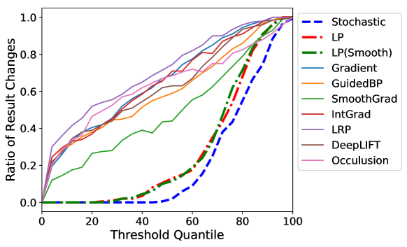
Figure 1: The ratio of the classification result changes when high score image patches are flipped to gray. Stochastic denotes the proposed method.

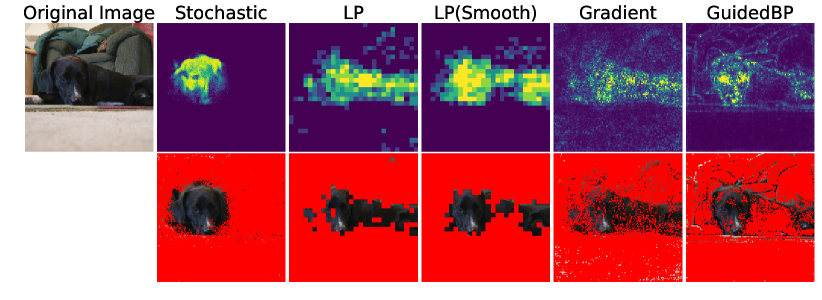
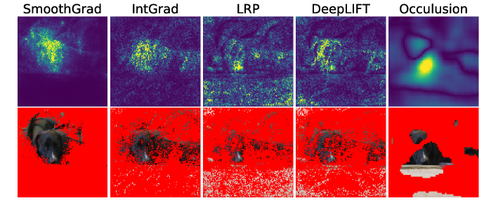
Figure 2: Example images (dog): the computed scores as heatmap (top); the filtered images with pixels with scores lower than the 80% quantiles are filtered out with red (bottom). Stochastic denotes the proposed method.

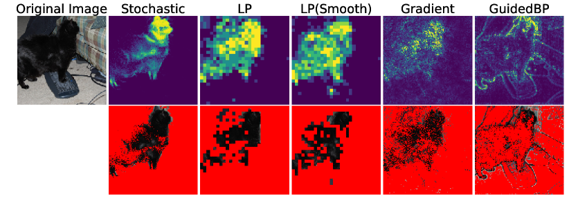
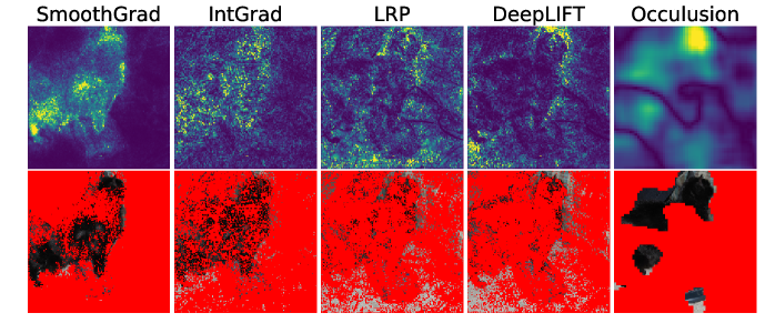
Figure 3: Example images (cat): the computed scores as heatmap (top); the filtered images with pixels with scores lower than the 80% quantiles are filtered out with red (bottom). Stochastic denotes the proposed method.

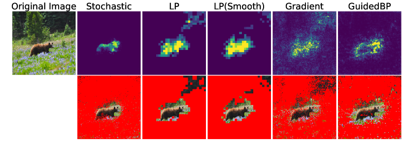
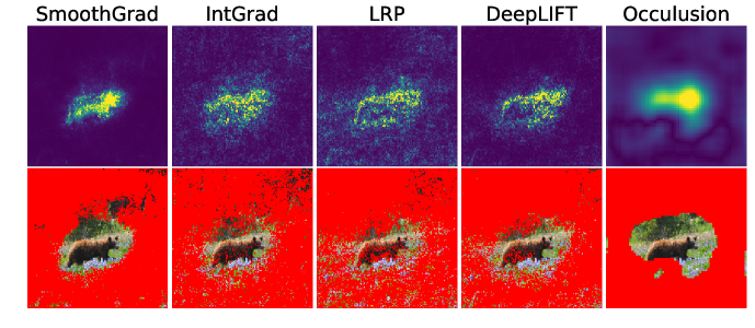
Figure 4: Example images (bear): the computed scores as heatmap (top); the filtered images with pixels with scores lower than the 80% quantiles are filtered out with red (bottom). Stochastic denotes the proposed method.

Figures 2, 3, and 4 show examples of the computed scores with each feature attirbution method. The figures clearly show that the proposed method attained a very high S/N ratios compared to the existing method where the scores tend to be noisy. We conjecture that this was because the proposed method could provide high quality solutions to the problem (2.1) without linear approximation.

5 Conclusion

In this study, as a novel feature attribution method, we proposed a stochastic optimization method for finding maximally invariant data perturbation. In the proposed approach, we reformulated the problem as the maximization of a differentiable function, which can be solved using gradient-based algorithms. In particular, stochastic optimization is well-suited for the proposed reformulation, and we can solve the problem using popular algorithms such as SGD, RMSProp, and Adam. The experimental result on the image classification with VGG16 shows that the proposed method could identify relevant parts of the images effectively.

References

- [1] Karen Simonyan, Andrea Vedaldi, and Andrew Zisserman. Deep inside convolutional networks: Visualising image classification models and saliency maps. arXiv:1312.6034, 2013.
- [2] Jost Tobias Springenberg, Alexey Dosovitskiy, Thomas Brox, and Martin Riedmiller. Striving for simplicity: The all convolutional net. arXiv:1412.6806, 2014.
- [3] Sebastian Bach, Alexander Binder, Grégoire Montavon, Frederick Klauschen, Klaus-Robert Müller, and Wojciech Samek. On pixel-wise explanations for non-linear classifier decisions by layer-wise relevance propagation. PloS ONE, 10(7):e0130140, 2015.
- [4] Mukund Sundararajan, Ankur Taly, and Qiqi Yan. Axiomatic attribution for deep networks. arXiv:1703.01365, 2017.
- [5] Daniel Smilkov, Nikhil Thorat, Been Kim, Fernanda Viégas, and Martin Wattenberg. Smoothgrad: removing noise by adding noise. arXiv:1706.03825, 2017.
- [6] Avanti Shrikumar, Peyton Greenside, and Anshul Kundaje. Learning important features through propagating activation differences. In Proceedings of International Conference on Machine Learning, pages 3145–3153, 2017.
- [7] Satoshi Hara, Kouichi Ikeno, Tasuku Soma, and Takanori Maehara. Maximally invariant data perturbation as explanation. arXiv:1806.07004, 2018.
- [8] Yanzhuo Ding, Yang Liu, Huanbo Luan, and Maosong Sun. Visualizing and understanding neural machine translation. Proceedings of the 55th Annual Meeting of the Association for Computational Linguistics, pages 1150–1159, 2017.
- [9] Jianbo Chen, Le Song, Martin Wainwright, and Michael Jordan. Learning to explain: An information-theoretic perspective on model interpretation. In Proceedings of the 35th International Conference on Machine Learning, pages 882–891, 2018.
- [10] Ruth C Fong and Andrea Vedaldi. Interpretable explanations of black boxes by meaningful perturbation. In Proceeding of the IEEE International Conference on Computer Vision, pages 3449 – 3457, 2017.
- [11] Scott M Lundberg and Su-In Lee. A unified approach to interpreting model predictions. In Proceedings of Advances in Neural Information Processing Systems, pages 4765–4774, 2017.
- [12] Tijmen Tieleman and Geoffrey Hinton. Lecture 6.5-rmsprop: Divide the gradient by a running average of its recent magnitude. COURSERA: Neural networks for machine learning, 4(2):26–31, 2012.
- [13] Diederik P Kingma and Jimmy Ba. Adam: A method for stochastic optimization. arXiv:1412.6980, 2014.
- [14] Karen Simonyan and Andrew Zisserman. Very deep convolutional networks for large-scale image recognition. arXiv:1409.1556, 2014.