Push-Down Trees: Optimal Self-Adjusting Complete Trees

Abstract

This paper studies a fundamental algorithmic problem related to the design of demand-aware networks: networks whose topologies adjust toward the traffic patterns they serve, in an online manner. The goal is to strike a tradeoff between the benefits of such adjustments (shorter routes) and their costs (reconfigurations). In particular, we consider the problem of designing a self-adjusting tree network which serves single-source, multi-destination communication. The problem has interesting connections to self-adjusting datastructures. We present two constant-competitive online algorithms for this problem, one randomized and one deterministic. Our approach is based on a natural notion of Most Recently Used (MRU) tree, maintaining a working set. We prove that the working set is a cost lower bound for any online algorithm, and then present a randomized algorithm Random-Push which approximates such an MRU tree at low cost, by pushing less recently used communication partners down the tree, along a random walk. Our deterministic algorithm Move-Half  does not directly maintain an MRU tree, but its cost is still proportional to the cost of an MRU tree, and also matches the working set lower bound.

1 Introduction

While datacenter networks traditionally rely on a fixed topology, recent optical technologies enable reconfigurable topologies which can adjust to the demand (i.e., traffic pattern) they serve in an online manner, e.g. [20, 25, 22, 10]. Indeed, the physical topology is emerging as the next frontier in an ongoing effort to render networked systems more flexible.

In principle, such topological reconfigurations can be used to provide shorter routes between frequently communicating nodes, exploiting structure in traffic patterns [5, 24, 25], and hence to improve performance. However, the design of self-adjusting networks which dynamically optimize themselves toward the demand introduces an algorithmic challenge: an online algorithm needs to be devised which guarantees an efficient tradeoff between the benefits (i.e., shorter route lengths) and costs (in terms of reconfigurations) of topological optimizations.

This paper focuses on the design of a self-adjusting complete tree ($\mathrm{CT}$) network: a network of nodes (e.g., servers or racks) that forms a complete tree, and we measure the routing cost in terms of the length of the shortest path between two nodes. Trees are not only a most fundamental topological structure of their own merit, but also a crucial building block for more general self-adjusting network designs: Avin et al. [6, 7] recently showed that multiple tree networks (optimized individually for a single source node) can be combined to build general networks which provide low degree and low distortion. The design of a dynamic single-source multi-destination communication tree, as studied in this paper, is hence a stepping stone.

The focus on trees is further motivated by a relationship of our problem to problems arising in self-adjusting datastructures [8]: self-adjusting datastructures such as self-adjusting search trees [31] have the appealing property that they optimize themselves to the workload, leveraging temporal locality, but without knowing the future. Ideally, self-adjusting datastructures store items which will be accessed (frequently) in the future, in a way that they can be accessed quickly (e.g., close to the root, in case of a binary search tree), while also accounting for reconfiguration costs. However, in contrast to most datastructures, in a network, the search property is not required: the network supports routing. Accordingly our model can be seen as a novel flavor of such self-adjusting binary search trees where lookup is supported by a map, enabling shortest path routing (more details will follow).

We present a formal model for this problem later, but a few observations are easy to make. If we restrict ourselves to the special case of a line network (a “linear tree”), the problem of optimally arranging the destinations of a given single communication source is equivalent to the well-known dynamic list update problem: for such self-adjusting (unordered) lists, dynamically optimal online algorithms have been known for a long time [30]. In particular, the simple move-to-front algorithm which immediately promotes the accessed item to the front of the list, fulfills the Most-Recently Used (MRU) property: the $i^{\mathit{th}}$ furthest away item from the front of the list is the $i^{\mathit{th}}$ most recently used item. In the list (and hence on the line), this property is enough to guarantee optimality. The MRU property is related to the so called working set property: the cost of accessing item $x$ at time $t$ depends on the number of distinct items accessed since the last access of $x$ prior to time $t$, including $x$. Naturally, we wonder whether the MRU property is enough to guarantee optimality also in our case. The answer turns out to be non-trivial.

A first contribution of this paper is the observation that if we count only access cost (ignoring any rearrangement cost, see Definition 1 for details), the answer is affirmative: the most-recently used tree is what is called access optimal. Furthermore, we show that the corresponding access cost is a lower bound for any algorithm which is dynamically optimal. But securing this property, i.e., maintaining the most-recently used items close to the root in the tree, introduces a new challenge: how to achieve this at low cost? In particular, assuming that swapping the locations of items comes at a unit cost, can the property be maintained at cost proportional to the access cost? As we show, strictly enforcing the most-recently used property in a tree is too costly to achieve optimality. But, as we will show, when turning to an approximate most-recently used property, we are able to show two important properties: i) such an approximation is good enough to guarantee access optimality; and ii) it can be maintained in expectation using a randomized algorithm: less recently used communication partners are pushed down the tree along a random walk.

While the most-recently used property is sufficient, it is not necessary: we provide a deterministic algorithm which is dynamically optimal but does not even maintain the MRU property approximately. However, its cost is still proportional to the cost of an MRU tree (Definition 4).

Succinctly, we make the following contributions. First we show a working set lower bound for our problem. We do so by proving that an MRU tree is access optimal. In the following theorem, let $WS(\sigma)$ denote the working set of $\sigma$ (a formal definition will follow later).

Theorem 1

Consider a request sequence $\sigma$. Any algorithm Alg serving $\sigma$ using a self-adjusting complete tree, has cost at least $\mathrm{cost}(\textsc{Alg}(\sigma))\geq WS(\sigma)/4$, where $WS(\sigma)$ is the working set of $\sigma$.

Our main contribution is a deterministic online algorithm Move-Half which maintains a constant competitive self-adjusting Complete Tree ($\mathrm{CT}$) network.

Theorem 2

Move-Half algorithm is dynamically optimal.

Interestingly, Move-Half does not require the MRU property and hence does not need to maintain MRU tree. This implies that maintaining a working set on $\mathrm{CT}$s is not a necessary condition for dynamic optimality, although it is a sufficient one.

Furthermore, we present a dynamically optimal, i.e., constant competitive (on expectation) randomized algorithm for self-adjusting $\mathrm{CT}$s called Random-Push. Random-Push relies on maintaining an approximate MRU tree.

Theorem 3

The Random-Push algorithm is dynamically optimal on expectation.

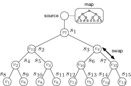
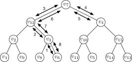
(a)	(b)	(c)

Figure 1: (a) Our complete tree model: a source with a map, a tree of servers that host items (nodes) and a swap operation between neigboring items. (b) The node’s tree network implied by the tree $T$ from (a) and the set of swaps needed to interchange the location of $v_{6}$ and $v_{4}$. (c) The tree network after the interchange and swap operations of (b).

Paper Organization:We discuss problem model and other preliminaries in Section 2 followed by lower bound in Section 3. The deterministic algorithm Move-Half with analysis is provided in Section 4. The randomized algorithm Random-Push is discussed in Section 5. Related work is in Section 6. We conclude in Section 7 followed by an appendix.

2 Model and Preliminaries

Our problem can be formalized using the following simple model. We consider a single source that needs to communicate with a set of $n$ nodes $V=\{v_{1},\ldots,v_{n}\}$. The nodes are arranged in a complete binary tree and the source is connected the the root of the tree. While the tree describes a reconfigurable network, we will use terminology from datastructures, to highlight this relationship and avoid the need to introduce new terms.

We consider a complete tree $T$ connecting $n$ servers $S=\{s_{1},\ldots,s_{n}\}$. We will denote by $s_{1}(T)$ the root of the tree $T$, or $s_{1}$ when $T$ is clear from the context, and by $s_{i}.\mathrm{left}$ (resp. $s_{i}.\mathrm{right}$) the left (resp. right) child of server $s_{i}$. We assume that the $n$ servers store $n$ items (nodes) $V=\{v_{1},\ldots,v_{n}\}$, one item per server. For any $i\in[1,n]$ and any time $t$, we will denote by $s_{i}.\mathrm{guest}^{(t)}\in V$ the item mapped to $s_{i}$ at time $t$. Similarly, $v_{i}.\mathrm{host}^{(t)}\in S$ denotes the server hosting item $v_{i}$. Note that if $v_{i}.\mathrm{host}^{(t)}=s_{j}$ then $s_{j}.\mathrm{guest}^{(t)}=v_{i}$.

The depth of a server $s_{i}$ is fixed and describes the distance from the root; it is denoted by $s_{i}.\mathrm{dep}$, and $s_{1}.\mathrm{dep}=0$. The depth of an item $v_{i}$ at time $t$ is denoted by $v_{i}.\mathrm{dep}^{(t)}$, and is given by the depth of the server to which $v_{i}$ is mapped at time $t$. Note that $v_{i}.\mathrm{dep}^{(t)}=v_{i}.\mathrm{host}.\mathrm{dep}^{(t)}$.

To this end, we interpret communication requests from the source as accesses to items stored in the (unordered) tree. All access requests (resp. communication requests) to items (resp. nodes) originate from the root $s_{1}$. If an item (resp. node) is frequently requested, it can make sense to move this item (node) closer to the root of $T$: this is achieved by swapping items which are neighboring in the tree (resp.  by performing local topological swaps).

Access requests occur over time, forming a (finite or infinite) sequence $\sigma=(\sigma^{(1)},\sigma^{(2)},\ldots)$, where $\sigma^{(t)}=v_{i}\in V$ denotes that item $v_{i}$ is requested, and needs to be accessed at time $t$. The sequence $\sigma$ (henceforth also called the workload) is revealed one-by-one to an online algorithm On. The working set of an item $v_{i}$ at time $t$ is the set of distinct elements accessed since the last access of $v_{i}$ prior to time $t$, including $v_{i}$. We define the rank of item $v_{i}$ at time $t$ to be the size of the working set of $v_{i}$ at time $t$ and denote it as $v_{i}.\mathrm{rank}^{(t)}$. When $t$ is clear of context, we simply write $v_{i}.\mathrm{rank}$. The working set bound of sequence $\sigma$ of $m$ requests is defined as $WS(\sigma)=\sum_{t=1}^{m}\log(\sigma^{(t)}.\mathrm{rank})$.

Both serving (i.e., routing) the request and adjusting the configuration comes at a cost. We will discuss the two cost components in turn. Upon a request, i.e., whenever the source wants to communicate to a partner, it routes to it via the tree $T$. To this end, a message passed between nodes can include, for each node it passes, a bit indicating which child to forward the message next (requires $O(\log n$) bits). Such a source routing header can be built based on a dynamic global map of the tree that is maintained at the source node. As mentioned, the source node is a direct neighbor of the root of the tree, aware of all requests, and therefore it can maintain the map. The access cost is hence given by the distance between the root and the requested item, which is basically the depth of the item in the tree.

The reconfiguration cost is due to the adjustments that an algorithm performs on the tree. We define the unit cost of reconfiguration as a swap: a swap means changing position of an item with its parent. Note that, any two items $u,v$ in the tree can be interchanged using a number of swaps equal to twice the distance between them. This can be achieved by $u$ first swapping along the path to $v$ and then $v$ swapping along the same path to initial location of $u$. This interchange operation results in the tree staying the same, but only $u$ and $v$ changing locations. We assume that to interchange items, we first need to access one of them. See Figure 1 for an example of our model and interchange operation.

Definition 1 (Cost)

The cost incurred by an algorithm Alg to serve a request $\sigma^{(t)}=v_{i}$ is denoted by $\mathrm{cost}(\textsc{Alg}(\sigma^{(t)}))$, short $\mathrm{cost}^{(t)}$. It consists of two parts, access cost, denoted $\mathrm{acc\text{-}}\mathrm{cost}^{(t)}$, and adjustment cost, denoted $\mathrm{adj\text{-}}\mathrm{cost}^{(t)}$. We define access cost simply as $\mathrm{acc\text{-}}\mathrm{cost}^{(t)}=v_{i}.\mathrm{dep}^{(t)}$ since Alg can maintain a global map and access $v_{i}$ via the shortest path. Adjustment cost, $\mathrm{adj\text{-}}\mathrm{cost}^{(t)}$, is the total number of swaps, where a single swap means changing position of an item with its parent or a child. The total cost, incurred by Alg is then

$$\mathrm{cost}(\textsc{Alg}(\sigma))=\sum_{t}\mathrm{cost}(\textsc{Alg}(\sigma^{(t)}))=\sum_{t}\mathrm{cost}^{(t)}=\sum_{t}(\mathrm{acc\text{-}}\mathrm{cost}^{(t)}+\mathrm{adj\text{-}}\mathrm{cost}^{(t)})$$

Our main objective is to design online algorithms that perform almost as well as optimal offline algorithms (which know $\sigma$ ahead of time), even in the worst-case. In other words, we want to devise online algorithms which minimize the competitive ratio:

Definition 2 (Competitive Ratio $\rho$)

We consider the standard definition of (strict) competitive ratio $\rho$, i.e., $\rho=\max_{\sigma}\mathrm{cost}(\textsc{On})/\mathrm{cost}(\textsc{Opt})$ where $\sigma$ is any input sequence and where Opt denotes the optimal offline algorithm.

If an online algorithm is constant competitive, independently of the problem input, it is called dynamically optimal.

Definition 3 (Dynamic Optimality)

An (online) algorithm On achieves dynamic optimality if it asymptotically matches the offline optimum on every access sequence. In other words, the algorithm On is $O(1)$-competitive.

We also consider a weaker form of competitivity (similarly to the notion of search-optimality in related work [9]), and say that On is access-competitive if we consider only the access cost of On (and ignore any adjustment cost) when comparing it to Opt (which needs to pay both for access and adjustment). For a randomized algorithm, we consider an oblivious online adversary which does not know the random bits of the online algorithm a priori.

The Self-adjusting Complete Tree Problem considered in this paper can then be formulated as follows: Find an online algorithm which serves any (finite or infinite) online request sequence $\sigma$ with minimum cost (including both access and rearrangement costs), on a self-adjusting complete binary tree.

3 Access Optimality: A Working Set Lower Bound

For fixed trees, it is easy to see that keeping frequent items close to the root, i.e., using a Most-Frequently Used (MFU) policy, is optimal (cf. Appendix). The design of online algorithms for adjusting trees is more involved. In particular, it is known that MFU is not optimal for lists [30]. A natural strategy could be to try and keep items close to the root which have been frequent “recently”. However, this raises the question over which time interval to compute the frequencies. Moreover, changing from one MFU tree to another one may entail high adjustment costs.

This section introduces a natural pendant to the MFU tree for a dynamic setting: the Most Recently Used (MRU) tree. Intuitively, the MRU tree tries to keep the “working set” resp. recently accessed items close to the root. In this section we show a working set lower bound for any self-adjusting complete binary tree.

While the move-to-front algorithm, known to be dynamically optimal for self-adjusting lists [30], naturally provides such a “most recently used” property, generalizing move-to-front to the tree is non-trivial. We therefore first show that any algorithm that maintains an MRU tree is access-competitive. With this in mind, let us first formally define the MRU tree.

Definition 4 (MRU Tree)

For a given time $t$, a tree $T$ is an MRU tree if and only if,

$$v_{i}.\mathrm{dep}=\lfloor\log v_{i}.\mathrm{rank}\rfloor$$ (1)

Accordingly the root of the tree (level zero) will always host an item of $\mathrm{rank}$ one. More generally, servers in level $i$ will host items that have a $\mathrm{rank}$ between $(2^{i},2^{i+1}-1)$. Upon a request of an item, say $v_{j}$ with $\mathrm{rank}$ $r$, the $\mathrm{rank}$ of $v_{j}$ is updated to one, and only the ranks of items with $\mathrm{rank}$ smaller than $r$ are increased, each by 1. Therefore, the $\mathrm{rank}$ of items with rank higher than $r$ do not change and their level (i.e., depth) in the MRU tree remains the same (but they may switch location within the same level).

Definition 5 (MRU algorithm)

An online algorithm On has the MRU property (or the working set property) if for each time $t$, the tree $T^{(t)}$ that On maintains, is an MRU tree.

The working set lower bound will follow from the following theorem (Theorem 4) which states that any algorithm that has the MRU property is access competitive. Recall that an analogous statement of Theorem 4 is known to be true for a list [30]. As such, one would hope to find a simple proof that holds for complete trees, but it turns out that this is not trivial, since Opt has more freedom in trees. We therefore present a direct proof based on a potential function, similar in spirit to the list case.

Theorem 4

Any online algorithm On that has the MRU property is 4 access-competitive.

Proof: Consider the two algorithms On and Opt. We employ a potential function argument which is based on the difference in the items’ locations between On’s tree and Opt’s tree. For any server $s_{i}$, we define a pair $(s_{i},s_{j})$ as bad on a tree of some algorithm $A$ if $s_{i}.\mathrm{dep}<s_{j}.\mathrm{dep}$ but $s_{i}.\mathrm{guest}.\mathrm{rank}(A)>s_{j}.\mathrm{guest}.\mathrm{rank}(A)$, i.e., $s_{i}$ is at a lower level although $s_{j}.\mathrm{guest}(A)$ has been accessed more recently. We observe that any bad pair $(s_{i},s_{j})$ for $s_{i}$ is an ordered pair, i.e., this pair is not bad for $s_{j}$. Also note that, for any server $s_{i}$, $s_{i}.\mathrm{dep}$ is same on any tree for any algorithm, what may differ is $s_{i}.\mathrm{guest}$ resp. $s_{i}.\mathrm{guest}.\mathrm{rank}$. Since On has the MRU property it follows by definition that none of its pairs are bad. Hence bad pairs appear only on Opt’s tree. Let, for any algorithm $A$, $\alpha_{i}(A)$ denote the number of bad pairs for $s_{i}$ in $A$’s tree. Let $B_{i}(A)$ be equal to one plus $\alpha_{i}(A)$ divided by the number of elements at level $s_{i}.\mathrm{dep}$. More formally, $B_{i}(A)=1+\frac{\alpha_{i}(A)}{2^{s_{i}.\mathrm{dep}}}$. Define $B(A)=\prod_{i=1}^{n}B_{i}(A)$. Now we define the potential function $\Phi=\log B(\textsc{Opt})-\log B(\textsc{On})$ which is based on the difference in the number of bad pairs between On’s tree and Opt’s tree. According to our definition, $B(\textsc{On})=1$ and hence $\Phi=\log B(\textsc{Opt})$. Therefore, from now onwards, we use $B$ resp. $\log B$ instead of $B(\textsc{Opt})$ resp. $\log B(\textsc{Opt})$. We consider the occurrence of events in the following order. Upon a request, On adjusts its tree, then Opt performs the rearrangements it requires.

Let the potential at time $t$ be $\Phi$ (i.e., before On’s adjustment, after serving request $\sigma^{(t)}$, and before Opt’s rearrangements between requests $t$ and $t+1$) and the potential after On adjusted to its tree be $\Phi^{\prime}$. Then the potential change due to On’s adjustment is

$$\Delta\Phi_{1}=\Phi^{\prime}-\Phi=\log B^{\prime}-\log B=\log\frac{B^{\prime}}{B}$$

We assume that the initial potential is $0$ (i.e., no item was accessed). Since the potential is always positive by definition, we can use it to bound the amortized cost of On, $\mathrm{amortized}(\textsc{On})$. Consider a request at time $t$ to an item at depth $k$ in the tree of On. The access-cost is $\mathrm{cost}^{(t)}(\textsc{On})=k$ and we would like to have the following bound: $\mathrm{amortized}^{(t)}(\textsc{On})\leq\mathrm{cost}^{(t)}(\textsc{On})+\Delta\Phi$. Assume that the requested item $\sigma^{(t)}$ is at server $s_{r}$ at depth $j$ in Opt’s tree, so Opt must pay at least an access cost of $j$. Let $k$ be the depth of $\sigma^{(t)}$ in On tree. First we assume that $j<k$.

Let us compute the potential after On updated its MRU tree. For any server $s_{i}$ at depth lower than $j$ i.e., for which $s_{i}.\mathrm{dep}<j$, it holds that $B^{\prime}_{i}=B_{i}+1/2^{s_{i}.\mathrm{dep}}\leq B_{i}+1$: since the rank of the guest of the last accessed server, $s_{r}$, changed (to $1$) and hence $\alpha_{i}$ increases by 1 for all of them. That is, for all servers for which $s_{i}.\mathrm{dep}\geq j$ (excluding $s_{r}$), $B^{\prime}_{i}=B_{i}$. The potential of the accessed server, $s_{r}$, will be $B^{\prime}_{r}=1$, since its guest’s rank becomes $1$. Although due to the access, the rank of some other elements increase by 1, that does not affect the number of bad pairs. Let the rank of the requested element $\sigma^{(t)}$ before it was accessed be $\sigma^{(t)}.\mathrm{rank}$. After the access at time $t$, the rank of all the elements with rank lesser than $\sigma^{(t)}.\mathrm{rank}$ will increase by 1. Consider any pair $(s_{i},s_{j})$ before the access of $\sigma^{(t)}$. We have already seen what happens if either $s_{i}$ or $s_{j}$ is $s_{r}$. Otherwise a pair $(s_{i},s_{j})$ cannot change from bad to good (resp. good to bad) since if only $s_{j}.\mathrm{rank}$ (resp. $s_{i}.\mathrm{rank}$) increases by 1, it cannot be more than that of $s_{i}$ (resp. $s_{j}$). Now:

$$B^{\prime}=\prod_{i=1}^{n}B^{\prime}_{i} \leq\left(\prod_{s_{i}.\mathrm{dep}<j}(B_{i}+1)\right)\left(\prod_{\begin{subarray}{c}s_{i}.\mathrm{dep}\geq j\\ i\neq r\end{subarray}}B_{i}\right)B^{\prime}_{r}$$

$$\leq\left(2^{j}\prod_{s_{i}.\mathrm{dep}<j}B_{i}\right)B_{r}\left(\prod_{\begin{subarray}{c}s_{i}.\mathrm{dep}\geq j\\ i\neq r\end{subarray}}B_{i}\right)\frac{B^{\prime}_{r}}{B_{r}}$$

$$=\frac{2^{j}}{B_{r}}\prod_{i=1}^{n}B_{i}=\frac{2^{j}}{B_{r}}B$$

The second line results from $\prod_{i=1}^{n}(B_{i}+1)\leq 2^{n}\prod_{i=1}^{n}B_{i}$ when $B_{i}\geq 1$, and by multiplying and dividing by $B_{r}$. Also recall that $B^{\prime}_{r}=1$. Note that $s_{r}.\mathrm{dep}=j$ and $j<k$ so,

$$B_{r}\geq\frac{(2^{k+1}-1)-(2^{j+1}-1)}{2^{j}}\geq\frac{2^{k+1}}{2^{j}}-2\geq\frac{2^{k+1}}{2^{j+1}}=2^{k-j}$$

Now consider the change in potential $\Delta\Phi_{1}$.

$$\Delta\Phi_{1}=\log\frac{B^{\prime}}{B}=\log\frac{2^{j}B}{B_{r}B}=\log\frac{2^{j}}{B_{r}}\leq\log\frac{2^{j}}{2^{k-j}}\leq\log 2^{2j-k}=2j-k$$

Now we consider $j\geq k$. In this case also, for any server for which $s_{i}.\mathrm{dep}=j^{\prime}<j$, it holds that $B^{\prime}_{i}\leq B_{i}+1$ and for all servers for which $s_{i}.\mathrm{dep}\geq j$ (excluding $s_{r}$), $B^{\prime}_{i}=B_{i}$. Again $B^{\prime}_{r}=1$ but $B_{r}\geq 1$ since $j\geq k$. By similar calculations, we get $B^{\prime}\frac{2^{j}}{B_{r}}B$ and then, $\Delta\Phi_{1}\leq\log 2^{j}=j\leq 2j-k$. To complete the proof we need to compute the potential change due to Opt’s rearrangements between accesses. Consider the potential after Opt adjusted its tree, $\Phi^{\prime\prime}$. Then the potential change due to Opt’s adjustment is

$$\Delta\Phi_{2}=\Phi^{\prime\prime}-\Phi^{\prime}=\log B^{\prime\prime}-\log B^{\prime}=\log\frac{B^{\prime\prime}}{B^{\prime}}$$

The only operation Opt performs is swap i.e., changing positions between parent and a child. Opt may need to change positions of items during rearrangement between accesses. These can always be done using multiple number of swaps, upwards or downwards or both. Below we compute potential difference due to such a swap. Let Opt access an item $z$ at $s_{c}$ from depth $k^{\prime}$, raising it to depth $k^{\prime}-1$ by swapping it with its parent $z_{p}$ at $s_{p}$.

For all servers with $s_{i}.\mathrm{dep}=k^{\prime}-1$, except $s_{p}$, $B^{\prime\prime}_{i}\leq B^{\prime}_{i}+1/2^{k-1}$ holds, as $z_{p}$ goes to level $k^{\prime}$ from $k^{\prime}-1$ and may become bad to all the servers at level $k^{\prime}-1$. For $s_{p}$, $B^{\prime\prime}_{p}\leq 2B^{\prime}_{c}+\frac{2^{k^{\prime}}}{2^{k^{\prime}-1}}=2B^{\prime}_{c}+2\leq 4B^{\prime}_{c}$, as all the items in layer $k^{\prime}$ may become bad w.r.t. $z$. Also $B^{\prime\prime}_{c}\leq B^{\prime}_{p}$ Notice that changes only occur at depth $k^{\prime}-1$, nothing will change above or below that. We use the following inequality while computing $B^{\prime\prime}$.

$$\prod_{i=1}^{n}(x_{i}+1/n)\leq e\prod_{i=1}^{n}x_{i}~{}~{}~{}~{}~{}~{}\text{$x_{i}\geq 1\forall i$}$$

We prove it below.

$$\prod_{i=1}^{n}(x_{i}+1/n)\leq\prod_{i=1}^{n}(x_{i}+x_{i}/n)=\prod_{i=1}^{n}(x_{i})(1+1/n)^{n}\leq e\prod_{i=1}^{n}x_{i}$$

The computation of $B^{\prime\prime}$ is shown in Table 1.

$$B^{\prime\prime}=\prod_{i=1}^{n}B^{\prime\prime}_{i} \leq\left(\prod_{s_{i}.\mathrm{dep}<k^{\prime}-1}(B^{\prime\prime}_{i})\right)\left(\prod_{\begin{subarray}{c}s_{i}.\mathrm{dep}\geq k^{\prime}\\ i\neq q\end{subarray}}B^{\prime\prime}_{i}\right)(B^{\prime\prime}_{c})(B^{\prime\prime}_{p})\left(\prod_{\begin{subarray}{c}s_{i}.\mathrm{dep}=k^{\prime}-1\\ i\neq p\end{subarray}}(B^{\prime\prime}_{i})\right)$$

$$\leq\left(\prod_{s_{i}.\mathrm{dep}<k^{\prime}-1}(B^{\prime}_{i})\right)\left(\prod_{\begin{subarray}{c}s_{i}.\mathrm{dep}\geq k^{\prime}\\ i\neq q\end{subarray}}B^{\prime}_{i}\right)(B^{\prime}_{p})(4B^{\prime}_{c})\left(\prod_{\begin{subarray}{c}s_{i}.\mathrm{dep}=k^{\prime}-1\\ i\neq p\end{subarray}}(B^{\prime}_{i}+\frac{1}{2^{k^{\prime}-1}})\right)$$

$$=\left(\prod_{s_{i}.\mathrm{dep}<k^{\prime}-1}(B^{\prime}_{i})\right)\left(\prod_{\begin{subarray}{c}s_{i}.\mathrm{dep}\geq k^{\prime}\\ i\neq q\end{subarray}}B^{\prime}_{i}\right)(B^{\prime}_{p})(4B^{\prime}_{c})\left(e\prod_{\begin{subarray}{c}s_{i}.\mathrm{dep}=k^{\prime}-1\\ i\neq p\end{subarray}}(B^{\prime}_{i})\right)$$

$$=4e\left(\prod_{s_{i}.\mathrm{dep}<k^{\prime}-1}(B^{\prime}_{i})\right)\left(\prod_{\begin{subarray}{c}s_{i}.\mathrm{dep}\geq k^{\prime}\end{subarray}}B^{\prime}_{i}\right)(B^{\prime}_{p})(B^{\prime}_{c})\left(\prod_{\begin{subarray}{c}s_{i}.\mathrm{dep}=k^{\prime}-1\\ i\neq p\end{subarray}}(B^{\prime}_{i})\right)$$

$$=4eB^{\prime}$$

Table 1: Computation of $B^{\prime\prime}$

Now we compute the potential change due to Opt’s single swap:

$$\Delta\Phi_{2}=\log\frac{B^{\prime\prime}}{B^{\prime}} \leq\log{4e}<4$$

The potential change is less than 4 per swap where Opt must pay one for that swap. If the number of swaps is $m$ for the rearrangement of Opt between any two accesses, the potential change is bounded by $4m$. Putting it all together, we get

$$\mathrm{amortized}^{(t)}(\textsc{On}) \leq\mathrm{cost}^{(t)}(\textsc{On})+\Delta\Phi_{1}+\Delta\Phi_{2}\leq k+(2j-k)+4m$$

$$\leq 4(j+m)=4\mathrm{cost}^{(t)}(\textsc{Opt})$$

Finally,

$$\mathrm{cost}(\textsc{On}) =\sum^{t}\mathrm{cost}^{(t)}(\textsc{On})=\sum^{t}\mathrm{amortized}^{(t)}(\textsc{On})-(\Phi^{(t)}-\Phi^{(0)})\leq\sum^{t}$$

$$\mathrm{amortized}^{(t)}(\textsc{On})\leq\sum^{t}4\mathrm{cost}^{(t)}(\textsc{Opt})=4\mathrm{cost}(\textsc{Opt})$$

$\Box$

Based on Theorem 4 we can now show our working set lower bound: See 1

Proof: The sum of the access costs of items from an MRU tree is exactly $WS(\sigma)$. For the sake of contradiction assume that there is an algorithm Alg with cost $\mathrm{cost}(\textsc{Alg}(\sigma))<WS(\sigma)/4$. If follows that Theorem 4 is not true. A contradiction. $\Box$

4 Deterministic Algorithm

4.1 Efficiently Maintaining an MRU Tree

It follows from the previous section that if we can maintain an MRU tree at the cost of accessing an MRU tree, we will have a dynamically optimal algorithm. So we now turn our attention to the problem of efficiently maintaining an MRU tree. To achieve optimality, we need that the tree adjustment cost will be proportional to the access cost. In particular, we aim to design a tree which on one hand achieves a good approximation of the MRU property to capture temporal locality, by providing fast access (resp. routing) to items; and on the other hand is also adjustable at low cost over time.

Let us now assume that a certain item $\sigma^{(t)}=u$ is accessed at some time $t$. In order to re-establish the (strict) MRU property, $u$ needs to be promoted to the root. This however raises the question of where to move the item currently located at the root, let us call it $v$. A natural idea to make space for $u$ at the root while preserving locality, is to push down items from the root, including item $v$. However, note that simply pushing items down along the path between $u$ and $v$ (as done in lists) will result in a poor performance in the tree. To see this, let us denote the sequence of items along the path from $u$ to $v$ by $P=(u,w_{1},w_{2},\ldots,w_{\ell},v)$, where $\ell=u.\mathrm{dep}$, before the adjustment. Now assume that the access sequence $\sigma$ is such that it repeatedly cycles through the sequence $P$, in this order. The resulting cost per request is in the order of $\Theta(\ell)$, i.e., could reach $\Theta(\log{n})$ for $\ell=\Theta(\log{n})$. However, an algorithm which assigns (and then fixes) the items in $P$ to the top $\log{\ell}$ levels of the tree, will converge to a cost of only $\Theta(\log{\ell})\in O(\log\log{n})$ per request: an exponential improvement.

Another basic idea is to try and keep the MRU property at every step. Let us call this strategy Max-Push. Consider a request to item $u$ which is at depth $u.\mathrm{dep}=k$. Initially $u$ is moved to the root. Then the Max-Push strategy chooses for each depth $i<u.\mathrm{dep}$, the least recently accessed (and with maximum rank) item from level $i$: formally, $w_{i}=\arg\max_{v\in V:v.\mathrm{dep}=i}v.\mathrm{rank}$. We then push $w_{i}$ to the host of $w_{i+1}$. It is not hard to see that this strategy will actually maintain a perfect MRU tree. However, items with the maximum $\mathrm{rank}$ in different levels, i.e., $w_{i}.\mathrm{host}$ and $w_{i+1}.\mathrm{host}$, may not be in a parent-child relation. So to push $w_{i}$ to $w_{i+1}.\mathrm{host}$, we may need to travel all the way from $w_{i}.\mathrm{host}$ to the root and then from the root to $w_{i+1}.\mathrm{host}$, resulting in a cost proportional to $i$ per level $i$. This accumulates a rearrangement cost of $\sum_{i=1}^{k}i>k^{2}/2$ to push all the items with maximum $\mathrm{rank}$ at each layer, up to layer $k$. This is not proportional to the original access cost $k$ of the requested item and therefore, leads to a non-constant competitive ratio as high as $\Omega(\log n)$.

Later, in Section 5, we will present a randomized algorithm that maintains a tree that approximates an MRU tree at a low cost. But first, we will present a simple deterministic algorithm that does not directly maintain an MRU tree, but has cost that is proportional to the MRU cost and is hence dynamically optimal.

4.2 The Move-Half Algorithm

In this section we propose a simple deterministic algorithm, Move-Half, that is proven to be dynamically optimal. Interestingly Move-Half does not maintain the MRU property but its cost is shown to be competitive to the access cost on an MRU tree, and therefore, to the working set lower bound.

Move-Half is described in Algorithm 1. Initially, Move-Half and Opt start from the same tree (which is assumed w.l.o.g. to be an MRU tree). Then, upon a request to an item $u$, Move-Half first accesses $u$ and then interchanges its position with node $v$ that is the highest ranked item positioned at half of the depth of $u$ in the tree. After the interchange the tree remains the same, only $u$ and $v$ changed locations. See Figure 1 (b) for an example of Move-Half operation where $v_{6}$ at depth 3 is requested and is then interchanged with $v_{4}$ at depth 1 (assuming it is the highest rank node in level 1).

1:   access $u=s.\mathrm{guest}$ along the tree branches (cost: $u.\mathrm{dep}$)

2:   let $v$ be the item with the highest rank at depth $\lfloor u.\mathrm{dep}/2\rfloor$

3:   swap $u$ along tree branches to node $v$ (cost: $\frac{3}{2}u.\mathrm{dep}$)

4:   swap $v$ along tree branches to server $s$ (cost: $\frac{3}{2}u.\mathrm{dep}$)

Algorithm 1 Upon request to $u$ in Move-Half’s Tree

The access cost of Move-Half is proportional to the access cost of an MRU tree.

Theorem 5

Algorithm Move-Half is 4 access-competitive to an MRU algorithm.

Before going to the proof of Theorem 5, we discuss several properties of Move-Half. First, we show that whenever any element $v$ moves down in Move-Half’s tree, its depth is at most twice plus one when compared to its depth in an MRU tree.

Lemma 6

Whenever some element $v$ moves down to depth $h$ in Move-Half’s tree, it is at least at depth $\lfloor h/2\rfloor$ in an MRU tree.

Proof: Upon a request of some element $u$, say, from depth $h$, let $v$ replace $u$ at depth $h$ in Move-Half’s tree, from depth $\lfloor h/2\rfloor$. At the time of this request, $v$ must be the highest ranked element at depth $\lfloor h/2\rfloor$ and accordingly, is replaced by $u$. As the depth of the root is zero, the total number of elements in depth $\lfloor h/2\rfloor$ is exactly $2^{\lfloor h/2\rfloor}$. So $v.\mathrm{rank}\geq 2^{\lfloor h/2\rfloor}$ at the time $u$ is requested. Accordingly the position of $v$ in an MRU tree is at least at depth $\lfloor h/2\rfloor$ (see Equation 1). Therefore, the depth of $v$ in Move-Half’s tree is at most twice plus one when compared to its depth in an MRU tree. $\Box$ Next, let $t=0$ or a time where an item $v$ was moved down in Move-Half’s tree. Let $t^{\prime}>t$ be the first time that $v$ was requested in $\sigma$ after time $t$. Then we can claim the following:

Claim 1

If the depth of $v$ in Move-Half’s tree is $h$ at time $t^{\prime}$, then its depth in an MRU tree at time $t^{\prime}$ is at least $\lfloor h/2\rfloor$.

Proof: For the case $t=0$, since initially $v$ is at the same depth in both trees, the claim follows trivially. If $t>0$, then let $t^{\prime\prime}$ be the most recent time before $t^{\prime}$ that $v$ was moved down. Then at time $t^{\prime\prime}$, item $v$ was moved from some depth $\lfloor h/2\rfloor$ to $h$. At time $t^{\prime\prime}$, according to Lemma 6, the depth of $v$ in an MRU tree was at least $\lfloor h/2\rfloor$. Clearly $v$’s depth remains unchanged in Move-Half’s tree at time $t^{\prime}$, since time $t^{\prime\prime}$ was the most recent move down of $v$. Also since we consider the first request of $v$ after time $t$, it means that the rank of $v$ could only increase between $t$ and $t^{\prime}$. So its depth in an MRU tree could not decrease from $\lfloor h/2\rfloor$. $\Box$

We can now prove Theorem 5.

Proof:[Proof of Theorem 5] We analyze the access costs for an arbitrary item $u$ during the entire run of the algorithm. Let $t_{1}$ be the time of the first request to $u$ during the execution of $\sigma$. Let $d_{1}$ be the first time that $u$ was moved down by Move-Half. Then define $t_{i}$, $i>1$ to be the first time after time $d_{i-1}$ that $u$ is requested. And let $d_{i}$ be the first time after $t_{i}$ that $u$ is moved down by Move-Half. Assume that the depth of $u$ at time $t_{i}$ is $L$. Then according to Claim 1 its depth at an MRU tree is $\lfloor L/2\rfloor$. Let $t_{i}^{1},t_{i}^{2},\dots,t_{i}^{j}$ denote all the requests for $u$ between $t_{i}$ and $d_{i}$. A total of $j$ requests to $u$ without any move down of $u$ by Move-Half. We can bound the access cost of Move-Half on these requests as follows. If $j=1$ it is $L$, if $j>1$ then:

$$access(u,t_{i}^{1},t_{i}^{j})(\textsc{Move-Half})\leq L+\lfloor L/2\rfloor+...+\lfloor L/2^{j-1}\rfloor\leq 2L$$

On the other hand the access cost of an MRU algorithm for the same set of requests is bounded as follows. If $j=1$ it is $\lfloor L/2\rfloor$, if $j>1$ then,

$$access(u,t_{i}^{1},t_{i}^{j})(\textsc{MRU})\geq\lfloor L/2\rfloor+1+1+...+1\geq\lfloor L/2\rfloor+j-1\geq L/2$$

Therefore, for each $i$ we have

$$\frac{access(u,t_{i}^{1},t_{i}^{j})(\textsc{Move-Half})}{access(u,t_{i}^{1},t_{i}^{j})(\textsc{MRU})}\leq 4$$

This leads to the results that the total access cost for $u$ in Move-Half is $4$-competitive to the total access for $u$ in an MRU tree. Since this is true for each item in the sequence, Move-Half is 4-access competitive compared to an $MRU$ tree. $\Box$

See 2 Proof:[Proof of Theorem 2] Using Theorem 4 and Theorem 5, Move-Half is 16-access competitive. It is easy to see from Algorithm 1 that total cost of Move-Half’s tree is 4 times the access cost. Considering these, Move-Half is 64-competitive. $\Box$

In the coming section we show techniques to maintain MRU trees cheaply. This is another way to maintain dynamic optimality.

5 Randomized MRU Trees

The question of how, and if at all possible, to maintain an MRU tree deterministically (where for each request $\sigma^{(t)}$, $\sigma^{(t)}.depth=\lfloor\log\sigma^{(t)}.\mathrm{rank}\rfloor$) at low cost is still an open problem. But, in this section we show that the answer is affirmative with two relaxations: namely by using randomization and approximation. We believe that the properties of the algorithm we describe next may also find applications in other settings, and in particular data structures like skip lists [16].

At the heart of our approach lies an algorithm to maintain a constant approximation of the MRU tree at any time. First we define MRU$(\beta)$ trees for any constant $\beta$.

Definition 6 (MRU($\beta$) Tree)

A tree $T$ is called an MRU$(\beta)$ tree if it holds for any item $u$ and any time that, $u.\mathrm{dep}=\lfloor\log u.\mathrm{rank}\rfloor+\beta$.

Note that, any MRU$(0)$ tree is also an MRU tree. In particular, we prove in the following that a constant additive approximation is sufficient to obtain dynamic optimality.

Theorem 7

Any online MRU$(\beta)$ algorithm is $4(1+\lceil\frac{\beta}{2}\rceil)$ access-competitive.

Proof: According to Theorem 4, MRU$(0)$ trees are 4 access-competitive. Here we only need to prove it for $\beta>0$. Let us consider an algorithm On($\beta$) that maintains an MRU($\beta$) tree for some $\beta$. For each request $v$ that On($\beta$) needs to serve, if $v.\mathrm{dep}=k$ is an MRU tree, then On($\beta$) needs to pay, in the worst case, $k+\beta$ (while On($0$) will pay $k$). According to On($\beta$), the item of rank 1 is always at depth 0 and the item of rank 2 is always at level 1. For every level $k\geq 2$, we have, $k+\beta\leq(1+\lceil\frac{\beta}{2}\rceil)k$. For the special case of $k=1$, the item with rank $3$ can also be at most at depth $2$, so the formula holds. Overall, using Theorem 4 we have:

$$\mathrm{cost}(\textsc{On}(\beta))\leq(1+\lceil\frac{\beta}{2}\rceil)\mathrm{cost}(\textsc{On}(0))\leq 4(1+\lceil\frac{\beta}{2}\rceil)\mathrm{cost}(\textsc{Opt})$$

Hence On is $4(1+\lceil\frac{\beta}{2}\rceil)$ access-competitive. $\Box$

To efficiently achieve an MRU$(\beta)$ tree, we propose the Random-Push strategy (see Algorithm 2). This is a simple randomized strategy which selects a random path starting at the root, and then steps down the tree to depth $k=u.\mathrm{dep}$ (the accessed item depth), by choosing uniformly at random between the two children of each server at each step. This can be seen as a simple $k$-step random walk in a directed version of the tree, starting from the root of the tree. Clearly, the adjustment cost of Random-Push is also proportional to $k$ and its actions are independent of any oblivious online adversary. The main technical challenge of this section is proving the following theorem.

Theorem 8

Random-Push maintains an MRU$(4)$ (Definition 6) tree in expectation, i.e., the expected depth of the item with rank $r$ is less than $\log r+3<\lfloor\log r\rfloor+4$ for any sequence $\sigma$ and any time $t$.

To analyze Random-Push and eventually prove Theorem 8, we will define several random variables for an arbitrary $\sigma$ and time $t$ (so we ignore them in the notation). W.l.o.g., let $v$ be the item with rank $i$ at time $t$ and let $D(i)$ denote the depth of $v$ at time $t$. First we note that by induction, it can be shown that the support of $D(i)$ is the set of integers $\{0,1,\dots,i-1\}$.

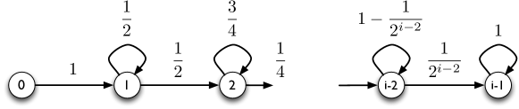
Figure 2: The Markov chain $\mathcal{M}_{i}$ that is used to prove Theorem 8 and Lemma 9: possible depths for item of rank $i$ in the complete tree.

To understand and upper bound $D(i)$, we will use a Markov chain $\mathcal{M}_{i}$ over the integers $0,1,2\dots,i-1$, which denote the possible depths in the Random-Push tree, see Figure 2. For each depth in the chain $0\leq j<i-1$, the probability to move to depth $j+1$ is $2^{-j}$, and the probability to stay at $j$, is $1-2^{-j}$, for $j=i-1$; it is an absorbing state. This chain captures the idea that the probability of an item at level $j$ to be pushed down the tree by a random walk (to level larger than $j$) is $2^{-j}$. The chain does not describe exactly our Random-Push algorithm and $D(i)$, but we will use it to prove an upper bound on $D(i)$. First, we consider a random walk described exactly by the Markov chain $\mathcal{M}_{i}$ with an initial state $0$. Let $\ell(i,w)$ denote the random variable of the last state of a random walk of length $w$ on $\mathcal{M}_{i}$. Then we can show:

Lemma 9

The expected state of $\ell(i,w)$ is such that  $\mathbb{E}[\ell(i,w)]<\lceil\log w\rceil+1$, and $\mathbb{E}[\ell(i,w)]$ is concave in $w$.

To prove Lemma 9 we use the following corollary.

Corollary 10

$$\sum_{i=0}^{w}{w\choose i}(\frac{w-1}{w})^{w-i}\cdot(\frac{1}{w})^{i}\cdot i=1$$

Proof:

$$\sum_{i=0}^{w} {w\choose i}(\frac{w-1}{w})^{w-i}(\frac{1}{w})^{i}i=\sum_{i=1}^{w}{w\choose i}(\frac{w-1}{w})^{w-i}(\frac{1}{w})^{i}i$$

$$=\sum_{i=1}^{w}\frac{w!}{i!\ (w-i)!}(\frac{w-1}{w})^{w-i}(\frac{1}{w})^{i}i=\sum_{i=1}^{w}\frac{(w-1)!}{(i-1)!\ (w-i)!}(\frac{w-1}{w})^{w-i}(\frac{1}{w})^{i-1}$$

$$=\sum_{\eta=0}^{w-1}\frac{(w-1)!}{\eta!\ (w-1-\eta)!}(\frac{w-1}{w})^{w-1-\eta}(\frac{1}{w})^{\eta}~{}~{}~{}\text{(put $i=\eta+1$)}$$

$$=\left(\frac{1}{w}+\frac{w-1}{w}\right)^{w-1}=1$$

$\Box$

Proof:[Proof of Lemma 9] First note that $\mathbb{E}[\ell(i,w)]$ is strictly monotonic in $w$ and can be shown to be concave using the decreasing rate of increase: for $w_{1}<w_{2}$, $\mathbb{E}[\ell(i,w_{1})]-\mathbb{E}[\ell(i,w_{1}-\Delta)]\geq\mathbb{E}[\ell(i,w_{2})]-\mathbb{E}[\ell(i,w_{2}-\Delta)]$. To bound $\mathbb{E}[\ell(i,w)]$, we consider the state of another random walk, $\ell^{\prime}(i,w)$, that starts on state $k=\lceil\log w\rceil$ in a modified chain $\mathcal{M}^{\prime}_{i}$. The modified chain $\mathcal{M}^{\prime}_{i}$ is identical to $\mathcal{M}_{i}$ up to state $k$, but for all states $j>k$, the probability to move to state $j+1$ is $\frac{1}{w}>2^{-k}$ and the probability to stay at $j$ is $\frac{w-1}{w}<1-2^{-k}$. So clearly the walk on $\mathcal{M}^{\prime}_{i}$ makes faster progress than the walk on $\mathcal{M}_{i}$ from state $k$ onward. The expected progress of the walk on $\mathcal{M}^{\prime}_{i}$ which starts from state $k$, is now easier to bound and can shown to be: $\mathbb{E}[\ell^{\prime}(i,w)]\leq\sum_{j=0}^{w}j{w\choose j}(\frac{w-1}{w})^{w-j}(\frac{1}{w})^{j}=1$. But since $\ell(i,w)$ starts at state $0$, we have $\mathbb{E}[\ell(i,w)]<\mathbb{E}[\ell^{\prime}(i,w)]\leq k+1=\lceil\log w\rceil+1$. $\Box$

Next, in Lemma 12, we bound the expected number of times that $v$ could potentially be pushed down by a random push, i.e., the number of requests to elements at a lower depth than $v$. Later we will use this as the length $w$ of the random walk on $\mathcal{M}_{i}$. But, to do so we first state the following lemma.

Lemma 11

For every $\sigma,t$ and $i>j$, we have that in Random-Push, $\mathbb{E}[D(i)]>\mathbb{E}[D(j)]$.

Proof: Let $u$ be an item with rank $j<i$. Hence, it was requested more recently than $v$ (which has rank $i$). The inequality follows from the fact that conditioning that $v$ and $u$ first reached the same depth (after the last request of $u$) then by symmetry their expected progress of depth will be the same from that point. More formally, let $D_{uv}$ be a random variable that denotes the depth when $u$’s depth equals the depth of $v$ for the first time (since the last request of $u$ where its depth is set to 0); and $-1$ if this never happens. Then by the law of total probability,

$$\mathbb{E}[D(i)]=\mathbb{E}_{D_{uv}}[\mathbb{E}[D(i)\mid D_{uv}]]=\sum_{k=-1}^{i-1}\mathbb{P}(D_{uv}=k)\sum_{\ell=0}^{i-1}\ell\cdot\mathbb{P}(D(i)=\ell\mid D_{uv}=k)$$

(and similar for $D(j)$). But since the random walk (i.e., push) is independent of the servers’ ranks, we have for $k\geq 0$ that $\mathbb{E}[D(i)\mid D_{uv}=k]\geq\mathbb{E}[D(j)\mid D_{uv}=k]$. But additionally there is the possibility that they will never be at the same depth (after the last request of $u$) and that $v$ will always have a higher depth, so $\mathbb{E}[D(i)\mid D_{uv}=-1]>\mathbb{E}[D(j)\mid D_{uv}=-1]$. The claim follows. $\Box$

Now, let $W_{i}$ be a random variable that denotes the number of requests for items with higher depth than $v$, since $v$’s last request until time $t$. The following lemma bounds the number of such requests.

Lemma 12

The expected number of requests for items with higher depth than $v$, since $v$ was last requested, is bounded by $\mathbb{E}[W_{i}]\leq 2i-1$.

Proof: We can divide $W_{i}$ into two types of requests: $W_{i}^{>}$ requests for items with higher rank and depth than $v$ at the time of their request, and $W_{i}^{<}$ requests for items with lower rank but higher depth than $v$ at the time of their request. Then $W_{i}=W_{i}^{>}+W_{i}^{<}$. Clearly $W_{i}^{>}\leq i$ since every such request increases the rank of $v$ and this happens $i$ times (note that some of these requests may have lower depth than $v$). $W_{i}^{<}$ is harder to analyze. How many requests for items are there that have lower rank than $v$ at the time of the request, but are below $v$ in the tree (i.e., have higher depth than $v$)? Note that such requests do not increase $v$’s rank, but may increase its depth. Let $u$ be an item with rank $j<i$, hence $u$ was more recently requested than $v$ (maybe several times). Let $X_{j}$ denote the number of requests for $u$ (since $v$ was last requested) in which it had a higher depth than $v$. Then $W_{i}^{<}=\sum_{j=1}^{i-1}X_{j}$. We now claim that $\mathbb{E}[X_{j}]\leq 1$. Assume by contradiction that $\mathbb{E}[X_{j}]>1$. But then this implies that we can construct a sequence $\sigma^{\prime}$ for which the expected depth of $u$ will be larger than the expected depth of $v$, contradicting Lemma 11. Putting it all together:

$$\mathbb{E}[W_{i}]=\mathbb{E}[W_{i}^{>}+W_{i}^{<}]\leq\mathbb{E}[i]+\mathbb{E}[\sum_{n=1}^{i-1}X_{n}]\leq i+\sum_{n=1}^{i-1}\mathbb{E}[X_{n}]\leq 2i-1$$

$\Box$

We now have all we need to prove Theorem 8. The proof follows by showing that $\mathbb{E}[D(i)]\leq\log i+3$.

Proof:[Proof of Theorem 8] Let $D(i,w)$ be a random variable that denotes the depth of $v$ conditioning that there are $w$ requests of items with higher depth than $v$, since the last request for $v$. Note that by the total probability law, we have that

$$\mathbb{E}[D(i)]=\mathbb{E}_{W_{i}}[\mathbb{E}[D(i,W_{i})]=\sum_{w=1}^{\lvert\sigma\rvert}\mathbb{P}(W_{i}=w)\mathbb{E}[D(i,W_{i}=w)]$$

Next we claim that $D(i,w)$ is stochastically less [28] than $\ell(i,w)$, denoted by $D(i,w)\preceq\ell(i,w)$.

This is true since the transition probabilities (to increase the depth) in the Markov chain $\mathcal{M}_{i}$ are at least as high as in the Markov chain that describes $D(i,w)$. The probability that a random walk to depth higher than $v$’s depth visits $v$ (and pushes it down) is exactly $2^{-j}$ where $j$ is the depth of $v$. Since $D(i,w)\preceq\ell(i,w)$, it will then follow from Theorem 14 that $\mathbb{E}[D(i,w)]\leq\mathbb{E}[\ell(i,w)]$. Clearly we also have $\mathbb{E}_{W_{i}}\mathbb{E}[D(i,W_{i})]\leq\mathbb{E}_{W_{i}}\mathbb{E}[\ell(i,W_{i})]$. Let $f_{i}(W_{i})=\mathbb{E}[\ell(i,W_{i})]$ be a random variable which is a function of the random variable $W_{i}$. Recall that $f_{i}()$ is concave, then by Jensen’s inequality [15] and Lemma 12 we get:

$$\mathbb{E}[D(i)] =\mathbb{E}_{W_{i}}[\mathbb{E}[D(i,W_{i})]]\leq\mathbb{E}_{W_{i}}[\mathbb{E}[\ell(i,W_{i})]]=\mathbb{E}_{W_{i}}[f_{i}(W_{i})]\leq f_{i}(\mathbb{E}[W_{i}])$$

$$\leq f_{i}(2i-1)=\mathbb{E}[\ell(i,2i-1)]\leq\lceil\log 2i\rceil+1\leq\log i+3$$

$\Box$

1:   access $s=u.\mathrm{host}$ along tree branches             (cost: $u.\mathrm{dep}$)

2:   let $v=s_{1}.\mathrm{guest}$ be the item at the current root

3:   move $u$ to the root server $s_{1}$, setting $s_{1}.\mathrm{guest}=u$ (cost: $u.\mathrm{dep}$)

4:   employ Random-Push to shift down $v$ to depth $s.\mathrm{dep}$ (cost: $u.\mathrm{dep}$)

5:   let $w$ be the item at the end of the push-down path, where $w.\mathrm{dep}=s.\mathrm{dep}$

6:   move $w$ to $s$, i.e., setting $s.\mathrm{guest}=w$            (cost: $u.\mathrm{dep}\times 2$)

Algorithm 2 Upon access to $u$ in Push-Down Tree

It now follows almost directly from Theorems 7 and 8 that Random-Push is dynamically optimal.

See 3 Proof: Let the $t$-th requested item have rank $r_{t}$, then the access cost is $D(r_{t})$. According to the Random-Push (Algorithm 2), the total cost is $5D(r_{t})$ which is five times the access cost on the MRU$(4)$ tree. Formally, using Theorem  7 and Theorem 8, the expected total cost is:

$$\mathbb{E}\left[\mathrm{cost}(\textsc{Random-Push})\right] =\mathbb{E}\left[\sum_{i=1}^{t}5D(r_{i})\right]=5\sum_{i=1}^{t}\mathbb{E}\left[D(r_{i})\right]\leq 5\sum_{i=1}^{t}(\log(r_{i})+3)$$

$$\leq 5\sum_{i=1}^{t}(\lfloor\log(r_{i})\rfloor+4)\leq 5\sum_{i=1}^{t}\mathrm{cost}^{(t)}(\textsc{MRU}(4))$$

$$\leq 5\cdot\mathrm{cost}(\textsc{MRU}(4))=60\cdot\mathrm{cost}(\textsc{Opt})$$

$\Box$

6 Related Work

The self-adjusting tree networks considered in this paper feature an interesting connection to self-adjusting datastructures. A key difference is that while datastructures need to be searchable, networks come with routing protocols: the presence of a map allows us to trivially access a node (or item) at distance $k$ from the front at a cost $k$. Interestingly, while we have shown in this paper that dynamically optimal algorithms for tree networks exist, the quest for constant competitive online algorithms for binary search trees remains a major open problem [31]. Nevertheless, there are self-adjusting binary search trees that are known to be access optimal [9], but their rearrangement cost it too high.

In the following, we first review related work on datastructures and then discuss literature in the context of networks.

Dynamic List Update: Linked List (LL). The dynamically optimal linked list datastructure is a seminal [30] result in the area: algorithms such as Move-To-Front (MTF), which moves each accessed element to the front of the list, are known to be 2-competitive, which is optimal [1, 4, 30]. We note that the Move-To-Front algorithm results in the Most Recently Used property where items that were more recently used are closer to the head of the list. The best known competitive ratio for randomized algorithms for LLs is 1.6, which almost matches the randomized lower bound of 1.5 [3, 32].

Binary Search Tree (BST). In contrast to $\mathrm{CT}$s, self-adjustments in BSTs are based on rotations (which are assumed to have unit cost). While BSTs have the working set property, we are missing a matching lower bound: the Dynamic Optimality Conjecture, the question whether splay trees [31] are dynamically optimal, continues to puzzle researchers even in the randomized case [2]. On the positive side, over the last years, many deep insights into the properties of self-adjusting BSTs have been obtained [14], including improved (but non-constant) competitive ratios [11], regarding weaker properties such as working sets, static, dynamic, lazy, and weighted, fingers, regarding pattern-avoidance [13], and so on. It is also known (under the name dynamic search-optimality) that if the online algorithm is allowed to make rotations for free after each request, dynamic optimality can be achieved [9]. Known lower bounds are by Wilber [33], by Demaine et al. [17]’s interleaves bound (a variation), and by Derryberry et al. [18] (based on graphical interpretations). It is not known today whether any of these lower bounds is tight.

Unordered Tree (UT). We are not the first to consider unordered trees and it is known that existing lower bounds for (offline) algorithms on BSTs also apply to UTs that use rotations: Wilber’s theorem can be generalized [21]. However, it is also known that this correspondance between ordered and unordered trees no longer holds under weaker measures such as key independent processing costs and in particular Iacono’s measure [23]: the expected cost of the sequence which results from a random assignment of keys from the search tree to the items specified in an access request sequence. Iacono’s work is also one example of prior work which shows that for specific scenarios, working set and dynamic optimality properties are equivalent. Regarding the current work, we note that the reconfiguration operations in UTs are more powerful than the swapping operations considered in our paper: a rotation allows to move entire subtrees at unit costs, while the corresponding cost in $\mathrm{CT}$s is linear in the subtree size. We also note that in our model, we cannot move freely between levels, but moves can only occur between parent and child. In contrast to UTs, $\mathrm{CT}$s are bound to be balanced.

Skip List (SL) and B-Trees (BT). Intriguingly, although SLs and BSTs can be transformed to each other [16], Bose et al. [12] were able to prove dynamic optimality for (a restricted kind of) SLs as well as BTs. Similarly to our paper, the authors rely on a connection between dynamic optimality and working set: they show that the working set property is sufficient for their restricted SLs (for BSTs, it is known that the working set is an upper bound, but it is not known yet whether it is also a lower bound). However, the quest for proving dynamic optimality for general skip lists remains an open problem: two restricted types of models were considered in [12], bounded and weakly bounded. In the bounded model, the adversary can never forward more than $B$ times on a given skip list level, without going down in the search; and in the weakly bounded model, the first $i$ highest levels contain no more than $\sum_{j=0}^{i}B^{j}$ elements. Optimality only holds for constant $B$. The weakly bounded model is related to a complete $B$-ary tree (similar to our complete binary tree), but there is no obvious or direct connection between our result and the weakly bounded optimality. Due to the relationship between SLs and BSTs, a dynamically optimal SL would imply a working set lower bound for BST. Moreover, while both in their model and ours, proving the working set property is key, the problems turn out to be fundamentally different. In contrast to SLs, $\mathrm{CT}$s revolve around unordered (and balanced) trees (that do not provide a simple search mechanism), rely on a different reconfiguration operation (i.e., swapping or pushing an item to its parent comes at unit cost), and, as we show in this paper, actually provide dynamic optimality for their general form. Finally, we note that [12] (somewhat implicitly) also showed that a random walk approach can achieve the working set property; in our paper, we show that the working set property can even be achieved deterministically and without maintaining MRU.

Heaps and Paging. More generally, our work is also reminiscent of online paging models for hierarchies of caches [34], which aim to keep high-capacity nodes resp. frequently accessed items close to each other, however, without accounting for the reconfiguration cost over time. Similar to the discussion above, self-adjusting $\mathrm{CT}$s differ from paging models in that in our model, items cannot move arbitrarily and freely between levels (but only between parent and child at unit cost).

Self-Adjusting Networks. Finally, little is known about self-adjusting networks. While there exist several algorithms for the design of static demand-aware networks, e.g. [6, 7, 19, 29], online algorithms which also minimize reconfiguration costs are less explored. The most closely related work to ours are SplayNets [26, 27], which are also based on a tree topology (but a searchable one). However, SplayNets do not provide any formal guarantees over time, besides convergence properties in case of certain fixed demands.

7 Conclusion

This paper presented a deterministic and a randomized online algorithm for a fundamental building block of self-adjusting networked systems based on reconfigurable topologies. We believe that our paper opens several interesting avenues for future research, e.g., related to the design of fully decentralized and self-adjusting communication networks based on more general topologies and serving more general communication patterns.

Acknowledgments. Research supported by the ERC Consolidator grant AdjustNet (agreement no. 864228).

Appendix

8 Optimal Fixed Trees

The key difference between binary search trees and binary trees is that the latter provides more flexibilities in how items can be arranged on the tree. Accordingly, one may wonder whether more flexibilities will render the optimal data structure design problem algorithmically simpler or harder.

In this section, we consider the static problem variant, and investigate offline algorithms to compute optimal trees for a fixed frequency distribution over the items. To this end, we assume that for each item $v$, we are given a frequency $v.\mathrm{freq}$, where $\sum_{v\in V}v.\mathrm{freq}=1$.

Definition 7 (Optimal Fixed Tree)

We call a tree optimal static tree if it minimizes the expected path length $\sum_{i\in[1,n]}(v_{i}.\mathrm{freq}\cdot v_{i}.\mathrm{dep})$.

Our objective is to design an optimal static tree according to Definition 7. Now, let us define the following notion of Most Frequently Used (MFU) tree which keeps items of larger empirical frequencies closer to the root:

Definition 8 (MFU Tree)

A tree in which for every pair of items $v_{i},v_{j}\in V$, it holds that if $v_{i}.\mathrm{freq}\geq v_{j}.\mathrm{freq}$ then $v_{i}.\mathrm{dep}\leq v_{j}.\mathrm{dep}$, is called MFU tree.

Observe that MFU trees are not unique but rather, there are many MFU trees. In particular, the positions of items at the same depth can be changed arbitrarily without violating the MFU properties.

Theorem 13 (Optimal Fixed Trees)

Any MFU tree is an optimal fixed tree.

Proof: Recall that by definition, MFU trees have the property that for all node pairs $v_{i},v_{j}$: $v_{i}.\mathrm{freq}>v_{j}.\mathrm{freq}\Rightarrow v_{i}.\mathrm{dep}\leq v_{j}.\mathrm{dep}$. For the sake of contradiction, assume that there is a tree $T$ which achieves the minimum expected path length but for which there exists at least one item pair $v_{i},v_{j}$ which violates our assumption, i.e., it holds that $v_{i}.\mathrm{freq}>v_{j}.\mathrm{freq}$ but $v_{i}.\mathrm{dep}>v_{j}.\mathrm{dep}$. From this, we can derive a contradiction to the minimum expected path length: by swapping the positions of items $v_{i}$ and $v_{j}$, we obtain a tree $T^{\prime}$ with an expected path length which is shorter by $\mathrm{cost}(T,\sigma)-\mathrm{cost}(T^{\prime},\sigma)=$ $v_{i}.\mathrm{freq}\cdot v_{i}.\mathrm{dep}+v_{j}.\mathrm{freq}\cdot v_{j}.\mathrm{dep}-v_{i}.\mathrm{freq}\cdot v_{j}.\mathrm{dep}+v_{j}.\mathrm{freq}\cdot v_{i}.\mathrm{dep}$ $>0$. $\Box$

MFU trees can also be constructed very efficiently, e.g., by performing the following ordered insertion: we insert the items into the tree $T$ in a top-down, left-to-right manner, in descending order of their frequencies (i.e., item $v_{i}$ is inserted before item $v_{j}$ if $v_{i}.\mathrm{freq}>v_{j}.\mathrm{freq}$).

9 Stochastic Domination

We recall some of the known results related to Stochastic Domination [28].

Definition 9 (Stochastic Domination)

Let ${\tt X}$ and ${\tt Y}$ be two random variables, not necessarily on the same probability space. The random variable ${\tt X}$ is stochastically smaller than ${\tt Y}$, denoted by ${\tt X}\preceq{\tt Y}$, if $\mathbb{P}[{\tt X}>z]\leq\mathbb{P}[{\tt Y}>z]$ for every $z\in\mathbb{R}$. If additionally $\mathbb{P}[{\tt X}>z]<\mathbb{P}[{\tt Y}>z]$ for some $z$, then ${\tt X}$ is stochastically strictly less than ${\tt Y}$, denoted by ${\tt X}\prec{\tt Y}$.

Theorem 14 (Stochastic Order)

Let ${\tt X}$ and ${\tt Y}$ be two random variables, not necessarily on the same probability space.

1. Suppose ${\tt X}\prec{\tt Y}$. Then $\mathbb{E}[U({\tt X})]<\mathbb{E}[U({\tt Y})]$ for any strictly increasing function $U$.

2. Suppose ${\tt X}_{1}\prec{\tt Y}_{1}$ and ${\tt X}_{2}\prec{\tt Y}_{2}$, for four random variables ${\tt X}_{1},{\tt Y}_{1},{\tt X}_{2}$ and ${\tt Y}_{2}$. Then $a{\tt X}_{1}+b{\tt Y}_{1}\prec a{\tt X}_{2}+b{\tt Y}_{2}$ for any two constants $a,b>0$.

3. Suppose $U$ is a non-decreasing function and ${\tt X}\prec{\tt Y}$ then $U({\tt X})\prec U({\tt Y})$.

4. Given that ${\tt X}$ and ${\tt Y}$ follow the binomial distribution, i.e., ${\tt X}\sim Bn(n_{1},p_{1})$ and ${\tt Y}\sim Bn(n_{2},p_{2})$, then ${\tt X}\preceq{\tt Y}$ if and only if the following two conditions holds: $(1-p_{1})^{n_{1}}\geq(1-p_{2})^{n_{2}}$ and $n_{1}\leq n_{2}$.

References

- [1] Susanne Albers. A competitive analysis of the list update problem with lookahead. Mathematical Foundations of Computer Science 1994, pages 199–210, 1994.
- [2] Susanne Albers and Marek Karpinski. Randomized splay trees: theoretical and experimental results. Information Processing Letters, 81(4):213–221, 2002.
- [3] Susanne Albers, Bernhard Von Stengel, and Ralph Werchner. A combined bit and timestamp algorithm for the list update problem. Information Processing Letters, 56(3):135–139, 1995.
- [4] Susanne Albers and Jeffery Westbrook. Self-organizing data structures. In Online algorithms, pages 13–51. Springer, 1998.
- [5] Chen Avin, Manya Ghobadi, Chen Griner, and Stefan Schmid. On the complexity of traffic traces and implications. In Proc. ACM SIGMETRICS, 2020.
- [6] Chen Avin, Kaushik Mondal, and Stefan Schmid. Demand-aware network designs of bounded degree. Distributed Computing, 2017.
- [7] Chen Avin, Kaushik Mondal, and Stefan Schmid. Demand-aware network design with minimal congestion and route lengths. In Proc. IEEE INFOCOM, pages 1351–1359, 2019.
- [8] Chen Avin and Stefan Schmid. Toward demand-aware networking: A theory for self-adjusting networks. ACM SIGCOMM Computer Communication Review, 48(5):31–40, 2019.
- [9] Avrim Blum, Shuchi Chawla, and Adam Kalai. Static optimality and dynamic search-optimality in lists and trees. In Proc. 13th Annual ACM-SIAM Symposium on Discrete Algorithms (SODA), 2002.
- [10] Shaileshh Bojja Venkatakrishnan, Mohammad Alizadeh, and Pramod Viswanath. Costly circuits, submodular schedules and approximate carathéodory theorems. In Proceedings of the 2016 ACM SIGMETRICS International Conference on Measurement and Modeling of Computer Science, pages 75–88, 2016.
- [11] Prosenjit Bose, Karim Douïeb, Vida Dujmović, and Rolf Fagerberg. An o (log log n)-competitive binary search tree with optimal worst-case access times. In Scandinavian Workshop on Algorithm Theory, pages 38–49. Springer, 2010.
- [12] Prosenjit Bose, Karim Douïeb, and Stefan Langerman. Dynamic optimality for skip lists and b-trees. In Proc. 19th Annual ACM-SIAM Symposium on Discrete Algorithms (SODA), pages 1106–1114, 2008.
- [13] Parinya Chalermsook, Mayank Goswami, László Kozma, Kurt Mehlhorn, and Thatchaphol Saranurak. Pattern-avoiding access in binary search trees. In Proc. Foundations of Computer Science (FOCS), 2015 IEEE 56th Annual Symposium on, pages 410–423. IEEE, 2015.
- [14] Parinya Chalermsook, Mayank Goswami, László Kozma, Kurt Mehlhorn, and Thatchaphol Saranurak. The landscape of bounds for binary search trees. arXiv preprint arXiv:1603.04892, 2016.
- [15] T.M. Cover and J. Thomas. Elements of information theory. Wiley, 2006.
- [16] Brian C. Dean and Zachary H. Jones. Exploring the duality between skip lists and binary search trees. In Proceedings of the 45th Annual Southeast Regional Conference, ACM-SE 45, pages 395–399, New York, NY, USA, 2007. ACM.
- [17] Erik D. Demaine, Dion Harmon, John Iacono, and Mihai Patrascu. Dynamic optimality - almost. SIAM J. Comput., 37(1):240–251, 2007.
- [18] Jonathan Derryberry, Daniel Dominic Sleator, and Chengwen Chris Wang. A lower bound framework for binary search trees with rotations. School of Computer Science, Carnegie Mellon University, 2005.
- [19] Klaus-Tycho Foerster, Monia Ghobadi, and Stefan Schmid. Characterizing the algorithmic complexity of reconfigurable data center architectures. In Proc. ACM/IEEE Symposium on Architectures for Networking and Communications Systems (ANCS), 2018.
- [20] Klaus-Tycho Foerster and Stefan Schmid. Survey of reconfigurable data center networks: Enablers, algorithms, complexity. In SIGACT News, 2019.
- [21] Michael L Fredman. Generalizing a theorem of wilber on rotations in binary search trees to encompass unordered binary trees. Algorithmica, 62(3-4):863–878, 2012.
- [22] Navid Hamedazimi, Zafar Qazi, Himanshu Gupta, Vyas Sekar, Samir R Das, Jon P Longtin, Himanshu Shah, and Ashish Tanwer. Firefly: A reconfigurable wireless data center fabric using free-space optics. In Proc. ACM SIGCOMM Computer Communication Review (CCR), volume 44, pages 319–330, 2014.
- [23] John Iacono. Key-independent optimality. Algorithmica, 42(1):3–10, 2005.
- [24] Srikanth Kandula, Sudipta Sengupta, Albert Greenberg, Parveen Patel, and Ronnie Chaiken. The nature of data center traffic: measurements & analysis. In Proc. 9th ACM Internet Measurement Conference (IMC), pages 202–208, 2009.
- [25] M. Ghobadi et al. Projector: Agile reconfigurable data center interconnect. In Proc. ACM SIGCOMM, pages 216–229, 2016.
- [26] Bruna Peres, A de O Otavio, Olga Goussevskaia, Chen Avin, and Stefan Schmid. Distributed self-adjusting tree networks. In Proc. IEEE INFOCOM, pages 145–153, 2019.
- [27] Stefan Schmid, Chen Avin, Christian Scheideler, Michael Borokhovich, Bernhard Haeupler, and Zvi Lotker. Splaynet: Towards locally self-adjusting networks. IEEE/ACM Trans. Netw., 24(3):1421–1433, June 2016.
- [28] Moshe Shaked and J George Shanthikumar. Stochastic orders. Springer Science & Business Media, 2007.
- [29] Ankit Singla, Atul Singh, Kishore Ramachandran, Lei Xu, and Yueping Zhang. Proteus: a topology malleable data center network. In Proc. ACM Workshop on Hot Topics in Networks (HotNets), 2010.
- [30] Daniel D. Sleator and Robert E. Tarjan. Amortized efficiency of list update and paging rules. Commun. ACM, 28(2):202–208, February 1985.
- [31] Daniel Dominic Sleator and Robert Endre Tarjan. Self-adjusting binary search trees. J. ACM, 32(3):652–686, July 1985.
- [32] Boris Teia. A lower bound for randomized list update algorithms. Information Processing Letters, 47(1):5–9, 1993.
- [33] Robert Wilber. Lower bounds for accessing binary search trees with rotations. SIAM Journal on Computing, 18(1):56–67, 1989.
- [34] Gala Yadgar, Michael Factor, Kai Li, and Assaf Schuster. Management of multilevel, multiclient cache hierarchies with application hints. ACM Transactions on Computer Systems (TOCS), 29(2):5, 2011.