Entanglement hamiltonian evolution during thermalization in conformal field theory

Abstract

In this work, we study the time evolution of the entanglement hamiltonian during the process of thermalization in a (1+1)-dimensional conformal field theory (CFT) after a quantum quench from a special class of initial states. In particular, we focus on a subsystem which is a finite interval at the end of a semi-infinite line. Based on conformal mappings, the exact forms of both entanglement hamiltonian and entanglement spectrum of the subsystem can be obtained. Aside from various interesting features, it is found that in the infinite time limit the entanglement hamiltonian and entanglement spectrum are exactly the same as those in the thermal ensemble. The entanglement spectrum approaches the steady state spectrum exponentially in time. We also study the modular flows generated by the entanglement hamiltonian in Minkowski spacetime, which provides us with an intuitive picture of how the entanglement propagates and how the subsystem is thermalized. Furthermore, the effect of a generic initial state is also discussed.

Contents

toc

1 Introduction

1.1 Introduction

Quantum quench and thermalization

Unraveling non-equilibrium dynamics in quantum many-body systems remains an important open question. A paradigmatic protocol for non-equilibrium dynamics, which will be our focus here, is a quantum quench, in which one changes a system’s hamiltonian as a function of time. In typical settings, the time-dependent hamiltonian $H(t)$ interpolates between two hamiltonians, $H(t\to-\infty)\equiv H_{i}$ and $H(t\to\infty)\equiv H_{f}$, and the change in the hamiltonian occurs during a given finite time scale. In the simplest case, one considers a sudden quantum quench, where $H(t)=H_{i}$ for $t<0$ and $H(t)=H_{f}$ for $t>0$. One then follows the time evolution of a quantum state $|\psi(t)\rangle$, which is initially in the ground state of $H_{i}$, and is then later evolved by $H_{f}$.

While predicting and classifying the behaviors of $|\psi(t)\rangle$ are daunting tasks in general, if the dynamics described by the hamiltonian $H_{f}$ is sufficiently ergodic (chaotic), it is expected that the late time behaviors of the state $|\psi(t)\rangle$ are well captured by the thermal state – the state $|\psi(t)\rangle$ thermalizes at late times [1, 2, 3, 4, 5, 6, 7]. For systems which are not chaotic, e.g., integrable systems, it is expected that the late time behavior of the system after a quantum quench is characterized by the generalized Gibbs ensemble (GGE) [8], which has been studied in some solvable models [9].

Quantum quench and thermalization in (1+1)d CFT

Quantum quenches and thermalization in the context of (1+1)-dimensional conformal field theory (CFTs) have been studied in the literature. In Ref. [33], thermalization after a global quantum quench is studied based on the two- and higher point correlation function of local operators. It is found that when all these local operators fall into the light cone, the correlation function becomes stationary and equals its value in the thermal ensemble up to exponentially small corrections. Later in Ref. [34], Cardy calculated the overlap between the reduced density matrix after thermalization (introduced by a global quench) and that in the thermal ensemble, and found the overlap is exponentially close to unity. In the same work, the effect of a deformation of the initial state and of the CFT hamiltonian was also studied. See also Ref. [35] for a related discussion.

Setup, purpose and main results of this paper

In this paper, we will have a further look at thermalization in (1+1)d CFTs, by focusing on the time evolution of the entanglement hamiltonian and its spectrum for a given finite subregion $A$ of the total system.

To be specific, we will focus on the following setup for a global quantum quench summarized in Fig.1. Our system is semi-infinite with a physical boundary at $x=0$. At time $t=0$, we start from an initial state with short-range correlations (short-range entangled), which may be considered the ground state of a gapped hamiltonian. We then quench into a CFT; the state after $t=0$ will then be time-evolved with the hamiltonian $H_{{\rm CFT}}$ which is the hamiltonian of a CFT in semi-infinite space with a boundary at $x=0$. Of interest to us is quantum entanglement between two subregions $A$ and $B$. We choose subregion $A$ to be a finite interval of length $L$ at the end of the total system, i.e. $A=[0,L]$, whereas the complement $B=(L,\infty)$ of $A$ is semi-infinite. It is expected that the finiteness of subsystem $A$ and the semi-infinite size of the complement $B$ (the ”bath”) may result in thermalization after a quantum quench, as discussed shortly.

In order to diagnose thermalization in this setup, we will study (i) the entanglement hamiltonian for the finite subregion $A$, (ii) its entanglement spectrum, and, in addition, (iii) the fictitious real time-evolution generated by the entanglement hamiltonian, which can be visualized by a (Killing) vector field in Minkowski spacetime. For simplicity, we refer to the latter as the “modular flow” (as it is conventionally done). As we will demonstrate, following the time-dependence of these quantities provides detailed information about the thermalization process.

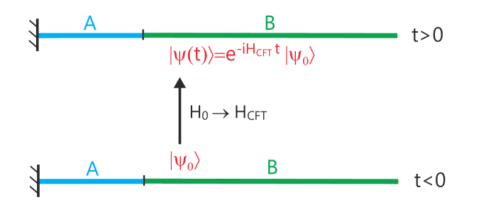
Figure 1: Setup of the global quantum quench in this work. The total system is defined along $[0,\infty)$ and the subsystem $A$ lives on the finite interval $[0,L]$, at the end of the total semi-infinite system. One starts from a short-range entangled state $|\psi_{0}\rangle$, which may be viewed as the ground state of a gapped hamiltonian $H_{0}$. At $t=0$, we switch the hamiltonian to $H_{\text{CFT}}$, and the state $|\psi(t>0)\rangle$ evolves as $|\psi(t)\rangle=e^{-iH_{\text{CFT}}t}|\psi_{0}\rangle$.

The main results of this work are summarized as follows:

(i) By choosing the short-range entangled initial state as a regularized conformally invariant boundary state, corresponding to a conformal boundary condition that is the same as that characterizing the physical boundary at the left end of the semi-infinite spatial region at position $x=0$ (see Fig. 1), we find that in the limit $t\to\infty$ the entanglement hamiltonian and its spectrum for subsystem $A=[0,L]$ are exactly the same as those in a thermal ensemble for $H_{CFT}$ with finite temperature $\beta^{-1}$. The entanglement spectrum approaches this steady state spectrum exponentially in time for $t>L$.

(ii) We also study the modular flows generated by the entanglement hamiltonian in Minkowski spacetime. These flows show different features in the regime where $t<L$ as compared to the regime $t>L$. For $t<L$, these flows evolve in time and tell us how the entanglement propagates; for $t>L$, these flows become stationary and exhibit the features of the thermal ensemble, indicating thermalization of the subsystem.

(iii) We also study the effect of a generic initial state. When the conformally invariant boundary state describing the short-range entangled initial state is different from that describing the physical boundary condition at the end $x=0$ of the semi-infinite space, the entanglement spectrum of subsystem $A=[0,L]$ is not exactly the same, in the long time limit $t\to\infty$, as that in the thermal ensemble. There is an order $\mathcal{O}(1)$ difference in the entanglement entropy $S_{A}$ as compared to the situation discussion in (i) above.

1.2 Entanglement and entanglement hamiltonian

For the rest of this section, we will introduce necessary concepts and terminologies which will be used throughout the paper.

We first recall the definitions of the entanglement hamiltonian or modular hamiltonian, which play an important role in understanding quantum entanglement in many-body systems and quantum field theories. For example, the spectrum of the entanglement hamiltonian, also called entanglement spectrum, is useful for characterizing and classifying gapped quantum many-body states [10, 11, 12, 13, 14]. The entanglement hamiltonian is also important for studying the relative entropy and first law of entanglement [15].

Given the reduced density matrix $\rho_{A}$ defined for a given subregion $A$, which encodes all the information on the observables localized in the subregion $A$, the entanglement hamiltonian $K_{A}$ is defined by

$$\rho_{A}=e^{-2\pi K_{A}},\quad\text{or}\quad K_{A}=-\frac{1}{2\pi}\log\rho_{A}.$$ (1)

Apparently, the knowledge of the entanglement hamiltonian $K_{A}$ is equivalent to that of the reduced density matrix $\rho_{A}$. In particular, the spectrum of $K_{A}$ determines all the Renyi entropies and the von-Neumann entropy as follows

$$S_{A}^{(n)}=\frac{1}{1-n}\log\text{Tr}_{A}e^{-2\pi nK_{A}},\quad S_{A}=\lim_{n\to 1}S_{A}^{(n)}=2\pi\text{Tr}_{A}\left(K_{A}e^{-2\pi K_{A}}\right).$$ (2)

Although difficult to obtain in general, there are some specific cases in relativistic quantum field theories where $K_{A}$ can be explicitly expressed as an integral of local operators. One basic example is the reduced density matrix for half-space $x_{1}>0$ of the ground state of a relativistic quantum field theory in infinite $d$-dimensional (position) space. Its entanglement hamiltonian can be expressed as $K_{A}=\int_{x_{1}>0}x_{1}T_{00}(x)d^{d-1}x$ [17, 18], where $T_{00}(x)$ denotes the local energy density operator, i.e. the ‘time-time’ component of the energy momentum tensor. Other interesting cases include spherical regions in CFTs [19], regions in a thermal ensemble in CFTs [20], $n$ disjoint intervals for a two dimensional massless Dirac field [21, 22, 23], the Ising chain away from criticality [24], a free-fermion chain with arbitrary filling [25], and a variety of one- and two-dimensional lattice models [26, 27, 28], etc.. To our knowledge, entanglement hamiltonians for time dependent cases were not studied until the most recent work by Cardy and Tonni [29], where both global and local quantum quenches in (1+1)d CFTs were considered. (We will give a brief overview of their approach below.)

1.3 Quasi particle picture

A detailed analysis of the entanglement hamiltonian, the entanglement spectrum, and the modular flow in our setup will be presented in the following sections. Here, we present a simple physical picture for entanglement propagation based on the quasi-particle picture (Fig. 2). While there is no a priori reason for the quasi particle picture to hold for generic interacting CFTs when the central charge is sufficiently large[30], it allows us to find that most of the results in this paper, including the time evolution of entanglement hamiltonians and modular flows in Minkowski spacetime, can be straightforwardly understood in terms of this picture. In particular, we readily identify three different time regimes as follows.

At $t=0$, the entanglement between $A$ and $B$ originates mainly from the region near the entangling point, i.e., from positions $x$ satisfying $|x-L|\sim\beta$. (Here $\beta$ measures the correlation length of the initial state.). After $t=0$, quasiparticles are emitted from each point of the system. The entanglement is carried between the left-moving and right-moving quasiparticles which propagate in opposite directions with the speed of light $c=1$. As shown in Fig.  2, by focusing on the distribution of quasiparticles in subsystem $A$, there are mainly three interesting time regimes:

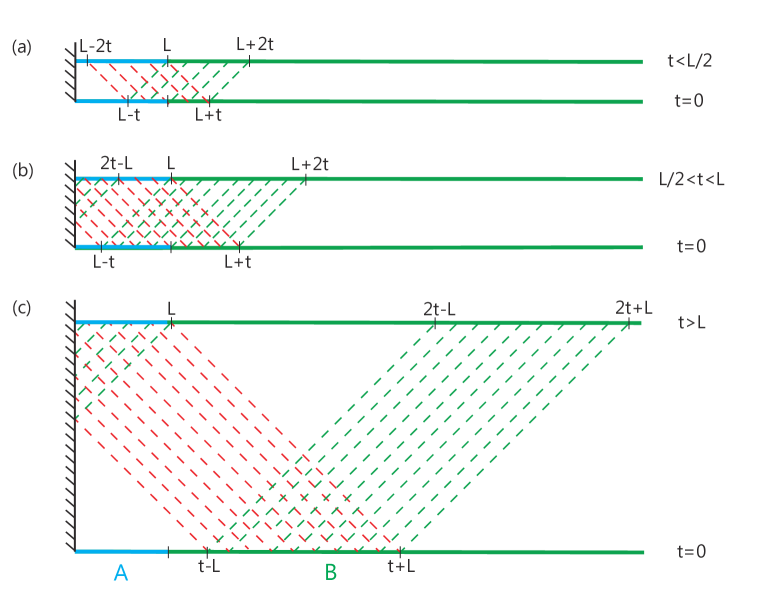
Figure 2: Quasiparticle picture describing the entanglement between $A=[0,L]$ and $B=(L,\infty)$ after a global quantum quench. Here we focus on the quasiparticles in subsystem $A$. (a) For $t<L/2$, only the left-moving quasiparticles (red dotted line) in subinterval $(L-2t,L)$ contribute to the entanglement between $A$ and $B$. These quasiparticles are entangled with the right-moving ones in subinterval $(L,L+2t)$. (b) For $L/2<t<L$, due to reflection from the physical boundary at $x=0$, both the right-moving quasiparticles (green dotted line) in subinterval $[0,2t-L)$ and the left-moving quasiparticles in interval $[0,L]$ contribute to the entanglement. They are entangled with the right-moving quasiparticles in subinterval $(L,L+2t)$. (c) For $t>L$, the entanglement between $A$ and $B$ is saturated. Both the left-moving and right moving quasiparticles in $[0,L]$ contribute to the entanglement. These quasiparticles are entangled with the right-moving ones in subinterval $[2t-L,2t+L]$.

1. For $t<L/2$, only the left-moving quasiparticles distributed in subinterval $[L-2t,L]$ contribute to the entanglement between $A$ and $B$. At these times $t$, these quasiparticles are entangled with those which are right-moving and located in subinterval $[L,L+2t]$ of subsystem $B$.

2. For $L/2<t<L$, both the left-moving quasiparticles in $[0,L]$ and the right-moving quasiparticles in $[0,2t-L]$ contribute to the entanglement . These quasiparticles are entangled with the right-moving ones in region $[L,L+2t]$ of subsystem $B$.

3. For $t>L$, both the left-moving and the right-moving quasiparticles in the whole region of subsystem $A=[0,L]$ contribute to the entanglement, and they are entangled with the right-moving quasiparticles in region $[2t-L,2t+L]$ of subsystem $B$. In particular, the entanglement entropy $S_{A}$ ($S_{B}$) of subsystem $A$ ($B$) is saturated because the number of quasiparticles that contribute to $S_{A}$ ($S_{B}$) does no longer increase.

1.4 Global quantum quench in (1+1)d CFTs

In CFTs, the entanglement hamiltonian and its spectrum can often be obtained by making use of conformal mapping. Let us now first review this approach used by Cardy and Tonni [29], focusing on global quantum quenches in an infinite system.

One starts from an initial state $|\psi_{0}\rangle$ and evolves it with a hamiltonian as $e^{-iHt}|\psi_{0}\rangle$. Here we choose $H=H_{\text{CFT}}$. To simplify this problem, one can choose an initial state of the form $|\psi_{0}\rangle=e^{-(\beta/4)H_{\rm{CFT}}}|b\rangle$ where $|b\rangle$ is a conformal boundary state. The conformal boundary state is a non-normalizable state with no real-space entanglement [36]. Evolving $|b\rangle$ with a small amount of (imaginary) time $\beta/4$, introduces a finite (small) real space entanglement and the state $e^{-(\beta/4)H_{\rm{CFT}}}|b\rangle$ becomes normalizable . Physically, the parameter $\beta$ can be interpreted as the correlation length of the initial state. Throughout this work, we are interested in the limit $L\gg\beta$. The time dependent density matrix has the form $\rho(t)\propto e^{-iHt}e^{-(\beta/4)H_{\rm{CFT}}}|b\rangle\langle b|e^{-(\beta/4)H_{\rm{CFT}}}e^{iHt}.$ We will work in Euclidean spacetime, i.e. with

$$\rho(\tau)\propto e^{-H\tau}e^{-(\beta/4)H_{\rm{CFT}}}|b\rangle\langle b|e^{-(\beta/4)H_{\rm{CFT}}}e^{+H\tau}.$$ (3)

Quantities such as entanglement entropy, correlation functions of operators and so on can be evaluated based on $\rho(\tau)$. To obtain the real time evolution, we simply need to take an analytical continuation $\tau\to it$ in the final step.

In a space-time path integral picture, $\rho(\tau)$ in Eq. (3) can be represented as a path integral in a strip of width $\beta/2$, as shown in Fig. 3, where we choose $A=[0,\infty)$ and $B=(-\infty,0)$. Here, the reduced density matrix $\rho_{A}=\text{Tr}_{B}\,\rho$ is obtained by sewing together the degrees of freedom in $B$, and then there is a branch cut along $C=\{i\tau+x,x\geq 0\}$. To introduce regularization, we remove a small disc at the entangling point $z_{0}=i\tau+0$. Then the strip (with the small disk removed) can be mapped to an annulus in the $w$-plane after a conformal mapping $w=f(z)$. The circumference along the periodic $v=\text{Im}\,w$ direction is $2\pi$, and the width of the annulus along the $u=\text{Re}\,w$ direction is denoted by $W$.

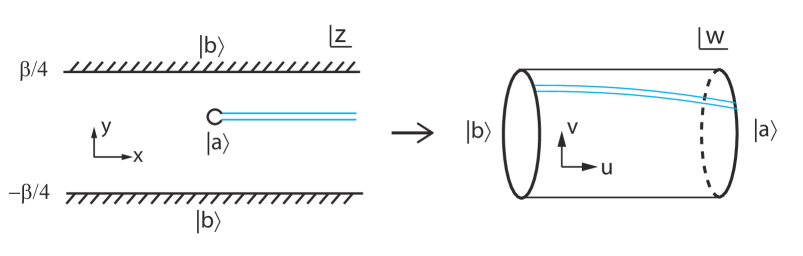
Figure 3: Euclidean spacetime for $\rho_{A}(\tau)$ after a global quantum quench, where the semi-infinite subsystem $A=[0,\infty)$ is part of the infinite real line. The width of the strip is $\beta/2$, and a branch cut (blue lines) is located along $C=\{i\tau+x,x\geq 0\}$. The fields living on the upper and lower edges of $C$ correspond to the rows and columns of $\rho_{A}$. We remove a small disc at the entangling surface $z_{0}=i\tau+0$ as regularization, and a conformal boundary state $|a\rangle$ is imposed along this disc. With the conformal mapping $w=f(z)$, the strip is mapped to an annulus, where the time slice $C$ is mapped to $f(C)$ which connects the two edges of the annulus, as shown in the right panel of the Figure. The circumference along the $v$-direction is $2\pi$.

Then the entanglement hamiltonian $K_{A}$, after the conformal mapping $w=f(z)$, can be considered as the generator of translation along the $v$ direction of the annulus. That is, it can be written in terms of the $vv$ component of the energy momentum tensor $T_{\mu\nu}$ as follows

$$K_{A}=-\int_{v=\text{const}}T_{vv}du=\int_{f(C)}T(w)dw+\int_{\overline{f(C)}}\overline{T}(\bar{w})d\bar{w},$$ (4)

where in the second step we introduce the holomorphic (antiholomorphic) component of the energy momentum tensor, $T$ ($\bar{T}$), and use the fact that $T_{00}=-T_{vv}=T+\overline{T}$ with the hamiltonian density $T_{00}$ in Minkowski signature and $T_{vv}$ in Euclidean signature. Upon mapping back to the $z$-plane, $K_{A}$ becomes

$$K_{A}=\int_{C}\frac{T(z)}{f^{\prime}(z)}dz+\int_{\overline{C}}\frac{\overline{T}(\bar{z})}{\overline{f^{\prime}(z)}}d\bar{z},$$ (5)

where the Schwartzian derivative term has been ignored since it will be canceled in the calculation of the entanglement entropy upon introducing the normalization factor $\text{Tr}\,\rho_{A}$. It is noted that the time slices $C$ and $\overline{C}$ in Eq. (5) do not coincide in the quantum quench case [29].

In particular, the entanglement hamiltonian for subsystem $A=[0,\infty)$ has at late times the approximate form

$$K_{A}(t)\simeq\frac{\beta}{2\pi}\int_{0}^{2t}T(x,t)dx,$$ (6)

where $T=(T_{00}+T_{10})/2$ is the energy-momentum tensor for only the right-movers, and involves both the hamiltonian density $T_{00}$ and the momentum density $T_{10}$. This result may be understood based on the quasi-particle picture in that only the right-moving quasiparticles in subsystem $A$ contribute to the entanglement (they are entangled with the left-moving ones in $B$).

The spectrum of $K_{A}(t)$ can also be obtained based on the knowledge of boundary CFT. The eigenvalues of $K_{A}$ are, up to a global shift, given by $\pi(\Delta_{j}-c/24)/W$ with degeneracies $d_{j}$ and central charge $c$. Here $\Delta_{j}$ are scaling dimensions of boundary operators. Then the spacing between levels of the entanglement spectrum may be expressed as

$$E_{i}-E_{j}=\frac{\pi(\Delta_{i}-\Delta_{j})}{W}.$$ (7)

It can be seen that the lowest eigenvalue $E_{0}$ has the form [29]

$$E_{0}\simeq\frac{c}{12}W+\log\langle a|0\rangle+\log\langle b|0\rangle.$$ (8)

To obtain the Renyi or von Neumann entropy, we need to evaluate the partition function $Z_{1}$ ($Z_{n}$) on the annulus in Fig.  3 below, with circumference $2\pi$ ($2n\pi$). It can be shown that, in the limit $W\gg 1$, one has

$$\frac{\text{Tr}(\rho_{A}^{n})}{(\text{Tr}\rho_{A})^{n}}=\frac{Z_{n}}{(Z_{1})^{n}}\simeq\frac{\langle a|0\rangle\langle 0|b\rangle\tilde{q}^{-c/24n}}{(\langle a|0\rangle\langle 0|b\rangle)^{n}\tilde{q}^{-cn/24}},\quad\text{with}\quad\tilde{q}=e^{-2W},$$ (9)

where $|0\rangle$ denotes the ground state of the CFT. Then one can obtain the Renyi entropy ($S^{(n)}_{A}$) and von Neumann entropy ($S_{A}$) as follows

$$S^{(n)}_{A}=\frac{1}{1-n}\frac{\text{Tr}(\rho_{A}^{n})}{(\text{Tr}\rho_{A})^{n}}\simeq\frac{c}{12}\left(1+\frac{1}{n}\right)W-g_{a}-g_{b},\quad S_{A}\simeq\frac{c}{6}W-g_{a}-g_{b},$$ (10)

where $g_{a,b}=-\log\langle a,b|0\rangle$ are the Affleck-Ludwig boundary entropies [38].

Observe the lack of thermalization in the entanglement hamiltonian (6), as it depends both on the hamiltonian and the momentum, which is due to the fact that $A$ is semi-infinite. Therefore, it is natural to ask the following questions: Can we study the time evolution of the entanglement hamiltonian for a finite subsystem during thermalization? If so, how does the entanglement spectrum evolve in time during this process? In particular, how does the entanglement spectrum converge to the saturated spectrum of a thermal ensemble in the long-time limit? Are there any quantities visualizing how the entanglement propagates, and how the subsystem is thermalized? To answer these questions, in this paper we are interested in the time evolution of the entanglement hamiltonian and related quantities for a finite interval, located at the end of a semi-infinite system, after a global quantum quench (see Fig.  1). The reason we choose this configuration is because in this case the corresponding path integral representation of the reduced density matrix can be mapped to an annulus and can then be treated analytically: Then one can use Cardy-Tonni’s approach to study analytically the behavior of entanglement hamiltonian/spectrum in this case.

2 Time evolution of entanglement hamiltonian

2.1 Conformal mapping

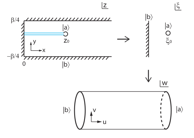
Figure 4: Euclidean spacetime for $\rho_{A}$ after a global quantum quench, where the finite interval $A=[0,L]$ is at the end of a semi-infinite system $A\cup B=[0,\infty)$. The width of the half-strip is $\beta/2$, and the branch cut (blue lines) is along $C=\{i\tau+x,0\leq x\leq L\}$. We remove a small disc at the entangling surface $z_{0}=i\tau+L$ as regularization. Conformal boundary conditions $|a\rangle$ and $|b\rangle$ are imposed, respectively, at the small circle at $z_{0}=i\tau+L$, and at the vertical and horizontal boundaries along $x=0$ and $y=\pm\frac{\beta}{4}$. The half strip is mapped to the right half plane (RHP) after the first conformal mapping $\xi=\xi(z)$, and further mapped to an annulus after the second conformal mapping $w=w(\xi)$. Here, we do not show explicitly the mapping of $C$ between the $\xi$- and the $z$-plane.

Shown in Fig.  4 is our setup for a global quantum quench in a semi-infinite system. As compared to the case in Fig.  3, we now have a physical boundary at position $x=0$, where we will impose a conformal boundary condition. In the space-(Euclidean)time picture of Fig.  4, this (spatial) boundary condition appears at the vertical boundary $0+iy$ ($-\beta/4\leq y\leq+\beta/4$). In general, this boundary condition can be different from the initial condition which is imposed in the space-(Euclidean)time picture of Fig.  4 at the horizontal boundary $x\pm i\beta/4$ ($0\leq x<\infty$), which is also represented (as mentioned) by a conformal boundary condition. When these two boundary conditions are different, one needs to consider boundary condition changing operators located at points where two different boundary conditions meet. For simplicity, we first assume that these two boundary conditions are the same, and we denote the corresponding conformal boundary state by $|b\rangle$. In addition, in order to take into account regularization, one removes a small disc at the entangling point located at $i\tau+L$, and imposes a conformal boundary condition $|a\rangle$ at the boundary of this (removed) disk (see Fig.  4).

It is noted that the Euclidean spacetime for this case is conformally equivalent to an annulus, and therefore one can use the method in Ref. [29]. As shown in Fig.  4, one can map the half strip in the $z$-plane (with the small disc at the entangling point $i\tau+L$ removed) to an annulus in the $w$-plane, by considering the following two-step conformal mapping $w=f(z)$,

$$\left\{\begin{split}\xi(z)=&\sinh\left(\frac{2\pi z}{\beta}\right),\\ w(\xi)=&-\log\left[\left(\frac{1+\overline{\xi}_{0}}{1+\xi_{0}}\right)\cdot\frac{\xi-\xi_{0}}{\xi+\overline{\xi}_{0}}\right],\end{split}\right.$$ (11)

where

$$\xi=\xi(z)\quad\text{and}\quad\xi_{0}=\xi(z_{0}),\quad\text{with}\quad z_{0}=i\tau+L.$$ (12)

The conformal mapping $\xi(z)$ in the first step maps the semi-infinite strip in the $z$-plane to the right half plane (RHP), namely $\rm{Re}(\xi)\geq 0$, in the $\xi$-plane (see Fig.  4). The small disc around the entangling surface $z_{0}=i\tau+L$ in the $z$-plane is mapped to a small disc around $\xi_{0}=\xi(z_{0})$ in the RHP. Then the second conformal mapping $w(\xi)$ sends the RHP with a small disc at $\xi_{0}$ removed to an annulus in the $w$-plane, where we write $w=u+iv$ with $u$ and $v$ real. After this two-step conformal mapping, the two boundaries labeled by $|a\rangle$ and $|b\rangle$ in the $z$-plane are mapped to the two boundaries (edges) of the annulus in the $w$-plane, described by $\{u=f(i\tau+\epsilon),0\leq v<2\pi\}$ and $\{u=f(i\tau+L-\epsilon),0\leq v<2\pi\}$, respectively. In Fig.   5 we show the constant-$u$ and constant-$v$ flows in the $z$-plane and the $w$-plane, respectively. In particular, in the $w$-plane, these are straight lines, where $u$ runs from $f(\epsilon+i\tau)$ to $f(L-\epsilon+i\tau)$, and $v$ runs from $-\pi$ to $\pi$. In the path integral description of $\text{Tr}\,\rho_{A}$, the two segments along $v=-\pi$ and $v=\pi$ are identified.

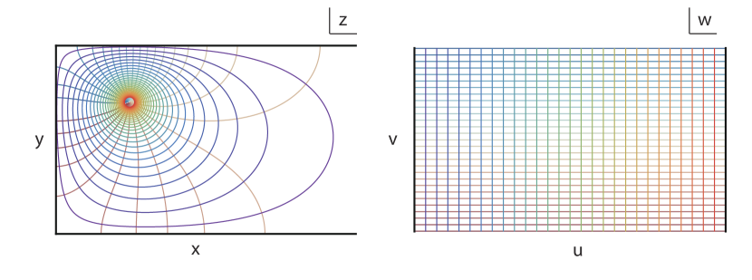
Figure 5: Euclidean spacetime for a global quench of a semi-infinite system, where $A=[0,L]$ and $A\cup B=[0,\infty)$. The vertical width of the half strip is $\beta/2$. The curves in the $z$-plane in the left panel correspond to constant-$u$ and constant-$v$ curves in the $w$-plane in the right panel, with $w=u+iv$, and $v\in[-\pi,\pi)$.

2.2 Time evolution of entanglement hamiltonian

2.2.1 Entanglement hamiltonian for subsystem $[0,L]$

 

Based on Eq. (5) and the conformal mapping in Eq. (11), it is straightforward to obtain the entanglement hamiltonian $K_{A}(t)$ for subsystem $A$ as follows (after analytical continuation $\tau\to it$):

$$\begin{split}K_{A}(t)=&\frac{\beta}{\pi}\int_{L}^{0}\frac{\sinh\left[\frac{\pi(x-L)}{\beta}\right]\cosh\left[\frac{\pi\left(x-2t+L\right)}{\beta}\right]\sinh\left[\frac{\pi(x+L)}{\beta}\right]\cosh\left[\frac{\pi(x-2t-L)}{\beta}\right]}{\cosh\left(\frac{2\pi}{\beta}t\right)\sinh\left(\frac{2\pi}{\beta}L\right)\cosh\left[\frac{2\pi}{\beta}\left(x-t\right)\right]}T(x,t)dx\\ \rule{0.0pt}{22.76228pt}&+\frac{\beta}{\pi}\int_{L}^{0}\frac{\sinh\left[\frac{\pi(x-L)}{\beta}\right]\cosh\left[\frac{\pi\left(x+2t+L\right)}{\beta}\right]\sinh\left[\frac{\pi(x+L)}{\beta}\right]\cosh\left[\frac{\pi(x+2t-L)}{\beta}\right]}{\cosh\left(\frac{2\pi t}{\beta}\right)\sinh\left(\frac{2\pi L}{\beta}\right)\cosh\left[\frac{2\pi\left(x+t\right)}{\beta}\right]}\overline{T}(x,t)dx.\end{split}$$ (13)

Let us check the behavior of $K_{A}(t)$ at $t=0$ first. There are the following two interesting cases:

(i) $t=0,\beta\to\infty$. In this case, the width of the strip in Fig.  4 goes to infinity, and the initial state at $t=0$ is no longer a short-range entangled state. It corresponds to the ground state of a CFT with a physical boundary at $x=0$. After some simple algebra, Eq. (13) can be simplified to

$$K_{A}(t=0,\beta\to\infty)\simeq\int_{0}^{L}\frac{L^{2}-x^{2}}{2L}T_{00}(x)dx,$$ (14)

which agrees with the (known) result for the entanglement hamiltonian of a finite interval at the end of a semi-infinite CFT.

(ii) $t=0,L\gg\beta$. In this case, $L$ is much larger than the correlation length of the initial state. It is straightforward to find that

$$K_{A}(t=0,L\gg\beta)= \frac{\beta}{2\pi}\int_{0}^{L}\sinh\left[\frac{2\pi}{\beta}(L-x)\right]T_{00}(x)dx.$$ (15)

Here, the contribution to the entanglement between $A$ and $B$ mainly comes from the region near the entangling point, i.e., $(L-x)\sim\mathcal{O}(\beta)$, as appropriate for a short-range entangled state. For $(L-x)\gg\beta$, the entanglement hamiltonian becomes exponentially large, and its contribution to the entanglement becomes exponentially suppressed, as expected.

Now let us focus on the time evolution of $K_{A}(t)$ for $t>0$. $K_{A}(t)$ shows different behaviors in different time-regimes: (See Appendix A for details.)

$$K_{A}(t)\simeq\left\{\begin{split}&\frac{\beta}{2\pi}\int_{L-2t}^{L}\overline{T}(x,t)dx,\quad&t<L/2,\\ &\frac{\beta}{2\pi}\int_{0}^{2t-L}T_{00}(x,t)dx+\frac{\beta}{2\pi}\int_{2t-L}^{L}\overline{T}(x,t)dx,\quad&L/2<t<L,\\ &\frac{\beta}{2\pi}\int_{0}^{L}T_{00}(x,t)dx,\quad&t>L.\end{split}\right.$$ (16)

Here we have ignored the interesting contributions close to the entangling point, i.e., contributions coming from regions $L-x\sim O(\beta)$ [see Eqs. (49)-(52) in Appendix]. $T$, $\overline{T}$ and $T_{00}$ are related via $T=(T_{00}+T_{10})/2$ and $\overline{T}=(T_{00}-T_{10})/2$, where $T$ ($\overline{T}$) is the energy-momentum tensor for the right (left) movers. The behavior of $K_{A}(t)$ in Eq. (16) may be understood as follows:

(i) $t<L/2$. Only the energy momentum tensor for the left movers, namely $\overline{T}(x,t)$, appears in $K_{A}(t)$. This can be easily understood based on Fig.  2(a), where only the left-moving quasiparticles in interval $A$ contribute to the entanglement between $A$ and $B$. In particular, these quasiparticles are distributed in subinterval $[L-2t,L]$, corresponding to the integral $\int_{L-2t}^{L}\cdots dx$ in the expression for $K_{A}(t<L/2)$ in Eq. (16).

(ii) $L/2<t<L$. Here, $K_{A}(t)$ can be rewritten as

$$\begin{split}K_{A}\left(L/2<t<L\right)\simeq\frac{\beta}{2\pi}\int_{0}^{2t-L}T(x,t)dx+\frac{\beta}{2\pi}\int_{0}^{L}\overline{T}(x,t)dx.\end{split}$$ (17)

That is, the right movers $T(x,t)$ start to contribute to $K_{A}(t)$. The intervals over which the corresponding integrals extend, i.e. $\int_{0}^{2t-L}T(x,t)dx$ and $\int_{0}^{L}\overline{T}(x,t)dx$ respectively, also agree with the physical picture in Fig.  2 (b) which says that the right-moving quasiparticles in $[0,2t-L]$ and the left-moving quasiparticles in $[0,L]$ contribute to the entanglement between $A$ and $B$.

(iii) $t>L$. Only the hamiltonian density $T_{00}(x,t)$ appears in $K_{A}(t)$. Considering that $T_{00}(x,t)=T(x,t)+\overline{T}(x,t)$, the term proportional to $\int_{0}^{L}T_{00}(x,t)dx$ agrees with the physical picture in Fig.  2 (c) which says that both the left-moving and right-moving quasiparticles distributed in $[0,L]$ contribute to the entanglement.

Note that we have ignored the contributions near the entangling point when evaluating $K_{A}(t)$ in Eq. (16). In particular, in the long time limit $t\to\infty$, one obtains the following expression when keeping all contributions

$$K_{A}(t\to\infty)=\frac{\beta}{\pi}\int_{0}^{L}\frac{\sinh[\pi(L-x)/\beta]\sinh[\pi(L+x)/\beta]}{\sinh(2\pi L/\beta)}T_{00}(x,t)dx,$$ (18)

which has the same form as that of the entanglement hamiltonian in the thermal ensemble [see Eq. (67)]. In fact, as shown below, for $t\to\infty$ the spectrum of $K_{A}(t)$ is exactly the same as that in the thermal ensemble. This indicates that in the long time limit $t\to\infty$ the reduced density matrix $\rho_{A}(t)$ is exactly the same as the reduced density matrix $\rho_{A}(\beta)$ in the thermal ensemble at finite temperature $\beta^{-1}$.

2.2.2 Entanglement hamiltonian for subsystem $(L,\infty)$

 

To obtain the entanglement hamiltonian $K_{B}(t)$ for subsystem $B=(L,\infty)$, we simply need to replace the path $C=\{i\tau+x,0\leq x\leq L\}$ with the path $C=\{i\tau+x,x>L\}$ in Eq. (5) [see also Fig.  4], and therefore change the interval over which the integral in Eq. (13) is taken, from $\int_{L}^{0}\cdots dx\to\int_{L}^{\infty}\cdots dx$. After some simple algebra, one finds

$$K_{B}(t)\simeq\left\{\begin{split}&\frac{\beta}{2\pi}\int_{L}^{2t+L}T(x,t)dx,\quad t<L,\\ &\frac{\beta}{2\pi}\int_{2t-L}^{2t+L}T(x,t)dx,\quad t>L,\end{split}\right.$$ (19)

where, again, we have ignored the contributions close to the entangling point, i.e. from the region $x-L\sim O(\beta)$. One interesting feature in the expressions for $K_{B}(t)$ above is that only the energy momentum tensor for the right movers, namely $T(x,t)$, appears in $K_{B}(t)$. This can be easily understood based on the quasi-particle picture in Fig. 2, where only the right movers distributed in $[L,2t+L]$ for $t<L$ (and distributed in $[2t-L,2t+L]$ for $t>L$) in subsystem $B$ contribute to the entanglement between $B$ and $A$. We emphasize the difference between Eq. (19), and Eq. (6) valid for subsystem $[0,\infty)$ in the infinite system $(-\infty,\infty)$ [29]. For $t<L$, the result in Eq. (19) agrees with Eq. (6) by setting $L=0$. For $t>L$, however, the interval over which the integral in Eq. (19) is taken is $[2t-L,2t+L]$ with a constant width $2L$, which is different from the interval $[0,2t]$ appearing in Eq. (6) which grows linearly in $t$. This is because the reservoir for the entanglement Hamiltonian in Eq. (19) for region $B=[L,\infty)$ is region $A=[0,L]$ which is finite, while the reservoir of the entanglement hamiltonian in Eq. (6) for region $A=[0,\infty)$ is region $B=(-\infty,0)$, which is infinite.

In addition, note that in the long time limit $t\to\infty$, the entanglement hamiltonian $K_{B}(t)$ in Eq. (19) can never approach that in a thermal ensemble. In other words, subsystem $B$ can not thermalize, because it is of infinite spatial extent.

3 Time evolution of entanglement spectrum and entanglement entropy

Here we use the method briefly reviewed in Sec. 1.4 to study the time evolution of the entanglement spectrum and of the entanglement entropy. By defining

$$\mathcal{W}=f(i\tau+L-\epsilon)-f(i\tau),$$ (20)

where $f(z)$ is the conformal mapping in Eq. (11), the width $W$ of the annulus (see Fig. 4) can be expressed as

$$W=\text{Re}(\mathcal{W})=\frac{1}{2}\left(\mathcal{W}+\overline{\mathcal{W}}\right).$$ (21)

After some straightforward algebra, one finds that $\mathcal{W}$ has the explicit form

$$\mathcal{W}=\log\left\{\frac{\cosh\left[\frac{2\pi}{\beta}\cdot\frac{i2\tau+L}{2}\right]}{\cosh\left[\frac{2\pi}{\beta}\cdot\frac{i2\tau-L}{2}\right]}\cdot\frac{\sinh\left(\frac{2\pi}{\beta}\cdot\frac{2L-\epsilon}{2}\right)\cdot\cosh\left(\frac{2\pi}{\beta}\cdot\frac{i2\tau-\epsilon}{2}\right)}{\sinh\left(\frac{2\pi}{\beta}\cdot\frac{\epsilon}{2}\right)\cdot\cosh\left(\frac{2\pi}{\beta}\cdot\frac{i2\tau+2L-\epsilon}{2}\right)}\right\}.$$ (22)

Upon analytical continuation to real time, $\tau\to it$, one obtains

$$W=\frac{1}{2}(\mathcal{W}+\overline{\mathcal{W}})=\log\left\{\frac{2\sinh\left[\frac{2\pi}{\beta}(L-\frac{\epsilon}{2})\right]\cdot\cosh\left(\frac{2\pi t}{\beta}\right)}{\sinh\left(\frac{2\pi}{\beta}\cdot\frac{\epsilon}{2}\right)\cdot\sqrt{2\cosh\left(\frac{2\pi}{\beta}\cdot 2L\right)+2\cosh\left(\frac{2\pi}{\beta}\cdot 2t\right)}}\right\}.$$ (23)

By further considering the limit $L,t\gg\beta\gg\epsilon$, this expression for $W$ can be simplified as

$$W\simeq\left\{\begin{split}&\log\left(\frac{\beta}{2\pi\epsilon}\right)+\frac{2\pi}{\beta}t,\quad&t<L,\\ &\log\left(\frac{\beta}{2\pi\epsilon}\right)+\frac{2\pi}{\beta}L,\quad&t>L,\end{split}\right.\quad\Rightarrow\quad S_{A}(t)\simeq\left\{\begin{split}&\frac{\pi c}{3\beta}t,\quad&t<L,\\ &\frac{\pi c}{3\beta}L,\quad&t>L,\end{split}\right.$$ (24)

where in the second step we have used Eq. (10), and have only kept the leading term in $t$ or $L$. For $t<L$, $S_{A}\simeq(\pi c/3\beta)t$, i.e., the entanglement entropy grows linearly in time. For $t>L$, both $W$ and the entanglement entropy $S_{A}(t)$ are saturated. They are the same as those displayed in Eqs. (65) and (66) for the thermal ensemble, to leading order in large quantities.

As just mentioned, the results in Eq. (24) are approximated in that only the leading order in $t$ or $L$ has been kept. In fact, in the limit $t\to\infty$, one can find the exact expression of $W$ based on Eq. (23), which reads as follows

$$W(t\to\infty)=\log\frac{\sinh[\pi(2L-\epsilon)/\beta]}{\sinh(\pi\epsilon/\beta)}=:W_{\text{thermal}}.$$ (25)

This expression is exactly the same as that for the thermal ensemble, displayed in Eq. (64), indicating that the long time limit of the reduced density matrix $\rho_{A}(t\to\infty)$ is indistinguishable from the reduced density matrix in the thermal ensemble at finite temperature $\beta^{-1}$. Then the level spacing of the entanglement spectrum has the following form

$$E_{i}-E_{j}=\frac{\pi(\Delta_{i}-\Delta_{j})}{W_{\text{thermal}}},\quad\text{with }t\to\infty.$$ (26)

It is interesting to check how the width $W(t)$ in Eq. (23) approaches the saturated long time value $W_{\text{thermal}}$ as a function of time. For $t-L\gg\beta$, by expanding $W$ to the term in $t$, it is straightforward to obtain

$$W(t>L)\simeq W_{\text{thermal}}-\frac{1}{2}e^{-\frac{4\pi}{\beta}(t-L)}.$$ (27)

Therefore, for $t-L\gg\beta$, one obtains the following behavior of the spacing of the entanglement spectrum

$$E_{i}(t)-E_{j}(t)=\frac{\pi(\Delta_{i}-\Delta_{j})}{W}\simeq\frac{\pi(\Delta_{i}-\Delta_{j})}{W_{\text{thermal}}}\left[1+\frac{1}{2W_{\text{thermal}}}e^{-\frac{4\pi}{\beta}(t-L)}\right],\quad\text{with }t-L\gg\beta.$$ (28)

That is, the spacing of the entanglement spectrum converges exponentially in time to its saturated long time value $\pi(\Delta_{i}-\Delta_{j})/W_{\text{thermal}}$.

It is also worth checking the behavior of $\mathcal{W}$ and $\overline{\mathcal{W}}$ respectively after analytical continuation $\tau\to it$. In the region $t<L/2$, based on Eq. (22) and its complex conjugate $\overline{\mathcal{W}}$, one has

$$\left\{\begin{split}\mathcal{W}|_{\tau=it}&\simeq\log\left(\frac{\beta}{2\pi\epsilon}\right),\\ \overline{\mathcal{W}}|_{\tau=it}&\simeq\log\left(\frac{\beta}{2\pi\epsilon}\right)+\frac{2\pi}{\beta}\cdot 2t.\\ \end{split}\right.$$ (29)

The entanglement entropy mainly comes from $\overline{\mathcal{W}}|_{\tau=it}$, i.e., from the left movers. This agrees with Eq. (16) which says that only the left movers $\overline{T}(x,t)$ appear in the entanglement hamiltonian $K_{A}(t<L/2)$. It is remarkable that the factor $2t$ in the expression for $\overline{W}|_{\tau\to it}$ corresponds to the length of the interval $[L-2t,L]$ for the left-moving quasiparticles in Fig.  2(a).

In the region $L/2<t<L$, one obtains

$$\left\{\begin{split}\mathcal{W}|_{\tau=it}&\simeq\log\left(\frac{\beta}{2\pi\epsilon}\right)+\frac{2\pi}{\beta}(2t-L),\\ \overline{\mathcal{W}}|_{\tau=it}&\simeq\log\left(\frac{\beta}{2\pi\epsilon}\right)+\frac{2\pi}{\beta}L.\\ \end{split}\right.$$ (30)

Now, both $\mathcal{W}|_{\tau\to it}$ and $\overline{\mathcal{W}}|_{\tau\to it}$ contribute to the entanglement entropy $S_{A}(t)$. In particular, the factor $(2t-L)$ in the expression for $\mathcal{W}|_{\tau\to it}$ corresponds to the length of the interval $[0,2t-L]$ occupied by the right-moving quasiparticles, and the factor $L$ in the expression for $\overline{\mathcal{W}}|_{\tau\to it}$ corresponds to the length of the interval $[0,L]$ for the left-moving quasiparticles in Fig.  2(b).

For $t>L$, one obtains

$$\left\{\begin{split}\mathcal{W}|_{\tau=it}&\simeq\log\left(\frac{\beta}{2\pi\epsilon}\right)+\frac{2\pi}{\beta}L,\\ \overline{\mathcal{W}}|_{\tau=it}&\simeq\log\left(\frac{\beta}{2\pi\epsilon}\right)+\frac{2\pi}{\beta}L.\\ \end{split}\right.$$ (31)

The contributions of $\mathcal{W}|_{\tau\to it}$ and $\overline{\mathcal{W}}|_{\tau\to it}$ to the entanglement entropy $S_{A}(t)$ are the same. The factor $L$ in $\mathcal{W}|_{\tau\to it}$ and $\overline{\mathcal{W}}|_{\tau\to it}$ agrees with the length of $[0,L]$ which is occupied by both left-moving and right-moving quasiparticles in Fig.  2(c).

4 Modular flows in Minkowski spacetime

In this section, we study the modular flow, the fictitious real-time-evolution generated by the entanglement hamiltonian; it is represented by a (Killing) vector field in Minkowski spacetime. In terms of the $w$-coordinate, this is the flow generated by keeping $u$ constant and varying $v$. Our motivation to study the constant-$u$ flows is very straightforward: In the previous part, we have seen that the entanglement entropy $S_{A}$ is proportional to the width $W$ of annulus in the $w$-plane [see Eq. (10)]. Note that $W$ measures the range of the variable $u=\text{Re}\,w$ in the $w$-plane. Therefore, the constant-$u$ flows with $u_{\text{max}}-u_{\text{min}}=W$ should provide us information about the entanglement between $A$ and $B$. Moreover, in Sec.2, we have seen that the time evolution of the entanglement entropy and entanglement hamiltonian can be well understood in terms of the quasi-particle picture. Based on the above observations, we expect there should be a correspondence between the patterns of modular flows and the quasi-particle picture, as studied in detail in the following.

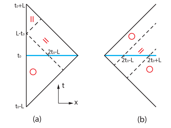
Figure 6: (a) Causal wedge for subsystem $A=\{(x,t_{0}),0\leq x\leq L\}$ (blue solid line) with $t_{0}<L$ in Minkowski spacetime, with a physical boundary along $x=0$. The wedge is divided into three regions labeled by $|\,|$, $\backslash\backslash$, and $\bigcirc$, respectively, as defined in Eqs. (32) and (33). (b) Causal wedge for subsystem $B=\{(x,t_{0}),L<x<\infty\}$ with $t_{0}>L$. The wedge is divided into two regions $//$ and $\bigcirc$, as defined in Eqs. (37) and (38).

4.1 Flows in Minkowski spacetime for subsystem $[0,L]$

Shown in Fig.  6 (a) is the causal wedge for subsystem $A=[0,L]$ at $t_{0}$. Here we denote by $t_{0}$ the observation time, and by $t$ the Minkowski coordinate. To facilitate our later discussion, we divide the causal wedge into three regions labeled by symbols $|\,|$, $\backslash\backslash$, and $\bigcirc$ as follows:

$$\text{region }|\,|:\quad\left\{\begin{split}&t-(L-t_{0})>x,\\ &t-(L+t_{0})<-x,\\ &x>0,\end{split}\right.\quad\text{region }\backslash\backslash:\quad\left\{\begin{split}&t-(L-t_{0})<x,\\ &t-(L-t_{0})>-x,\\ &t-(L+t_{0})<-x,\\ &t-(t_{0}-L)>x,\end{split}\right.$$ (32)

and

$$\text{region }\bigcirc:\quad\left\{\begin{split}&t-(L-t_{0})<x,\\ &t-(L-t_{0})<-x,\\ &t-(t_{0}-L)>x,\\ &t-(t_{0}-L)>-x.\end{split}\right.$$ (33)

It is noted that these regions are well defined for $t_{0}\leq L$. For $t_{0}>L$, regions $\backslash\backslash$ and $\bigcirc$ will shrink to zero, and region $|\,|$ will occupy the whole wedge.

Given the conformal mapping $w=f(z)$ in Eq. (11), and by considering $\text{Re}f(z)=u$ and making the analytic continuation $\tau\to it$, one obtains the equation describing these flows (compare also Eq.s (74,75,76) in Appendix B):

$$\begin{split}&\frac{\cosh\frac{2\pi}{\beta}\left(x-L\right)-\cosh\frac{2\pi}{\beta}\left(t-t_{0}\right)}{\cosh\frac{2\pi}{\beta}\left(x+L\right)-\cosh\frac{2\pi}{\beta}\left(t-t_{0}\right)}\cdot\frac{\cosh\frac{2\pi}{\beta}\left(x+L\right)+\cosh\frac{2\pi}{\beta}\left(t+t_{0}\right)}{\cosh\frac{2\pi}{\beta}\left(x-L\right)+\cosh\frac{2\pi}{\beta}\left(t+t_{0}\right)}=e^{-2u}.\end{split}$$ (34)

Based on this equation, we plot the constant-$u$ flows in Fig.  7. One finds that the result depends on the observation time $t_{0}$. We note the following interesting features:

(i) For $t_{0}<L$, one can always observe the three different regions labeled by $|\,|$, $\backslash\backslash$, and $\bigcirc$ in Fig.  6. In particular, region $|\,|$ is filled with vertical flows, region $\backslash\backslash$ is filled with left-tilted flows, and region $\bigcirc$ is empty (no flows).

(ii) As the observation time $t_{0}$ increases, regions $\backslash\backslash$ and $\bigcirc$ gradually shrink to zero, and the region $|\,|$ of vertical flows gradually increases until $t_{0}=L$. For $t_{0}\geq L$, the whole wedge is occupied by vertical flows, and the distribution of these vertical flows is independent of $t_{0}$. Upon comparing with Fig.  14 for a finite interval $[0,L]$ at the end of a semi-infinite system at finite temperature $\beta^{-1}$, one observes that the distributions of vertical flows are the same (See also Ref. [41] for the modular flows in a thermal ensemble.). This indicates that subsystem $A$ in Fig.  7 is thermalized for $t_{0}>L$.

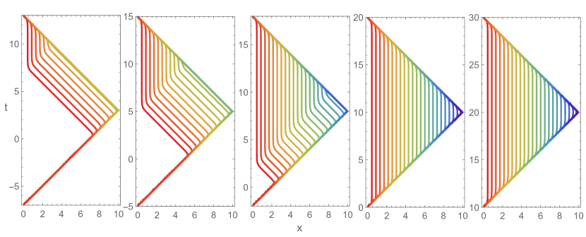
Figure 7: Constant-$u$ flows in the causal wedge of subsystem $A=\{(x,t_{0}),0\leq x\leq L\}$ in Minkowski spacetime, plotted according to Eq. (34). The parameters we use are $\beta=1.5$, and $L=10$. The observation times are $t_{0}=3,5,8,10,20$ from left to right. Region $|\,|$ (see the definition in Fig.  6) is occupied by vertical flows, region $\backslash\backslash$ is occupied by left-tilted flows, and region $\bigcirc$ is occupied by nothing. As time $t_{0}$ increases, the causal wedge is gradually occupied by region $|\,|$. For $t_{0}>L$, the causal wedge is totally occupied by region $|\,|$ with vertical flows, which are independent of the observation time $t_{0}$. See Eq. (36) for more quantitative interpretation.

Furthermore, as shown in Appendix A.2, the flows in region $|\,|$ and region $\backslash\backslash$ can be approximately described by

$$\left\{\begin{split}&\text{flows in region }|\,|:\quad x=\frac{\beta}{2\pi}u,\\ &\text{flows in region }\backslash\backslash:\quad(x-L)+(t+t_{0})=\frac{\beta}{\pi}u.\end{split}\right.$$ (35)

It is noted that the vertical flows described by $x=\beta u/2\pi$ are the feature of a thermal ensemble [41]. It agrees with Eq. (72) for a thermal ensemble at temperature $\beta^{-1}$, up to a global constant shift. On the other hand, left- (and right-) tilted constant-$u$ flows are a feature of a global quench without thermalization, as shown in Fig. 15 in Appendix. The second equation in Eq. (35) agrees (up to a global constant shift) with Eq. (80) describing a semi-infinite subsystem $A$ after a quantum quench.

Therefore, the time evolution of the constant-$u$ flows in Fig.  7 shows how subsystem $A$ is thermalized as $t_{0}$ increases. Furthermore, we can obtain a quantitative correspondence between the flows in Fig.  7 and the entanglement hamiltonian $K_{A}(t)$ in Eq. (16). By simply looking at which kind of region intersects subsystem $A=\{(x,t_{0}),0\leq x\leq L\}$, one finds

$$\begin{split}(i)\,\,t_{0}<L/2:\quad\backslash\backslash\cap A&=[L-2t_{0},L]\longleftrightarrow\int_{L-2t_{0}}^{L}\overline{T}(x,t_{0})dx.\\ (ii)\,\,L/2<t_{0}<L:\quad|\,|\cap A&=[0,2t_{0}-L]\longleftrightarrow\int_{0}^{2t_{0}-L}T_{00}(x,t_{0})dx.\\ \backslash\backslash\cap A&=[2t_{0}-L,L]\longleftrightarrow\int_{2t_{0}-L}^{L}\overline{T}(x,t_{0})dx.\\ (iii)\,\,t_{0}>L:\quad|\,|\cap A&=[0,L]\longleftrightarrow\int_{0}^{L}T_{00}(x,t_{0})dx.\end{split}$$ (36)

Based on this quantitative correspondence, we can conclude that the left-tilted flows in region $\backslash\backslash$ are contributed by the left-moving quasiparticles, and the vertical flows in region $|\,|$ are contributed by both left-moving and right-moving quasiparticles.

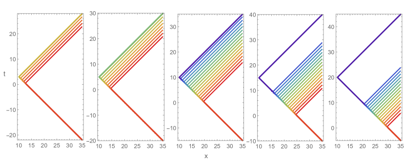
Figure 8: Constant-$u$ flows in the causal wedge of subsystem $B=\{(x,t_{0}),L<x<\infty\}$ in Minkowski spacetime, plotted according to Eq. (34). The parameters we use are $\beta=1.5$, and $L=10$. From left to right, we have $t_{0}=3,5,10,15,20$. For $t_{0}<L$, region $//$ (see the definition in Eqs.(37) and (38)), which is filled with right-tilted flows, grows as a function of $t_{0}$. For $t_{0}>L$, region $//$ does not grow any more, but simply moves rightwards. See Eq. (40) for more interpretation.

4.2 Flows in Minkowski spacetime for subsystem $(L,\infty)$

Now we consider the causal wedge for $B=\{(x,t_{0}),L<x<\infty\}$, as shown in Fig.  6 (b). We divide the wedge into two regions, region $//$ (which is filled with right-tilted flows) and the remaining part (labeled by the symbol $\bigcirc$). Region $//$ is defined as

$$\text{region }//:\left\{\begin{split}&t-t_{0}<x-L,\\ &t-t_{0}>-(x-L),\\ &t-t_{0}>x-(2t_{0}+L),\end{split}\right.\quad\text{for }t_{0}<L,$$ (37)

and

$$\text{region }//:\left\{\begin{split}&t-t_{0}<x-(2t_{0}-L),\\ &t-t_{0}>-(x-L),\\ &t-t_{0}>x-(2t_{0}+L),\end{split}\right.\quad\text{for }t_{0}>L.$$ (38)

The corresponding constant-$u$ flows in Minkowski spacetime are shown in Fig.  8. There are several interesting features:

(i) For $t_{0}<L$, the region $//$ which is filled with right-tilted flows grows as a function of $t_{0}$.

(ii) For $t_{0}>L$, region $//$ does not grow any more as $t_{0}$ increases, but simply moves rightwards linearly in $t_{0}$. For comparison, we study the constant-$u$ flows for the region $A=[0,\infty]$ in an infinite system $(-\infty,+\infty)$ after a global quench. As shown Fig.  15, the region $//$ always grows as a function of time $t_{0}$, and never saturates. This difference arises from the following facts: For the case in Fig.  8, the number of quasiparticles carrying entanglement in $(L,\infty)$ will saturate due to the finite size of its reservoir $[0,L]$. For the case in Fig.  15, due to the semi-infinite size of both, of subsystem $A=[0,\infty)$ as well as of the reservoir $B=(-\infty,0)$, the number of quasiparticles carrying entanglement in $A$ will continue to grow as a function of time $t_{0}$ without saturation. This agrees with the analysis given in the paragraph below Eq. (19).

(iii) When compared with Fig.  7, there are no vertical flows in Fig.  8. This is because there are only right-moving quasiparticles carrying entanglement in region $(L,\infty)$.

In addition, as shown in the appendix, the flows in region $//$ can be approximately described by

$$\text{flows in region }//:\quad(x-L)-(t+t_{0})=-\frac{\beta}{\pi}u.$$ (39)

Again, this is a feature of a global quantum quench without thermalization. It agrees (up to a global constant shift) with Eq. (78), which describes the right-tilted flows for subsystem $A=[0,\infty)$ in an infinite system $(-\infty,+\infty)$ after a global quantum quench.

Similarly, one can find the following quantitative correspondence between the constant-$u$ flows and the entanglement hamiltonian,

$$\begin{split}(i)\,\,t_{0}<L:\quad//\cap B&=[L,2t_{0}+L]\longleftrightarrow\int_{L}^{2t_{0}+L}T(x,t_{0})dx.\\ (ii)\,\,t_{0}>L:\quad//\cap B&=[2t_{0}-L,2t_{0}+L]\longleftrightarrow\int_{2t_{0}-L}^{2t_{0}+L}T(x,t_{0})dx,\end{split}$$ (40)

where $T(x,t_{0})$ is the energy-momentum tensor for the right movers. Based on the above analysis, one sees that the right-tilted flows in region $//$ are contributed by the right-moving quasiparticles.

In short, for the flows in Fig.  7 and Fig.  8, we find that the left-tilted flows in region $\backslash\backslash$ and right-tilted flows in region $//$ are contributed by the left-moving and right-moving quasiparticles, respectively. The vertical flows in region $|\,|$ are contributed by the left-moving and the right-moving quasiparticles. In region $\bigcirc$, there are no flows, and no quasiparticles in this region can contribute to entanglement. The correspondence among the constant-$u$ flows, quasiparticles (q.p.) carrying entanglement, and the entanglement hamiltonians can be summarized as

$$\left\{\begin{split}\text{vertical flows in region }|\,|&\Leftrightarrow\text{left}+\text{right-moving q.p.}\Leftrightarrow\int T_{00}(x,t)dx\\ \text{left-tilted flows in region }\backslash\backslash&\Leftrightarrow\text{left-moving q.p.}\Leftrightarrow\int\overline{T}(x,t)dx\\ \text{right-tilted flows in region }//&\Leftrightarrow\text{right-moving q.p.}\Leftrightarrow\int T(x,t)dx.\\ \end{split}\right.$$ (41)

The time evolution of the entanglement hamiltonian and the modular flows in Minkowski spacetime provide us with an intuitive picture on how the entanglement propagates, and how the subsystem thermalizes.

5 Discussion of generic initial states

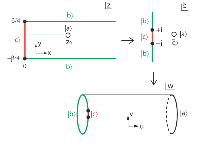
Figure 9: Setup for a global quantum quench with $|b\rangle\neq|c\rangle$. With the same conformal mapping in Eq. (11), the half-rectangle can be mapped to an annulus in the $w$-plane. The black dots represent boundary condition changing operators.

Here, by a generic initial state, we mean an initial state described by $|\phi_{0}\rangle=e^{-(\beta/4)H_{\rm{CFT}}}|b\rangle$ corresponding to a regularized version of a conformal boundary state $|b\rangle$, which may be different from the conformal boundary state $|c\rangle$ describing the physical boundary condition at position $x=0$ (the left end of the semi-infinite region $[0,+\infty)$), as shown in Fig.9. When $|b\rangle\not=|c\rangle$, the form of the entanglement hamiltonian and of the modular flows is the same as in the case where $|b\rangle=|c\rangle$. However, one should be more careful about the boundary condition(s) on the left edge of the annulus in the $w$-plane (see Fig.9), which may affect the spectrum of the entanglement hamiltonian. In the following, we will analyze how this boundary condition evolves as a function of time after a quantum quench.

Let us focus on the boundary along $z\in\left\{x\pm i\frac{\beta}{4}:x\geq 0\right\}\cup\left\{0+iy:-\beta/4\leq y\leq\beta/4\right\}$ in the $z$-plane (Fig.9): The conformal boundary condition $|b\rangle$ is imposed along the horizontal boundaries $z=\left(x\pm i\frac{\beta}{4}\right)$, $x>0$, while the boundary condition $|c\rangle$ is imposed along the vertical boundary $z=\left(0+iy\right)$, $-\beta/4<y<+\beta/4$. With the two-step conformal mapping in Eq. (11), the entire boundary (consisting of horizontal and vertical pieces) is mapped to the left edge of annulus in the $w$-plane, which is a circle with circumference $2\pi$. It is straightforward to check that this circle is along $\text{Re}\,w=0$ in the $w$-plane. Now we are mainly interested in where the two boundary conditions $|b\rangle$ and $|c\rangle$ are located along this circle. Without loss of generality, let us study the location of the boundary condition $|b\rangle$ (boundary condition $|c\rangle$ is located in the remaining interval of the circle, the complement), which is defined along

$$w\left(x\pm i\frac{\beta}{4}\right)=-\log\left\{\frac{1+\sinh\left[\frac{2\pi}{\beta}(-i\tau+L)\right]}{1+\sinh\left[\frac{2\pi}{\beta}(i\tau+L)\right]}\cdot\frac{\sinh\left[\frac{2\pi}{\beta}(x\pm i\frac{\beta}{4})\right]-\sinh\left[\frac{2\pi}{\beta}(i\tau+L)\right]}{\sinh\left[\frac{2\pi}{\beta}(x\pm i\frac{\beta}{4})\right]+\sinh\left[\frac{2\pi}{\beta}(-i\tau+L)\right]}\right\},$$ (42)

where $x\geq 0$. As shown in Fig.10, we use the following quantity to characterize how $|b\rangle$ wraps around the circle along $\text{Re}\,w=0$:

$$\alpha(x):=w\left(x+i\frac{\beta}{4}\right)-w\left(x-i\frac{\beta}{4}\right).$$ (43)

After some algebra, and upon making the analytical continuation $\tau\to it$, one obtains

$$\alpha(x)=2\,\text{arctan}\left(\frac{4\cosh\frac{2\pi t}{\beta}\sinh\frac{2\pi L}{\beta}\cosh\frac{2\pi x}{\beta}}{\cosh\frac{4\pi L}{\beta}-\cosh\frac{4\pi t}{\beta}-2\cosh^{2}\frac{2\pi x}{\beta}}\right).$$ (44)

The location of the boundary condition $|b\rangle$ as well as its effect on the entanglement spectrum may be discussed in the following two time regimes:

Figure 10: Location of boundary conditions $|b\rangle$ and $|c\rangle$ on the left edge of the annulus in the $w$-plane, with $w=u+iv$ (see Fig.9). For $t<L$, the edge is dominated by the conformal boundary condition $|b\rangle$. For $t>L$, half the edge has boundary condition $|b\rangle$, and the other half has boundary condition $|c\rangle$.

(i) $t<L$

Here, we are interested in the case $L-t\gg O(\beta)$. In this time regime, the entanglement entropy $S_{A}(t)$ grows linearly in time $t$ [see Eq. (24)]. Then $\alpha(x)$ in Eq. (44) can be simplified as

$$\alpha(x)\simeq 2\,\text{arctan}\left(\frac{e^{\frac{2\pi}{\beta}(t+L+x)}}{e^{\frac{4\pi L}{\beta}}-e^{\frac{4\pi x}{\beta}}}\right)\in(0,2\pi),\quad\text{for}\,\,x\in[0,\infty).$$ (45)

That is, for $L-t\gg O(\beta)$, the boundary condition on the left edge of the annulus in the $w$-plane is dominated by $|b\rangle$, and the effect of $|c\rangle$ can be neglected. Then the entanglement spectrum is the same as that in the case $|c\rangle=|b\rangle$, as analyzed in the previous section. What is interesting is that, if one tracks back to the $z$-plane, one finds that the boundary condition $|b\rangle$ on the left edge of the annulus is mainly contributed by the region

$$x\in[L-t-O(\beta),L+t+O(\beta)],$$ (46)

which agrees with the quasi-particle picture in Fig. 2. As shown in Fig. 2 (a) and (b), one sees that the quasi-particles that contribute to the entanglement entropy of subsystem $A$ are mainly emitted from the region $[L-t,L+t]$ in the initial state.

(ii) $t>L$

Now we are interested in the case $t-L\gg O(\beta)$. In this time regime, the entanglement entropy in subsystem $A$ saturates [see Eq. (24)]. Then $\alpha(x)$ in Eq. (44) may be simplified as

$$\alpha(x)\simeq-2\,\text{arctan}\left(\frac{e^{\frac{2\pi}{\beta}(t+L+x)}}{e^{\frac{4\pi t}{\beta}}+e^{\frac{4\pi x}{\beta}}}\right)\in(\pi,2\pi),\quad\text{for}\,\,x\in[0,\infty).$$ (47)

That is, half of the circle has boundary condition $|b\rangle$, and the other half circle has boundary condition $|c\rangle$, as shown in the right panel of Fig.10. Again, if one tracks back to the $z$-plane, the boundary condition $|b\rangle$ on the half-circle is mainly contributed by the region

$$x\in[t-L-O(\beta),t+L+O(\beta)].$$ (48)

This is consistent with the quasi-particle picture in Fig.2 (c), from which one sees that the entanglement between $A$ and $B$ is mainly contributed by the quasi-particles emitted from the region $[t-L,t+L]$ in the initial state.

In this case, i.e. when the boundary on the left edge of the cylinder in the $w$-plane is composed of both boundary conditions $|b\rangle$ and $|c\rangle$, we do not know how to give an explicit form of entanglement spectrum. (Though, technically, the presence of two different boundary conditions on the left edge of the cylinder corresponds to the presence of two boundary condition changing operators[42].) But if we study the entanglement entropy, by repeating the calculations in Eqs. (9) and (10), one finds that this specific boundary composed of two different boundary conditions contributes only a finite piece to the entanglement entropy of order $\mathcal{O}(1)$, as compared to the previously discussed case $|b\rangle=|c\rangle$ where a single boundary condition is imposed on the left edge of the cylinder. The leading term of the entanglement entropy is still given by $S_{A}\simeq\frac{c}{6}W$, where $W$ is the width of annulus in Fig.9 and its expression is given in Eq. (23).

One remark here. From the above analysis, one can conclude that even in the limit $t\to\infty$, the information about the initial state is still remembered by the finite subsystem $A$ (as opposed to what one would expect to find for the thermalization process of a generic chaotic system, not a conformal field theory): Recall that in the global quench setup as discussed in Ref. [33], certain correlation functions, e.g., the one-point correlation function, always remember the information of the initial state. (Its amplitude is a matrix element of the conformal boundary state $|b\rangle$ characterizing the initial state.) Our conclusion agrees with this observation.

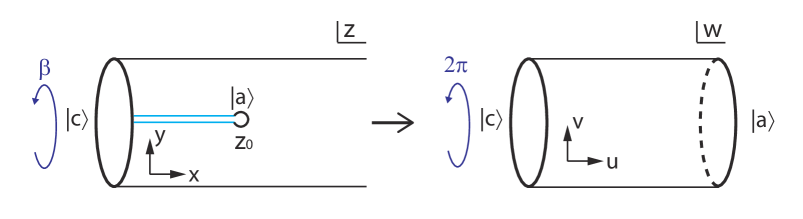
Figure 13: Euclidean spacetime for $\rho_{A}$ at finite temperature $\beta$, with $A=[0,L]$.

As a short summary, in the case $|b\rangle=|c\rangle$, the reduced density matrix $\rho_{A}(t\to\infty)$ is exactly the same as that at a finite temperature $\beta$. But for $|b\rangle\neq|c\rangle$, because the left boundary condition of the annulus is composed of both $|b\rangle$ and $|c\rangle$ segments, the limit $\rho_{A}(t\to\infty)$ of the reduced density matrix does not match exactly the thermal density matrix with external boundary condition $|c\rangle$ (recall that $|c\rangle$ describes the boundary condition at the physical boundary $x=0$). The latter density matrix is illustrated in Fig.13. - I.e., in general, the limit $\rho_{A}(t\to\infty)$ of the reduced density matrix still retains memory of the initial state $|b\rangle$ (compare Fig. 9).

6 Concluding remarks

In this work, we study the time evolution of the entanglement hamiltonian and related quantities for a finite interval of length $L$ at the end of a semi-infinite system after a global quantum quench into a (1+1) dimensional CFT from a special class of initial states, which are chosen to be the same conformal boundary states as those describing the physical boundary at the end $x=0$ of semi-infinite space. The results can be briefly summarized as follows.

– For times $t<L$, when the subsystem is not thermalized, the entanglement hamiltonian depends on both the hamiltonian density and the momentum density. After time $t=L$, when the subsystem $A$ is thermalized, the entanglement hamiltonian only depends on the hamiltonian density. In the long time limit $t\to\infty$, the entanglement hamiltonian (and therefore the reduced density matrix) for subsystem $A$ is exactly the same as that in a thermal ensemble at finite temperature $\beta^{-1}$.

– Using conformal mappings and the knowledge of boundary CFT, one can obtain both the entanglement entropy and the entanglement spectrum at arbitrary time $t$. In particular, for $t>L$, it is found that the spacing of entanglement spectrum approaches its long-time saturation value, i.e. that of the entanglement spectrum in a thermal ensemble at temperature $\beta^{-1}$, exponentially in time.

– The modular flows in the causal wedge of subsystem $A$ in Minkowski spacetime are studied. These flows provide us with very rich information on how the subsystem is thermalized. For $t<L$, these flows show a mixed feature of a thermal ensemble and a global quantum quench without thermalization. As time evolves, the feature of a thermal ensemble dominates gradually. For $t>L$, the distribution of the modular flows is independent of time, and looks the same as that of a thermal ensemble at finite temperature $\beta^{-1}$. In addition, we find a quantitative correspondence between these flows and the corresponding entanglement hamiltonians, as shown in Eq. (36). There are also interesting features of the modular flows corresponding to subsystem $B=(L,\infty)$, where thermalization never occurs, which we discuss.

– We also studied the case where the conformal boundary state describing the initial state is different from that describing the physical boundary at the end $x=0$ of semi-infinite space. It is found that even in the limit $t\to\infty$, the reduced density matrix $\rho_{A}$ is not exactly the same as that in a thermal state. This is as expected for a rational CFT which is integrable and where the full set of conformal boundary states is well characterized. Curious readers may ask what happens for an irrational CFT with a large central charge $c$. In the later case, however, it appears that we do not control the set of conformal boundary states (which should be composed of an infinite number of Ishibashi states in irrational CFTs with a discrete set of primaries) and of corresponding boundary condition changing operators. We note that our method could presumably be extended to irrational CFTs with a discrete spectrum of primaries, once the corresponding properties of the conformal boundary states and boundary condition changing operators are suitably well understood.

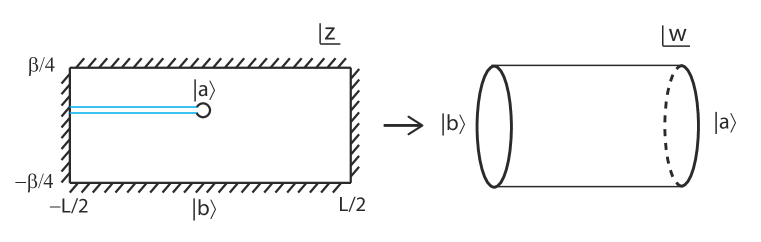
Figure 11: Setup for a subsystem $A=[-L/2,R]$ in a finite system $[-L/2,L/2]$ after a global quantum quench. The height of the rectangle is $\beta/2$. A small disc is removed at the entangling point as regularization, and the solid blue lines are branch cuts. The topology of a rectangle with a small disc removed is equivalent to an annulus. Therefore, one can use a conformal mapping $w=f(z)$ to map the rectangle in the $z$-plane to an annulus in the $w$-plane.

There are some future problems to study in detail:

– It would be interesting to study the time evolution of the entanglement hamiltonian and the corresponding modular flows for an interval in a finite system after a global quantum quench. It is known that quantum revival may be observed for a rational CFT due to the compact nature of the system [39]. It is expected that revival of the entanglement hamiltonian and of the modular flows should also be observed here. The setup for studying a finite system after a global quantum quench is shown in Fig.  11, where we have a rectangle in the $z$-plane with $z=x+iy$, $x\in[-L/2,L/2]$ and $y\in[-\beta/4,\beta/4]$. For simplicity, one can impose again (analogous to what was done in the main text of the present paper) the same conformal boundary condition along the horizontal boundary $x=\pm L/2$ as on the vertical boundary $y=\pm\beta/4$. Then, upon choosing the subregion $A$ to be a finite interval at the end of the finite position space $[-L/2,+L/2]$, the topology of this rectangle with a small disc removed at the entangling point is topologically equivalent to an annulus, as shown in Fig.  11. We can map the rectangle in the $z$-plane to an annulus in the $w$-plane based on a two-step conformal mapping: One can first map the rectangle in the complex $z$-plane to the right half complex plane (RHP) $\xi$-plane by using the Schwarz-Christoffel transformation (see e.g. Ref. [40]). Then the RHP with a small disc at $\xi_{0}$ removed can be mapped to an annulus in the $w$-plane by using the second formula in Eq. (11).

– It would be interesting to also study the case of inhomogeneous quantum quenches. In the current work, since the global quantum quench evolves from an initial state that is translation invariant, the density of modular flows is homogeneous and proportional to $\beta^{-1}$. For certain inhomogeneous quantum quenches, the inverse temperature is a function $\beta(x)$ of spatial position $x$, which indicates that the correlation length of the initial state is position-dependent. It is expected that one can observe modular flows with inhomogeneous density. Note that in Ref. [29], some general results and features of the evolution of the entanglement hamiltonian in inhomogeneous quenches have been studied, though it is still interesting to study certain concrete setups of inhomogeneous quantum quenches. See, e.g., the setups proposed in Refs. [43]. In particular, inhomogeneous hamiltonians are introduced in some setups, which are beyond the cases studied in [27]. (We note that the entanglement hamiltonian for certain inhomogeneous (1+1)d CFTs in the ground state has been studied most recently [44].)

7 Acknowledgements

We are grateful to the KITP Program “Quantum Physics of Information” (Sep 18 - Dec 15, 2017). This work was supported by the Gordon and Betty Moore Foundation’s EPiQS initiative through Grant No. GBMF4303 at MIT (XW), the NSF under Grants No. NSF PHY-1125915 (SR), and the NSF under Grant No. DMR-1309667 (AWWL).

Appendices

Appendix A On conformal mappings, etc

A.1 On entanglement hamiltonians

Entanglement hamiltonians for subsystem $A$ at the end of a semi-infinite system

For Eq. (13), first let us check the region $\beta\ll t<L$. By considering the limit $t,L\gg\beta$ and ignoring the contribution near $L-x\sim O(\beta)$, one can make the approximation $\sinh\left[\frac{\pi}{\beta}(x-L)\right]\simeq-\frac{1}{2}e^{\frac{\pi}{\beta}(L-x)}$. Then Eq. (13) can be approximated as

$$\begin{split}K_{A}(t<L)\simeq&\frac{\beta}{\pi}\int_{0}^{L}\frac{1}{2}\cdot\frac{e^{\frac{\pi}{\beta}(L-x)}\times\cosh\left[\frac{\pi}{\beta}(x-2t+L)\right]}{\cosh\left[\frac{2\pi}{\beta}(x-t)\right]}T(x-t)dx\\ &+\frac{\beta}{\pi}\int_{0}^{L}\frac{1+e^{-\frac{2\pi}{\beta}(x+2t-L)}}{2}\overline{T}(x+t)dx.\\ \end{split}$$ (49)

One finds that the result depends on whether $t<L/2$ or $L/2<t<L$ as follows. For $t<L/2$, one has

$$K_{A}\left(t<L/2\right)\simeq\frac{\beta}{2\pi}\int_{L-2t}^{L}\overline{T}(x+t)dx.$$ (50)

For ${L}/{2}<t<L$, one can check that

$$\begin{split}K_{A}\left(L/2<t<L\right)\simeq&\frac{\beta}{2\pi}\int_{0}^{2t-L}T(x-t)dx+\frac{\beta}{2\pi}\int_{0}^{L}\overline{T}(x+t)dx\\ =&\frac{\beta}{2\pi}\int_{0}^{2t-L}T_{00}(x,t)dx+\frac{\beta}{2\pi}\int_{2t-L}^{L}\overline{T}(x+t)dx.\end{split}$$ (51)

Now let us check the $t>L$ case. Again, by ignoring the contribution near $L-x\sim O(\beta)$, so that $\sinh\left[\frac{\pi}{\beta}(x-L)\right]\simeq-\frac{1}{2}e^{\frac{\pi}{\beta}(L-x)}$, and considering the limit $t,L\gg\beta$, $K_{A}(t)$ can be approximated as

$$\begin{split}K_{A}(t>L)\simeq&\frac{\beta}{\pi}\int_{L}^{0}\frac{1}{2}\cdot\frac{-e^{\frac{\pi}{\beta}(L-x)}\times e^{\frac{\pi}{\beta}(2t-x-L)}\times e^{\frac{\pi}{\beta}(x+L)}\times e^{\frac{\pi}{\beta}(2t+L-x)}}{e^{\frac{2\pi}{\beta}t}\times e^{\frac{2\pi}{\beta}L}\times e^{\frac{2\pi}{\beta}(t-x)}}T(x-t)dx\\ &+\frac{\beta}{\pi}\int_{L}^{0}\frac{1}{2}\cdot\frac{-e^{\frac{\pi}{\beta}(L-x)}\times e^{\frac{\pi}{\beta}(x+2t+L)}\times e^{\frac{\pi}{\beta}(x+L)}\times e^{\frac{\pi}{\beta}(x+2t-L)}}{e^{\frac{2\pi}{\beta}t}\times e^{\frac{2\pi}{\beta}L}\times e^{\frac{2\pi}{\beta}(x+t)}}\overline{T}(x+t)dx\\ =&\frac{\beta}{2\pi}\int_{0}^{L}\left[T(x-t)+\overline{T}(x+t)\right]dx\\ =&\frac{\beta}{2\pi}\int_{0}^{L}T_{00}(x,t)dx.\end{split}$$ (52)

In other words, $K_{A}(t)$ is proportional to the physical hamiltonian $H_{A}=\int_{0}^{L}T_{00}(x,t)dx$.

A.2 On modular flows in Minkowski spacetime

In this part, we give details of the behavior of the constant-$u$ flows in Fig.  7 and Fig.  8.

Vertical flows in region $|\,|$ in Fig.  7

Let us check the case $t_{0}<L$ first. Then region $|\,|$ in Fig.  7 is defined by the first formula in Eq. (32), based on which one can obtain

$$L+t_{0}>t+x>t-x>L-t_{0}>0.$$ (53)

By also considering $t_{0}<L$, one finds

$$|t-t_{0}|<L-x,\quad 0<L+x<t+t_{0}.$$ (54)

Then Eq. (34) can be approximated as

$$\frac{e^{\frac{2\pi}{\beta}(L-x)}}{e^{\frac{2\pi}{\beta}(L+x)}}\cdot\frac{e^{\frac{2\pi}{\beta}(t+t_{0})}}{e^{\frac{2\pi}{\beta}(t+t_{0})}}=e^{-2u}\quad\Rightarrow\quad x=\frac{\beta}{2\pi}u.$$ (55)

Now let us consider the case $t_{0}>L$. Then region $|\,|$ occupies the whole wedge, which is defined by

$$|t-t_{0}|<L-x<L+x,\quad x>0.$$ (56)

In addition, by considering $t_{0}>L$, one can obtain $t+t_{0}>L+x$. Then Eq. (34) can be approximated as

$$\frac{e^{\frac{2\pi}{\beta}(L-x)}}{e^{\frac{2\pi}{\beta}(L+x)}}\cdot\frac{e^{\frac{2\pi}{\beta}(t+t_{0})}}{e^{\frac{2\pi}{\beta}(t+t_{0})}}=e^{-2u}\quad\Rightarrow\quad x=\frac{\beta}{2\pi}u.$$ (57)

Left tilted flows in region $\backslash\backslash$ in Fig.  7

As shown in Fig.  7, the region $\backslash\backslash$ filled with left-tilted flows is defined by the second formula in Eq. (32), based on which one can find

$$|t-t_{0}|<L-x<t+t_{0}<L+x.$$ (58)

Then Eq. (34) can be approximated as

$$\frac{e^{\frac{2\pi}{\beta}(L-x)}}{e^{\frac{2\pi}{\beta}(L+x)}}\cdot\frac{e^{\frac{2\pi}{\beta}(L+x)}}{e^{\frac{2\pi}{\beta}(t+t_{0})}}=e^{-2u}\quad\Rightarrow\quad x-L+(t+t_{0})=\frac{\beta}{\pi}u.$$ (59)

Right tilted flows in region $//$ in Fig.  8

Let us check the case $t_{0}<L$ first. The region $//$ is defined in Eq. (37), based on which we find $|t-t_{0}|<x-L<t+t_{0}<x+L$. Then Eq. (34) can be simplified as

$$e^{\frac{2\pi}{\beta}(x-L-t-t_{0})}=e^{-2u}\quad\Rightarrow\quad x-L-(t+t_{0})=-\frac{\beta}{\pi}u.$$ (60)

Now let us consider the case $t_{0}>L$. Region $//$ is defined in Eq. (38), based on which we still have $|t-t_{0}|<x-L<t+t_{0}<x+L$. Then, again, Eq. (34) can be simplified as

$$\quad x-L-(t+t_{0})=-\frac{\beta}{\pi}u.$$ (61)

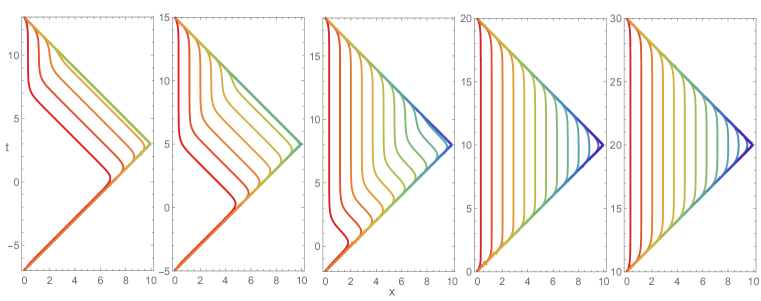
Figure 12: Constant-$u$ flows in the causal wedge of subsystem $A=\{(x,t_{0}),0\leq x\leq L\}$ at the end of a semi-infinite system in Minkowski spacetime. The parameters we use are $\beta=3.0$, and $L=10$. The observation times are chosen as $t_{0}=3,5,8,10,20$ from left to right.

A.3 Effect of $\beta$ on modular flows for a finite system after a global quench

Eqs. (35) and (39) that describe the flows in Fig.  7 and Fig.  8 are obtained in the limit $L\pm x,|t-t_{0}|\gg\beta$. It is natural to ask what happens if we increase $\beta$ in the initial state $e^{-(\beta/4)H_{\rm{CFT}}}|b\rangle$? Here we take the case in Fig.  7 for example. As we increase $\beta$, one finds that the constant-$u$ flows near the boundaries of regions $|\,|$ and $\backslash\backslash$ are no longer well approximated by straight lines, as shown in Fig.  12. In fact, as we further increase $\beta$, so that $\beta\geq L$, there will be no straight lines in the causal wedge. This can be easily understood by considering the limit $\beta\to\infty$, which corresponds to a CFT in its ground state, and there is essentially no quantum quench.

Appendix B Modular flows in Minkowski spacetime for a thermal ensemble, etc

B.1 Interval at the end of a semi-infinite system at finite temperature

For a finite interval $A=[0,L]$ at the end of a semi-infinite system at finite temperature $\beta^{-1}$, we have a semi-infinite annulus of circumference $\beta$ in the imaginary time $\text{Im}(z)$ direction. Again, we remove a small disc around the entangling point $L+i\tau$, where we can simply choose $\tau=0$. In addition, we impose boundary conditions described by conformal boundary states $|a\rangle$ and $|c\rangle$ at the small disc and along the physical boundary $x=0$, respectively. Then, by using the following conformal mapping

$$w=f(z)=\log\frac{e^{\frac{2\pi z}{\beta}}-e^{-\frac{2\pi L}{\beta}}}{e^{\frac{2\pi z}{\beta}}-e^{\frac{2\pi L}{\beta}}},$$ (62)

we map the semi-infinite annulus to a finite annulus in the $w$-plane, with conformal boundary conditions $|a\rangle$ and $|c\rangle$ at the two edges of the annulus. The circumference of the annulus in $\text{Im}\,w$ direction is $2\pi$. The width of the annulus in the $w$-plane can be obtained by

$$W=f(L-\epsilon)-f(0)=\log\left(\frac{e^{\frac{2\pi}{\beta}(L-\epsilon)}-e^{-\frac{2\pi}{\beta}L}}{e^{\frac{2\pi}{\beta}(L-\epsilon)}-e^{\frac{2\pi}{\beta}L}}\cdot\frac{1-e^{\frac{2\pi}{\beta}L}}{1-e^{-\frac{2\pi}{\beta}L}}\right),$$ (63)

which can be rewritten as

$$W=\log\frac{\sinh[\pi(2L-\epsilon)/\beta]}{\sinh(\pi\epsilon/\beta)}.$$ (64)

In the limit $L\gg\beta\gg\epsilon$, $W$ can be further simplified as

$$W\simeq\frac{2\pi}{\beta}L+\log\frac{\beta}{2\pi\epsilon}.$$ (65)

Based on the definition in Eq. (10), the von Neumann entropy has the form (keeping only the leading term in $L$)

$$S_{A}\simeq\frac{\pi c}{3\beta}\cdot L.$$ (66)

In addition, it is straightforward to find the exact form of entanglement hamiltonian as follows

$$K_{A}=\frac{\beta}{\pi}\int_{0}^{L}\frac{\sinh[\pi(L-x)/\beta]\sinh[\pi(L+x)/\beta]}{\sinh(2\pi L/\beta)}T_{00}(x)dx,$$ (67)

which may be simplified as

$$K_{A}(\beta)\simeq\frac{\beta}{2\pi}\int_{0}^{L}T_{00}(x)dx,$$ (68)

by ignoring the contributions near the entangling points $|L\pm x|\sim O(\beta)$.

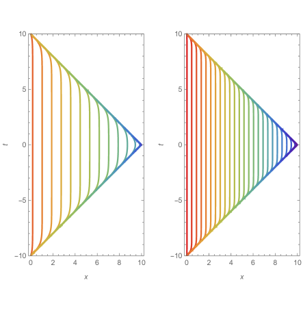
Figure 14: Constant-$u$ flows in the causal wedge of subsystem $A=\{(x,0),0\leq x\leq L\}$ at finite temperature $\beta^{-1}$ in Minkowski spacetime. The physical boundary is along $x=0$. The parameters we use are $L=10$, $\beta=3.0$ (left) and $\beta=1.5$ (right).

Now, we will study the constant-$u$ flows for subsystem $A$ in Minkowski spacetime. Based on the conformal mapping in Eq. (62), one can get

$$\frac{e^{\frac{4\pi}{\beta}x}-2e^{\frac{2\pi}{\beta}(x-L)}\cos\frac{2\pi}{\beta}y+e^{-\frac{2\pi}{\beta}2L}}{e^{\frac{4\pi}{\beta}x}-2e^{\frac{2\pi}{\beta}(x+L)}\cos\frac{2\pi}{\beta}y+e^{\frac{2\pi}{\beta}2L}}=e^{2u}.$$ (69)

Making the analytic continuation $y\to it$, one can further obtain the flows in Minkowski spacetime

$$\frac{e^{\frac{4\pi}{\beta}x}-2e^{\frac{2\pi}{\beta}(x-L)}\cosh\frac{2\pi}{\beta}t+e^{-\frac{2\pi}{\beta}2L}}{e^{\frac{4\pi}{\beta}x}-2e^{\frac{2\pi}{\beta}(x+L)}\cosh\frac{2\pi}{\beta}t+e^{\frac{2\pi}{\beta}2L}}=e^{2u}.$$ (70)

Shown in Fig.  14 are the constant-$u$ flows for different $\beta$, plotted according to Eq. (70). One can find that these constant-$u$ flows are equally distributed vertical lines. In addition, the density of these flows is proportional to $\beta^{-1}$. To understand these features, let us focus on the causal wedge of $A$ defined by

$$x\geq 0,\quad t>x-L,\quad t<-(x-L).$$ (71)

In the limit $L,x,t\gg\beta$, Eq. (70) can be simplified as

$$e^{\frac{4\pi}{\beta}(x-L)}=e^{2u},\quad\Rightarrow\quad x=\frac{\beta}{2\pi}u+L,$$ (72)

which describes the vertical flows in Fig.  14. In addition, one has $\Delta x=\frac{\beta}{2\pi}\Delta u$, and $1/\Delta x=\frac{2\pi}{\beta}\cdot\frac{1}{\Delta u}$, i.e., the density of these vertical lines is proportional to $\beta^{-1}$.

B.2 A semi-infinite interval $A$ in an infinite system after a global quench

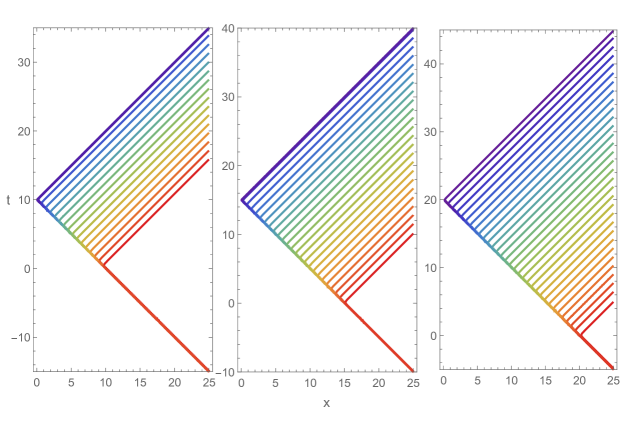
Figure 15: Constant-$u$ flows in the causal wedge of subsystem $A=\{(x,t_{0}),0\leq x\leq\infty\}$ in an infinite system after a global quantum quench. The parameters we use are $\beta=1.5$. The observation times are $t_{0}=10,15$ and $20$ from left to right.

The setup for a global quench in CFT can be described by the infinite strip given by $-\beta/4\leq\text{Im}(z)\leq\beta/4$ and $\text{Re}(z)\in\mathbb{R}$. We are interested in subsystem $A=(0,\infty)$, and therefore need to consider a cut $C=\{z=i\tau+x,x\geq 0\}$, where $|\tau|<\beta/4$. The conformal transformation is (as compared to Ref. [29], there is a sign difference here, introduced to simplify comparison with the conformal mapping used in the main text)

$$w=-\log\frac{\sinh\frac{\pi(z-i\tau)}{\beta}}{\cosh\frac{\pi(z+i\tau)}{\beta}},$$ (73)

based on which we can find the constant-$u$ flows in Euclidean spacetime

$$\frac{\sinh^{2}\frac{\pi x}{\beta}\cos^{2}\frac{\pi(y-\tau)}{\beta}+\cosh^{2}\frac{\pi x}{\beta}\sin^{2}\frac{\pi(y-\tau)}{\beta}}{\cosh^{2}\frac{\pi x}{\beta}\cos^{2}\frac{\pi(y+\tau)}{\beta}+\sinh^{2}\frac{\pi x}{\beta}\sin^{2}\frac{\pi(y+\tau)}{\beta}}=e^{-2u},$$ (74)

and (by taking $y\to it$ and $\tau\to it_{0}$)

$$\frac{\sinh^{2}\frac{\pi x}{\beta}\cosh^{2}\frac{\pi(t-t_{0})}{\beta}-\cosh^{2}\frac{\pi x}{\beta}\sinh^{2}\frac{\pi(t-t_{0})}{\beta}}{\cosh^{2}\frac{\pi x}{\beta}\cosh^{2}\frac{\pi(t+t_{0})}{\beta}-\sinh^{2}\frac{\pi x}{\beta}\sinh^{2}\frac{\pi(t+t_{0})}{\beta}}=e^{-2u}$$ (75)

in Minkowski spacetime. The constant-$u$ flows corresponding to subsystem $A$ are shown in Fig.15. As $t_{0}$ grows, the region $//$ filled with right-tilted lines grows all the way, due to the semi-infinite nature of both subsystems $A$ and $B$.

Equation (75) can be further simplified as

$$\frac{\cosh\frac{2\pi x}{\beta}-\cosh\frac{2\pi(t-t_{0})}{\beta}}{\cosh\frac{2\pi x}{\beta}+\cosh\frac{2\pi(t+t_{0})}{\beta}}=e^{-2u}.$$ (76)

Let us check the region $//$ filled with right-tilted lines, which is defined by

$$t-t_{0}<x,\quad t-t_{0}>-x,\quad t-t_{0}>x-2t_{0}.$$ (77)

In the limit $t\pm t_{0}\gg\beta$, then Eq. (76) can be approximated as

$$\frac{e^{\frac{2\pi x}{\beta}}}{e^{\frac{2\pi(t+t_{0})}{\beta}}}=e^{-2u}\quad\Rightarrow x-(t+t_{0})=-\frac{\beta}{\pi}u.$$ (78)

Similarly, if we study the flows for subsystem $B=(-\infty,0)$, one can observe a region $\backslash\backslash$ filled with left-tilted flows. This region is defined by

$$t-t_{0}>x,\quad t-t_{0}<-x,\quad t-t_{0}>-(x+2t_{0}).$$ (79)

In the limit $t\pm t_{0}\gg\beta$, Eq. (76) can be approximated as

$$\frac{e^{\frac{-2\pi x}{\beta}}}{e^{\frac{2\pi(t+t_{0})}{\beta}}}=e^{-2u}\quad\Rightarrow x+(t+t_{0})=\frac{\beta}{\pi}u.$$ (80)

References

References

- [1] D. N. Page, Phys. Rev. Lett. 71, 1291 (1993).
- [2] J. M. Deutsch, Phys. Rev. A 43, 2046 (1991).
- [3] R. V. Jensen, R. Shankar, Phys. Rev. Lett. 54, 1879–1882 (1985).
- [4] M. Srednicki, Phys. Rev. E 50, 888 (1994).
- [5] M. Rigol, V. Dunjko, M. Olshanii, Nature 452, 854 (2008).
- [6] J. Eisert, M. Friesdorf, C. Gogolin, Nat. Phys. 11, 124 (2015); arXiv:1408.5148.
- [7] A. M. Kaufman, et al., Science 353, 794 (2016).
- [8] M. Rigol, V. Dunjko, V. Yurovsky, and M. Olshanii, Phys. Rev. Lett. 98, 050405 (2007); arXiv:cond-mat/0604476.
-
[9]
See, e.g.,
M. A. Cazalilla,
Phys. Rev. Lett. 97, 156403 (2006); arXiv:cond-mat/0606236;
M. Cramer, C. M. Dawson, J. Eisert, and T. J. Osborne, Phys. Rev. Lett. 100, 030602 (2008); arXiv:cond-mat/0703314;
P. Calabrese, F. H. L. Essler, and M. Fagotti, Phys. Rev. Lett. 106, 227203 (2011); arXiv:1104.0154;
J. -S. Caux and R. M. Konik, Phys. Rev. Lett. 109, 175301 (2012); arXiv:1203.0901;
M. Fagotti and F. H. L. Essler, Phys. Rev. B 87, 245107 (2013); arXiv:1302.6944
J.-S. Caux and F. H. L. Essler, Phys. Rev. Lett. 110, 257203 (2013); arXiv:1301.3806
M. Kormos, M. Collura, and P. Calabrese, Phys. Rev. A 89, 013609 (2014); arXiv:1307.2142. - [10] S. Ryu and Y. Hatsugai, Phys. Rev. B 73, 245115 (2006); arXiv:cond-mat/0601237.
- [11] H. Li and F. D. M. Haldane, Phys. Rev. Lett. 101, 010504 (2008); arXiv:0805.0332.
- [12] F. Pollmann, E. Berg, A. M. Turner and Masaki Oshikawa, Phys. Rev. B 81, 064439 (2010); arXiv:0910.1811.
- [13] X.-L. Qi, H. Katsura, A. W. W. Ludwig, Phys. Rev. Lett. 108 (2012) 196402.
- [14] B. Bauer, L. Cincio, B. P. Keller, M. Dolfi, G. Vidal, S. Trebst, A. W. W. Ludwig, Nature Communications 5 (2014) 5137.
- [15] D. Blanco, H. Casini, L.-Y. Hung and R. Myers, JHEP 1308 (2013) 060; arXiv:1305.3182.
- [16] I. Peschel, J. Stat. Mech. P12005 (2004).
- [17] J. Bisognano and E. Wichmann, J. Math. Phys. 17, 303 (1976); J. Math. Phys. 16, 985 (1975).
- [18] W. Unruh, Phys. Rev. D 14, 870 (1976).
-
[19]
H. Casini, M. Huerta and R. Myers,
JHEP 1105 (2011) 036; arXiv:1102.0440;
P. D. Hislop and R. Longo, Commun. Math. Phys. 84, 71 (1982). - [20] G. Wong, I. Klich, L. Pando Zayas and D. Vaman, JHEP 1312 (2013) 020; arXiv:1305.3291.
- [21] H. Casini and M. Huerta, Class. Quant. Grav. 26, 185005 (2009); arXiv:0903.5284.
- [22] R. Longo, P. Martinetti and K. H. Rehren, Rev. Math. Phys. 22, 331 (2010); arXiv:0912.1106.
- [23] G. Wong, arXiv:1805.10651.
-
[24]
I. Peschel, M. Kaulke, and O. Legeza, Ann. der Phys. 8, 153 (1999);
I. Peschel and V. Eisler, J. Phys. A: Math. Theor. 42, 504003 (2009); arXiv:0906.1663. -
[25]
V. Eisler, I. Peschel,
J. Phys. A: Math. Theor. 50 284003 (2017);
arXiv:1703.08126;
V. Eisler, I. Peschel, arXiv:1805.00078; - [26] F. P. Toldin, F. F. Assaad, arXiv:1804.03163.
- [27] W. Zhu, Z. Huang, Y. -C. He, arXiv:1806.08060.
- [28] G. Giudici, T. Mendes-Santos, P. Calabrese, M. Dalmonte, arXiv:1807.01322.
- [29] J. Cardy and E. Tonni, J. Stat. Mech. 123103 (2016); arXiv:1608.01283.
- [30] C. T. Asplund, A. Bernamonti, F. Galli, T. Hartman, JHEP09 (2015) 110; arXiv:1506.03772
- [31] P. Calabrese and J. Cardy, J. Stat. Mech. P04010 (2005); arXiv:cond-mat/0503393.
- [32] P. Calabrese, J. Cardy, J. Stat. Mech. (2016) 064003; arXiv:1603.08267.
-
[33]
P. Calabrese and J. Cardy,
Phys. Rev. Lett. 96 136801 (2006); arXiv:cond-mat/0601225
P. Calabrese and J. Cardy, J. Stat. Mech. 0706 P008 (2007); arXiv:0704.1880. - [34] J. Cardy, J. Stat. Mech. (2016) 023103; arXiv:1507.07266
- [35] G. Mandal, R. Sinha and N. Sorokhaibam, JHEP 08 (2015) 013; arXiv:1501.04580.
- [36] M, Miyaji, S. Ryu, T. Takayanagi and X. Wen, JHEP 05 (2015) 152; arXiv:1412.6226.
- [37] J. Cardy, J. Stat. Mech. 023103 (2016); arXiv:1507.07266.
- [38] I. Affleck and A. Ludwig, Phys. Rev. Lett. 67 (1991) 161.
- [39] J. Cardy, Phys. Rev. Lett. 112, 220401 (2014); arXiv:1403.3040.
-
[40]
K. Kuns and D. Marolf,
JHEP 09 (2014) 082; arXiv:1406.4926;
G. Mandal, R. Sinha, T. Ugajin, arXiv:1604.07830. - [41] H. J. Borchers and J. Yngvason Journal of Mathematical Physics 40, 601 (1999).
- [42] John L.Cardy Nucl. Phys. B324 (1989) 581.
-
[43]
See, e.g.,
S. Sotiriadis and J. Cardy, J. Stat. Mech P11003 (2008); arXiv:0808.0116
D. Bernard and B. Doyon J. Phys. A 45 362001 (2012); arXiv:1202.0239
J. Viti, J.-M. Stephan, J. Dubail and M. Haque, EPL 115 (2016) 40011; arXiv:1507.08132;
J. Dubail, J. Stephan, J. Viti and P. Calabrese, SciPost Phys. 2, 002 (2017); arXiv:1606.04401;
K. Agarwal, E. G. D. Torre, J. Schmiedmayer and E. Demler, Phys. Rev. B 95, 195157 (2017); arXiv:1609.04046;
G. Ramírez, J. Rodríguez-Laguna, and G. Sierra, J. Stat. Mech. (2015) P06002; arXiv:1503.02695.
J. Rodríguez-Laguna, J. Dubail, G. Ramírez, P. Calabrese, and G. Sierra, J. Phys. A: Math. Theor. 50 164001 (2017); arXiv:1611.08559.
J. Dubail, J.-M, Stephan, and P. Calabrese, SciPost Phys. 3, 019 (2017); arXiv:1705.00679;
V. Eisler, D. Bauernfeind, Phys. Rev. B 96, 174301 (2017); arXiv:1708.05187;
X. Wen, Y. Wang, and S. Ryu, J. Phys. A: Math. Theor. 51 195004 (2018); arXiv:1711.02126;
X. Wen, J. -Q. Wu, Phys. Rev. B 97, 184309 (2018); arXiv:1802.07765. - [44] E. Tonni, J. Rodriguez-Laguna, and G. Sierra, J. Phys. A: Math. Theor. 4 043105 (2018); arXiv:1712.03557.