Will it Blend?
Composing Value Functions in Reinforcement Learning

Abstract

An important property for lifelong-learning agents is the ability to combine existing skills to solve unseen tasks. In general, however, it is unclear how to compose skills in a principled way. We provide a “recipe” for optimal value function composition in entropy-regularised reinforcement learning (RL) and then extend this to the standard RL setting. Composition is demonstrated in a video game environment, where an agent with an existing library of policies is able to solve new tasks without the need for further learning.

1 Introduction

A major challenge in artificial intelligence is creating agents capable of leveraging existing knowledge for inductive transfer. Lifelong learning, in particular, requires that an agent be able to act effectively when presented with a new, unseen task. A promising approach is to combine behaviours learned in various separate tasks to create new skills (Taylor & Stone, 2009). This compositional approach allows us to build rich behaviours from relatively simple ones, resulting in a (good!) combinatorial explosion in the agent’s abilities (Saxe et al., 2017). However, in general, it is unclear how to produce new optimal skills from known ones.

One approach to compositionality is Linearly-solvable Markov Decision Processes (LMDPs) (Todorov, 2007), which structure the reward function to ensure that the Bellman equation becomes linear in the exponentiated value function. Todorov (2009) proves that the optimal value functions of a set of LMDPs can be composed to produce the optimal value function for a composite task. This is a particularly attractive property, since solving new tasks requires no further learning. However, the LMDP framework has so far been restricted to the tabular case with known dynamics, limiting its usefulness.

Related work has focused on entropy-regularised reinforcement learning (RL) (Schulman et al., 2017; Haarnoja et al., 2017; Nachum et al., 2017), where rewards are augmented with an entropy-based penalty term. This has been shown to lead to improved exploration and rich, multimodal value functions.

Prior work (Haarnoja et al., 2018) has demonstrated that these value functions can be composed to approximately solve the intersection of tasks. We complement these results by proving optimal composition for the union of tasks in the total-reward, absorbing-state setting. Thus, any task lying in the “span” of a set of basis tasks can be solved immediately, without any further learning. We provide a “recipe” for optimally composing value functions, and demonstrate our method in a video game. Results show that an agent is able to compose existing policies learned from pixel input to generate new, optimal behaviours.

2 Background

A Markov decision process (MDP) is defined by the $4$-tuple $(\mathcal{S},\mathcal{A},\rho,r)$ where (i) the state space $\mathcal{S}$ is standard Borel; (ii) the action space $\mathcal{A}$ is finite (and therefore a compact metric space when equipped with the discrete metric); (iii) the transition dynamics $\rho$ define a Markov kernel $(s,a)\mapsto\rho_{(s,a)}$ from $\mathcal{S}\times\mathcal{A}$ to $\mathcal{S}$; and (iv) the reward $r$ is a real-valued function on $\mathcal{S}\times\mathcal{A}$ that is bounded and measurable.

In RL, an agent’s goal is to maximise its utility by making a sequence of decisions. At each time step, the agent receives an observation from $\mathcal{S}$ and executes an action from $\mathcal{A}$ according to its policy. As a consequence of its action, the agent receives feedback (reward) and transitions to a new state. Whereas the rewards represent only the immediate outcome, the utility captures the long-term consequences of actions. Historically, many utility functions have been investigated (Puterman, 2014), but in this paper we only consider the total-reward criterion (see Section 2.1).

We consider the class of MDPs with an absorbing set $\mathcal{G}$, which is a Borel subset of the state space. We augment the state space with a virtual state $g$ such that $\rho_{(s,a)}(\{g\})=1$ for all $(a,s)$ in $\mathcal{G}\times\mathcal{A}$, and $r=0$ after reaching $g$. In the control literature, this class of MDPs is often called stochastic shortest path problems (Bertsekas & Tsitsiklis, 1991), and naturally model domains that terminate after the agent achieves some goal.

We restrict our attention to stationary Markov policies, or simply policies. A policy $s\mapsto\pi_{s}$ is a Markov kernel from $\mathcal{S}$ to $\mathcal{A}$. Together with an initial distribution $\nu$ over $\mathcal{S}$, a policy defines a probability measure over trajectories. To formalise this, we construct the set of $n$-step histories inductively by defining $\mathcal{H}_{0}=\mathcal{S}$ and $\mathcal{H}_{n}=\mathcal{H}_{n-1}\times\mathcal{A}\times\mathcal{S}$ for $n$ in $\mathbb{N}$. The $n$-step histories represent the set of all possible trajectories of length $n$ in the MDP. The probability measure on $\mathcal{H}_{n}$ induced by the policy $\pi$ is then

$$P^{\pi}_{\nu,n}=\nu\otimes\underbrace{\pi\otimes\rho\otimes\cdots\otimes\pi\otimes\rho}_{n\text{ times}}.$$

Using the standard construction (Klenke, 1995), we can define a unique probability measure $P^{\pi}_{\nu}$ on $\mathcal{H}_{\infty}$ consistent with the measures $P^{\pi}_{\nu,n}$ in the sense that

$$P^{\pi}_{\nu}(\mathcal{E}\times\mathcal{A}\times\mathcal{S}\times\mathcal{A}\times\cdots)=P^{\pi}_{\nu,n}(\mathcal{E}),$$

for any $n$ in $\mathbb{N}$ and any Borel set $\mathcal{E}\subseteq\mathcal{H}_{n}$. If $\nu$ is concentrated on a single state $s$, we simply write $P^{\pi}_{\nu}=P^{\pi}_{s}$. Additionally for any real-valued bounded measurable function $f$ on $\mathcal{H}_{n}$, we define $\mathbb{E}^{\pi}_{\nu}[f]$ to be the expected value of $f$ under $P^{\pi}_{\nu}$.

Finally, we introduce the notion of a proper policy—a policy under which the probability of reaching $\mathcal{G}$ after $n$ steps converges to $1$ uniformly over $\mathcal{S}$ as $n\to\infty$. Our definition extends that of Bertsekas & Tsitsiklis (1995) to general state spaces, and is equivalent to the definition of transient policies used by James & Collins (2006):

Definition 1.

A stationary Markov policy $\pi$ is said to be proper if

$$\sup_{s\in\mathcal{S}}\sum_{t=0}^{\infty}P^{\pi}_{s}(s_{t}\not\in\mathcal{G})<\infty.$$

Otherwise, we say that $\pi$ is improper.

2.1 Entropy-Regularised RL

In the standard RL setting, the expected reward at state $s$ under policy $\pi$ is given by $\mathbb{E}_{a\sim\pi}\left[r(s,a)\right]$. Entropy-regularised RL (Ziebart, 2010; Fox et al., 2016; Haarnoja et al., 2017; Schulman et al., 2017; Nachum et al., 2017) augments the reward function with a term that penalises deviating from some reference policy $\bar{\pi}$. That is, the expected reward is given by $\mathbb{E}_{a\sim\pi}\left[r(s,a)\right]-\tau\text{KL}[\pi_{s}||\bar{\pi}_{s}]$, where $\tau$ is a positive scalar temperature parameter and $\text{KL}[\pi_{s}||\bar{\pi}_{s}]$ is the Kullback-Leibler divergence between $\pi$ and the reference policy $\bar{\pi}$ at state $s$. When $\bar{\pi}$ is the uniform random policy, the regularised reward is equivalent to the standard entropy bonus up to an additive constant (Schulman et al., 2017). This results in policies that are more robust to “winner’s curse” (Fox et al., 2016). Additionally, the reference policy can be used to encode prior knowledge through expert demonstration.

Based on the above regularisation, we define the $n$-step value function starting from $s$ and following policy $\pi$ as:

$$V_{\pi,n}(s)=\mathbb{E}^{\pi}_{s,n}\left[\sum^{n-1}_{t=0}r(s_{t},a_{t})-\tau\text{KL}[\pi_{s_{t}}||\bar{\pi}_{s_{t}}]\right].$$

Note that since the KL-divergence term is measurable (Dupuis & Ellis, 2011, Lemma 1.4.3), $V_{\pi,n}$ is well-defined. The infinite-horizon value function, which represents the total expected return after executing $\pi$ from $s$, is then

$$V_{\pi}(s)=\limsup_{n\to\infty}V_{\pi,n}(s).$$

Since the reward function and KL-divergence are bounded, $V_{\pi}$ is well defined. Similarly, we define the $Q$-function to be the expected reward after taking action $a$ in state $s$, and thereafter following policy $\pi$:

$$Q_{\pi}(s,a)=r(s,a)+\int_{\mathcal{S}}V_{\pi}(s^{\prime})\rho_{(a,s)}(ds^{\prime}).$$ (1)

Given the definitions above, we say that a measurable function $V^{*}$ is optimal if $V^{*}(s)=\sup_{\pi}V_{\pi}(s)$ for all $s$ in $\mathcal{S}$. Furthermore, a policy $\pi^{*}$ is optimal if $V_{\pi^{*}}=V^{*}$.

In the standard RL case, the optimal policy is always deterministic and is defined by $\operatorname*{argmax}_{a}Q^{*}(s,a)$. On the other hand, entropy-regularised problems may not admit an optimal deterministic policy. This results from the KL-divergence term, which penalises deviation from the reference policy $\bar{\pi}$. If $\bar{\pi}$ is stochastic, then a deterministic policy may incur more cost than a stochastic policy. To see this, consider the simple two-state MDP shown in Figure 1:

Figure 1: A two-state MDP with absorbing state $g$.

Given $\tau>0$ and a uniformly random reference policy, let $\pi$ be the deterministic policy that selects Right with probability $1$, and let $\pi_{\varepsilon}$ be the stochastic policy that selects Right with probability $1-\varepsilon$ and Left with probability $\varepsilon$. Then, choosing $\varepsilon$ small enough, we can guarantee that $V_{\pi_{\varepsilon}}>V_{\pi}$. Therefore for any $\tau>0$, the optimal policy is non-deterministic.

Proof.

First, the value of state $s$ under the policy $\pi$ is given by $V_{\pi}(s)=-1-\tau\log 2$. On the other hand, the expected number of steps from $s$ to $g$ under $\pi_{\varepsilon}$ is $1/(1-\varepsilon)$ so we have

$$V_{\pi_{\varepsilon}}(s)=-\frac{1+\varepsilon\log 2\varepsilon}{1-\varepsilon}-\log 2(1-\varepsilon).$$

Now, choose $\varepsilon$ such that

$$\varepsilon<\frac{\tau(\log 2-1/2)}{2+\tau}.$$ (2)

Then, from (2) we have that:

1. $\varepsilon<1/2$ and therefore $\log 2(1-\varepsilon)<0$,

2. $\log 2\varepsilon<2\varepsilon$, and

3. $\log 2-1/2<1$ and therefore $\varepsilon<\tau/(2+\tau)$

Using the above facts we get the chain of inequalities:

$$V_{\pi_{\varepsilon}}(s) \overset{\text{(i)}}{>}-\frac{1+\varepsilon\log(2\varepsilon)}{1-\varepsilon}\overset{\text{(ii)}}{>}-\frac{1+2\varepsilon}{1-\varepsilon}$$

$$\overset{\text{(iii)}}{>}-1-\tau/2-\varepsilon(2+\tau)$$

$$\overset{\text{(2)}}{>}-1-\tau\log 2.$$

The last inequality follows directly from (2), giving $V_{\pi_{\varepsilon}}(s)>V_{\pi}(s)$. ∎

3 Soft Value and Policy Iteration

In this section, we investigate the total-reward, entropy-regularised criterion defined above. While value and policy iteration in entropy-regularised RL have been analysed previously (Nachum et al., 2017), convergence results are limited to discounted MDPs. We sketch an argument that an optimal proper policy exists under the total-reward criterion and that the soft versions of value and policy iteration (see Algorithms 1 and 2) converge to optimal solutions.

We begin by defining the Bellman operators:

$$[\mathcal{T}_{\pi}V_{\pi}](s) =\int_{\mathcal{A}}Q_{\pi}(s,a)\pi_{s}(da)-\tau\text{KL}[\pi_{s}||\bar{\pi}_{s}],$$ (3)

$$[\mathcal{T}V](s) =\sup_{\pi}[\mathcal{T}_{\pi}V](s).$$ (4)

Equations (3) and (4) are analogous to the standard Bellman operator and Bellman optimality operator respectively. Note that since the optimal policy may not be deterministic, the Bellman optimality operator selects the supremum over policies instead of actions.

We also define the soft Bellman operator

$$[\mathcal{L}V_{\pi}](s)=\tau\log\int_{\mathcal{A}}\exp\left(Q_{\pi}(s,a)/\tau\right)\pi_{s}(da).$$ (5)

Here $\mathcal{L}$ is referred to as “soft”, since it is a smooth approximation of the $\max$ operator. The soft Bellman operator is connected to the Bellman optimality operator through the following result:

Lemma 1.

Let $V:\mathcal{S}\to\mathbb{R}$ be a bounded measurable function. Then $\mathcal{T}V=\mathcal{L}V$ and the supremum is attained uniquely by the Boltzmann policy $\mathcal{B}[V]$ defined by

$$\dfrac{d\mathcal{B}_{s}[V]}{d\bar{\pi}_{s}}(a)=\frac{\exp\big{(}Q(s,a)/\tau\big{)}}{\int_{A}\exp\big{(}Q(s,a^{\prime})/\tau\big{)}\bar{\pi}(da^{\prime}|s)}.$$

Proof.

Follows directly from Dupuis & Ellis (2011, Proposition 1.4.2). ∎

Analogous to the standard RL setting, we can define value and policy iteration in the entropy-regularised context, where the Bellman operators are replaced with their “soft” equivalents:

Algorithm 1 Soft Value Iteration

  Input: MDP, temperature $\tau>0$, bounded function $V$

  Output: Optimal value function $V^{*}$

  initialize $V^{*}\leftarrow V$

  repeat

     replace $V\leftarrow V^{*}$

     apply soft Bellman operator $V^{*}\leftarrow\mathcal{L}[V]$

  until convergence

Algorithm 2 Soft Policy Iteration

  Input: MDP, temperature $\tau>0$, proper policy $\pi$

  Output: Optimal policy $\pi^{*}$

  initialize $\pi^{*}\leftarrow\pi$

  repeat

     replace $\pi\leftarrow\pi^{*}$

     policy evaluation:

      find $V_{\pi}$, the fixed-point of $\mathcal{T}_{\pi}$

     policy improvement:

      compute the Boltzmann policy $\pi^{*}\leftarrow\mathcal{B}[V_{\pi}]$

  until convergence

Following closely along the lines of Bertsekas & Tsitsiklis (1991) and James & Collins (2006), but taking special care to account for the fact that optimal policies are not necessarily deterministic, it can be shown that the above algorithms converge to optimal solutions.

Theorem 1.

Suppose that Assumptions 1 and 2 (James & Collins, 2006) hold and that the optimal value function is bounded above. Then:

1. there exists an optimal proper policy;

2. the optimal value function is the unique bounded measurable solution to the optimality equation;

3. the soft policy iteration algorithm converges to the policy starting from any proper policy;

4. the soft value iteration algorithm converges to the optimal value function starting from any proper policy.

4 Compositionality

In lifelong learning, an agent is presented with a series of tasks drawn from some distribution. The goal is to exploit knowledge gained in previous tasks to improve performance in the current task. We consider an environment with fixed state space $\mathcal{S}$, action space $\mathcal{A}$, deterministic transition dynamics $\rho$, and absorbing set $\mathcal{G}$. Let $\mathcal{D}$ be a fixed but unknown distribution over $(\mathcal{S},\mathcal{A},\rho,r)$. The agent is then presented with tasks sampled from $\mathcal{D}$, which differ only in their reward functions. In this section, we describe a compositional approach for tackling this problem.

Suppose that the reward functions drawn from $\mathcal{D}$ differ only on the absorbing set $\mathcal{G}$. This restriction was introduced by Todorov (2009), and is a strict subset of the successor representations framework (Dayan, 1993; Barreto et al., 2017). Given a library of previously-solved tasks, we can combine their $Q$-functions to solve any task lying in the “span” of the library without further learning:

Theorem 2 (Optimal Composition).

Let $\mathcal{M}_{1},\ldots,\mathcal{M}_{n}$ be a library of tasks drawn from $\mathcal{D}$. Let $Q^{*,k}_{\tau}$ be the optimal entropy-regularised $Q$-function, and $r_{k}$ be the reward function for $\mathcal{M}_{k}$. Define the vectors

$$\mathbf{r}=[r_{1},\ldots,r_{n}]\quad\text{ and }\quad\mathbf{Q}^{*}_{\tau}=[Q^{*,1}_{\tau},\ldots,Q^{*,n}_{\tau}].$$

Given a set of non-negative weights $\mathbf{w}$, with $||\mathbf{w}||_{1}=1$, consider a further task drawn from $\mathcal{D}$ with reward function satisfying $r=\tau\log\left(||\exp(\mathbf{r}/\tau)||_{\mathbf{w}}\right)$ for all $s$ in $\mathcal{G}$, where $||\cdot||_{\mathbf{w}}$ denotes the weighted $1$-norm. Then the optimal $Q$-value for this task is given by:

$$Q^{*}_{\tau}=\tau\log\left(||\exp(\mathbf{Q}^{*}_{\tau}/\tau)||_{\mathbf{w}}\right).$$ (6)

That is, the optimal $Q$-functions for the library of tasks can be composed to form $Q^{*}_{\tau}$.

Proof.

Since $\rho$ is deterministic, we can find a measurable function $f:\mathcal{S}\times\mathcal{A}\to\mathcal{S}$ such that $\rho_{(s,a)}=\delta_{f(s,a)}$. For any $Q$-function, define the desirability function

$$Z(s,a)=\exp\left(Q(s,a)/\tau\right),$$

and define the operator $\mathcal{U}$ on the space of non-negative bounded measurable functions by

$$[\mathcal{U}Z](s,a)=\exp\left(r(s,a)/\tau\right)\int_{\mathcal{A}}Z(f(s,a),a)\bar{\pi}_{s}(da^{\prime}).$$

We now show that the desirability function of $Q_{\tau}^{*}$ is a fixed point of $\mathcal{U}$. Since $V_{\tau}^{*}$ is the fixed point of the Bellman optimality operator, by combining Equation (1), Lemma 1 and Theorem 1, we have

$$V_{\tau}^{*}(s)=\tau\log\int_{\mathcal{A}}\exp\left(Q^{*}_{\tau}(f(s,a),a^{\prime})/\tau\right)\bar{\pi}_{s}(da^{\prime})$$

$$\text{and }Q^{*}_{\tau}(s,a)=r(s,a)+V^{*}_{\tau}(f(s,a)).$$

Then it follows that

$$[\mathcal{U}Z^{*}_{\tau}](s,a) =e^{r(s,a)/\tau}\int\exp\left(Q^{*}_{\tau}/\tau\right)d(\rho_{(s,a)}\otimes\bar{\pi}_{s})$$

$$=e^{r(s,a)/\tau}\exp\left(V^{*}_{\tau}(f(s,a))/\tau\right)=Z^{*}_{\tau}(s,a).$$

Hence $Z^{*}_{\tau}$ is a fixed point of $\mathcal{U}$. Under the assumptions on the reward function $r$, the optimal $Q$-value satisfies $Q^{*}_{\tau}=\tau\log\left(||\exp(\mathbf{Q}^{*}_{\tau}/\tau)||_{\mathbf{w}}\right)$ on $\mathcal{G}$. Therefore, restricted to $\mathcal{G}$, $Z^{*}_{\tau}$ is a linear combination of the desirability functions for the family of tasks. Since (6) holds on $\mathcal{G}$ and it is clear that $\mathcal{U}$ is a linear operator, then (6) holds everywhere. ∎

The following lemma links the previous result to the standard RL setting. Recall that entropy-regularisation appends a temperature-controlled penalty term to the reward function. As the temperature parameter tends to $0$, the reward provided by the environment dominates the entropy penalty, and the problem reduces to the standard RL case:

Lemma 2.

Let $\{\tau_{n}\}^{\infty}_{n=1}$ be a sequence in $\mathbb{R}$ such that $\tau_{n}\downarrow 0$. Let $Q^{*}_{\tau_{n}}$ be the optimal $Q$-value function for $\text{MDP}(\tau_{n})$: the entropy-regularised MDP with temperature parameter $\tau_{n}$. Let $Q^{*}_{0}$ be the optimal $Q$-value for the standard MDP. Then $Q^{*}_{\tau_{n}}\uparrow Q^{*}_{0}$ as $n\to\infty$.

Proof.

First note that for a fixed policy $\pi$, state $s$ and action $a$, we have $Q_{\tau_{n}}^{\pi}(s,a)\uparrow Q_{0}^{\pi}(s,a)$ as $n\to\infty$. This follows directly from the definition of the entropy-regularised value function, and the fact that the KL-divergence is non-negative. Then using Lemma 3.14 (Hinderer, 1970) to interchange the limit and supremum, we have

$$\lim_{n\to\infty}Q^{*}_{\tau_{n}} =\lim_{n\to\infty}\sup_{\pi}Q^{\pi}_{\tau_{n}}=\sup_{\pi}\lim_{n\to\infty}Q^{\pi}_{\tau_{n}}$$

$$=\sup_{\pi}Q_{0}^{\pi}=Q_{0}^{*}.$$

Since $Q_{\tau_{n}}^{\pi}\uparrow Q_{0}^{\pi}$, we have $Q^{*}_{\tau_{n}}\uparrow Q^{*}_{0}$ as $n\to\infty$. ∎

Finally, we show that composition holds in the standard RL setting by taking the low-temperature limit of Theorem 2.

Corollary 1.

Let $\{\tau_{n}\}^{\infty}_{n=1}$ be a sequence in $\mathbb{R}$ such that $\tau_{n}\downarrow 0$. Then $\max\mathbf{Q^{*}_{\tau_{n}}}\uparrow Q^{*}_{0}$ as $n\to\infty$.

Proof.

For a fixed state $s$ and action $a$ and a possible reordering of the vector $\mathbf{Q^{*}_{0}}(s,a)$, we may suppose, without loss of generality, that $Q^{*,1}_{0}(s,a)=\max\mathbf{Q^{*}_{0}}(s,a)$. Then by Lemma 2, we can find an $N$ in $\mathbb{N}$ such that

$$Q^{*,1}_{\tau_{n}}(s,a)=\max\mathbf{Q^{*}_{\tau_{n}}}(s,a)\text{ for all $n\geq N$}.$$

Since $\log$ is continuous, we have from Theorem 2 that

$$\lim_{n\to\infty}Q^{*}_{\tau_{n}} =\log\left(\lim_{n\to\infty}||\exp(\mathbf{Q^{*}_{\tau_{n}}})||_{\mathbf{w}}^{1/\tau_{n}}\right),$$

where $||\cdot||^{p}_{\mathbf{w}}$ denotes the weighted $p$-norm. By factoring $\exp(Q^{*,1}_{\tau_{n}})$ out of $||\exp(\mathbf{Q^{*}_{\tau_{n}}})||_{\mathbf{w}}^{1/\tau_{n}}$, we are left with

$$||1,\exp(\Delta_{2}),\ldots,\exp(\Delta_{k})||_{\mathbf{w}}^{1/\tau_{n}},$$

where $\Delta_{i}=Q^{*,i}_{\tau_{n}}-Q^{*,1}_{\tau_{n}}$ for $i=2,\ldots,k$. Since $Q^{*,1}_{\tau_{n}}(s,a)$ is the maximum of $\mathbf{Q^{*}_{\tau_{n}}}(s,a)$ for all $n\geq N$, the limit as $n\to\infty$ of the above is $1$. Then it follows that

$$\lim_{n\to\infty}Q^{*,1}_{\tau_{n}}(s,a) =\log\left(\lim_{n\to\infty}\exp(Q^{*,1}_{\tau_{n}}(s,a))\right)$$

$$=Q^{*,1}_{0}(s,a).$$

Since $s$ and $a$ were arbitrary and $Q^{*,m}_{\tau_{n}}\uparrow Q^{*,m}_{0}$, we have that $\max\mathbf{Q^{*}_{\tau_{n}}}\uparrow Q^{*}_{0}$ as $n\to\infty$. ∎

Comparing Theorem 2 to Corollary 1, we see that as the temperature parameter decreases to zero, the weight vector has less influence on the composed $Q$-function. In the limit, the optimal $Q$-function is independent of the weights and is simply the maximum of the library functions. This suggests a natural trade-off between our ability to interpolate between $Q$-functions, and the stochasticity of the optimal policy. Furthermore, Corollary 1 mirrors that of generalised policy improvement (Barreto et al., 2017), which shows that computing the maximum of a set of $Q$-functions results in an improved $Q$-function. In our case, the resulting $Q$-function is not merely an improvement, but is in fact optimal.

The composition described in this section can be viewed as an –OR– task composition: if objectives of two tasks are to achieve goals $A$ and $B$ respectively, then the composed $Q$-function will achieve $A$–OR–$B$ optimally. Haarnoja et al. (2018) show that an approximate –AND– composition is also possible for entropy-regularised RL. That is, if the goals $A$ and $B$ partially overlap, the composed $Q$-function will achieve $A$–AND–$B$ approximately. The idea is that the optimal $Q$-function for the composite task can be approximated by the average of the library $Q$-functions. We include their results for completeness:

Lemma 3 (Haarnoja et al., 2018).

Let $Q^{*,1}_{\tau}$ and $Q^{*,2}_{\tau}$ be the optimal $Q$-functions for two tasks drawn from $\mathcal{D}$ with rewards $r_{1}$ and $r_{2}$. Define the averaged $Q$-function $Q_{\text{ave}}:=(Q^{*,1}_{\tau}+Q^{*,2}_{\tau})/2$. Then the optimal $Q$-function $Q^{*}_{\tau}$ for the task with reward function $r=(r_{1}+r_{2})/2$ satisfies

$$Q_{\text{ave}}\geq Q^{*}_{\tau}\geq Q_{\text{ave}}-C^{*}_{\tau},$$

where $C^{*}_{\tau}$ is a fixed point of

$$\tau\mathbb{E}_{s^{\prime}\sim\rho(s,a)}\left[D_{\frac{1}{2}}\left(\pi_{s}^{*,1}||\pi_{s}^{*,2}\right)+\max_{a^{\prime}}C(s^{\prime},a^{\prime})\right],$$

the policy $\pi_{s}^{*,i}$ is the optimal Boltzmann policy for task $i$, and $D_{\frac{1}{2}}(\cdot||\cdot)$ is the Rényi divergence of order $\frac{1}{2}$.

Theorem 3 (Haarnoja et al., 2018).

Using the definitions in Lemma 3, the value of the composed policy $\pi^{\text{ave}}$ satisfies

$$Q_{\pi^{\text{ave}}}\geq Q^{*}_{\tau}-F^{*}_{\tau},$$

where $F^{*}_{\tau}$ is a fixed point of

$$\tau\mathbb{E}_{s^{\prime}\sim\rho(s,a)}\left[\mathbb{E}_{a^{\prime}\sim\pi^{\text{ave}}_{s^{\prime}}}\left[C^{*}_{\tau}(s^{\prime},a^{\prime})-F(s^{\prime},a^{\prime})\right]\right].$$

We believe that the low-temperature result from Lemma 2 can be used to obtain similar results for the standard RL framework. We provide empirical evidence of this in the next section, and leave a formal proof to future work.

5 Experiments

To demonstrate composition, we perform a series of experiments in a grid-world video game (Figure 2(b)). The goal of the game is to collect items of different colours and shapes. The agent has four actions that move it a single step in any of the cardinal directions, unless it collides with a wall.Each object in the domain is one of two shapes (squares and circles), and one of three colours (blue, beige and purple), for a total of six objects (see Figure 2(a)).

(a) Items to be collected.

(b) Layout of the grid-world.

Figure 2:

We construct a number of different tasks based on the objects that the agent must collect, the task’s name specifying the objects to be collected. For example, Purple refers to the task where an agent must collect any purple object, while BeigeSquare requires collecting the single beige square.

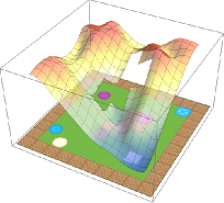
(a)

(b)

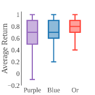
(c)

Figure 3: (3(a)) The optimal value function for PurpleOrBlue, which is produced by composing the Purple and Blue $Q$-functions. The multimodality of the composite value function is clearly visible. (3(b)) Sample trajectories for the composite PurpleOrBlue task, with the agent beginning at different positions. The agent selects the shortest path to any of the target objects. (3(c)) Returns from $50$k episodes. The first two box plots are the results of acting in the PurpleOrBlue task using only one of the base $Q$-functions, while the third uses the composite $Q$-function.

For each task, the episode begins by randomly positioning the six objects and the agent. At each timestep, the agent receives a reward of $-0.1$. If the correct object is collected, the agent receives a reward of $1$ and the episode terminates. We first learn to solve a number of base tasks using (soft) deep $Q$-learning (Mnih et al., 2015; Schulman et al., 2017), where each task is trained with a separate network. The resulting networks are collected into a library from which we will later compose new $Q$-functions.

The input to our network is a single RGB frame of size $84\times 84$, which is passed through three convolutional layers and two fully-connected layers before outputting the predicted Q-values for the given state. Using the results in Section 4, we compose optimal $Q$-functions from those in the library.

5.1 –OR– Composition

Here we consider new tasks that can be described as the union of a set of base tasks in the standard RL setting. We train an agent separately on the Purple and Blue tasks, adding the corresponding $Q$-functions to our library. We use Corollary 1 to produce the optimal $Q$-function for the composite PurpleOrBlue task, which requires the agent to pick up either blue or purple objects, without any further learning. Results are given in Figure 3.

The local maxima over blue and purple objects illustrates the multimodality of the value function (Figure 3(a)). This is similar to approaches such as soft $Q$-learning (Haarnoja et al., 2017), which are also able to learn multimodal policies. However, we have observed that directly learning a truly multimodal policy for the composite task can be difficult. If the entropy regularisation is too high, the resulting policy is extremely stochastic. Too low a temperature results in a loss of multimodality, owing to winner’s curse. It is instead far easier to learn unimodal value functions for each of the base tasks, and then compose them to produce optimal multimodal value functions.

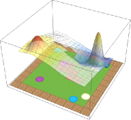
(a) BeigeSquare: $0.0$

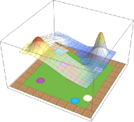
(b) BeigeSquare: $0.05$

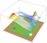
(c) BeigeSquare: $0.1$

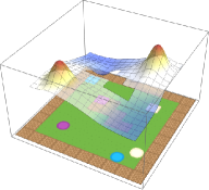
(d) BeigeSquare: $0.5$

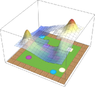
(e) BeigeSquare: $0.9$

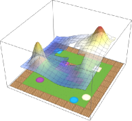
(f) BeigeSquare: $0.95$

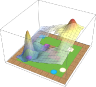
(g) BeigeSquare: $1.0$

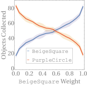
(h)

Figure 4: (4(a)–4(g)) Weighted composed value function for the task BeigeSquareOrPurpleCircle. The weight assigned to the $Q$-function for BeigeSquare is varied from $0$ to $1$. (4(h)) The number of beige squares compared to purple circles collected by the agent as the weights are varied in steps of $0.05$. Results for each weight were averaged over $80$ runs of $100$ episodes.

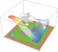
(a)

(b)

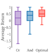
(c)

Figure 5: (5(a)) The approximately optimal value function of the composed policies. Local optima are clearly visible. (5(b)) Sample trajectories from the composed policy beginning from different starting positions. The agent exhibits suboptimal, but sensible behaviour near beige squares. (5(c)) The IQR of returns from $50$k episodes. The first box plot is the return from the optimal solution to the union of tasks, the second is the result of the approximate intersection of tasks, and the third is the true optimal policy.

5.2 Linear Task Combinations

In Theorem 2 we showed that in the entropy-regularised setting, the composed $Q$-function is dependent on a weight vector $\mathbf{w}$. This allows us to achieve a more general type of composition. In particular, we can immediately compute any optimal $Q$-function that lies in the “span” of the library $Q$-functions. Indeed, according to Theorem 2 the exponentiated optimal $Q$-function is a linear combination of the exponentiated library functions. Therefore, the weights can be used to modulate the relative importance of the library functions—modelling the situation in which an agent has multiple concurrent objectives of unequal importance.

We illustrate the effect of the weight vector $\mathbf{w}$ using soft $Q$-learning with a temperature parameter $\tau=1$. We construct a new task by composing the tasks PurpleCircle and BeigeSquare, and assign different weights to these tasks. The different weighted value functions are given in Figure 4.

5.3 –AND– Composition

Here we consider tasks which can be described as the intersection of tasks in the library. In general, this form of composition will not yield an optimal policy for the composite task owing to the presence of local optima in the composed value function. However, in many cases we can obtain a good approximation to the composite task by simply averaging the Q-values for the constituent tasks. While Haarnoja et al. (2018) considers this type of composition in the entropy-regularised case, we posit that this can be extended to the standard RL setting by taking the low-temperature limit. We illustrate this by composing the optimal policies for the Blue and Square tasks, which produces a good approximation to the optimal policy for collecting the blue square. Results are shown in Figure 5.

5.4 Temporal

Our final experiment demonstrates the use of composition to long-lived agents. We compose the base $Q$-functions for the tasks Blue, Beige and Purple, and use the resulting $Q$-function to solve the task of collecting all objects. Sample trajectories are illustrated by Figure 6.

Despite the fact that the individual tasks terminate after collecting the required object, if we allow the episode to continue, the composed $Q$-function is able to collect all objects in a greedy fashion. The above shows the power of composition—if we possess a library of skills learned from previous tasks, we can compose them to solve any task in their union continually.

(a)

(b)

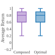
(c)

Figure 6: (6(a)) and (6(b)) Sample trajectories for the task of collecting all objects. (6(c)) Returns from $50$k episodes. The first box plot is the return of the composed $Q$-function, while the second is the result of DQN trained to collect all objects explicitly.

6 Conclusion

We showed that in entropy-regularised RL, value functions can be optimally composed to solve the union of tasks. Extending this result by taking the low-temperature limit, we showed that composition is also possible in standard RL. However, there is a trade-off between our ability to smoothly interpolate between tasks, and the stochasticity of the optimal policy. We demonstrated, in a high-dimensional environment, that a library of optimal $Q$-functions can be composed to solve composite tasks consisting of unions, intersections or temporal sequences of simpler tasks. The proposed compositional framework is a step towards lifelong-learning agents that are able to combine existing skills to solve new, unseen problems.

References

- Barreto et al. (2017) Barreto, A., Dabney, W., Munos, R., Hunt, J., Schaul, T., van Hasselt, H., and Silver, D. Successor features for transfer in reinforcement learning. In Advances in neural information processing systems, pp. 4055–4065, 2017.
- Bertsekas & Tsitsiklis (1991) Bertsekas, D.P. and Tsitsiklis, J.N. An analysis of stochastic shortest path problems. Mathematics of Operations Research, 16(3):580–595, 1991.
- Bertsekas & Tsitsiklis (1995) Bertsekas, D.P. and Tsitsiklis, J.N. Neuro-dynamic programming: an overview. In Proceedings of the 34th IEEE Conference on Decision and Control, volume 1, pp. 560–564. IEEE, 1995.
- Dayan (1993) Dayan, P. Improving generalization for temporal difference learning: The successor representation. Neural Computation, 5(4):613–624, 1993.
- Dupuis & Ellis (2011) Dupuis, P. and Ellis, R. A weak convergence approach to the theory of large deviations. 2011.
- Fox et al. (2016) Fox, R., Pakman, A., and Tishby, N. Taming the noise in reinforcement learning via soft updates. In 32nd Conference on Uncertainty in Artificial Intelligence, 2016.
- Haarnoja et al. (2017) Haarnoja, T., Tang, H., Abbeel, P., and Levine, S. Reinforcement learning with deep energy-based policies. In International Conference on Machine Learning, pp. 1352–1361, 2017.
- Haarnoja et al. (2018) Haarnoja, T., Pong, V., Zhou, A., Dalal, M., Abbeel, P., and Levine, S. Composable deep reinforcement learning for robotic manipulation. arXiv preprint arXiv:1803.06773, 2018.
- Hinderer (1970) Hinderer, K. Foundations of non-stationary dynamic programming with discrete time parameter. In Lecture Notes in Operations Research and Mathematical Systems, volume 33. 1970.
- James & Collins (2006) James, H.W. and Collins, E.J. An analysis of transient Markov decision processes. Journal of applied probability, 43(3):603–621, 2006.
- Klenke (1995) Klenke, A. Probability Theory: A Comprehensive Course, volume 158. 1995. ISBN 9781447153603.
- Mnih et al. (2015) Mnih, V., Kavukcuoglu, K., Silver, D., Rusu, A.A., Veness, J., Bellemare, M.G., Graves, A., Riedmiller, M., Fidjeland, A.K., Ostrovski, G., et al. Human-level control through deep reinforcement learning. Nature, 518(7540):529, 2015.
- Nachum et al. (2017) Nachum, O., Norouzi, M., Xu, K., and Schuurmans, D. Bridging the gap between value and policy based reinforcement learning. In Advances in Neural Information Processing Systems, pp. 2772–2782, 2017.
- Puterman (2014) Puterman, M.L. Markov decision processes: discrete stochastic dynamic programming. John Wiley & Sons, 2014.
- Saxe et al. (2017) Saxe, A.M., Earle, A.C., and Rosman, B.S. Hierarchy through composition with multitask LMDPs. Proceedings of the 34th International Conference on Machine Learning, 70:3017–3026, 2017.
- Schulman et al. (2017) Schulman, J., Abbeel, P., and Chen, X. Equivalence between policy gradients and soft Q-learning. pp. 1–15, 2017.
- Taylor & Stone (2009) Taylor, M.E. and Stone, P. Transfer learning for reinforcement learning domains: a survey. Journal of Machine Learning Research, 10:1633–1685, 2009.
- Todorov (2007) Todorov, E. Linearly-solvable Markov decision problems. In Advances in Neural Information Processing Systems, pp. 1369–1376, 2007.
- Todorov (2009) Todorov, E. Compositionality of optimal control laws. In Advances in Neural Information Processing Systems, pp. 1856–1864, 2009.
- Ziebart (2010) Ziebart, B.D. Modeling purposeful adaptive behavior with the principle of maximum causal entropy. Carnegie Mellon University, 2010.