Estimating Cellular Goals from
High-Dimensional Biological Data

Abstract.

Optimization-based models have been used to predict cellular behavior for over 25 years. The constraints in these models are derived from genome annotations, measured macro-molecular composition of cells, and by measuring the cell’s growth rate and metabolism in different conditions. The cellular goal (the optimization problem that the cell is trying to solve) can be challenging to derive experimentally for many organisms, including human or mammalian cells, which have complex metabolic capabilities and are not well understood. Existing approaches to learning goals from data include (a) estimating a linear objective function, or (b) estimating linear constraints that model complex biochemical reactions and constrain the cell’s operation. The latter approach is important because often the known/observed biochemical reactions are not enough to explain observations, and hence there is a need to extend automatically the model complexity by learning new chemical reactions. However, this leads to nonconvex optimization problems, and existing tools cannot scale to realistically large metabolic models. Hence, constraint estimation is still used sparingly despite its benefits for modeling cell metabolism, which is important for developing novel antimicrobials against pathogens, discovering cancer drug targets, and producing value-added chemicals. Here, we develop the first approach to estimating constraint reactions from data that can scale to realistically large metabolic models. Previous tools have been used on problems having less than 75 biochemical reactions and 60 metabolites, which limits real-life-size applications. We perform extensive experiments using 75 large-scale metabolic network models for different organisms (including bacteria, yeasts, and mammals) and show that our algorithm can recover cellular constraint reactions. The recovered constraints enable accurate prediction of metabolic states in hundreds of growth environments not seen in training data, and we recover useful cellular goals even when some measurements are missing.

1. Introduction and Related Work

Engineered microbial and mammalian cells are used as production platforms to synthesize commodity or specialty chemicals and pharmaceuticals. Accurate computational models of cell metabolism and protein expression are important to design cell factories and to maximize product yield and quality (Yim et al., 2011; Kuo et al., 2018). Similarly, mathematical models of cell metabolism have been used to identify strategies to improve the efficacy of existing antibiotics (Brynildsen et al., 2013).

The ability of engineers to predict microbial behavior was facilitated in 1990 by the observation that overflow metabolism—an industrially-relevant metabolic behavior—in Escherichia coli could be predicted by a relatively simple network of reactions with capacity-constrained flows (Majewski and Domach, 1990). Since then, this constrained optimization model of cellular metabolism (often called COBRA) has been applied to over $78$ species across the tree of life (Monk et al., 2014). Metabolic reconstructions today are “genome-scale”—i.e., they account for the majority of metabolic genes annotated in the organism’s genome—and consist of hundreds to thousands of biochemical reactions and metabolites. For example, the most recent reconstruction of human metabolism includes 13,543 metabolic reactions involving 4,140 metabolites (Brunk et al., 2018), while the latest multiscale model of metabolism and protein expression for E. coli (Lloyd et al., 2018) consists of 12,655 reactions and 7,031 components including macromolecules like protein, RNA (ribonucleic acid), and ribosome.

As of mid-2013, over 640 published studies used COBRA for experimental investigation in various domains of engineering and health sciences (Bordbar et al., 2014). Successful applications of COBRA include engineering microbes to produce commodity or valuable chemicals (Yim et al., 2011), developing novel antimicrobials against infectious disease (Brynildsen et al., 2013), and discovering new drug targets against cancer (Folger et al., 2011).

In its basic form, COBRA predicts ${n}$ reaction fluxes ${\bf v}\in\mathbb{R}^{n}$ (reaction rate normalized by dry weight of biomass) in a metabolic network, consisting of ${m}$ metabolites and ${n}$ reactions, by solving a linear program that models cellular goal:

(1) $$\max_{{\bf v}}{\bf c}^{T}\!{\bf v}\text{\ subject to\ }{S}{\bf v}={\bf b},\ {\bf l}\leq{\bf v}\leq{\bf u},$$

where ${\bf c}\in\mathbb{R}^{n}$ is a vector of objective coefficients, $(\cdot)^{T}$ denotes the transpose, ${S}\in\mathbb{R}^{{m}\times{n}}$ is a matrix of stoichiometric coefficients (one column per biochemical reaction), ${\bf b}\in\mathbb{R}^{m}$ is a vector of metabolite accumulation or depletion rates, and ${\bf l},{\bf u}\in\mathbb{R}^{n}$ are lower and upper flux bounds.

In order to make accurate predictions, these models require an accurate ${S}$ matrix, which is nowadays reliably reconstructed from extensive knowledgebases of enzyme biochemistry, and genome annotations for thousands of species and strains organisms. The other key ingredient is the cellular objective function, ${\bf c}^{T}\!{\bf v}$. Other objectives, including nonlinear functions, have been tested (Schuetz et al., 2007). For many microbes cultured in nutrient-limiting conditions, maximization of cell growth rate (per unit of limiting nutrient) is an accurate objective function (Schuetz et al., 2007). This particular function corresponds to a ${\bf c}$ that is an indicator vector with a $1$ in the component associated with the reaction that corresponds to the cell growth, and zero everywhere else.

Currently, system-level understanding of living organisms requires the analysis of large-scale measurements originating from disparate biological processes operating at multiple length and time scales. Such measurements are collectively referred to as “omics”, as they involve measuring the complete makeup of a given biological variable (e.g., proteomics attempts to measure the complete protein composition of a cell). Analysis of such omics measurements has shown that, despite the complexity inherent in living systems, relatively simple models are accurate enough for several biological studies. E.g., the gene expression profiles of various cell types can be described in terms of relatively few biological functions (Hart et al., 2015).

Similarly, the metabolic fluxes in a cell can be predicted by assuming that the cell is solving an optimization problem shaped by its evolutionary history (Feist and Palsson, 2016). The problem includes constraints that model biochemical “reactions” consuming and producing metabolites at specific stoichiometric ratios, and an objective that depends on the fluxes through the reactions. For example, the metabolism of fast-growing microbes (mid-log phase) is predicted accurately by a linear problem such as (1). As another example, the metabolism of mammalian cells (e.g., hybridoma), is explained well by minimization of the flux through the reaction that makes reactive oxygen species (Feist and Palsson, 2016). Studies have identified alternative objective functions that best predict microbial metabolism under different growth conditions (Schuetz et al., 2007). These objectives include maximizing ATP yield per flux unit and maximizing ATP or biomass yield.

While the aforementioned studies have focused on using pre-defined optimization problems, a number of studies have investigated data-driven estimation of cellular goals. Two types of method exist. Methods of the first type estimate how important the different chemical reactions are for the cell’s operation, i.e., estimate ${\bf c}$ in (1). For example, ObjFind (Burgard and Maranas, 2003) does this through a nonconvex optimization formulation, and the more recent invFBA (Zhao et al., 2016) solves a linear program. The second type, and the focus of our work, estimate the stoichiometric coefficients of a new chemical reaction, i.e., estimate a new column for matrix ${S}$ in (1). This approach is important because often the known biochemical reactions are not enough to explain observed data. We want to extend the model complexity automatically by learning new chemical reactions, i.e., new columns for ${S}$.

The main drawback of estimating new reactions is that it requires solving nonconvex optimization problems. Currently, only the BOSS tool (Gianchandani et al., 2008) does this. BOSS was shown to recover known biomass reactions successfully in synthetic experiments involving less than $70$ reactions and $60$ metabolites. This is not large enough for real-life applications, which can involve thousands of reactions/metabolites. Note that BOSS (a) uses an off-the-shelf solver (e.g. MINOS) that cannot exploit parallelism, (b) cannot induce sparsity on the learnt reaction, and (c) has not been tested on large problems.

Here we address these important limitations. Our main contributions are the following.

1. We develop BIG-BOSS (https://github.com/laurenceyang33/cellgoal), the first tool that can learn biochemical reactions in large models (with up to 4,456 metabolites and 6,663 reactions).

2. BIG-BOSS is based on the alternating direction method of multipliers (ADMM). It employs an adaptive penalty and a preconditioning scheme, and hence requires no tuning. Further, it can exploit multiple CPUs to speed up computations on large problems.

3. BIG-BOSS uses a sparsity-inducing regularization to allow users to control the complexity of inferred reactions.

4. We test and report the accuracy of BIG-BOSS on 75 genome-scale models of cell metabolism including prokaryotes, eukaryotes, and mammalian cells, using both clean and corrupted input datasets.

2. Reaction estimation as an optimization problem

We estimate a cellular goal using measured fluxes (cf. ${\bf v}$ in (1)) as input. These fluxes are measured for different cell growth environments, e.g., growth on glucose, or with/without oxygen. The part of the cellular goal that we estimate here is one new metabolic reaction, in particular its stoichiometric coefficients. In other words, we want to learn a new column for ${S}$ in (1) in order to explain observations better. We focus on one reaction for simplicity, but BIG-BOSS can be used to estimate simultaneously the stoichiometric coefficients of multiple new biochemical reactions.

2.1. Bilevel optimization problem

We formulate our problem as a bilevel optimization problem (Bard, 2013). We start from fluxes $\{{{\bf\tilde{v}}^{(i)}}\}^{k}_{i=1}$ measured across ${k}$ growth conditions, which is accomplished by feeding an organism carbon-13 labeled nutrients and tracing their distribution using spectroscopy/spectrometry (Antoniewicz, 2015). Each vector ${{\bf\tilde{v}}^{(i)}}$ contains the fluxes through a subset of all ${n}$ reactions taking place in the cell. We also fix the flux ${z^{(i)}}\geq 0,{z^{(i)}}\in\mathbb{R}$, through the new undefined reaction whose stoichiometric coefficients ${\bf y}\in\mathbb{R}^{m}$ we want to estimate. Given a set of coefficients ${\bf y}$, and for each growth condition ${i}$, we assume that the cell fluxes ${{\bf v}^{(i)}}\in\mathbb{R}^{n}$ optimize a standard COBRA model:

(2) $${{\bf v}^{(i)}}\in\mathcal{C}^{(i)}({\bf y})\triangleq\arg\max_{{\bf w}^{(i)}}\quad {\bf c}^{T}\!{\bf w}^{(i)}+{{d}^{(i)}}{z^{(i)}}$$

(3) subject to $${S}{\bf w}^{(i)}+{z^{(i)}}{\bf y}={{\bf b}^{(i)}},$$

(4) $${{\bf l}^{(i)}}\leq{\bf w}^{(i)}\leq{{\bf u}^{(i)}},$$

where ${{\bf l}^{(i)}}$ and ${{\bf u}^{(i)}}$ (known) are the lower and upper flux bounds, ${{\bf b}^{(i)}}$ (known) is the rate of accumulation or depletion of different metabolites, ${\bf c}$ (known) is the relative importance of the different known chemical reactions in the model, ${{d}^{(i)}}\in\mathbb{R}$ (known) is the relative importance of the new chemical reaction we want to learn, and $S$ (known) are the stoichiometric coefficients of the known chemical reactions in the model.

Our goal is to find sparse reaction coefficients ${\bf y}$ (unknown) for the new reaction, such that the resulting fluxes $\{{{\bf v}^{(i)}}\}^{k}_{i=1}$ explain the measured fluxes $\{{{\bf\tilde{v}}^{(i)}}\}^{k}_{i=1}$ as well as possible. For each growth condition ${i}$, we keep track of which of the ${n}$ fluxes we measure in a binary matrix ${F^{(i)}}$ that, when applied to ${{\bf v}^{(i)}}$, selects the correct measured components. This leads to the formulation that BIG-BOSS solves:

(5) $$\min_{\{{{\bf v}^{(i)}}\}^{k}_{i=1},{\bf y}}\ \frac{1}{{k}}\sum_{i=1}^{k}\left\lVert{F^{(i)}}{{\bf v}^{(i)}}-{{\bf\tilde{v}}^{(i)}}\right\rVert_{2}^{2}+{\delta}\left\lVert{\bf y}\right\rVert_{1}$$

subject to $${{\bf v}^{(i)}}\in\mathcal{C}_{i}({\bf y}),$$

where ${\delta}\geq 0$ controls sparsity. Larger ${\delta}$ encourages reactions having few reactants and products.

We reformulate this bilevel optimization problem as a single-level optimization problem.

Theorem 2.1.

Problem (5), can be written as

(6) $$\min_{\{{{\bf v}^{(i)}}\},{\bf y},\{{\bm{\omega}^{(i)}}\},\{{\bm{\mu}}^{(i)}\},\{{\bm{\eta}}^{(i)}\}}\quad \frac{1}{{k}}\sum^{k}_{i=1}\left\lVert{F^{(i)}}{{\bf v}^{(i)}}-{{\bf\tilde{v}}^{(i)}}\right\rVert^{2}_{2}+{\delta}\left\lVert{\bf y}\right\rVert_{1}$$

(7) subject to $$S{{\bf v}^{(i)}}+{z^{(i)}}{\bf y}={\bf b},\forall i,$$

(8) $${S}^{T}\!{\bm{\omega}^{(i)}}-{\bm{\mu}}^{(i)}+{\bm{\eta}}^{(i)}={\bf c},\forall i,$$

(9) $${\bf y}^{T}\!{\bm{\omega}^{(i)}}\geq{{d}^{(i)}},\forall i,$$

(10) $${\bf c}^{T}\!{{\bf v}^{(i)}}+{z^{(i)}}={\bf b}^{T}\!{\bm{\omega}^{(i)}}-{{\bf l}^{(i)}}^{T}\!{\bm{\mu}}^{(i)}+{{\bf u}^{(i)}}^{T}\!{\bm{\eta}}^{(i)},\forall i,$$

(11) $${{\bf l}^{(i)}}\leq{{\bf v}^{(i)}}\leq{{\bf u}^{(i)}},\forall i,$$

(12) $${\bm{\mu}}^{(i)},{\bm{\eta}}^{(i)}\geq 0,\forall i,$$

where ${\bm{\omega}^{(i)}}$ is the dual variable for constraint (3), and ${\bm{\mu}}^{(i)}$ and ${\bm{\eta}}^{(i)}$ are dual variables for the upper and lower bounds in (4).

The proof of Theorem 2.1 follows the same ideas as in (Gianchandani et al., 2008). In a nutshell, we write the Karush-Kuhn-Tucker (KKT) conditions for the convex problem (2), and add constraint (10) to say that the primal and dual objective values for (2) are equal, which is true by strong duality.

The bilinear constraints (9) make the problem nonconvex. Furthermore, all of the constraints are coupled by the variable ${\bf y}$, the new chemical reaction that we want to learn. If it were not for (9), we could decouple problem (6) into independent generalized LASSO problems (Xu et al., 2017). To solve (6)–(12), we use the Alternating Direction Method of Multipliers (ADMM) (Derbinsky et al., 2013b; Bento et al., 2013; Boyd et al., 2011).

3. Summary of the notation used

All of the variables and parameters that we use are defined in Table 1. Vectors are written in bold, matrices are capitalized, and scalars are lower-case.

A few variables are defined locally, and their definitions only hold inside the section, or subsection, where they are defined. These are the only variables not listed in the notation tables.

Table 1. Nomenclature of variables and parameters

Variable	Space	Description
Model variables
n	$\mathbb{N}$	number of fluxes in the cell
m	$\mathbb{N}$	number of metabolites in the cell
k	$\mathbb{N}$	number of experimental conditions
p	$\{1,\dots,{n}\}$	number of measured fluxes
$i$	$\{1,\dots,k\}$	condition $i$
${\bf v}$, ${{\bf v}^{(i)}}$	$\mathbb{R}^{n}$	all fluxes in model
${\bf\tilde{v}}$, ${{\bf\tilde{v}}^{(i)}}$	$\mathbb{R}^{p}$	measured fluxes
${\bf c}$	$\mathbb{R}^{n}$	relative importance of reaction
${S}$	$\mathbb{R}^{{m}\times{n}}$	stoichiometric coefficients
${\bf b}$, ${{\bf b}^{(i)}}$	$\mathbb{R}^{m}$	rate of accumulation or depletion of metabolites (typically zero)
${\bf l}$, ${{\bf l}^{(i)}}$	$\mathbb{R}^{n}$	flux lower bounds
${\bf u}$, ${{\bf u}^{(i)}}$	$\mathbb{R}^{n}$	flux upper bounds
${\bf y}$	$\mathbb{R}^{m}$	coefficients of the new reaction, which we want to learn from data
${z}$, ${z^{(i)}}$	$\mathbb{R}$	fixed flux through new reaction
${\bm{\omega}}$, ${\bm{\omega}^{(i)}}$	$\mathbb{R}^{m}$	dual variables for linear constraints
${\bm{\mu}}$, ${\bm{\mu}}^{(i)}$	$\mathbb{R}^{n}$	dual variables for flux lower bounds, $l$
${\bm{\eta}}$, ${\bm{\eta}}^{(i)}$	$\mathbb{R}^{n}$	dual variables for flux upper bounds, $u$
${d}$, ${{d}^{(i)}}$	$\mathbb{R}$	relative importance of the new reaction
${\delta}$	$\mathbb{R}$	sparsity regularization weight
Factor-graph and ADMM variables
QP	Quadratic function-node
${\text{BI}}^{(i)}$	Bi-linear function-node
BD	Boundary function-node
SP	L$1$-norm function-node
FX	Fluxes variable-node
NR	New reaction Variable-node
DB	Dual variable for flux bounds variable-node
${\text{DE}}^{(i)}$	Dual variable for equilibrium constraint variable-node
${\Psi}$	Primal iterate
${\Gamma}$	Consensus iterate
${\Xi}$	Dual iterate
${\mathbf{Prox}}$	Proximal operator (PO) map
${\rho}$	ADMM PO tuning parameter
${\gamma}$	ADMM over-relaxation tuning parameter
${\alpha}$	ADMM step-size tuning parameter
${{\bf n}}$, ${{\bf n}^{(i)}}$	Input to PO map

4. Solution procedure using ADMM

BIG-BOSS’s inner workings are based on the over-relaxed, distributed consensus, ADMM algorithm (Boyd et al., 2011; Nishihara et al., 2015). This choice is based on the fact that ADMM (i) allows us to easily parallelize BIG-BOSS, (ii) has good empirical performance for several nonsmooth, nonconvex problems (Bento et al., 2013; Hao et al., 2016; Derbinsky et al., 2013b; Mathy et al., 2015; Zoran et al., 2014; Derbinsky et al., 2013a), and (iii) has global optimality guarantees (under mild convexity assumptions) and a convergence rate that (under proper tuning) equals the convergence rate of the fastest possible first-order method (França and Bento, 2016), although itself not a first-order method.

Let $f_{1}(\{{{\bf v}^{(i)}}\})=\frac{1}{{k}}\sum^{k}_{i=1}\left\lVert{F^{(i)}}{{\bf v}^{(i)}}-{{\bf\tilde{v}}^{(i)}}\right\rVert^{2}_{2}$ and $f_{2}({\bf y})={\delta}\|{\bf y}\|_{1}$. Let $f_{\eqref{eq:bilinear_Li_1}}$ be a function that takes the value $+\infty$ if the constraint (7) is not satisfied, and zero if it is. Let $f_{\eqref{eq:bilinear_Li_2}},\dots,f_{\eqref{eq:bilinear_Li_4}}$ be defined analogously. For the special case of constraints (9), we define one function $f^{(i)}_{\eqref{eq:bilinear_constraint}}$ for each condition $i$ in (9). To explain how we solve problem (6)–(12) using ADMM, it is convenient to perform two simple rerepresentations of (6)–(12) using the functions $f_{i}$.

First, we rewrite problem (6)–(12) as

$$\min f_{1}+f_{2}+f_{\eqref{eq:bilinear_Li_1}}+f_{\eqref{eq:bilinear_Li_2}}+f^{(1)}_{\eqref{eq:bilinear_constraint}}+\dots+f^{({k})}_{\eqref{eq:bilinear_constraint}}+f_{\eqref{eq:bilinear_Li_3}}+f_{\eqref{eq:bilinear_Li_4}}.$$

Second, we represent this unconstrained problem in a factor-graph form, i.e., a bipartite graph connecting objective functions (function-nodes) to the variables that they depend on (variable-nodes), as shown in Figure 1. There are $3+{k}$ function-nodes and variable-nodes in total.

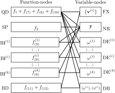
Figure 1. Representation of (6)-(12) as a factor-graph. Each function-node, and each variable-node, is labeled by two capital letters.

We interpret ADMM as an iterative scheme that operates on iterates that live on the edges/nodes of the factor-graph in Figure 1, similar to the approaches in (Derbinsky et al., 2013b; Derbinsky et al., 2013a; Hao et al., 2016). The function-nodes have the following labels: quadratic (QP), sparse (SP), bi-linear (${\text{BI}}^{(1)},\dots,{\text{BI}}^{({k})}$), and bound (BD). The variable-nodes have the following labels: flux (FX), new reaction (NR), dual equilibrium (${\text{DE}}^{(1)},\dots,{\text{DE}}^{({k})}$), and dual bound (DB). Each edge (function-node, variable-node), such as $({\text{BD}},{\text{DE}}^{(i)})$, has two associated iterates: a primal iterate ${\Psi}$ and a dual iterate ${\Xi}$. Both iterates are vectors whose dimension matches the variable in the variable-node that they connect to. Each edge also has an associated parameter ${\rho}>0$. For example, the dual iterate and parameter associated with the edge $({\text{BD}},{\text{DE}}^{(i)})$ are ${\Xi}_{{\text{BD}},{\text{DE}}^{(i)}}$ (dimension ${m}$) and ${\rho}_{{\text{BD}},{\text{DE}}^{(i)}}$ respectively. Each variable-node has one associated iterate: a consensus iterate ${\Gamma}$ whose dimension matches the variable associated with the variable-node. For example, the consensus iterate associated with node DB is ${\Gamma}_{\text{DB}}$ (dimension $2{k}{n}$).

Essential to ADMM is the concept of a proximal operator (PO) of a function $f:\mathbb{R}^{s}\mapsto\mathbb{R}$ with parameter ${\rho}$. This is a map ${\mathbf{Prox}}_{f,{\rho}}:\mathbb{R}^{s}\mapsto\mathbb{R}^{s}$ that takes as input ${{\bf n}}\in\mathbb{R}^{s}$ and outputs

(13) $${\mathbf{Prox}}_{f,{\rho}}({{\bf n}})\in\arg\min_{{\bf w}\in\mathbb{R}^{s}}f({\bf w})+\frac{{\rho}}{2}\|{{\bf n}}-{\bf w}\|^{2}_{2}.$$

We denote the POs for the function in each function-node as ${\mathbf{Prox}}_{{\text{QP}}}$, ${\mathbf{Prox}}_{{\text{SP}}}$, ${\mathbf{Prox}}_{{\text{BI}}}$, and ${\mathbf{Prox}}_{{\text{BD}}}$ respectively. All POs have uniquely defined outputs.

Given this setup, the over-relaxed distributed-consensus ADMM algorithm leads directly to Algorithm 1, which is the basis of BIG-BOSS. In Algorithm 1, if $Y$ is a variable-node, $\partial Y$ represents all edges incident on $Y$. Similarly, if $X$ is a function-node, $\partial X$ represents all edges incident on $X$. Note that each for-loop in Algorithm 1 can be computed in parallel.

Algorithm 1 Algorithm for BIG-BOSS

1:while $!$stopping criteria do

2:     for $E=(X,Y)\in\text{edges of factor-graph}$ do

3:         ${\Xi}_{E}\leftarrow{\Xi}_{E}+{\alpha}({\gamma}{\Psi}_{E}-{\Gamma}_{Y}+(1-{\gamma}){\Gamma}_{Y}^{\text{old}})$

4:     end for

5:     for $X\in\text{function-nodes of factor-graph}$ do

6:         $\{{\Psi}_{E}\}_{E\in\partial X}\leftarrow{\mathbf{Prox}}_{X,{\rho}_{X}}(\{{\Gamma}_{Y}-{\Xi}_{E}\}_{E\in\partial X})$

7:     end for

8:     for $Y\in\text{variable-nodes of factor-graph}$ do

9:         ${\Gamma}_{Y}^{\text{old}}\leftarrow{\Gamma}_{Y}$

10:         ${\Gamma}_{Y}\leftarrow(1-{\gamma}){\Gamma}_{Y}+\frac{\sum_{E\in\partial Y}{\rho}_{E}({\gamma}{\Psi}_{E}+{\Xi}_{E})}{\sum_{E\in\partial Y}{\rho}_{E}}$

11:     end for

12:end while

The rate of convergence of ADMM is influenced by the multiple ${\rho}$’s, ${\gamma}$, and ${\alpha}$, and there are various methods for choosing good values or adapting them while ADMM is running (He et al., 2000; Boyd et al., 2011; Derbinsky et al., 2013b; Xu et al., 2016, 2017; Stellato et al., 2017; Wohlberg, 2017). As described in Section 4.6, we implement the residual balancing method (Stellato et al., 2017). Although this scheme is not provably optimal, the algorithm converges very quickly in practice, and the BIG-BOSS user need not worry about tuning in general. In BIG-BOSS, all of the ${\rho}$’s corresponding to edges incident on the same function-node $X$ in the factor-graph have the same value, ${\rho}_{X}$, throughout ADMM’s execution. See Section 4.6 for more details. In this work, we run ADMM until all of the iterates are identical between iterations to a numerical absolute tolerance of $10^{-9}$. This is our stopping criterion.

Most updates in Algorithm 1 are linear. The exceptions are updates involving POs, which require solving (13) for different functions $f$. A vital part of our work was to find efficient solvers for each PO. Our decomposition of problem (6)-(12) into the specific form of Figure 1 is not accidental. It leads to a very small number of POs, all of which can be evaluated quickly. (${\mathbf{Prox}}_{{\text{QP}}}$ amounts to solving a linear system, and the others can be computed in closed form.) We expand on this in the next sections.

4.1. Proximal operator for node QP

The function-node QP is a quadratic objective subject to some linear constraints. To explain how we compute ${\mathbf{Prox}}_{{\text{QP}}}$, we start by defining ${\bf w}^{(i)}=\{{{\bf v}^{(i)}},{\bm{\omega}^{(i)}},{\bm{\mu}}^{(i)},{\bm{\eta}}^{(i)},{\bf y}\}\in\mathbb{R}^{2({n}+{m})+{m}}$ for each condition $i$, writing

$$f_{1}(\{{\bf w}^{(i)}\})=\frac{1}{k}\sum^{{k}}_{i=1}\left\lVert{P^{(i)}}{\bf w}^{(i)}-{{\bf q}^{(i)}}\right\rVert_{2}^{2},$$

and writing the constraints $f_{\eqref{eq:bilinear_Li_1}}+f_{\eqref{eq:bilinear_Li_2}}+f_{\eqref{eq:dual_equals_primal}}<+\infty$ as ${C^{(i)}}{\bf w}^{(i)}={{\bf e}^{(i)}}$, $\forall i\in\{1,\dots,{k}\}$, where

$${P^{(i)}}=\begin{bmatrix}{F^{(i)}}&0&0&0&0\end{bmatrix},\ {{\bf q}^{(i)}}=\begin{bmatrix}{{\bf\tilde{v}}^{(i)}}\end{bmatrix},$$

$${C^{(i)}}=\begin{bmatrix}{S}&0&0&0&{z^{(i)}}\\ 0&{S}^{T}\!&-I&I&0\\ {\bf c}^{T}\!&-{\bf b}^{T}\!&{{\bf l}^{(i)}}^{T}\!&-{{\bf u}^{(i)}}^{T}\!&0\end{bmatrix},\text{ and }{{\bf e}^{(i)}}=\begin{bmatrix}{{\bf b}^{(i)}}\\ {\bf c}\\ -{z^{(i)}}\end{bmatrix}.$$

Evaluating ${\mathbf{Prox}}_{{\text{QP}}}(\{{{\bf n}^{(i)}}\})$ for input vectors $\{{{\bf n}^{(i)}}\}\in\mathbb{R}^{2{k}({n}+{m})+{m}}$ now amounts to finding the unique minimizer of a strongly convex quadratic program with linear constraints, namely,

$$\min_{\{{\bf w}^{(i)}\}\in\mathbb{R}^{2k({n}+{m})+{m}}}\frac{1}{k}\sum^{{k}}_{i=1}\|{P^{(i)}}{\bf w}^{(i)}-{{\bf q}^{(i)}}\|^{2}_{2}+\frac{{\rho}}{2}\sum^{{k}}_{i=1}\|{\bf w}^{(i)}-{{\bf n}^{(i)}}\|^{2}_{2}$$

$$\text{ subject to }{C^{(i)}}{\bf w}^{(i)}={{\bf e}^{(i)}},\forall i\in\{1,\dots,{k}\}.$$

We find this unique minimizer by solving a linear system obtained from the KKT conditions. We then have ${k}$ linear systems that are coupled by the variable ${\bf y}$ that is common to each ${\bf w}^{(i)}$. We can write each linear system in block form as

(14) $$\begin{bmatrix}\frac{2}{k}{P^{(i)}}^{T}\!{P^{(i)}}+{\rho}I&{C^{(i)}}^{T}\\ {C^{(i)}}&0\end{bmatrix}\begin{bmatrix}{\bf w}^{(i)}\\ {{\bf\lambda}^{(i)}}\end{bmatrix}=\begin{bmatrix}\frac{2}{k}{P^{(i)}}^{T}\!{{\bf q}^{(i)}}+{\rho}{{\bf n}^{(i)}}\\ {{\bf e}^{(i)}}\end{bmatrix},$$

where ${{\bf\lambda}^{(i)}}$ is the Lagrange multiplier for the linear constraints ${C^{(i)}}{\bf w}^{(i)}={{\bf e}^{(i)}}$. Finally, we stack the ${k}$ linear systems into one large linear system. For numerical stability reasons, we add $-\beta I$, $\beta=10^{-12}$, to the system’s matrix. This ensures a unique solution. As described in Section 4.5, we also implemented a preconditioner for this linear system to improve its condition number.

To solve the linear system, we compared two different numerical libraries. One is the C library UMFPACK, which we called from Fortran using the Fortran 2003 interface in mUMFPACK 1.0 (Hanyk, [n. d.]). The other is the symmetric indefinite solver MA57 (Duff, 2004) from HSL (HSL, 2013). For both solvers, the symbolic factorization needs to be computed only once. When $\rho$ is updated, only the numerical factorization is recomputed. As other groups have reported (Gould et al., 2007), we found that MA57’s solve phase was faster than UMFPACK’s. We therefore used MA57 for all results in this study.

4.2. Proximal operator for node DB

Observe that the constraint $f_{\eqref{eq:bilinear_Li_3}}+f_{\eqref{eq:bilinear_Li_4}}<+\infty$ is equivalent to $3{k}$ constraints of the type ${{\bf e}}^{(i,j)}\leq{\bf w}^{(i,j)}\leq{{\bf q}}^{(i,j)}$ for some constant vectors ${{\bf e}}^{(i,j)},{{\bf q}}^{(i,j)}\in\mathbb{R}^{{n}}$: one for each condition $i$ and each of the variables ${{\bf v}^{(i)}}$ (for index $j=1$), ${\bm{\mu}}^{(i)}$ ( for index $j=3$), and ${\bm{\eta}}^{(i)}$ (for index $j=4$). Hence, computing ${\mathbf{Prox}}_{{\text{DB}}}(\{{{\bf n}}^{(i,j)}\})$ for some input $\{{{\bf n}}^{(i,j)}\}\in\mathbb{R}^{3{k}{n}}$ amounts to solving $3{k}$ independent problems

$$\min_{{\bf w}^{(i,j)}\in\mathbb{R}^{{n}}}\frac{\rho}{2}\left\lVert{\bf w}^{(i,j)}-{{\bf n}}^{(i,j)}\right\rVert_{2}^{2}\text{\ subject to\ }{{\bf e}}^{(i,j)}\leq{\bf w}^{(i,j)}\leq{{\bf q}}^{(i,j)}.$$

This problem has a unique minimizer given explicitly by

$${\bf w}^{(i,j)}=\min\{{{\bf q}}^{(i,j)},\max\{{{\bf e}}^{(i,j)},{{\bf n}}^{(i,j)}\}\},$$

where $\min$ and $\max$ are taken component-wise.

4.3. Proximal operator for node SP

The PO for node SP, which has $f_{2}({\bf w})=\delta\|{\bf w}\|_{1}$, requires finding the minimizer of

$$\min_{{\bf w}\in\mathbb{R}^{{m}}}\frac{\rho}{2}\left\lVert{\bf w}-{{\bf n}}\right\rVert_{2}^{2}+{\delta}\left\lVert{\bf w}\right\rVert_{1}.$$

This minimizer is ${\bf w}=\mathbf{S}_{{\delta}/\rho}({{\bf n}})$, where $\mathbf{S}_{t}(\cdot)$ is the element-wise soft-thresholding operator (Boyd et al., 2011) defined, for input scalar $x$, as

(15) $$S_{t}(x)=\begin{cases}0,&\text{if}\ |x|\leq t\\ \text{sign}(x)(|x|-t),&\text{otherwise}.\end{cases}$$

4.4. Proximal operator for node ${\text{BI}}^{(i)}$

The $i$th bilinear proximal operator ${\mathbf{Prox}}_{{\text{BI}}^{(i)}}$ receives input vectors ${{\bf n}},{{\bf n}^{(i)}}\in\mathbb{R}^{{m}}$, and outputs the minimizer of

(16) $$\min_{{\bf y},{\bf w}^{(i)}\in\mathbb{R}^{{m}}}\quad \frac{\rho}{2}\left\lVert{\bf y}-{{\bf n}}\right\rVert^{2}_{2}+\frac{\rho}{2}\left\lVert{\bm{\omega}^{(i)}}-{{\bf n}^{(i)}}\right\rVert^{2}_{2}$$

(17) subject to $${\bf y}^{T}\!{\bm{\omega}^{(i)}}\geq{{d}^{(i)}}.$$

To solve this problem, we consider two cases. If ${{\bf n}^{(i)}}^{T}\!{{\bf n}}\geq{{d}^{(i)}}$, we know that the minimizer is $({\bf y},{\bf w}^{(i)})=({{\bf n}},{{\bf n}^{(i)}})$. Otherwise, we know that the constraint (17) is active, and we compute the minimizer from among the set of solutions of the KKT conditions for the (now constrained) problem. The KKT conditions are

$$\rho{\bf y}-\rho{{\bf n}}-{{\bf\lambda}}{\bm{\omega}^{(i)}}=0,\ \rho{\bm{\omega}^{(i)}}-\rho{{\bf n}^{(i)}}-{{\bf\lambda}}{\bf y}=0,\ {\bf y}^{T}\!{\bm{\omega}^{(i)}}={{d}^{(i)}},$$

where ${{\bf\lambda}}$ is the dual variable for the constraint ${\bf y}^{T}\!{\bm{\omega}^{(i)}}\geq{{d}^{(i)}}$. By defining $x={{\bf\lambda}}/{\rho}$ and reformulating the KKT system, we arrive at the following quartic equation that determines the value of ${{\bf\lambda}}$:

$${{d}^{(i)}}x^{4}+(-2{{d}^{(i)}}-{{\bf n}}^{T}\!{{\bf n}^{(i)}})x^{2}+({{\bf n}}^{T}\!{{\bf n}}+{{\bf n}^{(i)}}^{T}\!{{\bf n}^{(i)}})x$$

(18) $$\hbox{}+({{d}^{(i)}}-{{\bf n}}^{T}\!{{\bf n}^{(i)}})=0.$$

We solve this quartic equation in closed form, using the Quartic Polynomial Program Fortran code (Morris Jr, 1993; Carmichael, [n. d.]). For each real root, $x$, we compute ${\bf y}$ and ${\bm{\omega}^{(i)}}$ as

(19) $${\bf y} =\frac{{{\bf n}}-{x}{{\bf n}^{(i)}}}{1-{x}^{2}},\quad{\bm{\omega}^{(i)}}=\frac{{{\bf n}^{(i)}}-{x}{{\bf n}}}{1-{x}^{2}},$$

and we keep the solution that minimizes the objective function (16).

4.5. Preconditioner

The convergence rate of the ADMM can be improved by preconditioning the data matrices associated with the node QP (Stellato et al., 2017; Takapoui and Javadi, 2016).

We use the Ruiz equilibration method (Ruiz, 2001) to compute positive definite diagonal matrices, ${Q}$ and ${R}$, with which we scale all of the variables $\{{\bf w}^{(i)}=\{{{\bf v}^{(i)}},{\bm{\omega}^{(i)}},{\bm{\mu}}^{(i)},{\bm{\eta}}^{(i)},{\bf y}\}\}$ in our formulation, as well as the constraints ${C^{(i)}}{\bf w}^{(i)}={{\bf e}^{(i)}}\forall i$, associated with the node QP. The new scaled variables are defined through the change of variable ${\bf w}^{(i)}\rightarrow{Q}{{\bf w}^{(i)}}$, and the new constraints then transform as ${C^{(i)}}{{\bf w}^{(i)}}={{\bf e}^{(i)}}\rightarrow{R}{C^{(i)}}{Q}{{\bf w}^{(i)}}={R}{{\bf e}^{(i)}}\forall i$. Note that all of the copies of ${\bf y}$ inside each ${\bf w}^{(i)}$ get scaled exactly in the same way.

This scaling affects the different proximal operators in different ways. The node QP, that requires computing ${\mathbf{Prox}}_{{\text{QP}}}(\{{{\bf n}^{(i)}}\})$, now requires solving a modified version of (14), namely, the following system of linear equations (coupled by ${\bf y}$),

$$\begin{bmatrix}{Q}\frac{2}{k}{P^{(i)}}^{T}\!{P^{(i)}}{Q}+{\rho}I&{Q}{C^{(i)}}^{T}\!{R}\\ {R}{C^{(i)}}{Q}&0\end{bmatrix}\begin{bmatrix}{{\bf w}^{(i)}}\\ {{{\bf\lambda}^{(i)}}}\end{bmatrix}=\begin{bmatrix}{Q}\frac{2}{k}{P^{(i)}}^{T}\!{{\bf q}^{(i)}}+{\rho}{{{\bf n}^{(i)}}}\\ {R}{{\bf e}^{(i)}}\end{bmatrix}.$$

For ${\mathbf{Prox}}_{{\text{DB}}}(\{{{\bf n}}^{(i,j)}\})$, let ${Q}^{(j)}$, $j=1,3,4$, be the diagonal block of ${Q}$ that scales the variables ${{\bf v}^{(i)}}$ ($j=1$), ${\bm{\mu}}^{(i)}$ ($j=3$), and ${\bm{\eta}}^{(i)}$ ($j=4$). We now solve $3k$ problems of the type

(20) $$\min_{{\bf w}^{(i,j)}\in\mathbb{R}^{{n}}}\frac{\rho}{2}\left\lVert{{\bf w}^{(i,j)}}-{{{\bf n}}^{(i,j)}}\right\rVert_{2}^{2}\text{\ subject to\ }$$

(21) $${{Q}^{(j)}}^{-1}{{\bf e}}^{(i,j)}\leq{{\bf w}^{(i,j)}}\leq{{Q}^{(j)}}^{-1}{{\bf q}}^{(i,j)},$$

which has a unique minimizer

$${{\bf w}^{(i)}}=\min\{{{Q}^{(j)}}^{-1}{{\bf q}}^{(i,j)},\max\{{{Q}^{(j)}}^{-1}{{\bf e}}^{(i,j)},{{{\bf n}}^{(i,j)}}\}\}.$$

For the node SP, let ${Q}^{(5)}$ be the diagonal block of ${Q}$ that scales the variable ${\bf y}$. The new ${\mathbf{Prox}}_{{\text{SP}}}({{\bf n}})$ now outputs

$${{\bf w}}=\mathbf{S}_{{{Q}^{(5)}}^{-1}{\delta}/\rho}({{\bf n}}),$$

where, for the $r$th component of ${{\bf n}}$, we use the $r$th diagonal element of ${{Q}^{(5)}}^{-1}{\delta}/\rho$ in the operator $\mathbf{S}$, that is applied component-wise.

For the $i$th bilinear proximal operator ${\mathbf{Prox}}_{{\text{BI}}^{(i)}}({{\bf n}},{{\bf n}^{(i)}})$, we now solve

$$\operatorname*{\arg\min}_{{{\bf y}},{{\bm{\omega}^{(i)}}}\in\mathbb{R}^{{m}}}\quad \frac{\rho}{2}\left\lVert{{\bf y}}-{{{\bf n}}}\right\rVert^{2}_{2}+\frac{\rho}{2}\left\lVert{{\bm{\omega}^{(i)}}}-{{{\bf n}^{(i)}}}\right\rVert^{2}_{2}$$

subject to $${{\bf y}}^{T}\!{Q}^{(5)}{Q}^{(2)}{{\bm{\omega}^{(i)}}}\geq{{d}^{(i)}},$$

where ${Q}^{(2)}$ is the diagonal block of ${Q}$ that scales the variable ${\bm{\omega}^{(i)}}$. We modify the Ruiz equilibration method such that ${Q}^{(5)}{Q}^{(2)}=constant\times I$, and hence we can solve this PO using the same method as before.

4.6. Adaptive penalty

Our ADMM scheme allows for one ${\rho}$ per each edge in the factor-graph in Fig. 1. In BIG-BOSS, these ${\rho}$’s are chosen automatically, such that a user does not need to worry about tuning. All of the ${\rho}$’s associated with edges incident on the same function-node have the same value. Hence, we refer to the different ${\rho}$’s by their respective PO. We update the ${\rho}$’s for each PO dynamically every $1000$ iterations using the residual balancing method (Boyd et al., 2011), which we now explain.

Similar to (Stellato et al., 2017; Wohlberg, 2017), we define the vector of relative primal residuals at iteration $10^{3}\times t$, and for any proximal operator $X$, as

$$r_{\text{prim}}(t)=\frac{\{{\Psi}_{E}(t)-{\Gamma}_{Y}(t)\}_{E:E=(X,Y)\in\partial X}}{\max\{\{\max\{|{\Psi}_{E}(t)|,|{\Gamma}_{Y}(t)|\}\}_{E:E=(X,Y)\in\partial X}\}},$$

where, we recall, $\partial X$ are all the edges incident on node $X$.

The vector of relative dual residuals for the proximal operator $X={\text{QP}}$ at iteration $10^{3}\times t$ is defined as follows. Let

$$C_{1} =\max^{k}_{i=1}\left\|\frac{2}{k}{P^{(i)}}^{T}\!{P^{(i)}}\{{\Psi}_{E}(t+1)\}_{E\in\partial X}\right\|_{\infty},$$

$$C_{2} =\|\{{\Xi}_{E}(t+1)\}_{E\in\partial X}\|_{\infty},\text{ and }C_{3}=\max^{{k}}_{i=1}\left\|-\frac{2}{k}{P^{(i)}}^{T}\!{{\bf q}^{(i)}}\right\|_{\infty}.$$

We define

$$r_{\text{dual}}(t+1)=\frac{\{{\Gamma}_{Y}(t+1)-{\Gamma}_{Y}(t)\}_{Y:(X,Y)\in\partial X}}{\max\{C_{1},C_{2},C_{3}\}}.$$

If $X$ is a PO other than QP, we define

$$r_{\text{dual}}(t+1)=\frac{\{{\Gamma}_{Y}(t+1)-{\Gamma}_{Y}(t)\}_{Y:(X,Y)\in\partial X}}{C_{2}},$$

since $C_{1}$ and $C_{3}$ do not exist when $X$ is not QP.

The ${\rho}$ update rule is then defined as follows. Once the $\infty$-norm of both the primal and the dual residuals falls below a threshold of $10^{-3}$, we start updating ${\rho}$ as

$${\rho}(t+1)=\max\{10^{-3},\min\{10^{3},\tilde{{\rho}}(t+1)\}\}$$

where

$$\tilde{{\rho}}(t+1)=\begin{cases}\tau{\rho}(t)&\text{if}\ \left|\ln\left(\|r_{\text{prim}}(t)\|_{\infty}/\|r_{\text{dual}}(t)\|_{\infty}\right)\right|\geq\ln(\eta),\\ \rho(t)&\text{otherwise},\end{cases}$$

where $\tau=\sqrt{\|r(t)_{\text{prim}}\|_{\infty}/\|r(t)_{\text{dual}}\|_{\infty}}$ and $\eta>0$, which in this study we set to $2$, is a threshold to prevent the ${\rho}$ from changing too frequently. Note that a frequently-changing ${\rho}$ requires many numerical re-factorization for solving the linear system in the node QP. Furthermore, a frequently-changing ${\rho}$ might compromise the convergence of the ADMM.

4.7. Step size

The step size ${\alpha}$ in Algorithm 1 can be adjusted to speed up convergence. We used a default step size of 1.0 for all problems. If the problem did not converge to the desired tolerance within 2 million iterations, we re-ran the problem with a simple step size heuristic. We use ${\alpha}=1$ for 10,000 iterations, ${\alpha}=0.1$ for 100,000 iterations, then ${\alpha}=0.001$ until convergence, or the iteration limit is reached.

5. Experimental results

5.1. BOSS versus BIG-BOSS

We compare BIG-BOSS with BOSS in terms of running speed, and accuracy. To make a valid comparison, we set ${k}=1$ and ${\delta}=0$, such that BIG-BOSS is doing the same inference as BOSS (Gianchandani et al., 2008). BOSS requires choosing an off-the-shelf nonlinear programming solver, we choose IPOPT (Wächter and Biegler, 2006) (v24.7.1), an open-source, interior-point solver used to solve large-scale nonlinear programs.

We generate synthetic flux measurements, ${\bf\tilde{v}}$, using the latest metabolic network of E. coli (Monk et al., 2017) called iML1515. This network has $1,877$ metabolites and $2,712$ reactions. We then hide one goal reaction from the network, ${\bf y}$, and try to infer it from flux data.

Using a single CPU core (Intel i7, $3.4$GHz), BOSS is able to learn ${\bf y}$ for this model in $13.3$ seconds (wall time) using IPOPT to primal and dual residuals of $1.05\times 10^{-11}$ and $7.23\times 10^{-11}$. Using the same CPU core, BIG-BOSS is able to learn ${\bf y}$ in $113$ seconds to primal and dual residuals of $2.73\times 10^{-10}$ and $6.63\times 10^{-10}$. In Appendix A.3, we report the run-time for other accuracy values. Although BIG-BOSS is slower than BOSS, it is still fast, and, more importantly, allows $k>1,\delta>0$, and the use of multiple cores for large models.

Now we look at how well the recovered reaction coefficients ${\bf y}$ compare to the true coefficients that we hide, both in BOSS and BIG-BOSS. We do so by (i) directly comparing the ground truth with the recovered ${\bf y}$, as well as, (ii) using the recovered ${\bf y}$ to predict measured fluxes (training fluxes).

For BOSS, the recovered goal reaction coefficients ${\bf y}$ closely resemble the true reaction coefficients, with Spearman rank correlation, $r^{\text{Spearman}}=0.996$ (Fig. 2a). With the recovered ${\bf y}$ back into the model, we then solve (1) to simulate fluxes. For BOSS, the estimated goal reaction has zero flux, resulting in simulated fluxes that do not resemble the training fluxes (Fig. 2c). To help BOSS, we make ${\bf y}$ sparse by zeroing coefficients with absolute value smaller than a fixed threshold $\theta$. Since this cannot be done in a real setting, it shows a limitation in BOSS. We tested thresholds between $0$ to $1$ and found that values between $10^{-3}$ to $10^{-1}$ result in accurate flux predictions ($0.98\leq R^{2}\leq 1.0$).

We perform the same experiment using BIG-BOSS, which estimates ${\bf y}$ with $r^{\text{Spearman}}=0.871$ (Fig. 2b). Fluxes predicted using this new reaction are accurate on the training data to $R^{2}=0.994$ without zeroing additional coefficients (Fig. 2d).

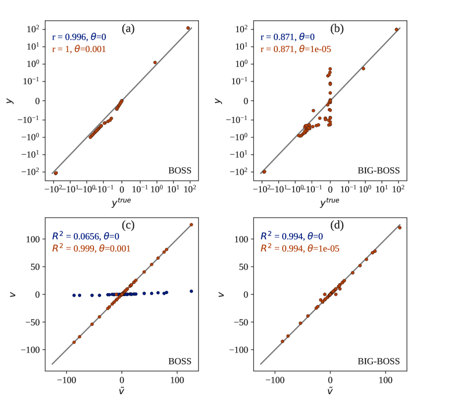
Figure 2. Performance of BOSS and BIG-BOSS. Coefficients of ${\bf y}$ estimated using BOSS (a) and BIG-BOSS (b) compared against true coefficients. Fluxes predicted using the goal reaction estimated by BOSS (c) and BIG-BOSS (d) compared against training fluxes ${\bf\tilde{v}}$. $R^{2}$: coefficient of variation. $r$: Spearman rank correlation. $\theta$: threshold for zeroing out elements of ${\bf y}$ smaller than $\theta$.

5.2. Experiments with $75$ large-scale models

We test our algorithm’s performance on $75$ large-scale metabolic networks in the BiGG database (King et al., 2015). Model sizes ranged from $95$ to $10,600$ reactions and $72$ to $5,835$ metabolites. The median model size is $2,727$ reactions and $1,942$ metabolites. For each model, we generate synthetic training fluxes by solving Problem (1) using the existing cellular goal reaction. To generate test data, we do as above but in a different simulated nutrient environment. This is accomplished by changing the bounds ${\bf l}$ and ${\bf u}$ on nutrient transport reactions. Our algorithm then receives as input the training fluxes, the bounds, and an incomplete stoichiometric matrix, which is missing the column corresponding to the “ground truth” cellular goal reaction that we want to estimate.

We evaluate our algorithm’s performance based on three metrics: (i) how well the estimated reaction allows to predict training fluxes, (ii) how well the estimated reaction allows to predict testing fluxes, and (iii) how close the estimated reaction coefficients are to the ground truth coefficients. To evaluate metrics (i) and (ii), we insert the estimated reaction into the metabolic network, having first removed the true goal reaction, and then simulate fluxes.

Based on the coefficient of determination ($R^{2}$) between measured and predicted fluxes, both training and test performances were high (median $R^{2}$ of $0.993$ and $0.977$) (Table 2). To assess the significance of these $R^{2}$ values, we compare them with fluxes generated from $1,000$ random goal reactions. These random goal reactions are obtained by randomly shuffling the coefficients of the ground truth coefficients. We say that the $R^{2}$ based on our algorithm is significant if it exceeds 95% of the $R^{2}$ values that were computed using the 1,000 random goal reactions. Overall, $R^{2}$ values are significant for $70.1\%$ of the models for training data and $67.2\%$ of the models for test data (Table 2). The ground truth goal reaction is recovered accurately: across $75$ models, the median Pearson correlation was $1.0$ (Table 3). The Spearman rank correlation was lower, with median $0.48$. The fact that predicted fluxes are accurate indicates that metabolic flux predictions are relatively insensitive to the precise recovery of the true coefficients in ${\bf y}$.

In biological experiments, the majority of fluxes are unmeasured, so $50\%$ missing flux measurements is common (Antoniewicz, 2015). We test the effect of missing flux measurements by randomly removing $10$% and $50$% of measurements, repeated five times. The main consequence of missing measurements is that recovering the ground truth goal is more difficult. With $10\%$ and $50\%$ of missing measurements, median Pearson correlations of $-0.023$ and $0.0012$ are obtained (Table 2). The accuracy of predicted fluxes also deteriorate when measurements are missing (Table 2). However, depending on which reactions are measured, fluxes can be predicted with $R^{2}>0.90$ for $6.67\%$ of the cases with $10\%$ of missing measurements, and for $3.16\%$ of the cases with $50\%$ of missing measurements, in the case of test data. This result shows that certain fluxes are more important than others, and that BIG-BOSS can recover goal reactions when those important fluxes are measured.

Table 2. Performance for $75$ BiGG models. $R^{2}$: coefficient of determination. By ‘significant’ we mean that the $R^{2}$ based on our algorithm’s goal reaction exceeds 95% of the $R^{2}$ values that are based on 1,000 random goal reactions.

	% missing	$R^{2}$		% cases,	% cases,
Data	fluxes	mean	median	$R^{2}>0.90$	significant
Train	0.0	0.711	0.993	63.8	70.1
	10.0	-6.89	0.56	12.2	19.7
	50.0	-38.9	0.604	4.98	6.45
Test	0.0	0.666	0.977	59.4	67.2
	10.0	-4.7	0.33	6.67	15
	50.0	-29.2	0.431	3.16	6.56

Table 3. Goal reaction recovery accuracy for 75 BiGG models.

% missing	Metric	min	max	mean	median
fluxes
0.0	Pearson	0.021	1	0.96	1
	Spearman	0.1	0.76	0.48	0.48
10.0	Pearson	-0.74	1	0.063	-0.023
	Spearman	-0.12	0.9	0.59	0.63
50.0	Pearson	-0.92	0.82	-0.032	0.0012
	Spearman	-0.27	0.76	0.38	0.4

5.3. Effect of multiple data types

Next, we investigate if including data types other than metabolic fluxes can improve reaction estimation. In particular, the concentration of over $95\%$ of cell proteins and transcripts (RNA) can be measured (Schmidt et al., 2016). These data types have been used to identify statistically enriched biological functions (Hart et al., 2015) but not to estimate reactions. Thus, to include protein concentrations in our algorithm, we extend (1), similar to (Beg et al., 2007). (Details in Supplement A.1.)

We estimated goal reactions with three different data sets: only metabolic fluxes, only proteins, and both. To reflect realistic data, we include only metabolic fluxes for central metabolism, and include all proteins—this is achievable using proteomics, or with RNA sequencing where RNA is used to estimate protein concentrations. We then use the estimated goal reaction to predict all metabolic fluxes and protein concentrations (including values not seen by the algorithm) in left-out conditions to assess the test performance.

When only metabolic fluxes are provided, the prediction accuracy is low (mean $R^{2}=0.281$) (Table 4). When only proteins are provided, the accuracy is even lower (mean $R^{2}=-16.4$). One reason for the low accuracy is that protein concentrations are not always directly proportional to flux—they only provide an upper bound. When both fluxes and proteins are provided, the average test accuracy is $R^{2}=0.567$, which is double the accuracy with only flux measurements.

Table 4. Test performance of flux and protein predictions given different coverage of protein and flux measurements. Coverage refers to the percentage of fluxes or proteins that are measured and used as input to BIG-BOSS.

Coverage (%)		$R^{2}$
Flux	Protein	mean	min	max
57	100	0.567	0.108	0.77
57	0	0.281	0.225	0.322
0	100	-16.375	-23.556	-11.293

5.4. Multi-core speedup

Problem (5) can grow rapidly in size and can benefit from parallel computing. BOSS cannot exploit parallel computational resources, but BIG-BOSS can. We thus tested how BIG-BOSS scales with multiple processors, using the same metabolic network as in Section 5.1. To maximize parallelism, we implemented a fine-grained version of our algorithm, similar to (Hao et al., 2016). The fact that we are using ADMM is important to achieve this. This implementation involves splitting node QP: one for every constraint. By combining this fine-grained version of QP with BD and BI, we have our fine-grained BIG-BOSS. This implementation of BIG-BOSS gave 1.6$\times$ speedup with 2 CPUs, and 7$\times$ speedup with 64 CPUs (Fig. 3). With ${k}=2$ the speedup was greater, achieving $8\times$ with 32 and 64 CPUs.

In these experiments, we did not perform preconditioning or adaptive penalty to prevent factors besides CPU count from affecting speed. To parallelize our code, we used OpenACC and the PGI compiler 18.10. These tests were performed on Google Compute Engine virtual machines with 32-core (64-thread) Intel Xeon 2.30 GHz processors and 64 GB RAM.

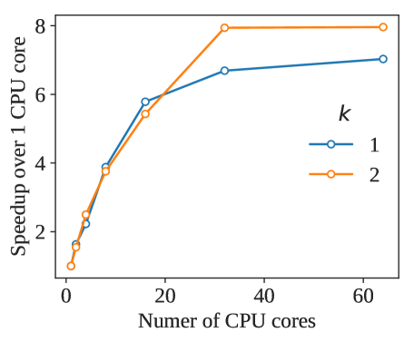
Figure 3. Speedup with multiple CPU cores for number of conditions ${k}=1$ and $2$ using the fine-grained implementation of BIG-BOSS.

6. Conclusion

In this work, we addressed the problem of estimating cellular goal reactions from measured fluxes in the context of constraint-based modeling of cell metabolism. This problem was previously addressed by the BOSS algorithm (Gianchandani et al., 2008), which successfully demonstrated the viability of this approach on a model of Saccharomyces cerevisiae central metabolism composed of 60 metabolites and 62 reactions. Here, we developed a new method that extends BOSS and demonstrates its performance on 75 metabolic networks having up to 10,600 reactions and 5,835 metabolites.

Our method successfully estimated goal reactions that enabled accurate prediction of metabolic fluxes in new nutrient environments (median coefficient of determination, $R^{2}=0.98$). Furthermore, the stoichiometric coefficients of the estimated reactions matched those of the ground truth reactions that were used to generate the training fluxes (median Pearson correlation, $r=0.96$).

As with the original BOSS, our algorithm involves a nonconvex optimization problem with bilinear constraints. ADMM is an efficient approach for solving problems with many bilinear constraints, and more generally, nonconvex quadratic constraints (Huang and Sidiropoulos, 2016). For our problem, the number of bilinear constraints can be large, as it increases with the number of conditions in the data. Besides scalability, BIG-BOSS allows for regularization, modularity—enabling extensions, and can use multiple data types (fluxes and protein concentrations), which improves prediction accuracy.

Genome-scale metabolic network models have been invaluable in numerous studies including infectious disease and cancer metabolism (Bordbar et al., 2014). The success of these studies depends on the availability of a reaction representing cellular goals. For many important cellular systemss, such as human tissue or microbiomes, such reactions are still challenging to determine experimentally (Feist and Palsson, 2016). Our study shows that a data-driven approach for cellular goal estimation is promising. This approach is most effective when we have high coverage flux measurements or complementary data types, such as flux measurements for parts of the network and protein or RNA abundance measurements for most of the metabolic genes. BIG-BOSS is thus suited for analyzing large gene expression data sets, e.g., from cancer tissue. BIG-BOSS is available at https://github.com/laurenceyang33/cellgoal.

7. Acknowledgements

This work was supported by the NIH grants 2R01GM057089 and 1U01AI124302, NSF grant IIS-1741129, and Novo Nordisk Foundation grant NNF10CC1016517.

Appendix A Details for reproducibility

A.1. Model formulation including proteins

Our model formulation for including protein concentrations is based on (Beg et al., 2007) and (Lloyd et al., 2018). First, we denote ${\bf p}$ as the vector of protein concentrations, whose length is the number of proteins in the metabolic network. Each protein has a molecular weight, which is stored in ${\bf a}$. One or more proteins combine to form enzyme complexes, ${\bf e}$, which are ultimately the molecules that catalyze metabolic reactions. The rate of a metabolic reaction is limited by the catalytic efficiency of an associated enzyme and that enzyme’s concentration. Since multiple enzymes can sometimes catalyze the same reaction, we have a matrix of catalytic efficiencies, ${K}$ mapping reactions to all possible enzymes. The total protein mass of a cell, ${t}$, can be measured, and this quantity imposes an upper bound on the sum of individual protein concentrations multiplied by their molecular weights, ${\bf a}$. Finally, each protein can be part of one or more enzyme complexes, and each enzyme complex is comprised of a fixed number of a particular protein. This protein to enzyme mapping is encoded in the matrix ${E}$.

By adding these relationships to $\eqref{eq:FBA}$, we have the following linear problem:

(22) $$\begin{split}\max_{{\bf v},{\bf p},{\bf e}}\quad&{\bf c}^{T}\!{\bf v}+{\bf f}^{T}\!{\bf p}\\ \text{\ subject to\ }\quad&{S}{\bf v}={\bf b},\\ &{\bf v}-{K}{\bf e}+{\bf\sigma}^{(1)}=0,\\ &{\bf a}^{T}\!{\bf p}+{\bf\sigma}^{(2)}=t,\\ &{E}{\bf e}-{\bf p}+{\bf\sigma}^{(3)}=0,\\ &{\bf l}\leq{\bf v}\leq{\bf u},\\ &{\bf p},{\bf e}\geq 0,\\ &{\bf\sigma}^{(j)}\geq 0,\forall j\in\{1,2,3\},\end{split}$$

where ${\bf f}$ is the cell’s relative importance of different proteins, and ${\bf\sigma}^{(j)}$ are non-negative slack variables.

By defining ${\bf w}=\{{\bf v},{\bf p},{\bf e},{\bf\sigma}^{(1)},{\bf\sigma}^{(2)},{\bf\sigma}^{(3)}\}$,

$$\bar{{S}}=\begin{bmatrix}{S}&0&0&0&0&0\\ I&0&-K&I&0&0\\ 0&-I&E&0&0&I\end{bmatrix},$$

$\bar{{\bf c}}=\{{\bf c},{\bf f}\}$, $\bar{{\bf l}}=\{{\bf l},0,0,0,0,0\}$, $\bar{{\bf u}}=\{{\bf u},+\infty,+\infty,+\infty\,+\infty,+\infty\}$, and $\bar{{\bf b}}=\{{\bf b},0,t,0\}$, we can write (22) as

(23) $$\max_{{\bf w}}\bar{{\bf c}}^{T}\!{\bf w}\text{\ subject to\ }\bar{{S}}{\bf w}=\bar{{\bf b}},\ \bar{{\bf l}}\leq{\bf w}\leq\bar{{\bf u}},$$

which is (1) with a change of variables. Therefore, BIG-BOSS can be applied directly to the problem with proteins and fluxes.

The ${K}$ matrix is typically not known fully. Here, we used a default value of $65$ second^-1, which are in units of enzyme turnover rate and represents an average catalytic efficiency for all enzymes in E. coli. Values for matrix ${E}$ were determined from the gene-protein-reaction mappings that are included with each metabolic model in the BiGG database (King et al., 2015). Without additional information we assumed that each complex requires one unit of each protein in the gene-protein mapping. For ${t}$, we chose a default value of 0.30, indicating that the model accounts for $30$% of the cell’s protein mass. For molecular weights ${\bf a}$, we used a default value of 77 kDa for every protein, based on the average molecular weight of proteins in E. coli. (Note that ${\bf a}$ can also be determined directly from the protein’s amino acid sequence.)

A.2. Online Resources

Code and documentation for BIG-BOSS are available at https://github.com/laurenceyang33/cellgoal. Detailed installation instructions are available there. Briefly, users will need a Fortran compiler, CMake, and a linear system solver. We tested our algorithm with both UMFPACK, which is part of SuiteSparse, and MA57 (Duff, 2004) from HSL (HSL, 2013). For parallel computing features, users will need OpenACC and the PGI Compiler. We have tested all code using PGI Community Edition version 18.10. In the code repository, we include test suites to run BIG-BOSS on metabolic network models that users can download from the BiGG database (King et al., 2015).

A.3. Details on solution time

We report details on the run time for BIG-BOSS when solving the problem shown in Fig. 2. Solutions having modest accuracy are found quickly, as is expected for ADMM (Fig. 4).

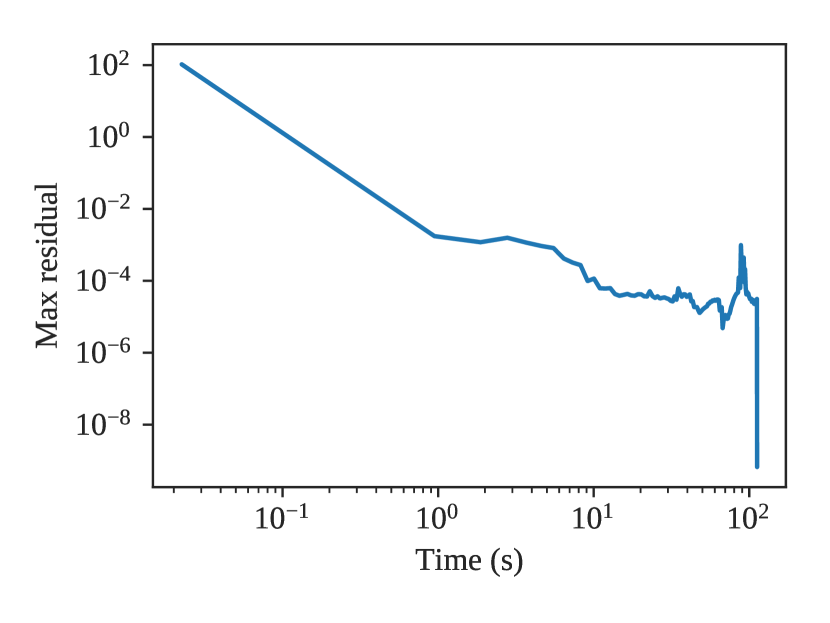
Figure 4. Maximum of primal and dual residuals versus the wall time of running BIG-BOSS.

References

- (1)
- Antoniewicz (2015) M. R. Antoniewicz. 2015. Methods and advances in metabolic flux analysis: a mini-review. J Ind Microbiol Biot 42, 3 (2015), 317–325.
- Bard (2013) J. F. Bard. 2013. Practical bilevel optimization: algorithms and applications. Vol. 30. Springer Science & Business Media.
- Beg et al. (2007) Q. K. Beg, A. Vazquez, J. Ernst, M. A. de Menezes, Z. Bar-Joseph, A.-L. Barabasi, and Z. N. Oltvai. 2007. Intracellular crowding defines the mode and sequence of substrate uptake by Escherichia coli and constrains its metabolic activity. Proc. Natl. Acad. Sci. USA 104 (2007), 12663–12668.
- Bento et al. (2013) J. Bento, N. Derbinsky, J. Alonso-Mora, and J. S. Yedidia. 2013. A message-passing algorithm for multi-agent trajectory planning. In Adv Neur In. 521–529.
- Bordbar et al. (2014) A. Bordbar, J. M. Monk, Z. A. King, and B. O. Palsson. 2014. Constraint-based models predict metabolic and associated cellular functions. Nat Rev Genet 15 (2014), 107–120.
- Boyd et al. (2011) S. Boyd, N. Parikh, E. Chu, B. Peleato, J. Eckstein, et al. 2011. Distributed optimization and statistical learning via the alternating direction method of multipliers. Foundations and Trends in Machine learning 3, 1 (2011), 1–122.
- Brunk et al. (2018) E. Brunk, S. Sahoo, D. C. Zielinski, A. Altunkaya, A. Dräger, et al. 2018. Recon3D enables a three-dimensional view of gene variation in human metabolism. Nat Biotechnol 36, 3 (2018), 272.
- Brynildsen et al. (2013) M. P. Brynildsen, J. A. Winkler, C. S. Spina, I. C. MacDonald, and J. J. Collins. 2013. Potentiating antibacterial activity by predictably enhancing endogenous microbial ROS production. Nat Biotechnol 31, 2 (2013), 160–165.
- Burgard and Maranas (2003) A. P. Burgard and C. D. Maranas. 2003. Optimization-based framework for inferring and testing hypothesized metabolic objective functions. Biotechnol Bioeng 82 (2003), 670–677.
- Carmichael ([n. d.]) R. L. Carmichael. [n. d.]. Public Domain Aeronautical Software. http://www.pdas.com. Accessed: 2018-08-12.
- Derbinsky et al. (2013b) N. Derbinsky, J. Bento, V. Elser, and J. S. Yedidia. 2013b. An improved three-weight message-passing algorithm. arXiv preprint arXiv:1305.1961 (2013).
- Derbinsky et al. (2013a) N. Derbinsky, J. Bento, and J. S. Yedidia. 2013a. Methods for integrating knowledge with the three-weight optimization algorithm for hybrid cognitive processing. arXiv preprint arXiv:1311.4064 (2013).
- Duff (2004) I. S. Duff. 2004. MA57—a code for the solution of sparse symmetric definite and indefinite systems. ACM T Math Soft 30, 2 (2004), 118–144.
- Feist and Palsson (2016) A. M. Feist and B. O. Palsson. 2016. What do cells actually want? Genome biology 17, 1 (2016), 110.
- Folger et al. (2011) O. Folger, L. Jerby, C. Frezza, E. Gottlieb, E. Ruppin, and T. Shlomi. 2011. Predicting selective drug targets in cancer through metabolic networks. Mol Syst Biol 7, 1 (2011), 501.
- França and Bento (2016) G. França and J. Bento. 2016. An explicit rate bound for over-relaxed ADMM. In IEEE International Symposium on Information Theory. IEEE, 2104–2108.
- Gianchandani et al. (2008) E. P. Gianchandani, M. A. Oberhardt, A. P. Burgard, C. D. Maranas, and J. A. Papin. 2008. Predicting biological system objectives de novo from internal state measurements. BMC bioinformatics 9, 1 (2008), 43.
- Gould et al. (2007) N. I. M. Gould, J. A. Scott, and Y. Hu. 2007. A numerical evaluation of sparse direct solvers for the solution of large sparse symmetric linear systems of equations. ACM T Math Software 33, 2 (2007), 10.
- Hanyk ([n. d.]) L Hanyk. [n. d.]. UMFPACK Fortran interface. http://geo.mff.cuni.cz/~lh/Fortran/UMFPACK/. Accessed: 2018-08-18.
- Hao et al. (2016) N. Hao, A. Oghbaee, M. Rostami, N. Derbinsky, and J. Bento. 2016. Testing fine-grained parallelism for the ADMM on a factor-graph. In IEEE International Parallel and Distributed Processing Symposium Workshops. IEEE, 835–844.
- Hart et al. (2015) Y. Hart, H. Sheftel, J. Hausser, P. Szekely, N. B. Ben-Moshe, Y. Korem, A. Tendler, A. E. Mayo, and U. Alon. 2015. Inferring biological tasks using Pareto analysis of high-dimensional data. Nature Methods 12 (2015), 233–235.
- He et al. (2000) B. S. He, H. Yang, and S. L. Wang. 2000. Alternating direction method with self-adaptive penalty parameters for monotone variational inequalities. Journal of Optimization Theory and Applications 106, 2 (2000), 337–356.
- HSL (2013) HSL. 2013. A collection of Fortran codes for large scale scientific computation. http://www.hsl.rl.ac.uk
- Huang and Sidiropoulos (2016) K. Huang and N. D. Sidiropoulos. 2016. Consensus-ADMM for general quadratically constrained quadratic programming. IEEE Transactions on Signal Processing 64, 20 (2016), 5297–5310.
- King et al. (2015) Z. A. King, J. Lu, A. Dräger, P. Miller, S. Federowicz, et al. 2015. BiGG Models: A platform for integrating, standardizing and sharing genome-scale models. Nucleic Acids Res 44, D1 (2015), D515–D522.
- Kuo et al. (2018) C. Kuo, A. W. T. Chiang, I. Shamie, M. Samoudi, J. M. Gutierrez, and N. E. Lewis. 2018. The emerging role of systems biology for engineering protein production in CHO cells. Curr Opin Biotechnol 51 (2018), 64–69.
- Lloyd et al. (2018) C. J. Lloyd, A. Ebrahim, L. Yang, Z. A. King, E. Catoiu, et al. 2018. COBRAme: A computational framework for genome-scale models of metabolism and gene expression. PLoS Comput Biol 14, 7 (2018), e1006302.
- Majewski and Domach (1990) R. A. Majewski and M. M. Domach. 1990. Simple constrained-optimization view of acetate overflow in E. coli. Biotechnol Bioeng 35 (1990), 732–738.
- Mathy et al. (2015) C. J. M. Mathy, F. Gonda, D. Schmidt, N. Derbinsky, A. A. Alemi, J. Bento, et al. 2015. SPARTA: Fast global planning of collision-avoiding robot trajectories. In NIPS 2015 Workshop on Learning, Inference, and Control of Multi-agent Systems.
- Monk et al. (2014) J. Monk, J. Nogales, and B. O. Palsson. 2014. Optimizing genome-scale network reconstructions. Nat Biotechnol 32 (2014), 447–452.
- Monk et al. (2017) J. M. Monk, C. J. Lloyd, E. Brunk, N. Mih, A. Sastry, Z. King, R. Takeuchi, W. Nomura, Z. Zhang, H. Mori, et al. 2017. iML1515, a knowledgebase that computes Escherichia coli traits. Nat Biotechnol 35, 10 (2017), 904.
- Morris Jr (1993) A. H. Morris Jr. 1993. NSWC library of mathematics subroutines. Technical Report. NAVAL SURFACE WARFARE CENTER DAHLGREN VA.
- Nishihara et al. (2015) R. Nishihara, L. Lessard, B. Recht, A. Packard, and M. I. Jordan. 2015. A general analysis of the convergence of ADMM. (2015). arXiv:1502.02009
- Ruiz (2001) D. Ruiz. 2001. A scaling algorithm to equilibrate both rows and columns norms in matrices. Technical Report. CM-P00040415.
- Schmidt et al. (2016) A. Schmidt, K. Kochanowski, S. Vedelaar, E. Ahrné, B. Volkmer, et al. 2016. The quantitative and condition-dependent Escherichia coli proteome. Nat Biotechnol 34 (2016), 104–110.
- Schuetz et al. (2007) R. Schuetz, L. Kuepfer, and U. Sauer. 2007. Systematic evaluation of objective functions for predicting intracellular fluxes in Escherichia coli. Mol Syst Biol 3 (2007), 119.
- Stellato et al. (2017) B. Stellato, G. Banjac, P. Goulart, A. Bemporad, and S. Boyd. 2017. OSQP: An Operator Splitting Solver for Quadratic Programs. (Nov. 2017). arXiv:math.OC/1711.08013
- Takapoui and Javadi (2016) R. Takapoui and H. Javadi. 2016. Preconditioning via diagonal scaling. (2016). arXiv:1610.03871
- Wächter and Biegler (2006) A. Wächter and L. T. Biegler. 2006. On the implementation of an interior-point filter line-search algorithm for large-scale nonlinear programming. Math Program 106, 1 (2006), 25–57.
- Wohlberg (2017) B. Wohlberg. 2017. ADMM penalty parameter selection by residual balancing. (2017). arXiv:1704.06209
- Xu et al. (2017) Y. Xu, M. Liu, Q. Lin, and T. Yang. 2017. ADMM without a Fixed Penalty Parameter: Faster Convergence with New Adaptive Penalization. In Adv Neur In. 1267–1277.
- Xu et al. (2016) Z. Xu, M. A. T. Figueiredo, and T. Goldstein. 2016. Adaptive ADMM with spectral penalty parameter selection. (2016). arXiv:1605.07246
- Yim et al. (2011) H. Yim, R. Haselbeck, W. Niu, C. Pujol-Baxley, A. Burgard, et al. 2011. Metabolic engineering of Escherichia coli for direct production of 1,4-butanediol. Nat Chem Biol 7 (2011), 445–452.
- Zhao et al. (2016) Q. Zhao, A. I. Stettner, E. Reznik, I. Ch. Paschalidis, and D. Segrè. 2016. Mapping the landscape of metabolic goals of a cell. Genome Biol 17, 1 (2016), 109.
- Zoran et al. (2014) D. Zoran, D. Krishnan, J. Bento, and B. Freeman. 2014. Shape and illumination from shading using the generic viewpoint assumption. In Adv Neur In. 226–234.