CFTP/18-009
The three- and four-Higgs couplings in the
general two-Higgs-doublet model

Abstract

We apply the unitarity bounds and the bounded-from-below (BFB) bounds to the most general scalar potential of the two-Higgs-doublet model (2HDM). We do this in the Higgs basis, i.e. in the basis for the scalar doublets where only one doublet has vacuum expectation value. In this way we obtain bounds on the scalar masses and couplings that are valid for all 2HDMs. We compare those bounds to the analogous bounds that we have obtained for other simple extensions of the Standard Model (SM), namely the 2HDM extended by one scalar singlet and the extension of the SM through two scalar singlets.

1 Introduction

In order to unveil the detailed mechanism of electroweak symmetry breaking it is crucial to measure the self-couplings of the boson with mass 125 GeV discovered in 2012 at the LHC [1]. In this paper we call that boson $h_{1}$. The Standard Model (SM) predicts $h_{1}$ to be a scalar and predicts its cubic and quartic couplings $g_{3}$ and $g_{4}$, which we define through

$$\mathcal{L}=\cdots-g_{3}\left(h_{1}\right)^{3}-g_{4}\left(h_{1}\right)^{4},$$ (1)

to be $g_{3}^{\mathrm{SM}}\approx 32$ GeV and $g_{4}^{\mathrm{SM}}\approx 0.032$, respectively. However, in Nature the scalar sector may be more complicated than in the SM [2] and then $g_{3}$ and $g_{4}$ might have very different values. In this paper we survey the allowed values of $g_{3}$ and $g_{4}$ in three extensions of the SM:

• The SM plus two real, neutral scalar singlets and with a reflection symmetry on each of those singlets. Let SM2S denote this model, which we treat in section 2.

• The two-Higgs-doublet model (2HDM), which is the focus object of section 3.

• The 2HDM with the addition of one real, neutral scalar singlet and with a reflection symmetry of that singlet. This model, which we dubb the 2HDM1S, is dealt with in section 4.

Our ingredients for bounding $g_{3}$ and $g_{4}$ in each of these models are:

• The bounded-from-below (BFB) and the unitarity conditions on the quartic part of the scalar potential of each model. We apply those conditions directly in the basis for the scalar doublets where only one of them has vacuum expectation value (VEV).

• The experimental bound on the oblique parameter $T$ [3].

• The (approximate) bound $\cos{\vartheta}>0.9$ on the $h_{1}$ component $\cos{\vartheta}$ of the scalar doublet with nonzero VEV.

Other authors before us [4]–[8] have used the BFB and unitarity constraints in order to bound the scalar masses and couplings of the 2HDM. However, they have done it in the context of a constrained version of the model, viz. the 2HDM with a reflection symmetry acting on one of the scalar doublets, leading to $\lambda_{6}=\lambda_{7}=0$ in the scalar potential of equation (35). In this paper we deal on the fully general 2HDM. We enforce the BFB and unitarity constraints in the so-called Higgs basis, i.e. the basis where only one of the doublets has VEV. Since that basis exists for every 2HDM, we thus obtain results that apply to every 2HDM.

At present there are only indirect, very rough bounds on $g_{3}$. Using the Standard Model Effective Theory developed in ref. [9] and experimental data [10], ref. [11] has found that $-8.4<g_{3}\left/g_{3}^{\mathrm{SM}}\right.<13.4$. From the contribution of $g_{3}$ to the oblique parameters $S$ and $T$, ref. [12] derived $-14.0<g_{3}\left/g_{3}^{\mathrm{SM}}\right.<17.4$. The authors of ref. [13] obtained firstly $-9.4<g_{3}\left/g_{3}^{\mathrm{SM}}\right.<17.0$ and then [14] $-8.2<g_{3}\left/g_{3}^{\mathrm{SM}}\right.<13.7$. The partial-wave unitarity of $h_{1}h_{1}\to h_{1}h_{1}$ scattering has been used [15] to obtain $\left|g_{3}\left/g_{3}^{\mathrm{SM}}\right.\right|\lesssim 6.5$ and $\left|g_{4}\left/g_{4}^{\mathrm{SM}}\right.\right|\lesssim 65$. In an analysis of a specific three-Higgs-doublet model, ref. [16] has found that in that model $-1.3<g_{3}\left/g_{3}^{\mathrm{SM}}\right.<20.0$ and $1.05<g_{4}\left/g_{4}^{\mathrm{SM}}\right.<1.6$.

The measurement of $g_{3}$ should be possible at future colliders, and may even eventually become possible at the LHC [17]. Reference [18] concluded that one may be able to measure $g_{3}$ provided $-0.72<g_{3}\left/g_{3}^{\mathrm{SM}}\right.<7.05$. Unfortunately, measuring $g_{4}$ is probably more challenging [19].

1.1 $g_{3}$ and $g_{4}$ in the SM

The Standard Model has only one scalar doublet $\phi_{1}$. We write it

$$\phi_{1}=\left(\begin{array}[]{c}G^{+}\\ v+\left(H+iG^{0}\right)\left/\sqrt{2}\right.\end{array}\right),$$ (2)

where $v$ is the VEV, which is real and positive, and $G^{+}$ and $G^{0}$ are (unphysical) Goldstone bosons. In the SM $H$ coincides with the observed scalar $h_{1}$. The scalar potential is

$$V=\mu_{1}\phi_{1}^{\dagger}\phi_{1}+\frac{\lambda_{1}}{2}\left(\phi_{1}^{\dagger}\phi_{1}\right)^{2}.$$ (3)

The minimization condition of $V$ is $\mu_{1}=-\lambda_{1}v^{2}$. Therefore, in the unitary gauge where $G^{\pm}$ and $G^{0}$ do not exist,

$$V=-\frac{\lambda_{1}v^{4}}{2}+\lambda_{1}v^{2}H^{2}+\frac{\lambda_{1}v}{\sqrt{2}}\,H^{3}+\frac{\lambda_{1}}{8}\,H^{4}.$$ (4)

The second term in the right-hand side of equation (4) indicates that the squared mass $M_{1}$ of the observed scalar is given by $M_{1}=2\lambda_{1}v^{2}$. Therefore,

$$V = -\frac{M_{1}v^{2}}{4}+\frac{M_{1}}{2}\left(h_{1}\right)^{2}+\frac{M_{1}}{2\sqrt{2}v}\left(h_{1}\right)^{3}+\frac{M_{1}}{16v^{2}}\left(h_{1}\right)^{4}$$ (5a)

$$= \cdots+g_{3}^{\mathrm{SM}}\left(h_{1}\right)^{3}+g_{4}^{\mathrm{SM}}\left(h_{1}\right)^{4}.$$ (5b)

Using the approximate experimental values

$$M_{1} = \left(125\,\mathrm{GeV}\right)^{2},$$ (6a)

$$v = 174\,\mathrm{GeV},$$ (6b)

one gathers from equation (5a) that

$$g_{3}^{\mathrm{SM}}=\frac{M_{1}}{2\sqrt{2}v} = 31.7\,\mathrm{GeV},$$ (7a)

$$g_{4}^{\mathrm{SM}}=\frac{M_{1}}{16v^{2}} = 0.0323.$$ (7b)

It should be noted that the sign of $g_{3}$ implicitly depends on the sign of $h_{1}$. We fix that sign by noting that the covariant derivative of $\phi_{1}$ gives rise to a term

$$\mathcal{L} = \cdots+\frac{g^{2}}{2}\,W_{\mu}^{+}W^{\mu-}\left(v+\frac{H}{\sqrt{2}}\right)^{2}$$ (8a)

$$= \cdots+\frac{g^{2}v}{\sqrt{2}}\ W_{\mu}^{+}W^{\mu-}H.$$ (8b)

Thus, the coupling $W_{\mu}^{+}W^{\mu-}h_{1}$, viz. $g^{2}v\left/\sqrt{2}\right.$, is positive.

2 The Standard Model plus two singlets

We consider the Standard Model with the addition of two real $SU(2)\times U(1)$-invariant scalar fields $S_{1}$ and $S_{2}$. We assume two symmetries $S_{1}\to-S_{1}$ and $S_{2}\to-S_{2}$. We call this model the SM2S. The scalar potential is

$$V = V_{2}+V_{4},$$ (9a)

$$V_{2} = \mu_{1}\phi_{1}^{\dagger}\phi_{1}+m_{1}^{2}S_{1}^{2}+m_{2}^{2}S_{2}^{2},$$ (9b)

$$V_{4} = \frac{\lambda_{1}}{2}\left(\phi_{1}^{\dagger}\phi_{1}\right)^{2}+\frac{\psi_{1}}{2}\,S_{1}^{4}+\frac{\psi_{2}}{2}\,S_{2}^{4}+\psi_{3}S_{1}^{2}S_{2}^{2}+\phi_{1}^{\dagger}\phi_{1}\left(\xi_{1}S_{1}^{2}+\xi_{2}S_{2}^{2}\right).\hskip 17.07164pt$$ (9c)

2.1 Unitarity condidions

We derive the unitarity conditions on the parameters of $V_{4}$. We follow closely the method of ref. [22]. We write

$$\phi_{1}=\left(\begin{array}[]{c}a\\ b\end{array}\right),\quad\phi_{1}^{\dagger}=\left(\begin{array}[]{cc}a^{\ast}&b^{\ast}\end{array}\right),\quad S_{1}^{\ast}=S_{1},\quad S_{2}^{\ast}=S_{2},$$ (10)

where $a$ and $b$ are complex fields. Then,

$$V_{4} = \frac{\lambda_{1}}{2}\left(a^{\ast}a^{\ast}aa+b^{\ast}b^{\ast}bb+2a^{\ast}b^{\ast}ab\right)+\frac{\psi_{1}}{2}\,S_{1}^{4}+\frac{\psi_{2}}{2}\,S_{2}^{4}+\psi_{3}S_{1}^{2}S_{2}^{2}\hskip 19.91692pt$$ (11b)

$$+\left(a^{\ast}a+b^{\ast}b\right)\left(\xi_{1}S_{1}^{2}+\xi_{2}S_{2}^{2}\right).$$

There are seven two-particle scattering channels ($Q$ is the electric charge, $T_{3}$ is the third component of weak isospin):

1. The channel $Q=2,\ T_{3}=1$, with one state $aa$.

2. The channel $Q=0,\ T_{3}=-1$, with one state $bb$.

3. The channel $Q=1,\ T_{3}=0$, with one state $ab$.

4. The channel $Q=1,\ T_{3}=1$, with one state $ab^{\ast}$.

5. The channel $Q=1,\ T_{3}=1/2$, with two states $aS_{1}$ and $aS_{2}$.

6. The channel $Q=0,\ T_{3}=-1/2$, with two states $bS_{1}$ and $bS_{2}$.

7. The channel $Q=0,\ T_{3}=0$, with five states $S_{1}^{2}$, $S_{2}^{2}$, $S_{1}S_{2}$, $a^{\ast}a$, and $b^{\ast}b$.

In order to derive the unitarity conditions one must write the scattering matrices for pairs of one incoming state and one outgoing state with the same $Q$ and $T_{3}$. Let the incoming state be $xy$ and let the outgoing state by $zw$, where $x$, $y$, $z$, and $w$ may be either $a$, $a^{\ast}$, $b$, $b^{\ast}$, $S_{1}$, or $S_{2}$. The corresponding entry in the scattering matrix is the coefficient of $xyz^{\ast}w^{\ast}$ in $V_{4}$, with the following additions:

For each $n$ identical operators in $xyz^{\ast}w^{\ast}$ there is an additional factor $n!$ in the entry.

If $x=y$ there is additional factor $2^{-1/2}$ in the entry.

If $z=w$ there is additional factor $2^{-1/2}$ in the entry.

One finds in this way that the scattering matrices for the channels 1, 2, 3, and 4 are

$$\left(\begin{array}[]{c}\lambda_{1}\end{array}\right).$$ (12)

The scattering matrices for the channels 5 and 6 are

$$\left(\begin{array}[]{cc}2\xi_{1}&0\\ 0&2\xi_{2}\end{array}\right).$$ (13)

The scattering matrix for channel 7 is

$$\left(\begin{array}[]{ccccc}6\psi_{1}&2\psi_{3}&0&\sqrt{2}\xi_{1}&\sqrt{2}\xi_{1}\\ 2\psi_{3}&6\psi_{2}&0&\sqrt{2}\xi_{2}&\sqrt{2}\xi_{2}\\ 0&0&4\psi_{3}&0&0\\ \sqrt{2}\xi_{1}&\sqrt{2}\xi_{2}&0&2\lambda_{1}&\lambda_{1}\\ \sqrt{2}\xi_{1}&\sqrt{2}\xi_{2}&0&\lambda_{1}&2\lambda_{1}\end{array}\right).$$ (14)

The matrix (14) is similar to the matrix

$$\left(\begin{array}[]{ccccc}6\psi_{1}&2\psi_{3}&2\xi_{1}&0&0\\ 2\psi_{3}&6\psi_{2}&2\xi_{2}&0&0\\ 2\xi_{1}&2\xi_{2}&3\lambda_{1}&0&0\\ 0&0&0&4\psi_{3}&0\\ 0&0&0&0&\lambda_{1}\end{array}\right).$$ (15)

The unitarity conditions are the following: the eigenvalues of all the scattering matrices should be smaller, in modulus, than $4\pi$. Thus, in our case,

$$\left|\lambda_{1}\right| < 4\pi,$$ (16a)

$$\left|\xi_{1}\right| < 2\pi,$$ (16b)

$$\left|\xi_{2}\right| < 2\pi,$$ (16c)

$$\left|\psi_{3}\right| < \pi,$$ (16d)

and the eigenvalues of

$$\left(\begin{array}[]{ccc}6\psi_{1}&2\psi_{3}&2\xi_{1}\\ 2\psi_{3}&6\psi_{2}&2\xi_{2}\\ 2\xi_{1}&2\xi_{2}&3\lambda_{1}\end{array}\right)$$ (17)

should have moduli smaller than $4\pi$.

2.2 Bounded-from-below conditions

One may write

$$V_{4}=\frac{1}{2}\,\left(\begin{array}[]{ccc}X&Y&Z\end{array}\right)\left(\begin{array}[]{ccc}\lambda_{1}&\xi_{1}&\xi_{2}\\ \xi_{1}&\psi_{1}&\psi_{3}\\ \xi_{2}&\psi_{3}&\psi_{2}\end{array}\right)\left(\begin{array}[]{c}X\\ Y\\ Z\end{array}\right)$$ (18)

where $X=\phi_{1}^{\dagger}\phi_{1}$, $Y=S_{1}^{2}$, and $Z=S_{2}^{2}$ are positive definite quantities independent of each other. In order for $V_{4}$ to be positive the square matrix in equation (18) must be copositive [23]. A real symmetric matrix $M$ is copositive if $x^{T}Mx>0$ for any vector $x$ with non-negative components. A necessary condition for a real $n\times n$ matrix to be copositive is that all its $\left(n-1\right)\times\left(n-1\right)$ principal submatrices are copositive too. Thus, the matrices

$$\left(\begin{array}[]{c}\lambda_{1}\end{array}\right),\quad\left(\begin{array}[]{c}\psi_{1}\end{array}\right),\quad\left(\begin{array}[]{c}\psi_{2}\end{array}\right),\quad\left(\begin{array}[]{cc}\lambda_{1}&\xi_{1}\\ \xi_{1}&\psi_{1}\end{array}\right),\quad\left(\begin{array}[]{cc}\lambda_{1}&\xi_{2}\\ \xi_{2}&\psi_{2}\end{array}\right),\quad\left(\begin{array}[]{cc}\psi_{1}&\psi_{3}\\ \psi_{3}&\psi_{2}\end{array}\right)$$ (19)

must be copositive. A real $1\times 1$ matrix $\left(\begin{array}[]{c}a\end{array}\right)$ is copositive if $a>0$; a real $2\times 2$ matrix $\left(\begin{array}[]{cc}a&c\\ c&b\end{array}\right)$ is copositive if $a>0$, $b>0$, and $c>-\sqrt{ab}$. This leads to the six necessary BFB conditions

$$\lambda_{1} > 0,$$ (20a)

$$\psi_{1} > 0,$$ (20b)

$$\psi_{2} > 0,$$ (20c)

$$a_{1}\equiv\xi_{1}+\sqrt{\lambda_{1}\psi_{1}} > 0,$$ (20d)

$$a_{2}\equiv\xi_{2}+\sqrt{\lambda_{1}\psi_{2}} > 0,$$ (20e)

$$a_{3}\equiv\psi_{3}+\sqrt{\psi_{1}\psi_{2}} > 0.$$ (20f)

In order for the full $3\times 3$ matrix in equation (18) to be copositive an additional BFB condition is required [24]:

$$\sqrt{\lambda_{1}\psi_{1}\psi_{2}}+\xi_{1}\sqrt{\psi_{2}}+\xi_{2}\sqrt{\psi_{1}}+\psi_{3}\sqrt{\lambda_{1}}+\sqrt{2a_{1}a_{2}a_{3}}>0.$$ (21)

2.3 Procedure

Let the VEV of $S_{1}$ be $w_{1}$ and let the VEV of $S_{2}$ be $w_{2}$. Then, the vacuum stability conditions are

$$\mu_{1} = -\lambda_{1}v^{2}-\xi_{1}w_{1}^{2}-\xi_{2}w_{2}^{2},$$ (22a)

$$m_{1}^{2} = -\psi_{1}w_{1}^{2}-\psi_{3}w_{2}^{2}-\xi_{1}v^{2},$$ (22b)

$$m_{2}^{2} = -\psi_{2}w_{2}^{2}-\psi_{3}w_{1}^{2}-\xi_{2}v^{2}.$$ (22c)

Using equation (2) with $G^{+}=0$ and $G^{0}=0$, i.e. in the unitary gauge, together with $S_{1}=w_{1}+\sigma_{1}$ and $S_{2}=w_{2}+\sigma_{2}$, one obtains

$$V = -\frac{\lambda_{1}}{2}\,v^{4}-\frac{\psi_{1}}{2}\,w_{1}^{4}-\frac{\psi_{2}}{2}\,w_{2}^{4}-\psi_{3}w_{1}^{2}w_{2}^{2}-v^{2}\left(\xi_{1}w_{1}^{2}+\xi_{2}w_{2}^{2}\right)$$ (23j)

$$+\frac{1}{2}\left(\begin{array}[]{ccc}H&\sigma_{1}&\sigma_{2}\end{array}\right)M\left(\begin{array}[]{c}H\\ \sigma_{1}\\ \sigma_{2}\end{array}\right)$$

$$+\frac{\lambda_{1}v}{\sqrt{2}}\,H^{3}+2\psi_{1}w_{1}\sigma_{1}^{3}+2\psi_{2}w_{2}\sigma_{2}^{3}$$

$$+\xi_{1}H\sigma_{1}\left(\sqrt{2}v\sigma_{1}+w_{1}H\right)+\xi_{2}H\sigma_{2}\left(\sqrt{2}v\sigma_{2}+w_{2}H\right)$$

$$+2\psi_{3}\sigma_{1}\sigma_{2}\left(w_{1}\sigma_{2}+w_{2}\sigma_{1}\right)$$

$$+\frac{\lambda_{1}}{8}\,H^{4}+\frac{\psi_{1}}{2}\,\sigma_{1}^{4}+\frac{\psi_{2}}{2}\,\sigma_{2}^{4}+\frac{\xi_{1}}{2}\,H^{2}\sigma_{1}^{2}+\frac{\xi_{2}}{2}\,H^{2}\sigma_{2}^{2}+\psi_{3}\sigma_{1}^{2}\sigma_{2}^{2},\hskip 17.07164pt$$

where

$$M=2\left(\begin{array}[]{ccc}\lambda_{1}v^{2}&\sqrt{2}\xi_{1}vw_{1}&\sqrt{2}\xi_{2}vw_{2}\\ \sqrt{2}\xi_{1}vw_{1}&2\psi_{1}w_{1}^{2}&2\psi_{3}w_{1}w_{2}\\ \sqrt{2}\xi_{2}vw_{2}&2\psi_{3}w_{1}w_{2}&2\psi_{2}w_{2}^{2}\end{array}\right).$$ (24)

One diagonalizes the real symmetric matrix $M$ as

$$M=R^{T}\,\mathrm{diag}\left(M_{1},\,M_{2},\,M_{3}\right)R,$$ (25)

where $R$ is a $3\times 3$ orthogonal matrix that may be parameterized as

$$R=\left(\begin{array}[]{ccc}c_{1}&s_{1}c_{3}&s_{1}s_{3}\\ -s_{1}c_{2}&c_{1}c_{2}c_{3}+s_{2}s_{3}&c_{1}c_{2}s_{3}-s_{2}c_{3}\\ -s_{1}s_{2}&c_{1}s_{2}c_{3}-c_{2}s_{3}&c_{1}s_{2}s_{3}+c_{2}c_{3}\end{array}\right).$$ (26)

Here, $c_{j}=\cos{\vartheta_{j}}$ and $s_{j}=\sin{\vartheta_{j}}$ for $j=1,2,3$. One has

$$\left(\begin{array}[]{c}H\\ \sigma_{1}\\ \sigma_{2}\end{array}\right)=R^{T}\left(\begin{array}[]{c}h_{1}\\ h_{2}\\ h_{3}\end{array}\right),$$ (27)

where the $h_{j}$ are the physical scalars, i.e. the eigenstates of mass; the scalar $h_{j}$ has squared mass $M_{j}$. We assume that $h_{1}$ is the already-observed scalar. The interactions of the scalars with $W^{+}W^{-}$ are given by equation (8b), i.e.

$$\mathcal{L}=\cdots+\frac{g^{2}v}{\sqrt{2}}\,W_{\mu}^{-}W^{\mu+}\left(c_{1}h_{1}-s_{1}c_{2}h_{2}-s_{1}s_{2}h_{3}\right).$$ (28)

We define the sign of the field $h_{1}$ to be such that the coupling of $h_{1}$ to $W^{+}W^{-}$ has the same sign as in the Standard Model. Thus, we choose $-\pi/2<\vartheta_{1}<\pi/2$.

According to equation (23),

$$g_{3} = \frac{\lambda_{1}v}{\sqrt{2}}\,c_{1}^{3}+2\psi_{1}w_{1}s_{1}^{3}c_{3}^{3}+2\psi_{2}w_{2}s_{1}^{3}s_{3}^{3}$$ (29c)

$$+\xi_{1}c_{1}s_{1}c_{3}\left(\sqrt{2}vs_{1}c_{3}+w_{1}c_{1}\right)+\xi_{2}c_{1}s_{1}s_{3}\left(\sqrt{2}vs_{1}s_{3}+w_{2}c_{1}\right)\hskip 19.91692pt$$

$$+2\psi_{3}s_{1}^{3}c_{3}s_{3}\left(w_{1}s_{3}+w_{2}c_{3}\right)$$

$$= \frac{M_{1}}{2\sqrt{2}v}\left(c_{1}^{3}+\frac{\sqrt{2}v}{w_{1}}s_{1}^{3}c_{3}^{3}+\frac{\sqrt{2}v}{w_{2}}s_{1}^{3}s_{3}^{3}\right)$$ (29d)

$$= g_{3}^{\mathrm{SM}}\left(c_{1}^{3}+\frac{\sqrt{2}v}{w_{1}}s_{1}^{3}c_{3}^{3}+\frac{\sqrt{2}v}{w_{2}}s_{1}^{3}s_{3}^{3}\right),$$ (29e)

and

$$g_{4}=\frac{\lambda_{1}}{8}\,c_{1}^{4}+\frac{\psi_{1}}{2}\,s_{1}^{4}c_{3}^{4}+\frac{\psi_{2}}{2}\,s_{1}^{4}s_{3}^{4}+\frac{\xi_{1}}{2}\,c_{1}^{2}s_{1}^{2}c_{3}^{2}+\frac{\xi_{2}}{2}\,c_{1}^{2}s_{1}^{2}s_{3}^{2}+\psi_{3}s_{1}^{4}c_{3}^{2}s_{3}^{2}.$$ (30)

The oblique parameter $T$ is given by [25]

$$T=T_{\mathrm{singlets}} = \frac{3s_{1}^{2}}{16\pi s_{w}^{2}m_{W}^{2}}\left\{F\left(M_{1},\,m_{W}^{2}\right)-F\left(M_{1},\,m_{Z}^{2}\right)\right.$$ (31c)

$$-c_{2}^{2}\left[F\left(M_{2},\,m_{W}^{2}\right)-F\left(M_{2},\,m_{Z}^{2}\right)\right]$$

$$\left.-s_{2}^{2}\left[F\left(M_{3},\,m_{W}^{2}\right)-F\left(M_{3},\,m_{Z}^{2}\right)\right]\right\},$$

where

$$F\left(x,\,y\right)=\left\{\begin{array}[]{lcl}{\displaystyle\frac{x+y}{2}-\frac{xy}{x-y}\,\ln{\frac{x}{y}}}&\Leftarrow&x\neq y,\\ 0&\Leftarrow&x=y.\end{array}\right.$$ (32)

In our numerical work we use as input the nine quantities $v$, $w_{1}$, $w_{2}$, $M_{1}$, $M_{2}$, $M_{3}$, $\vartheta_{1}$, $\vartheta_{2}$, and $\vartheta_{3}$, which are equivalent to the nine parameters of the scalar potential $\mu_{1}$, $m_{1}^{2}$, $m_{2}^{2}$, $\lambda_{1}$, $\psi_{1}$, $\psi_{2}$, $\psi_{3}$, $\xi_{1}$, and $\xi_{2}$. We input equations (6) and choose arbitrary values for $M_{2}>0$ and $M_{3}>0$ such that $M_{2}\leq M_{3}$ (this represents no lack of generality, it is just the naming convention for $h_{2}$ and $h_{3}$). We enforce no lower bound on $M_{2}$ and $M_{3}$, in particular we allow them to be lower than $M_{1}=\left(125\,\mathrm{GeV}\right)^{2}$. The VEVs $w_{1}$ and $w_{2}$ are chosen positive; this corresponds to the freedom of choice of the signs of $S_{1}$ and $S_{2}$. The angle $\vartheta_{1}$ is in either the first or the fourth quadrant, with

$$\cos{\vartheta_{1}}>0.9,$$ (33)

so that the $h_{1}W^{+}W^{-}$ coupling is within 10% of its Standard Model value. The angle $\vartheta_{2}$ is in the first quadrant; this corresponds to a choice of the signs of the fields $h_{2}$ and $h_{3}$. The angle $\vartheta_{3}$ may be in any quadrant. We firstly compute $T$ according to equation (31) and check that it is inside its experimentally allowed domain [3] $-0.04<T<0.20$. We then compute

$$\lambda_{1} = \frac{1}{2v^{2}}\left(M_{1}c_{1}^{2}+M_{2}s_{1}^{2}c_{2}^{2}+M_{3}s_{1}^{2}s_{2}^{2}\right),$$ (34a)

$$\psi_{1} = \frac{1}{4w_{1}^{2}}\left[M_{1}s_{1}^{2}c_{3}^{2}+M_{2}\left(c_{1}c_{2}c_{3}+s_{2}s_{3}\right)^{2}+M_{3}\left(c_{1}s_{2}c_{3}-c_{2}s_{3}\right)^{2}\right],$$ (34b)

$$\psi_{2} = \frac{1}{4w_{2}^{2}}\left[M_{1}s_{1}^{2}s_{3}^{2}+M_{2}\left(c_{1}c_{2}s_{3}-s_{2}c_{3}\right)^{2}+M_{3}\left(c_{1}s_{2}s_{3}+c_{2}c_{3}\right)^{2}\right],$$ (34c)

$$\xi_{1} = \frac{1}{2\sqrt{2}vw_{1}}\left[M_{1}c_{1}s_{1}c_{3}-M_{2}c_{1}s_{1}c_{2}^{2}c_{3}-M_{3}c_{1}s_{1}s_{2}^{2}c_{3}\right.$$ (34d)

$$\left.+\left(M_{3}-M_{2}\right)s_{1}c_{2}s_{2}s_{3}\right],$$

$$\xi_{2} = \frac{1}{2\sqrt{2}vw_{2}}\left[M_{1}c_{1}s_{1}s_{3}-M_{2}c_{1}s_{1}c_{2}^{2}s_{3}-M_{3}c_{1}s_{1}s_{2}^{2}s_{3}\right.$$ (34e)

$$\left.+\left(M_{2}-M_{3}\right)s_{1}c_{2}s_{2}c_{3}\right],$$

$$\psi_{3} = \frac{1}{4w_{1}w_{2}}\left[M_{1}s_{1}^{2}c_{3}s_{3}+M_{2}\left(c_{1}^{2}c_{2}^{2}-s_{2}^{2}\right)c_{3}s_{3}+M_{3}\left(c_{1}^{2}s_{2}^{2}-c_{2}^{2}\right)c_{3}s_{3}\right.$$ (34f)

$$\left.+\left(M_{3}-M_{2}\right)c_{1}c_{2}s_{2}\left(c_{3}^{2}-s_{3}^{2}\right)\right].$$

We validate the input if the inequalities (16), (20), and (21) hold and if the moduli of all three eigenvalues of the matrix (17) are smaller than $4\pi$.

2.4 Results

A remarkable result of our numerical work is that there is an upper bound on the mass $\sqrt{M_{2}}$; even if the VEVs $w_{1}$ and $w_{2}$ are allowed to be as high as 100 TeV—and, correspondingly, the mass $\sqrt{M_{3}}$ also grows to a value of that order—the mass $\sqrt{M_{2}}$ remains much smaller. In figure 1 we depict the upper bound on $\sqrt{M_{2}}$ as a function of $c_{1}$; when $c_{1}\to 1$ the upper bound disappears, i.e. it tends to infinity. We emphasize that the bound depicted by the solid line in figure 1 was obtained through a random scan of the parameter space; it is not an analytical bound.

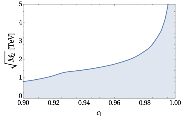
Figure 1: The upper bound on the mass of the second-lightest scalar $\sqrt{M_{2}}$ versus $\cos{\vartheta_{1}}$ in the SM2S.

In figure 2 we display the predictions for $g_{3}$ and $g_{4}$.

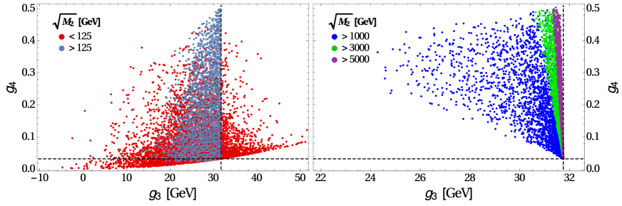
Figure 2: Scatter plots of the four-Higgs coupling $g_{4}$ versus the three-Higgs coupling $g_{3}$ in the SM2S. This figure was produced by randomly generating $\sqrt{M_{2}},\,\sqrt{M_{3}},\,w_{1},\,w_{2}\in\left[0\,\mathrm{TeV},\ 10\,\mathrm{TeV}\right]$. The dashed lines mark the values of $g_{3}$ and $g_{4}$ in the SM. The left panel includes both red points with $M_{2}<M_{1}$ and grey points with $M_{2}>M_{1}$; the right panel depicts points that have $\sqrt{M_{2}}$ larger than either 1, 3, or 5 TeV. (In order not to overcrowd the left panel, we have used in it just a subset of the set of large-$M_{2}$ points that we have generated.)

In order to produce that figure we have randomly generated $\sqrt{M_{2}}$, $\sqrt{M_{3}}$, and the VEVs $w_{1}$ and $w_{2}$ in the range 0 to 10 TeV. One sees that $g_{3}$ is always positive but below its SM value when $M_{2}>M_{1}$; when $M_{2}<M_{1}$ the allowed range for $g_{3}$ becomes much wider. When the masses of the new scalars get higher, $g_{3}$ takes values closer to the SM value. An important point is that $g_{3}$ remains of the same order of magnitude as in the SM, but $g_{4}$ may reach 15 times its SM value.

In the left panel of figure 3

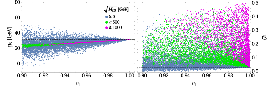
Figure 3: Scatter plots of the three-Higgs coupling $g_{3}$ (left panel) and of the four-Higgs coupling $g_{4}$ (right panel) versus $\cos{\vartheta_{1}}$ in the SM2S. The dashed lines mark the values of the couplings in the SM.

one sees that when $\cos{\vartheta_{1}}\to 1$ the coupling $g_{3}$ necessarily approaches its SM value. This behaviour is because of equation (29e) and $c_{1}>0.9$, which implies $\left|s_{1}\right|\ll c_{1}$. On the other hand, $g_{4}$ is not correlated with $\cos{\vartheta_{1}}$, as one sees in the right panel of figure 3.

3 The two-Higgs-doublet model

We next consider the model with two scalar gauge-$SU(2)$ doublets $\phi_{1}$ and $\phi_{2}$ having the same weak hypercharge. This is usually known as 2HDM. The scalar potential is given by equation (9a), where

$$V_{2} = \mu_{1}\phi_{1}^{\dagger}\phi_{1}+\mu_{2}\phi_{2}^{\dagger}\phi_{2}+\left(\mu_{3}\phi_{1}^{\dagger}\phi_{2}+\mathrm{H.c.}\right),$$ (35a)

$$V_{4} = \frac{\lambda_{1}}{2}\left(\phi_{1}^{\dagger}\phi_{1}\right)^{2}+\frac{\lambda_{2}}{2}\left(\phi_{2}^{\dagger}\phi_{2}\right)^{2}+\lambda_{3}\,\phi_{1}^{\dagger}\phi_{1}\,\phi_{2}^{\dagger}\phi_{2}+\lambda_{4}\,\phi_{1}^{\dagger}\phi_{2}\,\phi_{2}^{\dagger}\phi_{1}\hskip 19.91692pt$$ (35c)

$$+\left[\frac{\lambda_{5}}{2}\left(\phi_{1}^{\dagger}\phi_{2}\right)^{2}+\lambda_{6}\,\phi_{1}^{\dagger}\phi_{1}\,\phi_{1}^{\dagger}\phi_{2}+\lambda_{7}\,\phi_{2}^{\dagger}\phi_{2}\,\phi_{1}^{\dagger}\phi_{2}+\mathrm{H.c.}\right],$$

where $\mu_{1,2}$ and $\lambda_{1,2,3,4}$ are real. The ten (real) coefficients in $V_{4}$ may be grouped as [26]

$$\eta_{00} = \lambda_{1}+\lambda_{2}+2\lambda_{3},$$ (36a)

$$\eta=\left(\begin{array}[]{c}\eta_{1}\\ \eta_{2}\\ \eta_{3}\end{array}\right) = \left(\begin{array}[]{c}2\,\Re{\left(\lambda_{6}+\lambda_{7}\right)}\\ -2\,\Im{\left(\lambda_{6}+\lambda_{7}\right)}\\ \lambda_{1}-\lambda_{2}\end{array}\right),$$ (36h)

$$E=\left(\begin{array}[]{ccc}\eta_{11}&\eta_{12}&\eta_{13}\\ \eta_{12}&\eta_{22}&\eta_{23}\\ \eta_{13}&\eta_{23}&\eta_{33}\end{array}\right) = \left(\begin{array}[]{ccc}2\lambda_{4}+2\,\Re{\lambda_{5}}&-2\,\Im{\lambda_{5}}&2\,\Re{\left(\lambda_{6}-\lambda_{7}\right)}\\ -2\,\Im{\lambda_{5}}&2\lambda_{4}-2\,\Re{\lambda_{5}}&-2\,\Im{\left(\lambda_{6}-\lambda_{7}\right)}\\ 2\,\Re{\left(\lambda_{6}-\lambda_{7}\right)}&-2\,\Im{\left(\lambda_{6}-\lambda_{7}\right)}&\lambda_{1}+\lambda_{2}-2\lambda_{3}\end{array}\right).\hskip 17.07164pt$$ (36o)

Under a (unitary) change of basis of the scalar doublets, $\eta_{00}$ is invariant while

$$\eta\to O\eta,\quad E\to OEO^{T},$$ (37)

where $O$ is an $SO(3)$ matrix. Only quantities and procedures that are invariant under the transformation (37) are meaningful.

3.1 Unitarity conditions

We write

$$\phi_{1}=\left(\begin{array}[]{c}a\\ b\end{array}\right),\quad\phi_{2}=\left(\begin{array}[]{c}c\\ d\end{array}\right),\quad\phi_{1}^{\dagger}=\left(\begin{array}[]{cc}a^{\ast}&b^{\ast}\end{array}\right),\quad\phi_{2}^{\dagger}=\left(\begin{array}[]{cc}c^{\ast}&d^{\ast}\end{array}\right).$$ (38)

Then,

$$V_{4} = \lambda_{1}\left(\frac{a^{\ast}a^{\ast}aa+b^{\ast}b^{\ast}bb}{2}+a^{\ast}b^{\ast}ab\right)$$ (39k)

$$+\lambda_{2}\left(\frac{c^{\ast}c^{\ast}cc+d^{\ast}d^{\ast}dd}{2}+c^{\ast}d^{\ast}cd\right)$$

$$+\left(\lambda_{3}+\lambda_{4}\right)\left(a^{\ast}c^{\ast}ac+b^{\ast}d^{\ast}bd\right)$$

$$+\lambda_{3}\left(a^{\ast}d^{\ast}ad+b^{\ast}c^{\ast}bc\right)$$

$$+\lambda_{4}\left(a^{\ast}d^{\ast}bc+b^{\ast}c^{\ast}ad\right)$$

$$+\lambda_{5}\left(\frac{a^{\ast}a^{\ast}cc+b^{\ast}b^{\ast}dd}{2}+a^{\ast}b^{\ast}cd\right)$$

$$+\lambda_{5}^{\ast}\left(\frac{c^{\ast}c^{\ast}aa+d^{\ast}d^{\ast}bb}{2}+c^{\ast}d^{\ast}ab\right)$$

$$+\lambda_{6}\left(a^{\ast}a^{\ast}ac+b^{\ast}b^{\ast}bd+a^{\ast}b^{\ast}ad+a^{\ast}b^{\ast}bc\right)$$

$$+\lambda_{6}^{\ast}\left(a^{\ast}c^{\ast}aa+b^{\ast}d^{\ast}bb+a^{\ast}d^{\ast}ab+b^{\ast}c^{\ast}ab\right)$$

$$+\lambda_{7}\left(a^{\ast}c^{\ast}cc+b^{\ast}d^{\ast}dd+b^{\ast}c^{\ast}cd+a^{\ast}d^{\ast}cd\right)$$

$$+\lambda_{7}^{\ast}\left(c^{\ast}c^{\ast}ac+d^{\ast}d^{\ast}bd+c^{\ast}d^{\ast}bc+c^{\ast}d^{\ast}ad\right).$$

The relevant scattering channels are [22]:

1. The channel $Q=2,\ T_{3}=1$, with three states $aa$, $cc$, and $ac$.

2. The channel $Q=0,\ T_{3}=-1$, with three states $bb$, $dd$, and $bd$.

3. The channel $Q=1,\ T_{3}=0$, with four states $ab$, $cd$, $ad$, and $bc$.

4. The channel $Q=1,\ T_{3}=1$, with four states $ab^{\ast}$, $cd^{\ast}$, $ad^{\ast}$, and $cb^{\ast}$.

5. The channel $Q=0,\ T_{3}=0$, with eight states $aa^{\ast}$, $bb^{\ast}$, $cc^{\ast}$, $dd^{\ast}$, $ac^{\ast}$, $bd^{\ast}$, $ca^{\ast}$, and $db^{\ast}$.

Channel 5 produces the scattering matrix

$$\left(\begin{array}[]{cccccccc}2\lambda_{1}&\lambda_{1}&\lambda_{3}+\lambda_{4}&\lambda_{3}&2\lambda_{6}^{\ast}&\lambda_{6}^{\ast}&2\lambda_{6}&\lambda_{6}\\ \lambda_{1}&2\lambda_{1}&\lambda_{3}&\lambda_{3}+\lambda_{4}&\lambda_{6}^{\ast}&2\lambda_{6}^{\ast}&\lambda_{6}&2\lambda_{6}\\ \lambda_{3}+\lambda_{4}&\lambda_{3}&2\lambda_{2}&\lambda_{2}&2\lambda_{7}^{\ast}&\lambda_{7}^{\ast}&2\lambda_{7}&\lambda_{7}\\ \lambda_{3}&\lambda_{3}+\lambda_{4}&\lambda_{2}&2\lambda_{2}&\lambda_{7}^{\ast}&2\lambda_{7}^{\ast}&\lambda_{7}&2\lambda_{7}\\ 2\lambda_{6}&\lambda_{6}&2\lambda_{7}&\lambda_{7}&\lambda_{3}+\lambda_{4}&\lambda_{4}&2\lambda_{5}&\lambda_{5}\\ \lambda_{6}&2\lambda_{6}&\lambda_{7}&2\lambda_{7}&\lambda_{4}&\lambda_{3}+\lambda_{4}&\lambda_{5}&2\lambda_{5}\\ 2\lambda_{6}^{\ast}&\lambda_{6}^{\ast}&2\lambda_{7}^{\ast}&\lambda_{7}^{\ast}&2\lambda_{5}^{\ast}&\lambda_{5}^{\ast}&\lambda_{3}+\lambda_{4}&\lambda_{4}\\ \lambda_{6}^{\ast}&2\lambda_{6}^{\ast}&\lambda_{7}^{\ast}&2\lambda_{7}^{\ast}&\lambda_{5}^{\ast}&2\lambda_{5}^{\ast}&\lambda_{4}&\lambda_{3}+\lambda_{4}\end{array}\right).$$ (40)

A similarity transformation transforms the matrix (40) into the direct sum of two $4\times 4$ matrices

$$\mathcal{M}_{1} = \frac{1}{2}\left(\begin{array}[]{cc}\eta_{00}-2I&\eta^{T}\\ \eta&E+2I\times\mathbbm{1}_{3\times 3}\end{array}\right),$$ (41c)

$$\mathcal{M}_{2} = \frac{1}{2}\left(\begin{array}[]{cc}3\eta_{00}-2I&3\eta^{T}\\ 3\eta&3E+2I\times\mathbbm{1}_{3\times 3}\end{array}\right).$$ (41f)

Here,

$$I=\lambda_{3}-\lambda_{4}=\frac{\eta_{00}-\mathrm{tr}\,E}{4}$$ (42)

is invariant under a change of basis of the doublets. It is obvious that the eigenvalues of the matrices (41) are invariant under such a change too.

Channel (4) produces the scattering matrix

$$\left(\begin{array}[]{cccc}\lambda_{1}&\lambda_{4}&\lambda_{6}^{\ast}&\lambda_{6}\\ \lambda_{4}&\lambda_{2}&\lambda_{7}^{\ast}&\lambda_{7}\\ \lambda_{6}&\lambda_{7}&\lambda_{3}&\lambda_{5}\\ \lambda_{6}^{\ast}&\lambda_{7}^{\ast}&\lambda_{5}^{\ast}&\lambda_{3}\end{array}\right),$$ (43)

which may readily be shown to be similar to $\mathcal{M}_{1}$. Channel (3) produces the scattering matrix

$$\left(\begin{array}[]{cccc}\lambda_{1}&\lambda_{5}&\lambda_{6}&\lambda_{6}\\ \lambda_{5}^{\ast}&\lambda_{2}&\lambda_{7}^{\ast}&\lambda_{7}^{\ast}\\ \lambda_{6}^{\ast}&\lambda_{7}&\lambda_{3}&\lambda_{4}\\ \lambda_{6}^{\ast}&\lambda_{7}&\lambda_{4}&\lambda_{3}\end{array}\right).$$ (44)

The matrix (44) is similar to

$$\left(\begin{array}[]{cccc}&&&0\\ &\mathcal{M}_{3}&&0\\ &&&0\\ 0&0&0&I\end{array}\right),$$ (45)

where

$$\mathcal{M}_{3}=\left(\begin{array}[]{ccc}\lambda_{1}&\lambda_{5}&\sqrt{2}\lambda_{6}\\ \lambda_{5}^{\ast}&\lambda_{2}&\sqrt{2}\lambda_{7}^{\ast}\\ \sqrt{2}\lambda_{6}^{\ast}&\sqrt{2}\lambda_{7}&\lambda_{3}+\lambda_{4}\end{array}\right).$$ (46)

Channels (1) and (2) also lead to the matrix $\mathcal{M}_{3}$. Direct computation demonstrates that the eigenvalues of $\mathcal{M}_{3}$ are invariant under the transformation (37).

Thus, the unitarity conditions for the scalar potential of the 2HDM are the following: the eigenvalues of the two $4\times 4$ matrices (41) and of the $3\times 3$ matrix (46), and $I$ in equation (42), should have moduli smaller than $4\pi$. These conditions were first derived in ref. [27]. We emphasize that they are, as they should, invariant under a change of basis of the two doublets.

3.1.1 The case $\lambda_{6}=\lambda_{7}=0$

If $\lambda_{6}=\lambda_{7}=0$, then $\eta_{1}=\eta_{2}=\eta_{13}=\eta_{23}=0$ and this simplifies things considerably. The unitarity conditions are then

$$\left|\lambda_{3}+\lambda_{4}\right| < 4\pi,$$ (47a)

$$\left|\lambda_{3}-\lambda_{4}\right| < 4\pi,$$ (47b)

$$\left|\lambda_{3}+\left|\lambda_{5}\right|\right| < 4\pi,$$ (47c)

$$\left|\lambda_{3}-\left|\lambda_{5}\right|\right| < 4\pi,$$ (47d)

$$a_{+}\equiv\left|\lambda_{3}+2\lambda_{4}+3\left|\lambda_{5}\right|\right| < 4\pi,$$ (47e)

$$a_{-}\equiv\left|\lambda_{3}+2\lambda_{4}-3\left|\lambda_{5}\right|\right| < 4\pi,$$ (47f)

$$\left|\lambda_{1}+\lambda_{2}+\sqrt{\left(\lambda_{1}-\lambda_{2}\right)^{2}+4\left|\lambda_{5}\right|^{2}}\right| < 8\pi,$$ (47g)

$$\left|\lambda_{1}+\lambda_{2}-\sqrt{\left(\lambda_{1}-\lambda_{2}\right)^{2}+4\left|\lambda_{5}\right|^{2}}\right| < 8\pi,$$ (47h)

$$\left|\lambda_{1}+\lambda_{2}+\sqrt{\left(\lambda_{1}-\lambda_{2}\right)^{2}+4\lambda_{4}^{2}}\right| < 8\pi,$$ (47i)

$$\left|\lambda_{1}+\lambda_{2}-\sqrt{\left(\lambda_{1}-\lambda_{2}\right)^{2}+4\lambda_{4}^{2}}\right| < 8\pi,$$ (47j)

$$b_{+}\equiv\left|3\lambda_{1}+3\lambda_{2}+\sqrt{9\left(\lambda_{1}-\lambda_{2}\right)^{2}+4\left(2\lambda_{3}+\lambda_{4}\right)^{2}}\right| < 8\pi,$$ (47k)

$$b_{-}\equiv\left|3\lambda_{1}+3\lambda_{2}-\sqrt{9\left(\lambda_{1}-\lambda_{2}\right)^{2}+4\left(2\lambda_{3}+\lambda_{4}\right)^{2}}\right| < 8\pi.$$ (47l)

3.1.2 The case $\lambda_{1}=\lambda_{2}=\lambda_{3}=\lambda_{4}=\lambda_{5}=0$

The case $\lambda_{1}=\lambda_{2}=\lambda_{3}=\lambda_{4}=\lambda_{5}=0$ is not realistic because it produces a potential unbounded from below. Still, one may compute the unitarity conditions in that case and one obtains

$$\sqrt{\left|\lambda_{6}\right|^{2}+\left|\lambda_{7}\right|^{2}} < 2\sqrt{2}\pi,$$ (48a)

$$\sqrt{\left|\lambda_{6}\right|^{2}+\left|\lambda_{7}\right|^{2}+\left|\lambda_{6}^{2}+\lambda_{7}^{2}\right|} < \frac{4\pi}{3}.$$ (48b)

3.1.3 Consequences

We have numerically analyzed the unitarity conditions by giving random values to $\lambda_{1}$, $\lambda_{2}$, $\lambda_{3}$, $\lambda_{4}$, $\left|\lambda_{5}\right|$, $\left|\lambda_{6}\right|$, $\left|\lambda_{7}\right|$, $\arg{\left(\lambda_{5}^{\ast}\lambda_{6}\lambda_{7}\right)}$, and $\arg{\left(\lambda_{6}^{\ast}\lambda_{7}\right)}$ and then checking whether all the unitarity conditions are met. We present in figures 4–6 scatter plots with more than 8,000 allowed points each.

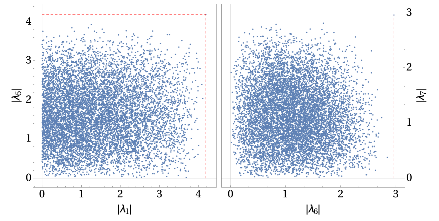
Figure 4: Scatter plots of $\left|\lambda_{1}\right|$ versus $\left|\lambda_{5}\right|$ and of $\left|\lambda_{6}\right|$ versus $\left|\lambda_{7}\right|$ with the unitarity conditions enforced. The dashed red lines indicate the bounds $\left|\lambda_{1,5}\right|<4\pi/3$ and $\left|\lambda_{6,7}\right|<2\sqrt{2}\pi/3$, respectively.

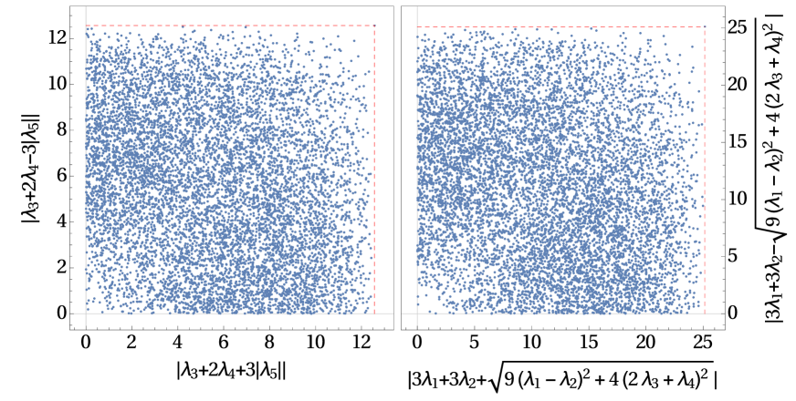
Figure 5: Scatter plots of $a_{\pm}$ and $b_{\pm}$—see equations (47e), (47f), (47k), and (47l)—with the unitarity conditions enforced. The red dashed lines indicate the bounds $a_{\pm}<4\pi$ in the left plot and $b_{\pm}<8\pi$ in the right plot.

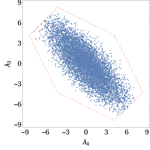
Figure 6: Scatter plots of $\lambda_{3}$ versus $\lambda_{4}$ with the unitarity conditions enforced. The dashed red lines are given by the equations $\left|\lambda_{3}-\lambda_{4}\right|=4\pi$, $\left|2\lambda_{3}+\lambda_{4}\right|=4\pi$, and $\left|\lambda_{3}+2\lambda_{4}\right|=4\pi$.

We have found that all the conditions (47) still hold even when $\lambda_{6}=\lambda_{7}=0$ is not true; also, the conditions (48) still hold even when $\lambda_{1}=\lambda_{2}=\lambda_{3}=\lambda_{4}=\lambda_{5}=0$ does not apply. In particular, the upper bounds (47b), (47e), (47f), (47k), and (47l) are sometimes attained, as illustrated in figures 6 and 5, respectively. For the individual parameters, the bounds

$$\left|\lambda_{1,2}\right| < \frac{4\pi}{3},$$ (49a)

$$\left|\lambda_{5}\right| < \frac{4\pi}{3},$$ (49b)

$$\left|\lambda_{6,7}\right| < \frac{2\sqrt{2}\pi}{3}$$ (49c)

hold and are illustrated in figure 4; the bound (49a) is suggested by inequality (47k) when $\lambda_{3}$, $\lambda_{4}$, and either $\lambda_{1}$ or $\lambda_{2}$ vanish; the bound (49b) is suggested by inequality (47e) when $\lambda_{3}=\lambda_{4}=0$, and the bound (49c) is suggested by inequality (48b) when either $\lambda_{6}$ or $\lambda_{7}$ vanishes. Finally, $\left(\lambda_{3},\,\lambda_{4}\right)$ is always within the hexagon with sides $\left|\lambda_{3}-\lambda_{4}\right|=4\pi$, $\left|2\lambda_{3}+\lambda_{4}\right|=4\pi$, and $\left|\lambda_{3}+2\lambda_{4}\right|=4\pi$, as illustrated in figure 6.

3.2 Bounded-from-below conditions

Necessary and sufficient conditions for the scalar potential of the 2HDM to be BFB were first derived in ref. [26]. Ivanov [28] and Silva [29] later produced other, equivalent conditions to the same effect. We have implemented numerically both the conditions of ref. [26] and those of ref. [29]. We have found that the Ivanov–Silva algorithm runs several times faster than the one of ref. [26]. We have also checked that all the points produced by either algorithm were validated by the other one.

The points in our scatter plots were produced by using the algorithm of ref. [29]. That algorithm runs as follows. One constructs the $4\times 4$ matrix

$$\Lambda_{E}=\left(\begin{array}[]{cc}\eta_{00}&\eta^{T}\\ -\eta&-E\end{array}\right)$$ (50)

and one computes its four eigenvalues. Then the potential is BFB if all the following conditions apply:

• All four eigenvalues are real.

• All four eigenvalues are different from each other.

• Call $\Lambda_{0}$ the largest eigenvalue. Call the other three eigenvalues $\Lambda_{1,2,3}$. The eigenvalue $\Lambda_{0}$ is positive; thus,

  $$\Lambda_{0}>\Lambda_{1,2,3},\quad\Lambda_{0}>0.$$ (51)

  (Each of $\Lambda_{1}$, $\Lambda_{2}$, and $\Lambda_{3}$ may be either positive or negative.)

• $$\frac{\left[\left(\Lambda_{E}-\Lambda_{1}\times\mathbbm{1}_{4\times 4}\right)\times\left(\Lambda_{E}-\Lambda_{2}\times\mathbbm{1}_{4\times 4}\right)\times\left(\Lambda_{E}-\Lambda_{3}\times\mathbbm{1}_{4\times 4}\right)\right]_{11}}{\left(\Lambda_{0}-\Lambda_{1}\right)\left(\Lambda_{0}-\Lambda_{2}\right)\left(\Lambda_{0}-\Lambda_{3}\right)}>0.$$ (52)

It is possible to derive analytically some necessary conditions for boundedness-from-below. Let us parameterize

$$\phi_{1}^{\dagger}\phi_{1}=r^{2}\sin^{2}{\theta},\quad\phi_{2}^{\dagger}\phi_{2}=r^{2}\cos^{2}{\theta},\quad\phi_{1}^{\dagger}\phi_{2}=e^{i\alpha}r^{2}h\sin{\theta}\cos{\theta},$$ (53)

where $0\leq\theta\leq\pi/2$ without loss of generality. Since, in the notation of equations (38),

$$r^{4}\left(1-h^{2}\right)\sin^{2}{\theta}\cos^{2}{\theta}=\phi_{1}^{\dagger}\phi_{1}\,\phi_{2}^{\dagger}\phi_{2}-\phi_{1}^{\dagger}\phi_{2}\,\phi_{2}^{\dagger}\phi_{1}=\left|ad-bc\right|^{2}\geq 0,$$ (54)

one concludes that $h^{2}\leq 1$. Thus, without loss of generality $0\leq h\leq 1$ while the phase $\alpha$ is arbitrary. Boundedness from below of $V_{4}$ means that

$$\frac{\lambda_{1}}{2}\sin^{4}{\theta}+\frac{\lambda_{2}}{2}\cos^{4}{\theta}+\left[\lambda_{3}+\lambda_{4}h^{2}+\Re{\left(\lambda_{5}e^{2i\alpha}\right)}h^{2}\right]\sin^{2}{\theta}\cos^{2}{\theta}$$ (55a)

$$+2h\,\Re{\left(\lambda_{6}e^{i\alpha}\right)}\sin^{3}{\theta}\cos{\theta}+2h\,\Re{\left(\lambda_{7}e^{i\alpha}\right)}\sin{\theta}\cos^{3}{\theta} > 0$$ (55b)

for any $\theta$, $h$, and $\alpha$. From the cases $\theta=0$ and $\theta=\pi/2$ one derives

$$\lambda_{1}>0,\quad\lambda_{2}>0.$$ (56)

Making $\alpha\to\pi+\alpha$ in inequality (55), one concludes that

$$2h\sin{\theta}\cos{\theta}\left|\Re{\left[\left(\lambda_{6}\sin^{2}{\theta}+\lambda_{7}\cos^{2}{\theta}\right)e^{i\alpha}\right]}\right| < \frac{\lambda_{1}}{2}\sin^{4}{\theta}+\frac{\lambda_{2}}{2}\cos^{4}{\theta}$$ (57c)

$$+\left[\lambda_{3}+\lambda_{4}h^{2}\right.$$

$$\left.+\Re{\left(\lambda_{5}e^{2i\alpha}\right)}h^{2}\right]\sin^{2}{\theta}\cos^{2}{\theta}.$$

Therefore, the quantity in the right-hand side of inequality (57) must be positive for any $\theta$, $h$, and $\alpha$. It is easy to see that

$$\varrho\sin^{4}{\theta}+\varsigma\cos^{4}{\theta}+\varepsilon\sin^{2}{\theta}\cos^{2}{\theta}>0\ \,\forall\theta\in\left[0,\ \frac{\pi}{2}\right]\quad\Leftrightarrow\quad\varrho>0,\ \varsigma>0,\ \varepsilon>-2\sqrt{\varrho\varsigma}.$$ (58)

Applying the statement (58) to the case $\varrho=\lambda_{1}/2$, $\varsigma=\lambda_{2}/2$, $\varepsilon=\lambda_{3}+\lambda_{4}h^{2}+\Re{\left(\lambda_{5}e^{2i\alpha}\right)}h^{2}$ for any $h\in\left[0,\ 1\right]$ and $\alpha$, one concludes that

$$\lambda_{3}>-\sqrt{\lambda_{1}\lambda_{2}},\quad\lambda_{3}+\lambda_{4}-\left|\lambda_{5}\right|>-\sqrt{\lambda_{1}\lambda_{2}}.$$ (59)

Inequalities (56) and (59) are necessary and sufficient conditions for boundedness-from-below when $\lambda_{6}=\lambda_{7}=0$ [30]; they are necessary conditions when $\lambda_{6}$ and $\lambda_{7}$ are nonzero.

We may now return to inequality (57), which implies, in principle, many more necessary conditions for boundedness-from-below. Setting for instance $\sin{\theta}=\cos{\theta}$ one concludes that

$$2h\left|\Re{\left[\left(\lambda_{6}+\lambda_{7}\right)e^{i\alpha}\right]}\right|<\frac{\lambda_{1}+\lambda_{2}}{2}+\lambda_{3}+\lambda_{4}h^{2}+\Re{\left(\lambda_{5}e^{2i\alpha}\right)}h^{2},$$ (60)

which must hold for any $h$ and $\alpha$. Therefore [31],

$$2\left|\lambda_{6}+\lambda_{7}\right|<\frac{\lambda_{1}+\lambda_{2}}{2}+\lambda_{3}+\lambda_{4}+\left|\lambda_{5}\right|.$$ (61)

We have numerically analyzed the BFB conditions by giving random values to $\lambda_{1}$, $\lambda_{2}$, $\lambda_{3}$, $\lambda_{4}$, $\left|\lambda_{5}\right|$, $\left|\lambda_{6}\right|$, $\left|\lambda_{7}\right|$, $\arg{\left(\lambda_{5}^{\ast}\lambda_{6}\lambda_{7}\right)}$, and $\arg{\left(\lambda_{6}^{\ast}\lambda_{7}\right)}$ and then checking whether the BFB conditions are met. We have confirmed that the conditions (56), (59), and (61) always hold.

3.3 Procedure

We consider the most general 2HDM and purport to find out its ranges for $g_{3}$ and $g_{4}$. We use the Higgs basis for the scalar doublets; in that basis only $\phi_{1}^{0}$ has VEV and therefore $\phi_{1}$ has the expression (2), while

$$\phi_{2}=\left(\begin{array}[]{c}C^{+}\\ \left(\sigma_{1}+i\sigma_{2}\right)\left/\sqrt{2}\right.\end{array}\right).$$ (62)

In equation (62), $\sigma_{1}$ and $\sigma_{2}$ are real fields and $C^{+}$ is the physical charged scalar of the 2HDM. We emphasize that using the Higgs basis represents no lack of generality, because both the unitarity and the BFB conditions are the same in any basis.

Since only $\phi_{1}$ has VEV, the vacuum stability conditions are $\mu_{1}=-\lambda_{1}v^{2}$ and $\mu_{3}=-\lambda_{6}v^{2}$ [33]. The coupling $\mu_{2}$ in equation (35a) is unrelated to the parameters of $V_{4}$; one may trade it for the charged-Higgs squared mass $M_{C}=\mu_{2}+\lambda_{3}v^{2}$. The mass terms of $H$, $\sigma_{1}$, and $\sigma_{2}$ are given by line (23j), with [33]

$$M=\left(\begin{array}[]{ccc}2\lambda_{1}v^{2}&2v^{2}\,\Re{\lambda_{6}}&-2v^{2}\,\Im{\lambda_{6}}\\ 2v^{2}\,\Re{\lambda_{6}}&M_{C}+\left(\lambda_{4}+\Re{\lambda_{5}}\right)v^{2}&-v^{2}\,\Im{\lambda_{5}}\\ -2v^{2}\,\Im{\lambda_{6}}&-v^{2}\,\Im{\lambda_{5}}&M_{C}+\left(\lambda_{4}-\Re{\lambda_{5}}\right)v^{2}\end{array}\right).$$ (63)

The matrix $M$ is diagonalized through equations (25)–(27).

The three invariants of $M$ are

$$I_{1}(M) = 2M_{C}+2\left(\lambda_{1}+\lambda_{4}\right)v^{2},$$ (64a)

$$I_{2}(M) = M_{C}^{2}+2\left(2\lambda_{1}+\lambda_{4}\right)v^{2}M_{C}+\left(4\lambda_{1}\lambda_{4}+\lambda_{4}^{2}-\left|\lambda_{5}\right|^{2}-4\left|\lambda_{6}\right|^{2}\right)v^{4},$$ (64b)

$$I_{3}(M) = 2\lambda_{1}v^{2}M_{C}^{2}+4\left(\lambda_{1}\lambda_{4}-\left|\lambda_{6}\right|^{2}\right)v^{4}M_{C}$$ (64c)

$$+2\left[\lambda_{1}\lambda_{4}^{2}-\lambda_{1}\left|\lambda_{5}\right|^{2}-2\lambda_{4}\left|\lambda_{6}\right|^{2}+2\,\Re{\left(\lambda_{5}^{\ast}\lambda_{6}^{2}\right)}\right]v^{6}.$$

We input parameters $\lambda_{1,2,\cdots,7}$ that satisfy both the unitarity conditions and the BFB conditions of subsections 3.1 and 3.2, respectively. We also use the values of $M_{1}$ and $v$ in equations (6). The two equations

$$M_{1}^{3}-M_{1}^{2}I_{1}(M)+M_{1}I_{2}(M)-I_{3}(M) = 0,$$ (65a)

$$\left[M_{1}^{2}I_{1}(M)-2M_{1}I_{2}(M)+3I_{3}(M)\right]\cos^{2}{\vartheta_{1}}$$

$$+M_{11}\left[M_{1}I_{1}(M)-M_{1}^{2}\right]-\left(M^{2}\right)_{11}M_{1}-I_{3}(M) = 0$$ (65b)

are quadratic in $M_{C}$. By affirming the fact that both quadratic equations (65) must hold for the same value of $M_{C}$, one is able to compute both $M_{C}$ and $\cos^{2}{\vartheta_{1}}$. We thus get to know the full matrix $M$, hence its eigenvalues $M_{2}$ and $M_{3}$ and its diagonalizing matrix $R$.

We require $\cos{\vartheta_{1}}>0.9$. We also compute the oblique parameter

$$T = \frac{1}{16\pi s_{w}^{2}m_{W}^{2}}\left[s_{1}^{2}F\left(M_{C},M_{1}\right)+\left(1-s_{1}^{2}c_{2}^{2}\right)F\left(M_{C},M_{2}\right)+\left(1-s_{1}^{2}s_{2}^{2}\right)F\left(M_{C},M_{3}\right)\right.\hskip 19.91692pt$$ (66b)

$$\left.-c_{1}^{2}F\left(M_{2},M_{3}\right)-s_{1}^{2}c_{2}^{2}F\left(M_{1},M_{3}\right)-s_{1}^{2}s_{2}^{2}F\left(M_{1},M_{2}\right)\right]+T_{\mathrm{singlets}},$$

where $T_{\mathrm{singlets}}$ is given by equation (31). We require $-0.04<T<0.20$.

We have applied the method devised in ref. [29] to guarantee that our assumed vacuum state is indeed the state with the lowest possible value of the potential. The method may be described as follows. Let the matrix $\Lambda_{E}$ in equation (50) have four eigenvalues $\Lambda_{0,1,2,3}$. We already know from the BFB conditions that those eigenvalues must be real and different from each other; let us order them as $\Lambda_{0}>\Lambda_{1}>\Lambda_{2}>\Lambda_{3}$. Let the charged-Higgs squared mass be $M_{C}$; define $\zeta\equiv 2M_{C}\left/v^{2}\right.$. Then, the assumed vacuum state is the global minimum of the potential if either $\zeta>\Lambda_{0}$, or $\Lambda_{0}>\zeta>\Lambda_{1}$, or $\Lambda_{2}>\zeta>\Lambda_{3}$. This test led us to discard about 10% of our previous set of points.

The four-Higgs vertex is given by

$$g_{4} = \frac{\lambda_{1}c_{1}^{4}}{8}+\frac{\lambda_{2}s_{1}^{4}}{8}+\frac{\left(\lambda_{3}+\lambda_{4}\right)c_{1}^{2}s_{1}^{2}}{4}+\frac{s_{1}^{2}c_{1}^{2}\left(c_{3}^{2}-s_{3}^{2}\right)\Re{\lambda_{5}}}{4}-\frac{s_{1}^{2}c_{1}^{2}c_{3}s_{3}\,\Im{\lambda_{5}}}{2}$$ (67b)

$$+\frac{s_{1}c_{1}^{3}\left(c_{3}\,\Re{\lambda_{6}}-s_{3}\,\Im{\lambda_{6}}\right)}{2}+\frac{s_{1}^{3}c_{1}\left(c_{3}\,\Re{\lambda_{7}}-s_{3}\,\Im{\lambda_{7}}\right)}{2}.$$

The three-Higgs vertex is given by

$$g_{3} = \frac{v}{\sqrt{2}}\left[\lambda_{1}c_{1}^{3}+\left(\lambda_{3}+\lambda_{4}\right)s_{1}^{2}c_{1}+s_{1}^{2}c_{1}\left(c_{3}^{2}-s_{3}^{2}\right)\Re{\lambda_{5}}-2s_{1}^{2}c_{1}c_{3}s_{3}\,\Im{\lambda_{5}}\right.$$ (68b)

$$\left.+3s_{1}c_{1}^{2}\left(c_{3}\,\Re{\lambda_{6}}-s_{3}\,\Im{\lambda_{6}}\right)+s_{1}^{3}\left(c_{3}\,\Re{\lambda_{7}}-s_{3}\,\Im{\lambda_{7}}\right)\right].$$

We also want to consider the $h_{1}C^{+}C^{-}$ vertex, which may be relevant in the discovery of the charged scalar. That vertex is given by

$$V_{4}=\cdots+h_{1}C^{+}C^{-}g_{1CC},$$ (69)

where, in the 2HDM,

$$g_{1CC}=\sqrt{2}v\left(c_{1}\lambda_{3}+s_{1}c_{3}\,\Re{\lambda_{7}}-s_{1}s_{3}\,\Im{\lambda_{7}}\right).$$ (70)

3.4 Results

As we know from subsections 3.1 and 3.2, in general $\lambda_{1}$ can take any value in between $0$ and $4\pi/3$. Once the constraint $\cos{\vartheta_{1}}>0.9$ is imposed, however, $\lambda_{1}$ can be no larger than $\sim 1$; this is illustrated in figure 7.

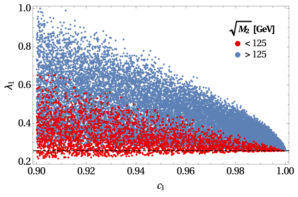
Figure 7: Scatter plots of $\lambda_{1}$ versus $\cos{\vartheta_{1}}$ in the 2HDM. The dashed line marks the value of $\lambda_{1}$ in the SM. The red points have $M_{2}<M_{1}$.

The closer $\cos{\vartheta_{1}}$ is to 1, the closer $\lambda_{1}$ must be to its SM value $M_{1}\left/\left(2v^{2}\right)\right.=0.258$; note that $\lambda_{1}$ is almost always larger than its SM value when $\cos{\vartheta_{1}}>0.9$; the minimum value that we have obtained for $\lambda_{1}$ is 0.2135.

If $\cos{\vartheta_{1}}\lesssim 0.99$, then the masses of the new scalar particles of the 2HDM, namely $\sqrt{M_{C}}$, $\sqrt{M_{2}}$, and $\sqrt{M_{3}}$ can be no larger than $\sim 700$ GeV; if $\cos{\vartheta_{1}}\lesssim 0.95$, they can be no larger than $\sim 550$ GeV. When $\cos{\vartheta_{1}}$ becomes close to 1, the masses of the new scalar particles may reach O(TeV); this is illustrated in figure 8.

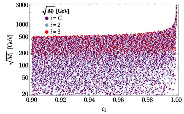
Figure 8: Scatter plots of the masses of the extra scalars of the 2HDM versus $\cos{\vartheta_{1}}$.

One sees in figure 9 that $\sqrt{M_{C}}$ and $\sqrt{M_{2}}$ differ by at most $\sim$100 GeV unless $200\,\mathrm{GeV}<\sqrt{M_{C}}<500\,\mathrm{GeV}$.

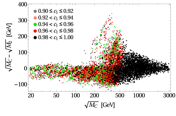
Figure 9: The difference between the mass of the charged scalar and the mass of the lightest non-SM neutral scalar versus the mass of the charged scalar in the 2HDM.

(Remember that by convention $M_{2}$ is always smaller than $M_{3}$, but they may be smaller than $M_{1}$.)

We now come to the predictions for $g_{3}$ and $g_{4}$ in the 2HDM, which are depicted in figure 10.

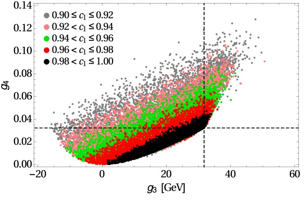
Figure 10: Scatter plot of the four-Higgs coupling $g_{4}$ versus the three-Higgs coupling $g_{3}$ in the 2HDM, for various values of $c_{1}$. The dashed lines mark the values of both couplings in the SM.

One sees that $g_{3}$ in the 2HDM has a range only slightly larger than in the SM2S, while $g_{4}$ in the 2HDM is much more restricted than in the SM2S; $g_{4}\left/g_{4}^{\mathrm{SM}}\right.\lesssim 4$ in the 2HDM but $g_{4}\left/g_{4}^{\mathrm{SM}}\right.\lesssim 15$ in the SM2S. An interesting feature is that $g_{3}$ may be zero or even negative, i.e. it may have sign opposite to the one in the SM. (We recall that the sign of $g_{3}$ is measured relative to the sign of $c_{1}$; we arrange that $c_{1}$ is always positive.) On the other hand, $g_{4}$ is always positive because of the boundedness from below of the potential.

In figure 11 we depict the coupling $g_{1CC}$ of the 125 GeV neutral scalar to a pair of charged scalars in the 2HDM. One sees that that coupling is in between -200 GeV and 1,700 GeV. The expression for $g_{1CC}$ in equation (70) is strongly dominated by the first term in the right-hand side because $c_{1}\gg s_{1}$. The preference for positive values of $g_{1CC}$ observed in figure 11 occurs because $-2\lesssim\lambda_{3}\lesssim 7$ in the 2HDM with the constraint $c_{1}>0.9$ enforced.

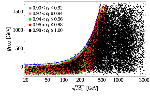
Figure 11: Scatter plot of the $h_{1}C^{+}C^{-}$ coupling $g_{1CC}$ versus the mass of the charged scalars $C^{\pm}$ in the 2HDM. The blue line with equation $g_{1CC}\!\left/\mathrm{GeV}\right.=48.5+0.54\left(\sqrt{M_{C}}\!\left/\mathrm{GeV}\right.\right)+0.0063\left(M_{C}\!\left/\mathrm{GeV}^{2}\right.\right)$ marks the approximate boundary of the allowed region.

4 The two-Higgs-doublet model plus one singlet

We consider in this section the two-Higgs-doublet model with the addition of one real $SU(2)\times U(1)$-invariant scalar field $S$. We assume a symmetry $S\to-S$. As a shorthand, we shall dub this model the 2HDM1S (other authors use just 2HDMS [34]). The quartic part of the scalar potential is

$$V_{4} = \frac{\lambda_{1}}{2}\left(\phi_{1}^{\dagger}\phi_{1}\right)^{2}+\frac{\lambda_{2}}{2}\left(\phi_{2}^{\dagger}\phi_{2}\right)^{2}+\lambda_{3}\,\phi_{1}^{\dagger}\phi_{1}\,\phi_{2}^{\dagger}\phi_{2}+\lambda_{4}\,\phi_{1}^{\dagger}\phi_{2}\,\phi_{2}^{\dagger}\phi_{1}\hskip 19.91692pt$$ (71d)

$$+\left[\frac{\lambda_{5}}{2}\left(\phi_{1}^{\dagger}\phi_{2}\right)^{2}+\lambda_{6}\,\phi_{1}^{\dagger}\phi_{1}\,\phi_{1}^{\dagger}\phi_{2}+\lambda_{7}\,\phi_{2}^{\dagger}\phi_{2}\,\phi_{1}^{\dagger}\phi_{2}+\mathrm{H.c.}\right]$$

$$+\frac{\psi}{2}\,S^{4}$$

$$+S^{2}\left(\xi_{1}\,\phi_{1}^{\dagger}\phi_{1}+\xi_{2}\,\phi_{2}^{\dagger}\phi_{2}+\xi_{3}\,\phi_{1}^{\dagger}\phi_{2}+\xi_{3}^{\ast}\,\phi_{2}^{\dagger}\phi_{1}\right).$$

4.1 Bounded-from-below conditions

Deriving necessary and sufficient BFB conditions for even a rather simple potential like the one in equation (71) is a notoriously difficult problem [35]. If $V_{4}$ were negative for some possible values of $S^{2}$, $\phi_{1}^{\dagger}\phi_{1}$, $\phi_{2}^{\dagger}\phi_{2}$, and $\phi_{1}^{\dagger}\phi_{2}$, then $V_{4}$ would tend to $-\infty$ upon multiplication of those four values by an ever-larger positive constant. Therefore, we want $V_{4}$ to be positive for all possible values of $S^{2}$, $\phi_{1}^{\dagger}\phi_{1}$, $\phi_{2}^{\dagger}\phi_{2}$, and $\phi_{1}^{\dagger}\phi_{2}$. In order to guarantee this, we proceed in the following fashion.

Necessary condition 1:

When $S^{2}=0$, equation (71) reduces to its first two lines, i.e. to the quartic potential of the 2HDM. Therefore, one must require the fulfilment of the conditions of subsection 3.2, viz. the four conditions in between equations (50) and (52).

Necessary condition 2:

When $\phi_{1}^{\dagger}\phi_{2}=0$,

$$V_{4}=\frac{1}{2}\left(\begin{array}[]{ccc}\phi_{1}^{\dagger}\phi_{1}&\phi_{2}^{\dagger}\phi_{2}&S^{2}\end{array}\right)\left(\begin{array}[]{ccc}\lambda_{1}&\lambda_{3}&\xi_{1}\\ \lambda_{3}&\lambda_{2}&\xi_{2}\\ \xi_{1}&\xi_{2}&\psi\end{array}\right)\left(\begin{array}[]{c}\phi_{1}^{\dagger}\phi_{1}\\ \phi_{2}^{\dagger}\phi_{2}\\ S^{2}\end{array}\right).$$ (72)

Since $\phi_{1}^{\dagger}\phi_{1}$, $\phi_{2}^{\dagger}\phi_{2}$, and $S^{2}$ are positive definite quantites, we must require [23, 24]

$$\psi > 0,$$ (73a)

$$\lambda_{1} > 0,$$ (73b)

$$\lambda_{2} > 0,$$ (73c)

$$A_{1}\equiv\xi_{1}+\sqrt{\lambda_{1}\psi} > 0,$$ (73d)

$$A_{2}\equiv\xi_{2}+\sqrt{\lambda_{2}\psi} > 0,$$ (73e)

$$A_{3}\equiv\lambda_{3}+\sqrt{\lambda_{1}\lambda_{2}} > 0,$$ (73f)

$$\sqrt{\lambda_{1}\lambda_{2}\psi}+\xi_{2}\sqrt{\lambda_{1}}+\xi_{1}\sqrt{\lambda_{2}}+\lambda_{3}\sqrt{\psi}+\sqrt{2A_{1}A_{2}A_{3}} > 0.$$ (73g)

After enforcing the necessary condition 1, we know that $V_{4}>0$ when only the first two lines of the potential (71) exist; after enforcing the inequality (73a), we know that $V_{4}>0$ when only the third line exists. If we guarantee that the fourth line of the potential (71) is always positive too, then we will be sure that $V_{4}$ is always positive. We therefore have the following

Sufficient condition:

If, besides the two necessary conditions,

$$\xi_{1}+\xi_{2} > 0,$$ (74a)

$$\xi_{1}\xi_{2}-\left|\xi_{3}\right|^{2} > 0,$$ (74b)

then $V_{4}$ is BFB.

Among the sets of parameters of the potential (71) that we have randomly generated, there were some that met both the two necessary conditions and the sufficient conditions (74); we have used those sets of parameters. There were many other sets that satisfied the two necessary conditions but did not meet the sufficient conditions (74); for those sets, we have numerically found the absolute minimum of $V_{4}$. We have done this by using $S^{2}=1$ together with equations (53) and by minimizing $V_{4}$ in the domain $r^{2}>0$, $0\leq\theta\leq\pi/2$, $0\leq h\leq 1$, and $0\leq\alpha<2\pi$. If the minimum of $V_{4}$ is positive, then the set of input parameters is good, else the set of input parameters is bad and one must discard it.

4.2 Unitarity conditions

There are the same five scattering channels as in the 2HDM, cf. subsection 3.1; but the channel $Q=T_{3}=0$ has an additional scattering state $S^{2}$. Additionally, there are two extra scattering channels:

• The channel $Q=1,\ T_{3}=1/2$ with the two states $aS$ and $cS$.

• The channel $Q=0,\ T_{3}=-1/2$ with the two states $bS$ and $dS$.

Both these channels produce a scattering matrix

$$\mathcal{M}_{4}=2\left(\begin{array}[]{cc}\xi_{1}&\xi_{3}\\ \xi_{3}^{\ast}&\xi_{2}\end{array}\right).$$ (75)

Channels 1 and 2 of subsection 3.1 again produce the scattering matrix (46). Channel (3) produces that matrix together with the additional eigenvalue $I$ of equation (42). Channel (2) produces the scattering matrix (41c). Finally, channel 5 has the additional scattering state $S^{2}$ and therefore, instead of producing both the matrix $\mathcal{M}_{1}$ of equation (41c) and the matrix $\mathcal{M}_{2}$ of equation (41f), it produces $\mathcal{M}_{1}$ together with

$$\mathcal{M}_{2}^{\prime}=\left(\begin{array}[]{cc}6\psi&\sqrt{2}\,\bar{\xi}^{T}\\ \sqrt{2}\,\bar{\xi}&\mathcal{M}_{2}\end{array}\right),\quad\mbox{where}\quad\bar{\xi}=\left(\begin{array}[]{c}\xi_{1}+\xi_{2}\\ 2\,\Re{\xi_{3}}\\ -2\,\Im{\xi_{3}}\\ \xi_{1}-\xi_{2}\end{array}\right).$$ (76)

Thus, the unitarity conditions for the 2HDM1S are the following: both $\left|I\right|$ and the moduli of all the eigenvalues of the $2\times 2$ matrix $\mathcal{M}_{4}$, of the $3\times 3$ matrix $\mathcal{M}_{3}$, of the $4\times 4$ matrix $\mathcal{M}_{1}$, and of the $5\times 5$ matrix $\mathcal{M}_{2}^{\prime}$ must be smaller than $4\pi$.

4.3 Procedure

Just as in the previous section, we utilize the Higgs basis for the two doublets, i.e. equations (2) and (62). We also write $S=w+\sigma$, where $w$ is the VEV of the scalar $S$ and $\sigma$ is a field. The mass terms of the scalars are

$$V=\cdots+M_{C}C^{-}C^{+}+\frac{1}{2}\left(\begin{array}[]{cccc}H&\sigma_{1}&\sigma_{2}&\sigma\end{array}\right)M\left(\begin{array}[]{c}H\\ \sigma_{1}\\ \sigma_{2}\\ \sigma\end{array}\right),$$ (77)

with

$$M=\left(\begin{array}[]{cccc}2\lambda_{1}v^{2}&2v^{2}\,\Re{\lambda_{6}}&-2v^{2}\,\Im{\lambda_{6}}&2\sqrt{2}vw\xi_{1}\\ 2v^{2}\,\Re{\lambda_{6}}&M_{C}+\left(\lambda_{4}+\Re{\lambda_{5}}\right)v^{2}&-v^{2}\,\Im{\lambda_{5}}&2\sqrt{2}vw\,\Re{\xi_{3}}\\ -2v^{2}\,\Im{\lambda_{6}}&-v^{2}\,\Im{\lambda_{5}}&M_{C}+\left(\lambda_{4}-\Re{\lambda_{5}}\right)v^{2}&-2\sqrt{2}vw\,\Im{\xi_{3}}\\ 2\sqrt{2}vw\xi_{1}&2\sqrt{2}vw\,\Re{\xi_{3}}&-2\sqrt{2}vw\,\Im{\xi_{3}}&4\psi w^{2}\end{array}\right),$$ (78)

cf. equation (63). One diagonalizes $M$ as

$$M = R^{T}\,\mathrm{diag}\left(M_{1},\,M_{2},\,M_{3},\,M_{4}\right)R,$$ (79a)

$$\left(\begin{array}[]{c}H\\ \sigma_{1}\\ \sigma_{2}\\ \sigma\end{array}\right) = R^{T}\left(\begin{array}[]{c}h_{1}\\ h_{2}\\ h_{3}\\ h_{4}\end{array}\right),$$ (79j)

where $R$ is a $4\times 4$ orthogonal matrix. The squared mass $M_{1}$ is given by equation (6a). Without loss of generality, $M_{2}<M_{3}<M_{4}$. Just as in the previous sections, we require

$$R_{11}\equiv c_{1}>0.9.$$ (80)

The expression for the oblique parameter $T$ is [25]

$$T = \frac{1}{16\pi s_{w}^{2}m_{W}^{2}}\left\{\sum_{k=1}^{4}\left[\left(R_{k2}\right)^{2}+\left(R_{k3}\right)^{2}\right]F\left(M_{C},\,M_{k}\right)\right.$$ (81d)

$$-\sum_{k=1}^{3}\,\sum_{k^{\prime}=k+1}^{4}\left(R_{k2}R_{k^{\prime}3}-R_{k^{\prime}2}R_{k3}\right)^{2}F\left(M_{k},\,M_{k^{\prime}}\right)$$

$$+3\sum_{k=2}^{4}\left(R_{k1}\right)^{2}\left[F\left(M_{k},\,m_{Z}^{2}\right)-F\left(M_{k},\,m_{W}^{2}\right)\right]$$

$$\left.+3\left(c_{1}^{2}-1\right)\left[F\left(M_{1},\,m_{Z}^{2}\right)-F\left(M_{1},\,m_{W}^{2}\right)\right]\right\},$$

and we demand $-0.04<T<0.20$.

We input random values for the 15 real parameters $M_{C}$, $\lambda_{1,2,3,4}$, $\left|\lambda_{5,6,7}\right|$, $\psi$, $\xi_{1,2}$, $\left|\xi_{3}\right|$, $\arg{\left(\lambda_{5}^{\ast}\lambda_{6}\lambda_{7}\right)}$, $\arg{\left(\lambda_{6}^{\ast}\lambda_{7}\right)}$, and $\arg{\left(\lambda_{6}^{\ast}\xi_{3}\right)}$. We moreover input $M_{1}$ and $v^{2}$ given in equations (6). Then,

1. We require the input parameters to satisfy the BFB conditions of subsection 4.1—this may imply a numerical minimization of $V_{4}$ to check that $V_{4}>0$.

2. We require the input parameters to satisfy the unitarity conditions written after equation (76).

3. We compute the VEV $w$ from the condition that $M_{1}$ should be an eigenvalue of the matrix $M$.

4. We enforce the conditions in appendix C. They guarantee that the vacuum state with $v=174$ GeV and $w\neq 0$ has a lower value of the potential than all the other possible stability points of the potential.

5. We compute the full matrix $M$, its eigenvalues $M_{2,3,4}$, and its diagonalizing matrix $R$; we choose the overall sign of $R$ such that $R_{11}\equiv c_{1}>0$.

6. We impose both the condition (80) and the condition that the oblique parameter $T$ is within its experimental bounds.

7. We compute the couplings

   $$g_{3} = \frac{v}{\sqrt{2}}\left\{\lambda_{1}c_{1}^{3}+\left(\lambda_{3}+\lambda_{4}\right)c_{1}\left[\left(R_{12}\right)^{2}+\left(R_{13}\right)^{2}\right]\right.$$ (82e)

   $$+c_{1}\left[\left(R_{12}\right)^{2}-\left(R_{13}\right)^{2}\right]\Re{\lambda_{5}}-2c_{1}R_{12}R_{13}\,\Im{\lambda_{5}}$$

   $$\left.+3c_{1}^{2}\left(R_{12}\Re{\lambda_{6}}-R_{13}\Im{\lambda_{6}}\right)+\left[\left(R_{12}\right)^{2}+\left(R_{13}\right)^{2}\right]\left(R_{12}\Re{\lambda_{7}}-R_{13}\Im{\lambda_{7}}\right)\right\}$$

   $$+2\psi w\left(R_{14}\right)^{3}+\xi_{1}c_{1}R_{14}\left(wc_{1}+\sqrt{2}vR_{14}\right)+\xi_{2}wR_{14}\left[\left(R_{12}\right)^{2}+\left(R_{13}\right)^{2}\right]\hskip 19.91692pt$$

   $$+\sqrt{2}R_{14}\left(vR_{14}+\sqrt{2}wc_{1}\right)\left(R_{12}\Re{\xi_{3}}-R_{13}\Im{\xi_{3}}\right),$$

   $$g_{4} = \frac{\lambda_{1}c_{1}^{4}}{8}+\frac{\lambda_{2}}{8}\left[\left(R_{12}\right)^{2}+\left(R_{13}\right)^{2}\right]^{2}+\frac{\lambda_{3}+\lambda_{4}}{4}\,c_{1}^{2}\left[\left(R_{12}\right)^{2}+\left(R_{13}\right)^{2}\right]$$ (83e)

   $$+\frac{\Re{\lambda_{5}}}{4}\,c_{1}^{2}\left[\left(R_{12}\right)^{2}-\left(R_{13}\right)^{2}\right]-\frac{\Im{\lambda_{5}}}{2}\,c_{1}^{2}R_{12}R_{13}$$

   $$+\frac{c_{1}^{3}}{2}\left(R_{12}\,\Re{\lambda_{6}}-R_{13}\,\Im{\lambda_{6}}\right)+\frac{c_{1}\left[\left(R_{12}\right)^{2}+\left(R_{13}\right)^{2}\right]}{2}\left(R_{12}\,\Re{\lambda_{7}}-R_{13}\,\Im{\lambda_{7}}\right)\hskip 19.91692pt$$

   $$+\frac{\psi}{2}\left(R_{14}\right)^{4}$$

   $$+\left(R_{14}\right)^{2}\left\{\frac{\xi_{1}c_{1}^{2}}{2}+\frac{\xi_{2}}{2}\left[\left(R_{12}\right)^{2}+\left(R_{13}\right)^{2}\right]+c_{1}\left(R_{12}\,\Re{\xi_{3}}-R_{13}\,\Im{\xi_{3}}\right)\right\},$$

   $$g_{1CC} = \sqrt{2}v\left(c_{1}\lambda_{3}+R_{12}\,\Re{\lambda_{7}}-R_{13}\,\Im{\lambda_{7}}\right)+2w\xi_{2}R_{14}.$$ (84)

4.4 Results

In figure 12 we have plotted the differences among the masses of the scalars against the mass of the charged scalar.

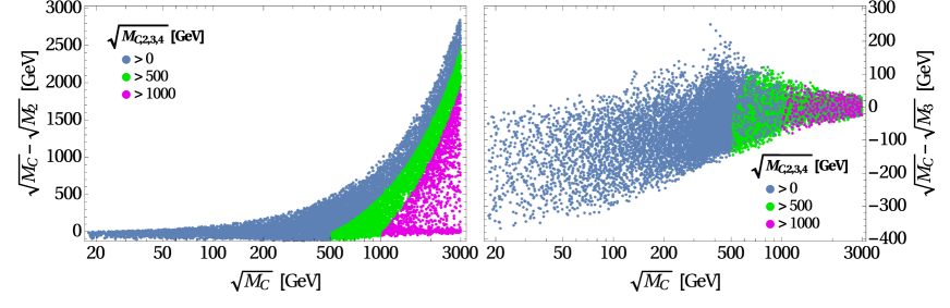
Figure 12: The differences between the masses of the two lightest non-SM neutral scalars and the mass of the charged scalar versus the mass of the charged scalar in the 2HDM1S. Green points have all the scalars with mass larger than 500 GeV; magenta points have all the scalars with mass larger than 1 TeV.

One sees that $\sqrt{M_{C}}$ and $\sqrt{M_{3}}$ cannot be more than $\sim 300$ GeV from each other, but $\sqrt{M_{2}}$ may be much smaller than both of them.

In figure 13 we present a scatter plot of the mass of the lightest non-SM neutral scalar against $c_{1}$.

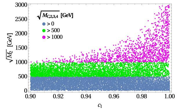
Figure 13: The mass of the lightest non-SM neutral scalar versus $R_{11}$ in the 2HDM1S. Green points have all the scalars with mass larger than 500 GeV; magenta points have all the scalars with mass larger than 1 TeV.

One sees that, contrary to what happens in the 2HDM (cf. figure 8), $\sqrt{M_{2}}$ may reach 1 TeV even when $c_{1}$ is as low as 0.9.

We depict in figure 14 the three- and four-Higgs couplings $g_{3}$ and $g_{4}$ in the 2HDM1S.

Figure 14: In the left panel, the four-Higgs coupling $g_{4}$ versus the three-Higgs coupling $g_{3}$ in the 2HDM1S for various values of $c_{1}$. The right panel contains the same points as the left panel but with different colours depending on whether $M_{2}$ is larger or smaller than $M_{1}$. The dashed lines mark the values of the couplings in the SM.

The main difference relative to the 2HDM (cf. figure 10) is that $g_{4}$ may be much higher, just as in the SM2S. In the 2HDM1S there is no clear correlation between $g_{3}$ and $g_{4}$.

In figure 15 we have plotted the $h_{1}C^{+}C^{-}$ coupling $g_{1CC}$.

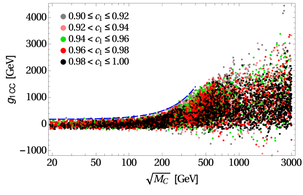
Figure 15: Scatter plot of $g_{1CC}$ versus the mass of the charged scalars $C^{\pm}$ in the 2HDM1S. The blue line with equation $g_{1CC}\!\left/\mathrm{GeV}\right.=174.9+0.138\left(\sqrt{M_{C}}\!\left/\mathrm{GeV}\right.\right)+0.0073\left(M_{C}\!\left/\mathrm{GeV}^{2}\right.\right)$ marks the approximate boundary of the allowed region when $\sqrt{M_{C}}<400$ GeV.

That coupling in the 2HDM1S may be more than two times larger than in the 2HDM; very large values of $g_{1CC}$ occur even for $c_{1}$ very close to 1. This is because the right-hand side of equation (84) may be dominated by its fourth term when $w\gg v$. The first term displays the same behaviour as the corresponding term in the 2HDM, viz. it is usually positive and no larger than 1,500 GeV, but it is often overwhelmed by the fourth term.

5 Conclusions

In this paper we have emphasized that both the bounded-from-below (BFB) conditions and the unitarity conditions for the two-Higgs-doublet model (2HDM) are invariant under a change of the basis used for the two doublets. Therefore, one may implement those conditions directly in the Higgs basis, viz. the basis where only one doublet has vacuum expectation value. This procedure allows one to extract bounds on the masses and couplings of the scalar particles of the most general 2HDM, disregarding any symmetry that a particular 2HDM may possess. We have focussed on the three couplings $g_{3}\left(h_{1}\right)^{3}$, $g_{4}\left(h_{1}\right)^{4}$, and $g_{1CC}h_{1}C^{+}C^{-}$, where $h_{1}$ is the observed neutral scalar with mass 125 GeV and $C^{\pm}$ are the charged scalars of the 2HDM.

We have utilized the same procedure for two other models, namely the Standard Model with the addition of two real singlets (SM2S) and the two-Higgs-doublet model with the addition of one real singlet (2HDM1S), in both cases with reflection symmetries acting on each of the singlets. We have found, for instance, that:

• The coupling $g_{3}$ may, in both the 2HDM and the 2HDM1S, have sign opposite to the one in the SM. On the other hand, in any of the three models that we have studied, $\left|g_{3}\right|$ can hardly be much larger than in the SM.

• The coupling $g_{4}$, which is always positive because of BFB, may for all practical purposes be equal to zero in all the three models. (As a matter of fact, $g_{3}=g_{4}=0$ is possible in all three models.) But it may also be much larger than in the SM. A distinguished feature is that $g_{4}$ may be much larger (up to $g_{4}\sim 0.5$) in the models containing singlets than in the 2HDM, wherein it can at best reach $g_{4}\sim 0.13$.

• The coupling $g_{1CC}$ may be of order TeV, but only when the mass of $C^{\pm}$ exceeds 300 GeV; in general, a positive $g_{1CC}$ may be larger for higher masses of $C^{\pm}$, but $g_{1CC}$ may also be negative for any $C^{\pm}$ mass. Moreover, $g_{1CC}$ may be more than two times larger (either positive or negative) in the 2HDM1S than in the 2HDM.

A comparison of the predictions of the three models for $g_{3}$ and $g_{4}$ is depicted in figure 16.

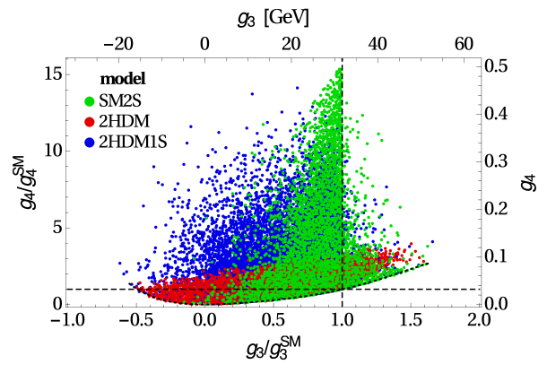
Figure 16: Scatter plot of $g_{4}\left/g_{4}^{\mathrm{SM}}\right.$ versus $g_{3}\left/g_{3}^{\mathrm{SM}}\right.$ in the three models that we have studied. The dashed lines mark the SM values $g_{3}\left/g_{3}^{\mathrm{SM}}\right.=g_{4}\left/g_{4}^{\mathrm{SM}}\right.=1$. The dotted line, with equation $g_{4}\left/g_{4}^{\mathrm{SM}}\right.=2.06\left(g_{3}\left/g_{3}^{\mathrm{SM}}\right.\right)^{2}-2.84\left(g_{3}\left/g_{3}^{\mathrm{SM}}\right.\right)^{3}+2.44\left(g_{3}\left/g_{3}^{\mathrm{SM}}\right.\right)^{4}-0.67\left(g_{3}\left/g_{3}^{\mathrm{SM}}\right.\right)^{5}$, marks the approximate boundary of the allowed region for $-0.6<g_{3}\left/g_{3}^{\mathrm{SM}}\right.<1.6$.

We emphasize that our method may be used to obtain bounds and/or correlations among other parameters and/or observables of these models. Unfortunately, it may be difficult to generalize our work to more complicated models, both because they may contain too many parameters and because it is very difficult to derive full BFB conditions for even rather simple models.

Acknowledgements: L.L. thanks Pedro Miguel Ferreira and Igor Ivanov, and D.J. thanks Artūras Acus, for useful discussions. D.J. thanks the Lithuanian Academy of Sciences for support through the project DaFi2018. The work of L.L. is supported by the Portuguese Fundação para a Ciência e a Tecnologia through the projects CERN/FIS-NUC/0010/2015, CERN/FIS-PAR/0004/2017, and UID/FIS/00777/2013; those projects are partly funded by POCTI (FEDER), COMPETE, QREN, and the European Union.

Appendix A The Higgs Singlet Model

The Higgs Singlet Model (HSM) is the Standard Model with the addition of one real scalar singlet $S$. We furthermore assume a symmetry $S\to-S$. The scalar potential

$$V=\mu\phi_{1}^{\dagger}\phi_{1}+m^{2}S^{2}+\frac{\lambda}{2}\left(\phi_{1}^{\dagger}\phi_{1}\right)^{2}+\frac{\psi}{2}\,S^{4}+\xi S^{2}\phi_{1}^{\dagger}\phi_{1}$$ (A1)

has just five parameters $\mu$, $m^{2}$, $\lambda$, $\psi$, and $\xi$. The bounded-from-below (BFB) conditions are

$$\lambda>0,\quad\psi>0,\quad\xi>-\sqrt{\lambda\psi}.$$ (A2)

The unitarity conditions are

$$\left|\lambda\right|<4\pi,\quad\left|\xi\right|<2\pi,\quad\left|3\lambda+6\psi+\sqrt{\left(3\lambda-6\psi\right)^{2}+16\xi^{2}}\right|<8\pi.$$ (A3)

We assume that $\phi_{1}$ has VEV $v$ and $S$ has VEV $w$. We write $S=w+\sigma$ together with equation (2). The mass matrix for $H$ and $\sigma$ is

$$\left(\begin{array}[]{cc}2\lambda v^{2}&2\sqrt{2}\xi vw\\ 2\sqrt{2}\xi vw&4\psi w^{2}\end{array}\right)=\left(\begin{array}[]{cc}c&-s\\ s&c\end{array}\right)\left(\begin{array}[]{cc}M_{1}&0\\ 0&M_{2}\end{array}\right)\left(\begin{array}[]{cc}c&s\\ -s&c\end{array}\right),$$ (A4)

where $c\equiv\cos{\vartheta}$ and $s\equiv\sin{\vartheta}$. We assume $|c|>0.9$. The oblique parameter

$$T=\frac{3s^{2}}{16\pi s_{w}^{2}m_{W}^{2}}\left[F\left(M_{1},m_{W}^{2}\right)-F\left(M_{1},m_{Z}^{2}\right)-F\left(M_{2},m_{W}^{2}\right)+F\left(M_{2},m_{Z}^{2}\right)\right]$$ (A5)

must satisfy $-0.04<T<0.20$. The three- and four-Higgs couplings are given by

$$\frac{g_{3}}{g_{3}^{\mathrm{SM}}} = c^{3}+\frac{\sqrt{2}v}{w}\,s^{3},$$ (A6a)

$$g_{4} = \frac{\lambda}{8}\,c^{4}+\frac{\psi}{2}\,s^{4}+\frac{\xi}{2}\,c^{2}s^{2}.$$ (A6b)

In figure 17 we compare the predictions of the HSM and of the SM2S for $g_{3}$ and $g_{4}$. One sees that there is no substantial difference between the two models.

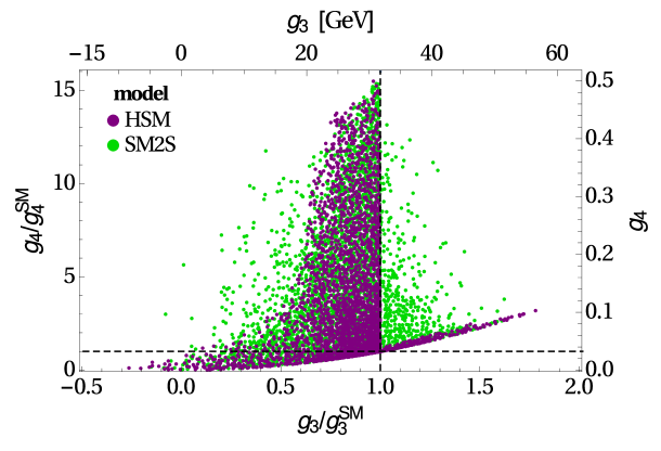
Figure 17: Scatter plot of $g_{4}\left/g_{4}^{\mathrm{SM}}\right.$ versus $g_{3}\left/g_{3}^{\mathrm{SM}}\right.$ in the HSM and in the SM2S. The dashed lines mark the Standard Model values $g_{3}\left/g_{3}^{\mathrm{SM}}\right.=g_{4}\left/g_{4}^{\mathrm{SM}}\right.=1$.

Appendix B Other stability points of the SM2S potential

In this appendix we consider more carefully the various stability points of the potential of the SM2S in equation (9). The vacuum value of that potential is given by

$$V_{0}\equiv\left\langle 0\left|V\right|0\right\rangle = \mu_{1}v^{2}+m_{1}^{2}w_{1}^{2}+m_{2}^{2}w_{2}^{2}$$ (B1c)

$$+\frac{\lambda_{1}v^{4}}{2}+\frac{\psi_{1}w_{1}^{4}}{2}+\frac{\psi_{2}w_{2}^{4}}{2}$$

$$+\psi_{3}w_{1}^{2}w_{2}^{2}+\xi_{1}v^{2}w_{1}^{2}+\xi_{2}v^{2}w_{2}^{2}.$$

Equations (22) follow from the assumption that $v$, $w_{1}$, and $w_{2}$ are not zero. Defining

$$d\equiv\lambda_{1}\psi_{1}\psi_{2}+2\psi_{3}\xi_{1}\xi_{2}-\lambda_{1}\psi_{3}^{2}-\psi_{1}\xi_{2}^{2}-\psi_{2}\xi_{1}^{2},$$ (B2)

one obtains

$$V_{0} = -\frac{\lambda_{1}v^{4}}{2}-\frac{\psi_{1}w_{1}^{4}}{2}-\frac{\psi_{2}w_{2}^{4}}{2}-\psi_{3}w_{1}^{2}w_{2}^{2}-\xi_{1}v^{2}w_{1}^{2}-\xi_{2}v^{2}w_{2}^{2}$$ (B3a)

$$= \frac{1}{2d}\left[\left(\psi_{3}^{2}-\psi_{1}\psi_{2}\right)\mu_{1}^{2}+\left(\xi_{2}^{2}-\lambda_{1}\psi_{2}\right)\left(m_{1}^{2}\right)^{2}+\left(\xi_{1}^{2}-\lambda_{1}\psi_{1}\right)\left(m_{2}^{2}\right)^{2}\right.\hskip 22.76219pt$$ (B3d)

$$+2\left(\xi_{1}\psi_{2}-\psi_{3}\xi_{2}\right)\mu_{1}m_{1}^{2}+2\left(\xi_{2}\psi_{1}-\psi_{3}\xi_{1}\right)\mu_{1}m_{2}^{2}$$

$$\left.+2\left(\lambda_{1}\psi_{3}-\xi_{1}\xi_{2}\right)m_{1}^{2}m_{2}^{2}\right].$$

The mass matrix $M$ of the scalars is real and symmetric and is given in equation (24). We assume that $M$ has three positive eigenvalues $M_{1}$, $M_{2}$, and $M_{3}$. It follows that all the principal minors of $M$ are positive. (This is called ‘Sylvester’s criterion’ [36].) Thus,

$$\lambda_{1} > 0,$$ (B4a)

$$\psi_{1} > 0,$$ (B4b)

$$\psi_{2} > 0,$$ (B4c)

$$\lambda_{1}\psi_{1}-\xi_{1}^{2} > 0,$$ (B4d)

$$\lambda_{1}\psi_{2}-\xi_{2}^{2} > 0,$$ (B4e)

$$\psi_{1}\psi_{2}-\psi_{3}^{2} > 0,$$ (B4f)

$$d > 0.$$ (B4g)

These inequalities display some resemblance to the BFB conditions (20), (21).

We now consider other stability points of the potential where either $v$ or $w_{1}$ or $w_{2}$ vanish.

1. There is a stability point where $w_{1}=w_{2}=0$. At that point the potential has the value

   $$V^{(1)}\equiv-\frac{\mu_{1}^{2}}{2\lambda_{1}}.$$ (B5)

2. Similarly, there are stability points where either $v=w_{1}=0$ or $v=w_{2}=0$. At those two points the values of the potential are, respectively,

   $$V^{(2)} \equiv -\frac{\left(m_{2}^{2}\right)^{2}}{2\psi_{2}},$$ (B6a)

   $$V^{(3)} \equiv -\frac{\left(m_{1}^{2}\right)^{2}}{2\psi_{1}}.$$ (B6b)

3. There is a stability point of the potential where $v=0$ but $w_{1}$ and $w_{2}$ are nonzero. At that point the potential takes the value

   $$V^{(4)}\equiv\frac{-\psi_{2}\left(m_{1}^{2}\right)^{2}-\psi_{1}\left(m_{2}^{2}\right)^{2}+2\psi_{3}m_{1}^{2}m_{2}^{2}}{2\left(\psi_{1}\psi_{2}-\psi_{3}^{2}\right)}.$$ (B7)

4. Similarly, there is a stability point where $w_{1}=0$ but $v\neq 0$ and $w_{2}\neq 0$. At that point the value of the potential is

   $$V^{(5)}\equiv\frac{-\psi_{2}\mu_{1}^{2}-\lambda_{1}\left(m_{2}^{2}\right)^{2}+2\xi_{2}\mu_{1}m_{2}^{2}}{2\left(\lambda_{1}\psi_{2}-\xi_{2}^{2}\right)}.$$ (B8)

5. Finally, there is another stability point with value

   $$V^{(6)}\equiv\frac{-\psi_{1}\mu_{1}^{2}-\lambda_{1}\left(m_{1}^{2}\right)^{2}+2\xi_{1}\mu_{1}m_{1}^{2}}{2\left(\lambda_{1}\psi_{1}-\xi_{1}^{2}\right)}$$ (B9)

   of the potential.

From inequalities (B4c) and (B4f) it follows that $V^{(4)}\leq V^{(2)}$ is equivalent to

$$\psi_{2}\left[-\psi_{2}\left(m_{1}^{2}\right)^{2}-\psi_{1}\left(m_{2}^{2}\right)^{2}+2\psi_{3}m_{1}^{2}m_{2}^{2}\right]\leq\left(\psi_{3}^{2}-\psi_{1}\psi_{2}\right)\left(m_{2}^{2}\right)^{2},$$ (B10)

which in turn is equivalent to

$$-\left(\psi_{2}m_{1}^{2}-\psi_{3}m_{2}^{2}\right)^{2}\leq 0,$$ (B11)

and this is obvioulsy true. One thus concludes that $V^{(4)}$ can never be larger than $V^{(2)}$. In similar fashion one finds that

$$V^{(4)} \leq V^{(2)},$$ (B12a)

$$V^{(4)} \leq V^{(3)},$$ (B12b)

$$V^{(5)} \leq V^{(1)},$$ (B12c)

$$V^{(5)} \leq V^{(2)},$$ (B12d)

$$V^{(6)} \leq V^{(1)},$$ (B12e)

$$V^{(6)} \leq V^{(3)}.$$ (B12f)

Next consider the inequality $V_{0}\leq V^{(4)}$. Because of (B4f) and (B4g), it is equivalent to

$$\left(\psi_{1}\psi_{2}-\psi_{3}^{2}\right)\left[\left(\psi_{3}^{2}-\psi_{1}\psi_{2}\right)\mu_{1}^{2}+\left(\xi_{2}^{2}-\lambda_{1}\psi_{2}\right)\left(m_{1}^{2}\right)^{2}\right.$$ (B13a)

$$+\left(\xi_{1}^{2}-\lambda_{1}\psi_{1}\right)\left(m_{2}^{2}\right)^{2}+2\left(\xi_{1}\psi_{2}-\psi_{3}\xi_{2}\right)\mu_{1}m_{1}^{2}$$ (B13b)

$$\left.+2\left(\xi_{2}\psi_{1}-\psi_{3}\xi_{1}\right)\mu_{1}m_{2}^{2}+2\left(\lambda_{1}\psi_{3}-\xi_{1}\xi_{2}\right)m_{1}^{2}m_{2}^{2}\right] \leq d\left[-\psi_{2}\left(m_{1}^{2}\right)^{2}\right.\hskip 19.91692pt$$ (B13e)

$$-\psi_{1}\left(m_{2}^{2}\right)^{2}$$

$$\left.+2\psi_{3}m_{1}^{2}m_{2}^{2}\right].$$

Introducing the expression for $d$ in equation (B2), one finds that the inequality (B13) is equivalent to

$$\left(\psi_{1}\psi_{1}-\psi_{3}^{2}\right)\left[\left(\psi_{3}^{2}-\psi_{1}\psi_{2}\right)\mu_{1}^{2}+2\left(\xi_{1}\psi_{2}-\psi_{3}\xi_{2}\right)\mu_{1}m_{1}^{2}\right.$$ (B14a)

$$\left.+2\left(\xi_{2}\psi_{1}-\psi_{3}\xi_{1}\right)\mu_{1}m_{2}^{2}\right]-\left(m_{1}^{2}\right)^{2}\left(\psi_{2}\xi_{1}-\psi_{3}\xi_{2}\right)^{2}$$ (B14b)

$$-\left(m_{2}^{2}\right)^{2}\left(\psi_{1}\xi_{2}-\psi_{3}\xi_{1}\right)^{2}-2m_{1}^{2}m_{2}^{2}\left(\psi_{2}\xi_{1}-\psi_{3}\xi_{2}\right)\left(\psi_{1}\xi_{2}-\psi_{3}\xi_{1}\right) \leq 0.$$ (B14c)

This may be written as

$$\left[\left(\psi_{3}^{2}-\psi_{1}\psi_{2}\right)\mu_{1}+\left(\psi_{2}\xi_{1}-\psi_{3}\xi_{2}\right)m_{1}^{2}+\left(\psi_{1}\xi_{2}-\psi_{3}\xi_{1}\right)m_{2}^{2}\right]^{2}\geq 0,$$ (B15)

which is of course true. In similar fashion one obtains that

$$V_{0} \leq V^{(4)},$$ (B16a)

$$V_{0} \leq V^{(5)},$$ (B16b)

$$V_{0} \leq V^{(6)}.$$ (B16c)

We have thus demonstrated that, because of our assumption that all three eigenvalues of the matrix $M$ are positive, $V_{0}$ is smaller than $V^{1,2,3,4,5,6}$, viz. the stability point of $V$ with nonzero $v$, $w_{1}$, and $w_{2}$ is the vacuum.

This result may be easily understood in the following way. The potential (9) of the SM2S may be rewritten

$$V=\frac{1}{2}\,X^{T}\Lambda X+V_{0},$$ (B17)

where $V_{0}$ is the vacuum expectation value of the potential given in equation (B3a) and

$$X=\left(\begin{array}[]{c}\phi_{1}^{\dagger}\phi_{1}-v^{2}\\ S_{1}^{2}-w_{1}^{2}\\ S_{2}^{2}-w_{2}^{2}\end{array}\right),\quad\Lambda=\left(\begin{array}[]{ccc}\lambda_{1}&\xi_{1}&\xi_{2}\\ \xi_{1}&\psi_{1}&\psi_{3}\\ \xi_{2}&\psi_{3}&\psi_{2}\end{array}\right).$$ (B18)

We assume that the point $X=\left(\begin{array}[]{ccc}0,\ 0,\ 0\end{array}\right)^{T}$ is a local minimum of the potential $V$. Then, since the potential in equation (B17) is a quadratic form is $X$, the point $X=\left(\begin{array}[]{ccc}0,\ 0,\ 0\end{array}\right)^{T}$ must also be the global minimum of $V$.

Appendix C Global minimum conditions for the 2HDM1S

In the 2HDM1S, we define $q_{1}\equiv\phi_{1}^{\dagger}\phi_{1}$, $q_{2}\equiv\phi_{2}^{\dagger}\phi_{2}$, $z\equiv\phi_{1}^{\dagger}\phi_{2}$, $z^{\ast}\equiv\phi_{2}^{\dagger}\phi_{1}$, and $q_{3}\equiv S^{2}$. Note that

$$q_{1}\geq 0,\quad q_{2}\geq 0,\quad\left|z\right|^{2}\leq q_{1}q_{2},\quad q_{3}\geq 0.$$ (C1)

We define the column vector $X=\left(\begin{array}[]{ccccc}q_{1},&q_{2},&z,&z^{\ast},&q_{3}\end{array}\right)^{T}$. The scalar potential of the 2HDM1S may then be written as

$$V=Y^{T}X+\frac{1}{2}\,X^{T}\Lambda\,X,$$ (C2)

where

$$Y=\left(\begin{array}[]{c}\mu_{1}\\ \mu_{2}\\ \mu_{3}\\ \mu_{3}^{\ast}\\ \mu_{4}\end{array}\right),\quad\Lambda=\left(\begin{array}[]{ccccc}\lambda_{1}&\lambda_{3}&\lambda_{6}&\lambda_{6}^{\ast}&\xi_{1}\\ \lambda_{3}&\lambda_{2}&\lambda_{7}&\lambda_{7}^{\ast}&\xi_{2}\\ \lambda_{6}&\lambda_{7}&\lambda_{5}&\lambda_{4}&\xi_{3}\\ \lambda_{6}^{\ast}&\lambda_{7}^{\ast}&\lambda_{4}&\lambda_{5}^{\ast}&\xi_{3}^{\ast}\\ \xi_{1}&\xi_{2}&\xi_{3}&\xi_{3}^{\ast}&\psi\end{array}\right).$$ (C3)

The coefficients $\mu_{1}$, $\mu_{2}$, $\mu_{3}$, and $\mu_{4}$ contained in the column vector $Y$ have squared-mass dimension; $\mu_{3}$ is in general complex while $\mu_{1}$, $\mu_{2}$, and $\mu_{4}$ are real. The coefficients contained in the symmetric matrix $\Lambda$ are treated by us as an input, cf. section 4.3. Since we study the 2HDM1S in the Higgs basis, where $\phi_{2}$ has zero VEV, in the vacuum one has $q_{2}=z=z^{\ast}=0$, $q_{1}=v^{2}$, and $q_{3}=w^{2}$; the vacuum expectation value of the potential is

$$V_{0}\equiv\left\langle 0\left|V\right|0\right\rangle=\mu_{1}v^{2}+\mu_{4}w^{2}+\frac{\lambda_{1}v^{4}}{2}+\frac{\psi w^{4}}{2}+\xi_{1}v^{2}w^{2}.$$ (C4)

It follows that

$$\mu_{1} = -\lambda_{1}v^{2}-\xi_{1}w^{2},$$ (C5a)

$$\mu_{4} = -\xi_{1}v^{2}-\psi w^{2}.$$ (C5b)

Solving for $v^{2}$ and $w^{2}$ the system (C5) and plugging the solution into equation (C4), one obtains

$$V_{0}=\frac{-\psi\left(\mu_{1}\right)^{2}-\lambda_{1}\left(\mu_{4}\right)^{2}+2\xi_{1}\mu_{1}\mu_{4}}{2\left[\psi\lambda_{1}-\left(\xi_{1}\right)^{2}\right]}.$$ (C6)

Moreover, in the Higgs basis

$$\mu_{2} = M_{C}-\lambda_{3}v^{2}-\xi_{2}w^{2},$$ (C7a)

$$\mu_{3} = -\lambda_{6}v^{2}-\xi_{3}w^{2}.$$ (C7b)

In equation (C7a), $M_{C}$ is the mass of the charged scalar; we treat it as an input, just as $v$ and $w$. By using equations (C5) and (C7) we find the values of $\mu_{1}$, $\mu_{2}$, $\mu_{3}$, and $\mu_{4}$ from the input.

We want to check that, for each set of input parameters (i.e. $\lambda_{1,\ldots,7}$, $\xi_{1,2,3}$, $\psi$, $v$, $w$, and $M_{C}$) in our data set, the state that we assume to be the vacuum, characterized by $q_{2}=z=z^{\ast}=0$, is indeed the global minimum of the potential. In order to do this we must consider all the other possible stability points of the potential and check that the value of the potential at each of those points is larger than $V_{0}$ in equation (C6). The stability points may either be inside the domain defined by equations (C1) or they may lie on a boundary of that domain. There is only one possible stability point inside the domain; deriving equation (C2) relative to $X$, we find that it is given by

$$X\equiv X^{(1)} = -\Lambda^{-1}Y,$$ (C8a)

$$V\equiv V^{(1)} = -\frac{1}{2}\,Y^{T}\Lambda^{-1}Y.$$ (C8b)

For each set of input parameters, we have computed the column vector $X^{(1)}$ by using equation (C8a). If that vector happened to be inside the domain, viz. if $X^{(1)}_{1}>0$, $X^{(1)}_{2}>0$, $\left|X^{(1)}_{3}\right|^{2}<X^{(1)}_{1}X^{(1)}_{2}$, and $X^{(1)}_{4}>0$, then we computed $V^{(1)}$ by using equation (C8b). We checked whether $V^{(1)}>V_{0}$; if the latter condition did not hold, then we discarded that set of input parameters.

Next we have considered the various possible stability points on boundaries of the domain. Firstly there is the boundary with $q_{3}=0$ but $q_{1}>0$, $q_{2}>0$, and $\left|z\right|^{2}<q_{1}q_{2}$. In that case one has

$$V=\bar{Y}^{T}\bar{X}+\frac{1}{2}\,\bar{X}^{T}\bar{\Lambda}\,\bar{X},$$ (C9)

where

$$\bar{X}=\left(\begin{array}[]{c}q_{1}\\ q_{2}\\ z\\ z^{\ast}\end{array}\right),\quad\bar{Y}=\left(\begin{array}[]{c}\mu_{1}\\ \mu_{2}\\ \mu_{3}\\ \mu_{3}^{\ast}\end{array}\right),\quad\bar{\Lambda}=\left(\begin{array}[]{cccc}\lambda_{1}&\lambda_{3}&\lambda_{6}&\lambda_{6}^{\ast}\\ \lambda_{3}&\lambda_{2}&\lambda_{7}&\lambda_{7}^{\ast}\\ \lambda_{6}&\lambda_{7}&\lambda_{5}&\lambda_{4}\\ \lambda_{6}^{\ast}&\lambda_{7}^{\ast}&\lambda_{4}&\lambda_{5}^{\ast}\end{array}\right).$$ (C10)

There is one possible stability point with

$$\bar{X}\equiv\bar{X}^{(2)} = -\bar{\Lambda}^{-1}\bar{Y},$$ (C11a)

$$V\equiv V^{(2)} = -\frac{1}{2}\,\bar{Y}^{T}\bar{\Lambda}^{-1}\bar{Y}.$$ (C11b)

For each set of input parameters, we have computed the column vector $\bar{X}^{(2)}$ by using equation (C11a). Whenever that vector happened to fulfil $\bar{X}^{(2)}_{1}>0$, $\bar{X}^{(2)}_{2}>0$, and $\left|\bar{X}^{(2)}_{3}\right|^{2}<\bar{X}^{(2)}_{1}\bar{X}^{(2)}_{2}$, we computed $V^{(2)}$ by using equation (C11b). We checked whether $V^{(2)}>V_{0}$; if that condition did not hold, then we discarded the set of input parameters.

Secondly we have checked a possible stability point with null $q_{1}$ (and $z$) instead of null $q_{2}$ (and $z$). In analogy with equations (C5) and (C6), in that case one has

$$q_{2} = \frac{-\psi\mu_{2}+\xi_{2}\mu_{4}}{\psi\lambda_{2}-\left(\xi_{2}\right)^{2}},$$ (C12a)

$$q_{3} = \frac{\xi_{2}\mu_{2}-\lambda_{2}\mu_{4}}{\psi\lambda_{2}-\left(\xi_{2}\right)^{2}},$$ (C12b)

$$V\equiv V^{(3)} = \frac{-\psi\left(\mu_{2}\right)^{2}-\lambda_{2}\left(\mu_{4}\right)^{2}+2\xi_{2}\mu_{2}\mu_{4}}{2\left[\psi\lambda_{2}-\left(\xi_{2}\right)^{2}\right]}.$$ (C12c)

For each set of parameters, we have computed $q_{2}$ and $q_{3}$ through equations (C12a) and (C12b), respectively. Whenever $q_{2}$ and $q_{3}$ were both positive, we have computed $V^{(3)}$ through equation (C12c); if $V^{(3)}<V_{0}$, then we discarded the set of parameters.

Thirdly, we have considered the following possible stability points on boundaries of the domain:

1. The point $q_{1}=q_{2}=z=q_{3}=0$ has $V=0$, Therefore, when $V_{0}>0$ we have discarded the set of parameters.

2. When $q_{1}=q_{2}=z=0$ but $q_{3}\neq 0$, there is a stability point featuring

   $$q_{3} = -\frac{\mu_{4}}{\psi},$$ (C13a)

   $$V\equiv V^{(4)} = -\frac{\left(\mu_{4}\right)^{2}}{2\psi}.$$ (C13b)

   Whenever $q_{3}$ in equation (C13a) happened to be positive and simultaneously $V^{(4)}$ in equation (C13b) was smaller then $V_{0}$, we have discarded the set of parameters.

3. When $q_{1}=q_{3}=z=0$ but $q_{2}\neq 0$, there is a stability point featuring

   $$q_{2} = -\frac{\mu_{2}}{\lambda_{2}},$$ (C14a)

   $$V\equiv V^{(5)} = -\frac{\left(\mu_{2}\right)^{2}}{2\lambda_{2}}.$$ (C14b)

   Whenever $q_{2}$ in equation (C14a) happened to be positive and simultaneously $V^{(5)}$ in equation (C14b) was smaller then $V_{0}$, we have discarded the set of parameters.

4. When $q_{2}=q_{3}=z=0$ but $q_{1}\neq 0$, there is a stability point featuring

   $$q_{1} = -\frac{\mu_{1}}{\lambda_{1}},$$ (C15a)

   $$V\equiv V^{(6)} = -\frac{\left(\mu_{1}\right)^{2}}{2\lambda_{1}}.$$ (C15b)

   Whenever $q_{1}$ in equation (C15a) happened to be positive and simultaneously $V^{(6)}$ in equation (C15b) was smaller then $V_{0}$, we have discarded the set of parameters.

All the above tests are easily applied. The awkward tests involve the boundaries where $\left|z\right|^{2}=q_{1}q_{2}$. In that case one writes $z=e^{i\theta}\sqrt{q_{1}q_{2}}$ to obtain

$$V\equiv\hat{V}_{0} = \mu_{1}q_{1}+\mu_{2}q_{2}+2\,\Re{\left(\mu_{3}e^{i\theta}\right)}\sqrt{q_{1}q_{2}}+\mu_{4}q_{3}$$ (C16d)

$$+\frac{\lambda_{1}}{2}\left(q_{1}\right)^{2}+\frac{\lambda_{2}}{2}\left(q_{2}\right)^{2}+\frac{\psi}{2}\left(q_{3}\right)^{2}+\left[\lambda_{3}+\lambda_{4}+\Re{\left(\lambda_{5}e^{2i\theta}\right)}\right]q_{1}q_{2}$$

$$+2\,\Re{\left(\lambda_{6}e^{i\theta}\right)}q_{1}\sqrt{q_{1}q_{2}}+2\,\Re{\left(\lambda_{7}e^{i\theta}\right)}q_{2}\sqrt{q_{1}q_{2}}$$

$$+\xi_{1}q_{1}q_{3}+\xi_{2}q_{2}q_{3}+2\,\Re{\left(\xi_{3}e^{i\theta}\right)}q_{3}\sqrt{q_{1}q_{2}}.$$

Deriving $\hat{V}_{0}$ in equation (C16) relative to $q_{1}$, $q_{2}$, $q_{3}$, and $\theta$ one obtains the stability equations

$$0 = \mu_{1}+\Re{\left(\mu_{3}e^{i\theta}\right)}\sqrt{\frac{q_{2}}{q_{1}}}+\lambda_{1}q_{1}+\left[\lambda_{3}+\lambda_{4}+\Re{\left(\lambda_{5}e^{2i\theta}\right)}\right]q_{2}$$ (C17c)

$$+3\,\Re{\left(\lambda_{6}e^{i\theta}\right)}\sqrt{q_{1}q_{2}}+\Re{\left(\lambda_{7}e^{i\theta}\right)}q_{2}\sqrt{\frac{q_{2}}{q_{1}}}$$

$$+\xi_{1}q_{3}+\Re{\left(\xi_{3}e^{i\theta}\right)}q_{3}\sqrt{\frac{q_{2}}{q_{1}}},$$

$$0 = \mu_{2}+\Re{\left(\mu_{3}e^{i\theta}\right)}\sqrt{\frac{q_{1}}{q_{2}}}+\lambda_{2}q_{2}+\left[\lambda_{3}+\lambda_{4}+\Re{\left(\lambda_{5}e^{2i\theta}\right)}\right]q_{1}$$ (C17f)

$$+\Re{\left(\lambda_{6}e^{i\theta}\right)}q_{1}\sqrt{\frac{q_{1}}{q_{2}}}+3\,\Re{\left(\lambda_{7}e^{i\theta}\right)}\sqrt{q_{1}q_{2}}$$

$$+\xi_{2}q_{3}+\Re{\left(\xi_{3}e^{i\theta}\right)}q_{3}\sqrt{\frac{q_{1}}{q_{2}}},$$

$$0 = \mu_{4}+\psi q_{3}+\xi_{1}q_{1}+\xi_{2}q_{2}+2\,\Re{\left(\xi_{3}e^{i\theta}\right)}\sqrt{q_{1}q_{2}},$$ (C17g)

$$0 = \Im{\left(\mu_{3}e^{i\theta}\right)}+\Im{\left(\lambda_{5}e^{2i\theta}\right)}\sqrt{q_{1}q_{2}}$$ (C17i)

$$+\Im{\left(\lambda_{6}e^{i\theta}\right)}q_{1}+\Im{\left(\lambda_{7}e^{i\theta}\right)}q_{2}+\Im{\left(\xi_{3}e^{i\theta}\right)}q_{3}.$$

For each set of parameters of the potential, we have searched for solutions, i.e. for $q_{1}>0$, $q_{2}>0$, $q_{3}>0$, and a phase $\theta$ satisfying the system (C17) of four equations. (This proved to be a highly nontrivial task.) Whenever we found a solution, we computed $\hat{V}_{0}$ through equation (C16) and checked whether $\hat{V}_{0}<V_{0}$; when that happened for at least one solution of (C17), we have discarded the corresponding set of parameters.

One must also consider the domain border $\left|z\right|^{2}=q_{1}q_{2}$ and $q_{3}=0$. In that case one must solve the simpler system of equations

$$0 = \mu_{1}+\Re{\left(\mu_{3}e^{i\theta}\right)}\sqrt{\frac{q_{2}}{q_{1}}}+\lambda_{1}q_{1}+\left[\lambda_{3}+\lambda_{4}+\Re{\left(\lambda_{5}e^{2i\theta}\right)}\right]q_{2}$$ (C18b)

$$+3\,\Re{\left(\lambda_{6}e^{i\theta}\right)}\sqrt{q_{1}q_{2}}+\Re{\left(\lambda_{7}e^{i\theta}\right)}q_{2}\sqrt{\frac{q_{2}}{q_{1}}},$$

$$0 = \mu_{2}+\Re{\left(\mu_{3}e^{i\theta}\right)}\sqrt{\frac{q_{1}}{q_{2}}}+\lambda_{2}q_{2}+\left[\lambda_{3}+\lambda_{4}+\Re{\left(\lambda_{5}e^{2i\theta}\right)}\right]q_{1}$$ (C18d)

$$+\Re{\left(\lambda_{6}e^{i\theta}\right)}q_{1}\sqrt{\frac{q_{1}}{q_{2}}}+3\,\Re{\left(\lambda_{7}e^{i\theta}\right)}\sqrt{q_{1}q_{2}},$$

$$0 = \Im{\left(\mu_{3}e^{i\theta}\right)}+\Im{\left(\lambda_{5}e^{2i\theta}\right)}\sqrt{q_{1}q_{2}}+\Im{\left(\lambda_{6}e^{i\theta}\right)}q_{1}+\Im{\left(\lambda_{7}e^{i\theta}\right)}q_{2}.$$ (C18e)

For each set of parameters, whenever we found a solution $q_{1}>0$, $q_{2}>0$, and $\theta$ of equations (C18) we computed

$$\tilde{V}_{0} = \mu_{1}q_{1}+\mu_{2}q_{2}+2\,\Re{\left(\mu_{3}e^{i\theta}\right)}\sqrt{q_{1}q_{2}}$$ (C19c)

$$+\frac{\lambda_{1}}{2}\left(q_{1}\right)^{2}+\frac{\lambda_{2}}{2}\left(q_{2}\right)^{2}+\left[\lambda_{3}+\lambda_{4}+\Re{\left(\lambda_{5}e^{2i\theta}\right)}\right]q_{1}q_{2}$$

$$+2\,\Re{\left(\lambda_{6}e^{i\theta}\right)}q_{1}\sqrt{q_{1}q_{2}}+2\,\Re{\left(\lambda_{7}e^{i\theta}\right)}q_{2}\sqrt{q_{1}q_{2}}.$$

If $\tilde{V}_{0}<V_{0}$ for any solution of equations (C18), then we discarded the set of input parameters.

By applying all the tests in this appendix, we have eliminated about half of our initial set of sets of input parameters. Thus, the tests in this appendix prove crucial in the correct analysis of the 2HDM1S.

We have also applied the tests in this appendix, with the necessary simplifications, to the case of the 2HDM [37]. In particular, in that case we do not have to solve the very complicated system of four equations (C17), we only have to solve the much easier system of three equations (C18). We have checked that the tests in this appendix yield, for the 2HDM, exactly the same result as the much simpler method described in the paragraph between equations (66) and (67).

References

-
[1]
G. Aad et al. [ATLAS Collaboration],
Observation of a new particle in the search
for the Standard Model Higgs boson with the ATLAS detector at the LHC,
Phys. Lett. B 716 (2012) 1
[arXiv:1207.7214 [hep-ex]];
S. Chatrchyan et al. [CMS Collaboration], Observation of a new boson at a mass of 125 GeV with the CMS experiment at the LHC, Phys. Lett. B 716 (2012) 30 [arXiv:1207.7235 [hep-ex]]. - [2] I. P. Ivanov, Building and testing models with extended Higgs sectors, Prog. Part. Nucl. Phys. 95 (2017) 160 [arXiv:1702.03776 [hep-ph]].
- [3] C. Patrignani et al. [Particle Data Group], Review of particle physics, Chin. Phys. C 40 (2016) 100001.
- [4] J. Baglio, O. Eberhardt, U. Nierste, and M. Wiebusch, Benchmarks for Higgs boson pair production and heavy Higgs boson searches in the two-Higgs-doublet model of type II, Phys. Rev. D 90 (2014) 015008 [arXiv:1403.1264 [hep-ph]].
- [5] L. Wu, J. M. Yang, C. P. Yuan, and M. Zhang, Higgs self-coupling in the MSSM and NMSSM after the LHC Run 1, Phys. Lett. B 747 (2015) 378 [arXiv:1504.06932 [hep-ph]].
- [6] L. Bian and N. Chen, Higgs pair productions in the CP-violating two-Higgs-doublet model, JHEP 1609 (2016) 069 [arXiv:1607.02703 [hep-ph]].
- [7] N. Chakrabarty and B. Mukhopadhyaya, High-scale validity of a two-Higgs-doublet scenario: Predicting collider signals, Phys. Rev. D 96 (2017) 035028 [arXiv:1702.08268 [hep-ph]].
-
[8]
N. F. Bell, G. Busoni, and I. W. Sanderson,
Self-consistent Dark Matter simplified models
with an s-channel scalar mediator,
JCAP 1703 (2017) 015
[arXiv:1612.03475 [hep-ph]];
N. F. Bell, G. Busoni, and I. W. Sanderson,
Two Higgs doublet dark matter portal,
JCAP 1801 (2018) 015
[arXiv:1710.10764 [hep-ph]];
M. Bauer, U. Haisch, and F. Kahlhoefer, Simplified dark matter models with two Higgs doublets: I. Pseudoscalar mediators, JHEP 1705 (2017) 138 [arXiv:1701.07427 [hep-ph]];
C.-F. Chang, X.-G. He, and J. Tandean, Two-Higgs-doublet-portal dark-matter models in light of direct search and LHC data, JHEP 1704 (2017) 107 [arXiv:1702.02924 [hep-ph]]. -
[9]
M. Gorbahn and U. Haisch,
Indirect probes of the trilinear Higgs coupling:
gg h and h ,
JHEP 1610 (2016) 094
[arXiv:1607.03773 [hep-ph]];
W. Bizoń, M. Gorbahn, U. Haisch, and G. Zanderighi, Constraints on the trilinear Higgs coupling from vector boson fusion and associated Higgs production at the LHC, JHEP 1707 (2017) 083 [arXiv:1610.05771 [hep-ph]]. - [10] ATLAS Collaboration, ATLAS-CONF-2016-049.
- [11] S. D. Rindani and B. Singh, Indirect measurement of triple-Higgs coupling at an electron–positron collider with polarized beams, arXiv:1805.03417 [hep-ph].
- [12] G. D. Kribs, A. Maier, H. Rzehak, M. Spannowsky, and P. Waite, Electroweak oblique parameters as a probe of the trilinear Higgs self-interaction, Phys. Rev. D 95 (2017) 093004 [arXiv:1702.07678 [hep-ph]].
- [13] G. Degrassi, P. P. Giardino, F. Maltoni, and D. Pagani, Probing the Higgs self-coupling via single Higgs production at the LHC, JHEP 12 (2016) 080 [arXiv:1607.04251 [hep-ph]];
- [14] G. Degrassi, M. Fedele, and P. P. Giardino, Constraints on the trilinear Higgs self coupling from precision observables, JHEP 1704 (2017) 155 [arXiv:1702.01737 [hep-ph]].
- [15] L. Di Luzio, R. Gröber, and M. Spannowsky, Maxi-sizing the trilinear Higgs self-coupling: how large could it be?, Eur. Phys. J. C 77 (2017) 788 [arXiv:1704.02311 [hep-ph]].
- [16] D. Jurčiukonis and L. Lavoura, Lepton mixing and the charged-lepton mass ratios, JHEP 1803 (2018) 152 [arXiv:1712.04292 [hep-ph]].
- [17] See the talks by R. Gonçalo (ATLAS Collaboration) and by P. Silva (CMS Collaboration) at the Workshop on Multi–Higgs Models, Lisbon, Portugal, 4–7 September 2018, in http://cftp.ist.utl.pt.
- [18] S. Di Vita, G. Durieux, C. Grojean, J. Gu, Z. Liu, G. Panico, M. Riembau, and T. Vantalon, A global view on the Higgs self-coupling at lepton colliders, JHEP 1802 (2018) 178 [arXiv:1711.03978 [hep-ph]].
-
[19]
T. Plehn and M. Rauch,
The quartic higgs coupling at hadron colliders,
Phys. Rev. D 72 (2005) 053008
[hep-ph/0507321];
T. Liu, K. F. Lyu, J. Ren, and H. X. Zhu, Probing Quartic Higgs Self-Interaction, arXiv:1803.04359 [hep-ph]. -
[20]
A. Abada, D. Ghaffor, and S. Nasri,
Two-singlet model for light cold dark matter,
Phys. Rev. D 83 (2011) 095021
[arXiv:1101.0365 [hep-ph]];
A. Ahriche, A. Arhrib, and S. Nasri, Higgs phenomenology in the two-singlet model, JHEP 1402 (2014) 042 [arXiv:1309.5615 [hep-ph]];
B. Grzadkowski and D. Huang, Spontaneous CP-violating electroweak baryogenesis and dark matter from a complex singlet scalar, arXiv:1807.06987 [hep-ph];
A. Arhrib and M. Maniatis, The two-real-singlet Dark Matter model, arXiv:1807.03554 [hep-ph]. -
[21]
M. D. Goodsell and F. Staub,
Unitarity constraints on general scalar couplings with SARAH,
arXiv:1805.07306 [hep-ph];
M. D. Goodsell and F. Staub, Improved unitarity constraints in two-Higgs-doublet models, arXiv:1805.07310 [hep-ph]. - [22] M. P. Bento, H. E. Haber, J. C. Romão, and J. P. Silva, Multi-Higgs doublet models: physical parametrization, sum rules and unitarity bounds, JHEP 1711 (2017) 095 [arXiv:1708.09408 [hep-ph]].
- [23] K. Kannike, Vacuum stability conditions from copositivity criteria, Eur. Phys. J. C 72 (2012) 2093 [arXiv:1205.3781 [hep-ph]].
- [24] K. P. Hadeler, On Copositive Matrices, Linear Algebra and its Applications 49 (1983) 79.
- [25] W. Grimus, L. Lavoura, O. M. Ogreid, and P. Osland, A precision constraint on multi-Higgs-doublet models, J. Phys. G 35 (2008) 075001 [arXiv:0711.4022 [hep-ph]].
- [26] M. Maniatis, A. von Manteuffel, O. Nachtmann, and F. Nagel, Stability and symmetry breaking in the general two-Higgs-doublet model, Eur. Phys. J. C 48 (2006) 805 [hep-ph/0605184].
-
[27]
I. F. Ginzburg and I. P. Ivanov,
Tree-level unitarity constraints in the most general
two Higgs doublet model,
Phys. Rev. D 72 (2005) 115010
[hep-ph/0508020];
S. Kanemura and K. Yagyu, Unitarity bound in the most general two Higgs doublet model, Phys. Lett. B 751 (2015) 289 [arXiv:1509.06060 [hep-ph]]. - [28] I. P. Ivanov, Minkowski space structure of the Higgs potential in the two-Higgs-doublet model, Phys. Rev. D 75 (2007) 035001 [Erratum: ibid. 76 (2007) 039902] [hep-ph/0609018].
- [29] I. P. Ivanov and J. P. Silva, Tree-level metastability bounds for the most general two Higgs doublet model, Phys. Rev. D 92 (2015) 055017 [arXiv:1507.05100 [hep-ph]].
-
[30]
N. G. Deshpande and E. Ma,
Pattern of symmetry breaking with two Higgs doublets,
Phys. Rev. D 18 (1978) 2574;
K. G. Klimenko, Conditions for certain Higgs potentials to be bounded below, Theor. Math. Phys. 62 (1985) 58 [Teor. Mat. Fiz. 62 (1985) 87]. - [31] P. M. Ferreira, R. Santos, and A. Barroso, Stability of the tree-level vacuum in two Higgs doublet models against charge or CP spontaneous violation, Phys. Lett. B 603 (2004) 219 [Erratum: ibid. 629 (2005) 114] [hep-ph/0406231].
- [32] F. Staub, Reopen parameter regions in two-Higgs doublet models, Phys. Lett. B 776 (2018) 407 [arXiv:1705.03677 [hep-ph]]
- [33] L. Lavoura and J. P. Silva, Fundamental -violating quantities in a SU(2)U(1) model with many Higgs doublets, Phys. Rev. D 50 (1994) 4619 [hep-ph/9404276].
- [34] See in http://cftp.ist.utl.pt the talk by A. Arhrib at the Workshop on Multi–Higgs Models, Lisbon, Portugal, 4–7 September 2018, and the references therein.
- [35] I. P. Ivanov, M. Köpke, and M. Mühlleitner, Algorithmic boundedness-from-below conditions for generic scalar potentials, Eur. Phys. J. C 78 (2018) 413 [arXiv:1802.07976 [hep-ph]].
- [36] See for instance G. T. Gilber, Positive definite matrices and Sylvester’s criterion, Am. Math. Monthly 98 (1991) 44.
- [37] Xun-Jie Xu, Tree-level vacuum stability of two-Higgs-doublet models and new constraints on the scalar potential, Phys. Rev. D 95 (2017) 115019 [arXiv:1705.08965 [hep-ph]].