Validating Forward Modeling and Inversions of Helioseismic Holography Measurements

Abstract

Here we use synthetic data to explore the performance of forward models and inverse methods for helioseismic holography. Specifically, this work presents the first comprehensive test of inverse modeling for flows using lateral-vantage (deep-focus) holography. We derive sensitivity functions in the Born approximation. We then use these sensitivity functions in a series of forward models and inversions of flows from a publicly available magnetohydrodynamic quiet-Sun simulation. The forward travel times computed using the kernels generally compare favorably with measurements obtained by applying holography, in a lateral-vantage configuration, on a 15-hour time series of artificial Dopplergrams extracted from the simulation. Inversions for the horizontal flow components are able to reproduce the flows in the upper 3Mm of the domain, but are compromised by noise at greater depths.

1 Introduction

Helioseismology has been a useful tool for studying the subsurface properties of the Sun. It is generally divided into global (e.g. Christensen-Dalsgaard, 2003; Howe, 2009) and local (e.g. Gizon et al., 2010; Braun, 2015) applications. The former include inferences of the radially symmetric structure of the Sun and the latitudinal and depth dependence of its internal rotation, while the latter include studies of the relatively small-scale structure and flows below sunspots, active regions and supergranulation, as well as larger-scale convection and meridional circulation. Giving us the means to indirectly image the sun’s interior, helioseismology is of great importance to the study of solar structure and subsurface dynamics.

The forward problem in helioseismology is to determine the relationship between some quantity, measurable at the solar surface and an unobserved subsurface feature that we would like to study. For local applications like those considered in this work, the former are helioseismic wave travel-time measurements, and the latter are vector plasma flows. The two are related through linear integral equations of the form

$$\delta\tau_{a}(\mathrm{\mathbf{r}})=\int_{\odot}\sum_{\beta}K^{a}_{\beta}(\mathrm{\mathbf{r^{\prime}}}-\mathrm{\mathbf{r}};z)v_{\beta}(\mathrm{\mathbf{r^{\prime}}},z)\,\mathrm{d}^{2}\mathrm{\mathbf{r^{\prime}}}\,\mathrm{d}z+n^{a}(\mathrm{\mathbf{r}}),$$ (1)

where, for each travel-time measurement $\delta\tau_{a}$, $K^{a}_{\beta}$ are the three $\beta\in\{x,y,z\}$ components of a set of vector-valued functions called sensitivity kernels and $n^{a}$ is the noise in these measurements. Here, $\mathbf{r}=(x,y)$ is the horizontal position and $z$ is the height (noting that $z=0$ at the surface and $z<0$ inside the Sun). Given these quantities, the inverse problem is to solve for the subsurface flow $v_{\beta}$ as accurately as possible through a series of matrix inversions.

In the last decade, the development and availability of realistic artificial data, obtained from numerical wave-propagation computations, has allowed the validation and testing of helioseismic procedures. Relevant numerical simulations include those computed under hydrostatic or magnetohydrostatic conditions (e.g. Hanasoge et al., 2007; Parchevsky & Kosovichev, 2007; Hartlep et al., 2008; Felipe et al., 2010) as well as fully compressible hydrodynamic or magnetohydrodynamic computations (e.g. Rempel et al., 2009; Rempel, 2015; Stein et al., 2009; Stein & Nordlund, 2012). Simulations give us the opportunity to test kernels and inversion procedures on data whose flow structure is known a priori, and whose properties resemble the real Sun as closely as possible. This kind of validation has been performed for both time-distance (e.g. Zhao et al., 2007; Švanda et al., 2011; DeGrave et al., 2014a, b; Parchevsky et al., 2014) and helioseismic-holography methods (e.g. Braun et al., 2007; Birch et al., 2009; Braun et al., 2012; Dombroski et al., 2013; Braun, 2014). Validation tests of this kind are an important and necessary step in the helioseismic analysis of solar subsurface structure, as we are interested in recovering information from regions of the Sun that cannot be directly observed.

In this work, we test the performance of helioseismic holography and kernels through a series of forward and inverse modeling comparisons, employing a realistic numerical simulation of the quiet Sun. The forward and inverse modeling tests we conduct employ a set of kernels computed for travel-times measured using helioseismic holography (hereafter HH) carried out in a lateral-vantage geometry (Lindsey & Braun, 2004). Until now, tests of lateral-vantage HH have only been carried out through comparisons of measured and forward-modeled travel times (Braun et al., 2007). This work presents the first comprehensive test of inverse modeling for flows using lateral-vantage HH.

The layout of the paper proceeds as follows: in §2 we describe the quiet-Sun simulation data used in this work. The holography travel-time measurement procedure is discussed in §3, and the forward modeling is detailed in §4. The inversion method and results are described in §5 and §6, and concluding remarks are given in §7.

2 Artificial Data

The simulation we employ in this work represents quiet-Sun convection with a small-scale dynamo, and has been described in detail in Rempel (2014). A time-series of artificial data from this simulation has been previously employed in validating the inversion procedures used in this work (DeGrave et al., 2014a), using time-distance measurements and sensitivity kernels. The simulation was computed with a horizontal and vertical resolutions of 64 km and 32 km respectively. Convective motions excite surface gravity and acoustic waves which propagate throughout the domain which spans $98.3\times 98.3$ Mm horizontally and 18.4 Mm vertically. A cut through the (15-hour) time-averaged $v_{x}$ flow component of the simulation is shown in Figure 1.

$\begin{array}[]{c}\includegraphics[width=433.62pt,clip={}]{qsvz_slice.pdf}\end{array}$

Figure 1: An example cut in depth through the $v_{x}$ flow component of the quiet-Sun simulation. The flows shown here have been averaged over $15$ hours.

Doppler velocity time series, assuming a vertical line-of-sight, extracted at an optical depth of 0.01 and having a cadence of $45$ seconds, are publicly available. These artificial Dopplergrams have been interpolated from the original simulation onto a coarser grid with a horizontal spacing of 384 km. For this work we utilize the first $15$ hr of the 30-hr simulation run.

3 Holography

Helioseismic holography is a method which computationally extrapolates the surface acoustic field from a selected pupil into the solar interior (Lindsey & Braun, 1997) in order to estimate the complex amplitudes of the waves propagating into or out of a focus point at a chosen depth within the solar interior. These amplitudes are called the acoustic ingression and acoustic egression respectively. Lateral-vantage holography (e.g. Lindsey & Braun, 2004) is analogous to deep-focus methods in time-distance helioseismology and common-depth-point reflection terrestrial seismology. Figure 2 illustrates the pupil geometry used. The annulus is defined by rays propagating through the focus and inclined up to ${\pm 45}^{\circ}$ from the direction parallel to the surface. The practical aspects of the methodology have been described in detail elsewhere (e.g. Braun et al., 2007; Braun & Birch, 2008; Braun, 2014). Most of the prior applications of lateral-vantage HH make use of the northward-minus-southward (NS) and westward-minus-eastward (WE) travel-time differences $\delta\tau_{\mathrm{ns}}$ and $\delta\tau_{\mathrm{we}}$ as derived from cross-covariances between the egression and ingression as assessed using opposite quadrants (Figure 2b). Here, an additional pair of cross-covariances are obtained using inner and outer portions of the complete annulus (Figure 2c). The radius $\rho_{\mathrm{h}}$ which separates the two subannuli is defined by the ray path of a wave propagating horizontally through the focus. Cross-covariances between egressions and ingressions assessed in these subannuli are used to determine an outward-minus-inward (OI) propagation travel-time difference $\delta\tau_{\mathrm{oi}}$. As described elsewhere (Braun, 2014), Gaussian phase-speed filters are also used, with a width $\delta w$ and a peak at $w_{\mathrm{o}}$ corresponding to the phase-speed of the aforementioned horizontally propagating wave. The minimum and maximum radii of the annulus, ${\rho}_{\mathrm{min}}$ and ${\rho}_{\mathrm{max}}$, horizontal-ray radius $\rho_{\mathrm{h}}$, and phase-speed filter parameters for the measurements used here are given by Table 1.

Figure 2: (a) side view and (b) top view of the pupil quadrants employed in lateral-vantage HH. The ray path colored in red in panel (a) corresponds to waves propagating horizontally through the focus. Panel (c) shows the full annulus divided into inner and outer pupils (labeled A and B respectively) separated by the red circle which represents the intersection of the surface with the ray paths shown in red in panel (a). Example loci of constant phase are shown for the egression/ingression amplitudes in panel (a).

Table 1: Lateral-vantage: pupil size and filter parameters

focus depth	${\rho}_{\mathrm{min}}$	${\rho}_{\mathrm{h}}$	${\rho}_{\mathrm{max}}$	$w_{\mathrm{o}}$	$\delta w$
(Mm)	(Mm)	(Mm)	(Mm)	(km s-1)	(km s-1)
0.77	1.0	5.5	13.9	13.6	6.6
1.53	1.2	5.8	14.6	15.3	7.4
2.30	1.6	6.3	16.0	17.1	8.3
2.99	2.1	7.0	16.7	18.8	9.2
3.97	2.8	7.7	18.1	21.0	10.5
5.01	3.5	9.0	20.2	23.6	11.8
5.99	3.5	9.7	24.4	26.7	13.1
6.96	4.2	10.4	31.3	29.3	14.9
8.35	4.9	11.8	39.0	33.7	16.6

4 Forward Modeling

To compute kernels for deep-focusing travel times measured from the synthetic observations, we first construct a model power spectrum by fitting the power spectrum of the synthetic data. We fit for a source function (this determines the mode amplitude), damping rate, and deviation of the frequency from the Model S (Christensen-Dalsgaard et al., 1996) frequency as functions of horizontal wavenumber and radial order. The details are described in Appendix A. We then use the Born approximation to compute the sensitivity of the lateral-vantage travel-time differences to small-amplitude steady flows. The calculation is based on the approach of Birch & Gizon (2007), though extended to include the holography Green’s functions and the pupil functions. The product of the Green’s function and the pupils appears in the calculation in exactly the same way as a non-axisymmetric complex-valued data analysis filter. In this calculation we use the source function and damping rates obtained from the fit to the power spectrum. We, however, do not include in the calculations the effect of the changes in the mode frequencies but instead use the normal-mode frequencies and eigenfunctions of Model S. We estimate that this approximation introduces an error of about 2 % in the kernels. For the applications in this work, this error is significantly smaller than the noise in the travel time measurements (see §4.2). Appendix B shows the details of the calculation.

4.1 Model for the Noise Covariance

Helioseismic travel-time measurements contain random noise due to the stochastic nature of the convective forcing that drives solar oscillations. This noise is important to characterize as it propagates through our inversions and ultimately gives rise to uncertainties in the recovered flows. We estimate the level of noise in our measurements by computing the travel-time noise covariance matrix using 200 Monte-Carlo realizations of stochastic wavefields following the procedure of Gizon & Birch (2004).

4.2 Forward Comparisons

Table 2: Lateral-vantage correlation statistics comparing measured and forward-modeled travel-time differences.

travel-time	focus depth	RMS error	slope
difference	(Mm)	(s)
$\delta\tau_{\mathrm{we}}$	0.77	7.3	1.02
$\delta\tau_{\mathrm{we}}$	1.53	5.6	0.99
$\delta\tau_{\mathrm{we}}$	2.30	4.7	1.03
$\delta\tau_{\mathrm{we}}$	2.99	4.3	1.00
$\delta\tau_{\mathrm{we}}$	3.97	3.8	0.98
$\delta\tau_{\mathrm{we}}$	5.01	3.8	0.98
$\delta\tau_{\mathrm{we}}$	5.99	3.8	0.98
$\delta\tau_{\mathrm{we}}$	6.96	3.8	0.98
$\delta\tau_{\mathrm{we}}$	8.35	4.0	0.94
$\delta\tau_{\mathrm{oi}}$	0.77	3.7	1.01
$\delta\tau_{\mathrm{oi}}$	1.53	3.3	0.98
$\delta\tau_{\mathrm{oi}}$	2.30	3.3	1.01
$\delta\tau_{\mathrm{oi}}$	2.99	3.2	1.00
$\delta\tau_{\mathrm{oi}}$	3.97	3.2	1.03
$\delta\tau_{\mathrm{oi}}$	5.01	3.4	1.06
$\delta\tau_{\mathrm{oi}}$	5.99	3.2	1.04
$\delta\tau_{\mathrm{oi}}$	6.96	3.2	1.01
$\delta\tau_{\mathrm{oi}}$	8.35	3.4	0.99

Figure 3 shows comparisons of travel-time difference maps measured from the simulation using HH with maps predicted from the sensitivity functions convolved with the true time-averaged flows present in the simulation. Correlation statistics comparing each pair of measured and forward-modeled maps are shown in Table 2 for the WE and OI travel-time differences. The table includes the root-mean-square of the difference between maps (RMS error) and the slope of the least-squares linear fit between measured and modeled values (the fit assumes there are no errors in the modeled values). Good agreement is found between measured and forward-modeled travel-time maps, and slope values are close to unity for all focus depths.

The RMS errors have values between 4–7 seconds for the WE measurements, and between 3–4 seconds for the OI measurements. For context, the forward-modeled maps exhibit travel-time differences with peak values ranging from 60 seconds for the shallowest focus depth to about 15 seconds for the deepest measurements. We note that a 2 % error in the kernels (as discussed above) would produce travel-time errors which are, for the most part, considerably less than one second. This is significantly smaller than the RMS errors.

$\begin{array}[]{c}\includegraphics[width=390.25534pt,clip={}]{LV_array1_set6.pdf}\end{array}$

Figure 3: Measured (top row) and forward-modeled (bottom row) OI lateral-vantage travel-time maps for each of the nine focus depths (columns). The panels span the full $98.3\times 98.3$ Mm horizontal range of the simulation. The focus depth is shown at the bottom of each column.

5 SOLA Inversion Method

To recover flows from the simulation, we employ the Subtractive Optimally Localized Averaging (SOLA) method (Pijpers & Thompson, 1992). The goal of SOLA is to find a set of two-dimensional inversion weights (see Švanda et al., 2011; Jackiewicz et al., 2012) that, when spatially convolved with the travel-time measurements, will give a smoothed estimate of flow component $\alpha=\{x,y,z\}$ at some target depth $z_{0}$ within the simulation domain:

$$v^{\mathrm{inv}}_{\alpha}(\mathrm{\mathbf{r}};z_{0})=\sum_{i}\sum^{M}_{a=1}w^{a}_{\alpha}(\mathrm{\mathbf{r}}_{i}-\mathrm{\mathbf{r}};z_{0})\delta\tau_{a}(\mathrm{\mathbf{r}}_{i}),$$ (2)

where $\delta\tau_{a}$ are the set of $M$ travel-time measurements, and $w^{a}_{\alpha}$ are their respective weights. The sum over $i$ is over all horizontal positions. When a set of weights has been computed, they are linearly combined with the sensitivity kernels to produce a so-called averaging kernel:

$$\mathcal{K}^{\beta}_{\alpha}(\mathrm{\mathbf{r}},z;z_{0})=\sum_{i}\sum^{M}_{a=1}w^{a}_{\alpha}(\mathrm{\mathbf{r}}_{i}-\mathrm{\mathbf{r}};z_{0}){K}^{a}_{\beta}(\mathrm{\mathbf{r}}-\mathrm{\mathbf{r}}_{i};z)$$ (3)

which effectively gives the spatial resolution of the inversion. Here, $\beta=\{x,y,z\}$ are the three kernel components, and the sum over $i$ represents a horizontal convolution. Ideally, the weights will be such that, for $\alpha=\beta$, the resulting averaging kernel is well-localized in three-dimensional space, closely matching a pre-defined (typically Gaussian) target function, $T$. For $\beta\neq\alpha$ the averaging kernel will ideally be small - these off-diagonal components are responsible for cross-talk (Jackiewicz et al., 2012).

For each inversion target depth $z_{0}$ and target flow direction $\alpha$, we search for a set of weights that minimizes the cost function

$$\mathcal{X}=\int_{\odot}[\mathcal{K}^{\alpha}_{\alpha}(\mathrm{\mathbf{r}},z;z_{0})-T(\mathrm{\mathbf{r}},z;z_{0})]^{2}\,\mathrm{d}^{2}\mathrm{\mathbf{r}}\,\mathrm{d}z$$ (4a)

$$+\,\nu\sum_{\beta\neq\alpha}\int_{\odot}[\mathcal{K}^{\beta}_{\alpha}(\mathrm{\mathbf{r}},z;z_{0})]^{2}\,\mathrm{d}^{2}\mathrm{\mathbf{r}}\,\mathrm{d}z$$ (4b)

$$+\,\epsilon\sum_{a,i}[w^{a}_{\alpha}(\mathrm{\mathbf{r}}_{i};z_{0})]^{2}$$ (4c)

$$+\,\mu\sum_{a,b,i,j}w^{a}_{\alpha}(\mathrm{\mathbf{r}}_{i};z_{0})\Lambda_{ab}w^{b}_{\alpha}(\mathrm{\mathbf{r}}_{j};z_{0}),$$ (4d)

where the various terms in Equation 4 represent the misfit between the averaging kernel and target function (4a); the extent to which the non-inverted-for flow components contribute to the recovered velocities, referred to as cross-talk (4b); an ad hoc term quantifying the localization of the inversion weights, referred to as the weight spread (4c); and the level of random noise in the solution (4d). $\Lambda_{ab}$ is the noise covariance. These terms can be controlled to some degree by varying regularization parameters $\nu$, $\epsilon$, and $\mu$. In practice, we perform inversions and compute their respective 4a – 4d quantities for many combinations of regularization values for a given target depth. An optimal combination of parameters is then selected from these. Example solution grids for a typical horizontal flow inversion are shown in Figure 4.

$\begin{array}[]{ccc}\includegraphics[width=130.08731pt,clip={}]{LV_3plot_n_set6.pdf}&\includegraphics[width=130.08731pt,clip={}]{LV_3plot_ws_set6.pdf}&\includegraphics[width=130.08731pt,clip={}]{LV_3plot_m_set6.pdf}\end{array}$

Figure 4: Example solution grids for the $1\,\rm{Mm}$ depth $v_{x}$ inversion showing inversion noise level (left), weight spread (middle), and misfit (right) values for every combination of regularization parameters $\mu$ and $\epsilon$. The cross-talk is not regularized in the horizontal flow inversions, and so $\nu$ has been set to zero. The red star denotes the solution that minimizes the misfit and weight spread for a $30\,\rm{m\,s^{-1}}$ noise level.

When performing inversions for the horizontal flow components ($v_{x},v_{y}$) in this work, priority is first placed on choosing an acceptable noise level of roughly $30\,\rm{m\,s^{-1}}$ for each target depth. This noise level seems reasonable given the fact that flows in the upper $5\,\rm{Mm}$ of the simulation domain are of the order $300\,\rm{m\,s}^{-1}$. Of the various combinations of regularization parameters that yield the selected noise level, we choose the solution that provides a reasonable trade-off between the misfit and weight spread. This is done through a typical L-curve analysis. For horizontal flow inversions, we set $\nu=0$, and therefore do not regularize the amount of cross-talk, as its effects are small compared to the large-amplitude flows that we are inverting for.

Inversions for the vertical flow component, $v_{z}$, also place priority on first selecting an acceptable level of noise. The chosen noise level must be much lower than that of the horizontal flow inversions, as the amplitude of the vertical flows in the top layers of the simulation domain are roughly an order of magnitude weaker than the horizontal flows ($\approx 15\,\rm{m\,s^{-1}}$ on supergranule scales). We therefore choose a noise level of $5\,\rm{m\,s^{-1}}$ in order to retain the possibility of recovering the weak vertical flow signal while balancing the misfit between averaging kernel and target function.

Unlike the horizontal flow inversions, we also now fix $\nu\approx 100$, in addition to varying the misfit and weight spread regularization parameters. Constraining cross-talk is necessary for vertical flow inversions; failing to do so can give rise to cross-talk which has the same amplitude or greater than the weak vertical flows for which we are inverting. This often leads to recovered flows that are strongly anticorrelated with the true flows (e.g., Zhao et al., 2007). Of the solutions that yield the specified noise level, we again choose the one that provides a reasonable trade-off between the misfit and weight spread.

6 Inversion Results

The code used to perform inversions in this work has been validated previously with time-distance measurements applied to realistic simulations (DeGrave et al., 2014a, b). To assess the performance of the inversions, we compare the recovered flows, $v^{\mathrm{inv}}_{\alpha}$, with the target flows, which represent the true flows $v^{\mathrm{sim}}_{\alpha}$ smoothed to the expected resolution of the inversion flow maps via convolution with the inversion target function:

$$v^{\mathrm{tgt}}_{\alpha}(\mathrm{\mathbf{r}},z_{0})=\int_{\odot}T(\mathrm{\mathbf{r^{\prime}}}-\mathrm{\mathbf{r}};z,z_{0})v^{\mathrm{sim}}_{\alpha}(\mathrm{\mathbf{r^{\prime}}},z)\,\mathrm{d}^{2}\mathrm{\mathbf{r^{\prime}}}\,\mathrm{d}z.$$ (5)

The target solution represents the best we can hope to achieve in any particular inversion. For the vertical flow inversion, we also examine the cross-talk components,

$$v^{\beta}_{\alpha}(\mathrm{\mathbf{r}};z_{0})=\int_{\odot}\mathcal{K}^{\beta}_{\alpha}(\mathrm{\mathbf{r^{\prime}}}-\mathrm{\mathbf{r}},z;z_{0})v^{\mathrm{sim}}_{\beta}(\mathrm{\mathbf{r^{\prime}}},z)\,\mathrm{d}^{2}\mathrm{\mathbf{r^{\prime}}}\,\mathrm{d}z$$ (6)

in addition to $v^{\mathrm{inv}}_{\alpha}$. We note that $v^{\mathrm{inv}}_{\alpha}\equiv v^{\alpha}_{\alpha}$ when the level of noise is negligible.

6.1 Horizontal Flow Inversions

Inversions for the horizontal flow components ($v_{x},v_{y}$) were carried out at depths of $1$, $3$, and $5\,\rm{Mm}$ below the surface of the simulation domain. Figure 5 shows maps of the resulting lateral-vantage inversions (top row), along with the smoothed simulation flows, $v^{\mathrm{tgt}}_{x}$, at each of these depths (bottom row). The two-dimensional Pearson correlation values between the inversion and target simulation flows are given in the lower left-hand corner of each panel. The noise level for each of the inversions is approximately $30\,\rm{m\,s^{-1}}$ for all target depths. The horizontal resolution of each inversion (i.e. the horizontal FWHM of the target function) was $10\,\rm{Mm}$ for all depths. The vertical resolution of the inversions is $1.4\,\rm{Mm}$ for the target depth of $1\,\rm{Mm}$, and $2\,\rm{Mm}$ for the deeper target depths. We find that the inversions are able to recover the simulation flows quite well, particularly in the upper $3\,\rm{Mm}$ of the domain, and correlation values are generally high here ($>0.8$). However, at the $5\,\rm{Mm}$ depth, the quality of our inversion has deteriorated significantly, and we not able to accurately recover flows there. Flow amplitudes are well reproduced at the two shallowest depths, but are underestimated at the $5\,\rm{Mm}$ depth by a factor of roughly $2.4$ in terms of ($v_{x},v_{y}$) root-mean-square values.

$\begin{array}[]{ccc}\includegraphics[width=154.36993pt,clip={}]{LV_div_1Mm_redo_set6.pdf}&\includegraphics[width=130.08731pt,clip={}]{LV_div_3Mm_redo_set6.pdf}&\vspace{0.1cm}\includegraphics[width=130.08731pt,clip={}]{LV_div_5Mm_redo_set6.pdf}\\ \includegraphics[width=154.36993pt,clip={}]{sim_div_1Mm_set6.pdf}&\includegraphics[width=130.08731pt,clip={}]{sim_div_3Mm_set6.pdf}&\includegraphics[width=130.08731pt,clip={}]{sim_div_5Mm_set6.pdf}\end{array}$

Figure 5: Maps showing the horizontal flow divergence derived from the ($v_{x},v_{y}$) flows recovered from the $1\,\rm{Mm}$ (left column), $3\,\rm{Mm}$ (middle column), and $5\,\rm{Mm}$ (right column) depth inversions. The target simulation flows at these depths are shown in the bottom row. Correlation values between the inversion and target simulation flows are shown in the bottom left-hand corner of each top-row panel. All maps share the same color scale.

One-dimensional cuts through the $x$-component of the inversion averaging kernels and target functions are shown in Figure 6. These figures show the depths targeted in the inversions along with the depths that have actually been sampled. The averaging kernels show some undesirable characteristics, most notably the large misfit observed at $z>-1\,\rm{Mm}$ for the $1\,\rm{Mm}$ depth (left panel), the strong near-surface contribution at $z>-1.5\,\rm{Mm}$ for the $3\,\rm{Mm}$ depth (middle panel), and the negative near-surface lobe for the $5\,\rm{Mm}$ depth (right panel). The unwanted near-surface sensitivity, particularly at the $3$ and $5\,\rm{Mm}$ depths, appears to have little effect on the recovered flows shown in Figure 5. This is likely, at least to some degree, due to the fact that the simulation flow field does not vary rapidly with depth. For example, the large-scale convective features in the simulation are very extended in depth with flows that do not show any sudden reversal in sign (e.g. outflow to inflow) or large changes in amplitude in the near-surface layers. If that were not the case, or if the true flow structure were not known a priori, these misfit issues could make it difficult to properly interpret the results, particularly for inversions in the deeper layers where flows are more difficult to retrieve.

$\begin{array}[]{ccc}\includegraphics[width=127.9171pt,clip={}]{vzt1_a_set6.pdf}&\includegraphics[width=121.41306pt,clip={}]{vzt2_a_set6.pdf}&\includegraphics[width=121.41306pt,clip={}]{vzt3_a_set6.pdf}\end{array}$

Figure 6: One-dimensional cuts along $y=x=0$ through the averaging kernels $\mathcal{K}_{x}^{x}$ (red curves) for the $1\,\rm{Mm}$ (left column), $3\,\rm{Mm}$ (middle column), and $5\,\rm{Mm}$ (right column) depth inversions. The black curves show one-dimensional cuts through the inversion target functions at each depth. The target functions are three-dimensional Gaussians although, for the $1\,\rm{Mm}$ target depth, the function is multiplied by a factor proportional to the depth and set to $0$ for $z>0$. The FWHM of the target function in the $z$-direction is $1.4\,\rm{Mm}$ for the target depth of $1\,\rm{Mm}$. For the other depths the FWHM is $2\,\rm{Mm}$. The plots are scaled such that the peak value of each target function is one.

$\begin{array}[]{ccc}\includegraphics[width=160.39757pt,clip={}]{LV_vz_1Mm_redo_set6.pdf}&\includegraphics[width=172.10219pt,clip={}]{sim_vz_1Mm_set6.pdf}\end{array}$

Figure 7: Flows recovered from the $1\,\rm{Mm}$ depth $v_{z}$ inversion (left) along with the target simulation flows (right). The correlation value between the inversion and target simulation flows is 0.56.

$\begin{array}[]{c}\includegraphics[width=433.62pt,clip={}]{lvtmp_redo_set6.pdf}\end{array}$

Figure 8: Cuts in depth at $y=0$ through the $v_{z}$ inversion averaging kernel components. The red contour marks the half maximum of the kernel, while the green and blue curves mark the $\pm 0.5\,\%$ levels respectively. The right-most panel shows a (normalized) one-dimensional cut (red curve) along $y=x=0$ through the $\mathcal{K}_{z}^{z}$ component.

6.2 Vertical Flow Inversions

An inversion was also carried out to retrieve the vertical flow component, $v_{z}$ at a depth of $1\,\rm{Mm}$. Following Švanda (2013), this inversion employs only kernels computed for the OI measurements. We neglect the WE and NS measurements as they are relatively insensitive to vertical flows and can actually adversely effect the recovered flows by contributing additional noise. The recovered flow map is shown in Figure 7. The noise level for these inversion is $5\,\rm{m\,s^{-1}}$, and the spatial resolution is the same as for the $1\,\rm{Mm}$ $v_{x}$ case. The two-dimensional Pearson correlation value between the inversion and target simulation flows is 0.56. Figure 8 shows cuts in depth through the averaging kernel components for the inversion. It appears that the inversion is able to minimize the cross-talk well, with the $\mathcal{K}_{z}^{x}$ and $\mathcal{K}_{z}^{y}$ cross terms accounting for about $10\,\%$ or less of the maximum kernel amplitude. The averaging kernel is strongly peaked near the surface of the simulation domain, but shows some extended sensitivity over a range of depths not actually targeted in the inversion. The $\mathcal{K}_{z}^{z}$ component also exhibits broad negative side-lobes which we are not able to minimize effectively in the inversion.

Figure 9 shows the $v_{z}$ inversion flow map (left-most column) along with the contributions from the individual terms in Equation 6 (i.e., a convolution of the Figure 8 averaging kernel components with the true simulation flows). We see again that the cross-talk minimization of $v_{z}^{x}$ and $v_{z}^{y}$ is reasonably effective, but somewhat less so than Figure 8 indicates due to the strong horizontal flows with which $\mathcal{K}_{z}^{x}$ and $\mathcal{K}_{z}^{y}$ have been convolved. These cross terms have root-mean-square amplitudes that are about $50\,\%$ that of $v_{z}^{z}$. The sum of columns $2$ – $4$ is shown in column $5$ and closely resembles the target simulation flows. This suggests that the cross-talk is not detrimental to the inversions in terms of being able to reproduce the correct flow structure of the simulation.

$\begin{array}[]{c}\includegraphics[width=424.94574pt,clip={}]{comps_vz_redo_set6.pdf}\end{array}$

Figure 9: Noise and cross-talk contributions to $v_{z}$ inversions for a target depth of 1 Mm. From left to right, column $1$ shows the flows recovered from the inversions. This panel is identical to the map shown in Figure 7. Columns $2$ – $4$ show the individual $v_{\alpha}^{\beta}$ terms, and column $5$ shows their sum. Column $6$ shows residual of columns $1$ and $5$, and is indicative of the level of noise which has propagated through the inversion to the solution.

Column $6$ shows the residual of columns $1$ and $5$, and represents the contribution of noise to the recovered flows (Jackiewicz et al., 2012). Comparing these three columns shows that the vertical flow inversions are clearly dominated by this noise. Though we fail to adequately recover the vertical flow component here, it is important to note that these results are not dissimilar from the vertical flow inversions by DeGrave et al. (2014a) using kernels computed under the Birch & Gizon (2007) prescription.

7 Discussion

We have introduced and successfully tested a set of sensitivity kernels for use in local helioseismology by employing them in a series of forward and inverse modeling comparisons using helioseismic holography measurements. Measured travel times computed in the lateral vantage compared favorably with forward-modeled ones predicted by the kernels, both in terms of spatial distribution and amplitude. Inversions for the horizontal flow components ($v_{x},v_{y}$) employing the kernels were successful in recovering the simulation flow field from the upper $3\,\rm{Mm}$ of the domain, and flow amplitudes agreed well with those of the target flows. However, inversions carried out at a depth of $5\,\rm{Mm}$ were less successful in reproducing the flows than in the near-surface layers, and flow amplitudes were underestimated there by a factor of roughly $2.4$. It is important to note, though, that the inability of the inversions to recover flows at this depth is more a consequence of noise issues rather than a problem with the kernels themselves. A near-surface inversion for the vertical flow component failed to adequately retrieve the simulation $v_{z}$ flows. Though recovered flows correlated reasonably well with the target simulation flows, amplitudes were not well reproduced, and the inversion was dominated by noise.

This work represents the first comprehensive test of the ability of helioseismic holography, as employed in the lateral-vantage (deep-focus) configuration, to infer subsurface flows on spatial scales on the order of, and smaller than, supergranules. As such, it extends and confirms the general findings of a prior validation study (Braun et al., 2007) carried out for lateral-vantage HH, but using only forward model comparisons. Specifically, Braun et al. (2007) concluded from a consideration of signal-to-noise (and excluding inversion-related issues) that supergranule-sized flows are undetectable below about 5 Mm using data spanning less than the lifetime of a typical supergranule. The results found here also complement the inverse-modeling validation study performed using surface-focus holography (Dombroski et al., 2013), which employed regularized-least-squares (RLS) inversions of travel-times measured from simulations of an idealized supergranule-like flow.

Our results are also consistent with findings from validation studies of time-distance helioseismology (e.g. Zhao et al., 2007; Švanda et al., 2011; DeGrave et al., 2014a). It is now readily apparent that methods which explicitly include the minimization of cross-talk effects such as presented here (and, e.g. Švanda et al., 2011; DeGrave et al., 2014a) offer distinct improvements in the determination of vertical flows over methods which do not, such as the RLS inversion of Dombroski et al. (2013), or inversions based on ray theory (Zhao et al., 2007).

The dominance of realization noise for target depths below a few Mm has lead to statistical approaches to inferring deeper flows. A notable example is the averaging of measurements made with respect to thousands of supergranules (e.g. Švanda, 2012; Duvall & Hanasoge, 2013; Duvall et al., 2014). Even so, inverse modeling of these and other data apparently remaining challenging (e.g. Švanda, 2015; Bhattacharya et al., 2017).

Appendix A A model power spectrum

A first step in computing flow kernels for the synthetic data is to obtain a model for the linewidths and an empirical source function corresponding to these data. We begin from the azimuthally averaged power spectrum from the simulation (30 hours total). We fit the power spectrum of the synthetic data with a function of the form of Equation (53) from Birch et al. (2004), with the following assumptions: (1) the source correlation time is zero, this factor will be accounted for in the empirical source function, (2) instead of assuming a particular source depth we instead allow the source function (here denoted $s_{n}(k)$) to be a free function in the fit, (3) we allow the mode frequencies to deviate from the model S (Christensen-Dalsgaard et al., 1996) frequencies, (4) the damping rates $\gamma_{n}(k)$ are also treated as free parameters. We carry out the fit in the range $0.1$ rad Mm^-1 $<k<1.8$ rad Mm^-1, using the range where $\omega/2\pi$ is between 2.5 mHz and 5.5 mHz and the horizontal phase speed is less then 60 km/s. To stabilize the fit, we parameterize the damping rates at each radial order and the real and imaginary parts of the source function at each radial order, and the deviation from the model S mode frequencies at each radial order as sums of b-splines that are functions of horizontal wavenumber. We choose the number of b-splines for each radial order and physical quantity by hand, with the qualitative goal of a keeping the number of free parameters as small as possible while capturing the significant variations of the power spectrum of the synthetic data. In a few cases, the use of b-splines provides more freedom than is needed; in these cases we used linear functions of $k$. Table 3 shows details of the choice of b-splines (or linear functions) for the fit. At each radial order, the knots of the b-splines are equally spaced between $k_{\rm min}$ and $k_{\rm max}$ for that radial order, with duplicate knots at the end points of the interval. The damping rates for radial orders of four or less are fit with functions of the form $\gamma_{n}(k)=\Gamma_{n,0}+\Gamma_{n,1}k^{\alpha}$ with $\Gamma_{n,0}$, $\Gamma_{n,1}$, and $\alpha$ as free parameters and with a constant linewidth is used for $n=5$ and $n=6$.

radial order	$k_{\rm min}$	$k_{\rm max}$	Re $s$	Im $s$	$\delta\omega$
0	0.9	1.8	5	5	2
1	0.5	1.8	5	5	4
2	0.3	1.8	6	6	4
3	0.3	1.8	5	5	4
4	0.3	1.5	5	5	4
5	0.4	1.2	3	3	2
6	0.5	1.0	2	2	2

Table 3: Specification of the fitting range in $k$ ($k_{\rm min}\leq k\leq k_{\rm max}$), the number of b-splines for the real and imaginary parts of the source function (fourth and fifth columns), and the perturbation to mode frequency (last column). The splines are 3rd order b-splines for all cases except where only two splines are used. In these cases, 2nd order (piecewise linear) splines are used.

Though we allow the mode frequencies to vary in the fit, we use model S stratification and eigenfunctions in the calculations of the Born-approximation kernels (§B). Thus the kernel calculations do not account for the difference between the mode frequencies in model S and the mode frequencies in the synthetic data. This difference between the mode frequencies corresponds on changes in the horizontal phases speeds of order 2 % and thus presumably an error in the kernels of the same order. Errors in the kernels of this amplitude imply errors in the forward-modeled travel times of less than one second, which is well below the error estimates for the travel times (Table 2). We thus expect that the errors in the inversions caused by the assumption of model S stratification will be small compared to the errors caused by noise.

Figure 10 compares the model power spectrum (left) and the model power spectrum associated with the kernel calculation (right). For the part of the diagram with horizontal phase speed less then 55 km/s, there is reasonable qualitative agreement.

Figure 10: Azimuthally averaged power spectra from 30 hours of simulation data (left) and the resulting model power spectrum based on the fitted source function and damping rates, but with model S mode frequencies (right). The vertical lines show the locations of the cuts shown in Figure 11.

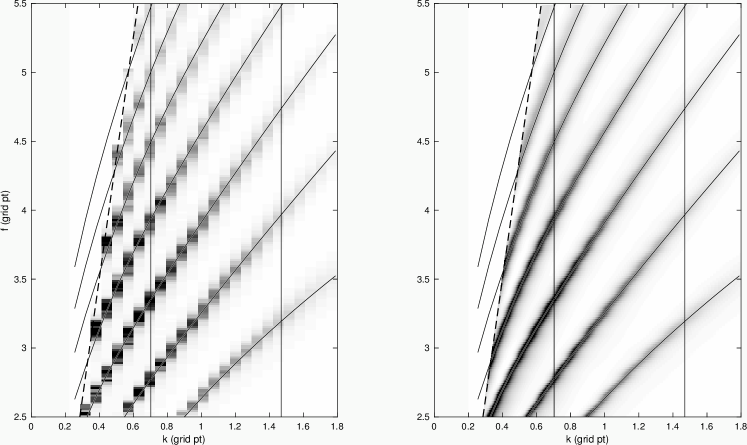
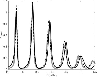
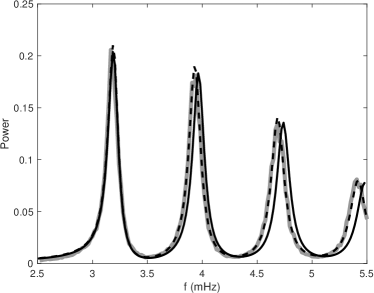
Figure 11 shows two example slices through the power spectra at constant horizontal wavenumber. In these slices, the result of the fit is shown along with the power spectra from the synthetic data and the model power spectrum from the kernel calculation. As discussed earlier, the kernel calculation is carried out using the model S stratification, and so the resonance frequencies are slightly different than in the simulations.

Figure 11: Slices through the power spectra from Figure 10 at $\ell=489$ and $\ell=1023$. The simulation power spectrum is shown in the thick gray line, the fit is the dashed black line, and the model power spectrum based on the fitted source function and linewidths, but with model S mode frequencies is shown in the solid black line.

Appendix B Flow kernels

For the calculation of the kernels, we work in a coordinate system where ${\bf r}$ is horizontal position and $z$ is height measured from the photosphere ($z=0$). The background model is translation invariant and given by a plane-parallel version of model S.

At each temporal frequency, the ingression $H_{-}$ at horizontal position ${\mathbf{r}}$ for a particular focus height $z$ is related to the observed wavefield $\phi$ by

$$H_{-}({\mathbf{r}})=\int G_{-}^{P}({\mathbf{r}}^{\prime}-{\mathbf{r}})\phi({\mathbf{r}}^{\prime})\;d{\mathbf{r}}^{\prime}$$ (B1)

where $G_{-}^{P}$ is the anti-causal Green’s function multiplied by the appropriate pupil function $P$ and data-analysis filter function. The Green’s function, the pupil function, and the filter function all depend on the focus depth (see §3). For the sake of readability, we have also suppressed the notation showing that $H_{-}$, $G_{-}$, and $\phi$ are all functions of temporal frequency. The integral is taken over all horizontal positions where the pupil function is not zero. Equation (B1) shows that the ingression is the result of filtering the wavefield with a non-axisymmetric filter (the 2D Fourier transform of $G_{-}^{P}$). The egression is related to the wavefield by an analogous equation, but with $G_{-}$ replaced by the causal Green’s function $G_{+}$, and the pupil function replaces by its appropriate counterpart (e.g, for the NS travel-time difference, if $P$ is the north pupil then $P^{\prime}$ is the south pupil).

At each temporal frequency, The lateral-vantage ingression-egression covariance $C$ at the horizontal position ${\mathbf{r}}={\bf 0}$ is

$$C({\mathbf{r}})=H^{*}_{-}({\mathbf{r}})H_{+}({\mathbf{r}})\;.$$ (B2)

The ingression-egression covariance is a time-distance covariance at zero distance (recalling the ingression and egression are filtered versions of the wavefield). We can use equations (11)-(13), which already allow for arbitrary non-axisymmetric filters, from Birch & Gizon (2007) to compute the linear sensitivity of $C$ to flows.

Travel-time shifts are measured from the ingression-egression covariance $C$ as

$$\tau={\rm Arg}\left[\bar{C}\right]/\bar{\omega}\;,$$ (B3)

where $\bar{C}$ is the sum of $C$ over all frequency bins and $\bar{\omega}$ is the average frequency weighted by $|C|$. The perturbation $\delta\tau$ to the travel-time shift coming from a perturbation $\delta\bar{C}$ to the frequency-summed ingression-egression covariance is:

$$\delta\tau={\rm Im}[\bar{C}^{*}\delta\bar{C}]/\left[|\bar{C}|^{2}\bar{\omega}\right]\;.$$ (B4)

This equations shows that the linear sensitivity of the travel-time shift to flows is a linear combination of the kernels for the ingression-egression covariances (Eq. (B2). The resulting vector-valued kernels ${\bf K}$ satisfy:

$$\delta\tau({\mathbf{r}})=\int\!\!\int\!\!\int{\bf K}({\mathbf{r}}^{\prime}-{\mathbf{r}},z)\cdot{\bf u}({\mathbf{r}}^{\prime},z)\;d{\mathbf{r}}^{\prime}dz\;.$$ (B5)

Appendix C Example kernels

Figure 12 shows slices through the kernels $K_{\beta}^{\mathrm{we}}$ for the focus depth 3.97 Mm. The kernel $K_{x}^{\mathrm{we}}$ is symmetric in both $x$ and $y$, the kernel $K_{y}^{\mathrm{we}}$ is anti-symmetric in both $x$ and $y$, and the kernel $K_{z}^{\mathrm{we}}$ is anti-symmetric in $x$ and symmetric in $y$. The $K_{x}^{\mathrm{we}}$ and $K_{z}^{\mathrm{we}}$ kernels have larger amplitudes than the $K_{y}^{\mathrm{we}}$ kernel; as expected travel-time differences in the $x$ direction are mostly sensitive to flows in the $x$ direction and vertical flows. The depth dependence of the $K_{x}^{\mathrm{we}}$ is shown in more detail in Figure 13.

Figure 12: Slices through the kernels $K_{\beta}^{\mathrm{we}}$ for a focus depth of 3.97 Mm. These kernels provide the sensitivity of the travel-time difference in the $x$ direction to arbitrary 3D flows. The left (middle, right) column shows slices through the $K_{x}^{\mathrm{we}}$ ($K_{y}^{\mathrm{we}}$, $K_{z}^{\mathrm{we}}$) kernel. The top row shows slices at the photosphere of the model and the second row shows vertical slices at $y=0$. For the case of a horizontally uniform flow, the travel-time shift would depend only on the $K_{x}^{\mathrm{we}}$ kernel.

Figure 13: The depth dependence of the horizontally-integrated kernels $K_{x}^{\mathrm{we}}$ for the different focus depths as indicated.

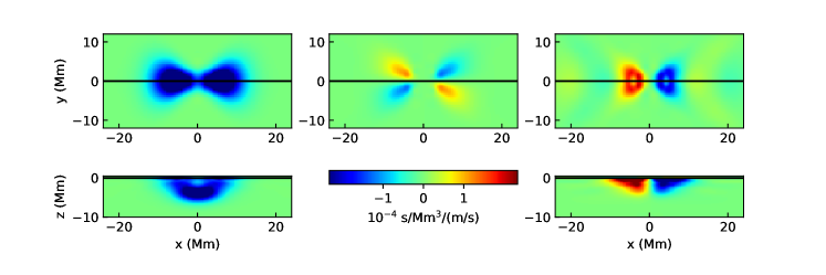
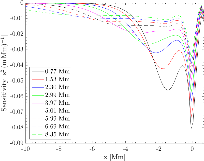
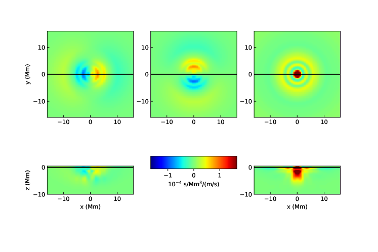
Figure 14 shows slices through the kernels $K_{\beta}^{\rm oi}$ for the focus depth 3.97 Mm. The symmetries are different than for the case of travel-time difference in the $x$ direction. The kernel $K_{x}^{\mathrm{oi}}$ is anti-symmetric in $x$ and symmetric in $y$. The kernel $K_{y}^{\mathrm{oi}}$ is symmetric in $x$ and anti-symmetric in $y$. The kernel $K_{z}^{\mathrm{oi}}$ is cylindrically symmetric about the $z$ axis. The largest sensitivity is to vertical flows near the axis. The sign is such that up-flows cause an increase in the OI time difference.

Figure 14: Slices through the kernels $K_{\beta}^{\mathrm{oi}}$ for the sensitivity of the OI travel-time difference for the focus depth of 3.97 Mm. The layout is the same as in Figure 12. The symmetries are different than in the case of the travel-time difference in the $x$ direction. In the case of OI measurements, the travel-time sensitivity is dominated by sensitivity to vertical flows near the horizontal focus point.

References

- Bhattacharya et al. (2017) Bhattacharya, J., Hanasoge, S. M., Birch, A. C., & Gizon, L. 2017, A&A, 607, A129
- Birch et al. (2009) Birch, A. C., Braun, D. C., Hanasoge, S. M., & Cameron, R. 2009, Sol. Phys., 254, 17
- Birch & Gizon (2007) Birch, A. C., & Gizon, L. 2007, Astronom. Nach., 328, 228
- Birch et al. (2004) Birch, A. C., Kosovichev, A. G., & Duvall, Jr., T. L. 2004, ApJ, 608, 580
- Braun (2014) Braun, D. C. 2014, Sol. Phys., 289, 459
- Braun (2015) —. 2015, in Extraterrestrial Seismology, ed. V. C. H. Tong & R. A. Garcia (Cambridge: Cambridge University Press), 77–90
- Braun & Birch (2008) Braun, D. C., & Birch, A. C. 2008, ApJ, 689, L161
- Braun et al. (2007) Braun, D. C., Birch, A. C., Benson, D., Stein, R. F., & Nordlund, A. 2007, ApJ, 669, 1395
- Braun et al. (2012) Braun, D. C., Birch, A. C., Rempel, M., & Duvall, Jr., T. L. 2012, ApJ, 744, 77
- Christensen-Dalsgaard (2003) Christensen-Dalsgaard, J. 2003, Lecture Notes on Stellar Oscillations, 5th edn. (Institute for Fysik og Astronomi, Aarhus Universitet)
- Christensen-Dalsgaard et al. (1996) Christensen-Dalsgaard, J., Dappen, W., Ajukov, S. V., et al. 1996, Science, 272, 1286
- DeGrave et al. (2014a) DeGrave, K., Jackiewicz, J., & Rempel, M. 2014a, ApJ, 788, 127
- DeGrave et al. (2014b) —. 2014b, ApJ, 794, 18
- Dombroski et al. (2013) Dombroski, D. E., Birch, A. C., Braun, D. C., & Hanasoge, S. M. 2013, Sol. Phys., 282, 361
- Duvall & Hanasoge (2013) Duvall, T. L., & Hanasoge, S. M. 2013, Sol. Phys., 287, 71
- Duvall et al. (2014) Duvall, T. L., Hanasoge, S. M., & Chakraborty, S. 2014, Sol. Phys., 289, 3421
- Felipe et al. (2010) Felipe, T., Khomenko, E., & Collados, M. 2010, ApJ, 719, 357
- Gizon & Birch (2004) Gizon, L., & Birch, A. C. 2004, ApJ, 614, 472
- Gizon et al. (2010) Gizon, L., Birch, A. C., & Spruit, H. C. 2010, ARA&A, 48, 289
- Hanasoge et al. (2007) Hanasoge, S. M., Duvall, Jr., T. L., & Couvidat, S. 2007, ApJ, 664, 1234
- Hartlep et al. (2008) Hartlep, T., Zhao, J., Mansour, N. N., & Kosovichev, A. G. 2008, ApJ, 689, 1373
- Howe (2009) Howe, R. 2009, Liv Rev Solar Phys, 6, doi:10.1007/lrsp-2009-1
- Jackiewicz et al. (2012) Jackiewicz, J., Birch, A. C., Gizon, L., et al. 2012, Sol. Phys., 276, 19
- Lindsey & Braun (1997) Lindsey, C., & Braun, D. C. 1997, ApJ, 485, 895
- Lindsey & Braun (2004) —. 2004, ApJS, 155, 209
- Parchevsky & Kosovichev (2007) Parchevsky, K. V., & Kosovichev, A. G. 2007, ApJ, 666, 547
- Parchevsky et al. (2014) Parchevsky, K. V., Zhao, J., Hartlep, T., & Kosovichev, A. G. 2014, ApJ, 785, 40
- Pijpers & Thompson (1992) Pijpers, F. P., & Thompson, M. J. 1992, A&A, 262, L33
- Rempel (2014) Rempel, M. 2014, ApJ, 789, 132
- Rempel (2015) —. 2015, ApJ, 814, 125
- Rempel et al. (2009) Rempel, M., Schüssler, M., & Knölker, M. 2009, ApJ, 691, 640
- Stein & Nordlund (2012) Stein, R. F., & Nordlund, Å. 2012, ApJ, 753, L13
- Stein et al. (2009) Stein, R. F., Nordlund, Å., Georgoviani, D., Benson, D., & Schaffenberger, W. 2009, in Solar-Stellar Dynamos as Revealed by Helio- and Asteroseismology: GONG 2008/SOHO 21, ed. M. Dikpati, T. Arentoft, I. González Hernández, C. Lindsey, & F. Hill, Vol. 416 (San Francisco: Astron. Soc. Pacific), 421
- Švanda (2012) Švanda, M. 2012, ApJ, 759, L29
- Švanda (2013) —. 2013, ApJ, 775, 7
- Švanda (2015) —. 2015, A&A, 575, A122
- Švanda et al. (2011) Švanda, M., Gizon, L., Hanasoge, S. M., & Ustyugov, S. D. 2011, A&A, 530, A148
- Zhao et al. (2007) Zhao, J., Georgobiani, D., Kosovichev, A. G., et al. 2007, ApJ, 659, 848