Surface plasmon launching by polariton superradiance

Abstract

The condition of phase matching prohibits the transfer of excitation from free-space photons to surface plasmon polaritons (SPP). We propose and analyze a scheme that excites an ensemble of emitters in a collective state, which is phase matched with the SPP by the optical pulses used for its preparation. By a collective enhancement the ensemble, hence, emits an SPP in a well defined direction. We demonstrate the scheme by analyzing the launching of near-infrared graphene SPP. Our theory incorporates the dispersive and dissipative properties of the plasmon modes to evaluate the non-Markovian emission by the ensembles and will also be applicable for other types of surface polaritons.

Surface plasmon polaritons (SPPs) are electromagnetic modes confined at metal-dielectric interfaces Novotny and Hecht (2012) or near two-dimensional materials such as graphene Grigorenko et al. (2012). SPPs have dispersion relations different from the ones of free space photons. This difference, occurring also for phonon polaritons Hillenbrand et al. (2002); Taubner et al. (2006); Dai et al. (2014); Li and Nori (2018), exciton polaritons Low et al. (2016); Basov et al. (2016) and surface polaritons in heterostructures Lin et al. (2017); Woessner et al. (2014), leads to a wavenumber mismatch and prevents their effective production by conversion from free-space photons. To close the mismatch and launch SPPs, conventional methods use prisms within the Otto configuration Otto (1968) or the Kretschmann configuration Kretschmann (1971) to shorten the photon wavelength, or they equip the SPP dispersion relation with band structure by using grating couplers Raether (1988), or lengthen the SPP wavelength with an atomic gas medium Du et al. (2015). The excitation of graphene SPP is more challenging because the wavelength of graphene SPP (THz to near-infrared regimes) is two orders of magnitude smaller than that of free-space light of the same frequency Koppens et al. (2011). Special techniques use scattering resonances of nanoantennas Krasnok et al. (2018); Alonso-González et al. (2014); Gao et al. (2012, 2013) or near-field sources Fei et al. (2012); Chen et al. (2012), and optical methods, based on the intrinsic nonlinear interaction of graphene with light Constant et al. (2015), have realized launching of graphene SPPs in THz to mid-infrared regimes.

In this Letter, we will investigate the prospects of SPP launching by an emitter ensemble. A single localized two-level quantum emitter may, indeed, absorb an optical photon and subsequently emit an SPP by spontaneous emission Akimov et al. (2007); Tame et al. (2013); Tielrooij et al. (2015). For a point source there is no issue of wavenumber mismatch, but also no control of the directionality of the launched SPP. Excitation of SPP with a single wavenumber and direction is vital for many applications López-Tejeira et al. (2007); Lin et al. (2013); Pors et al. (2014); You et al. (2015); Krasnok et al. (2018); Bliokh et al. (2018); Song and Rudner (2017); Andolina et al. (2018). Our proposal applies a train of $\pi$-pulses to write a wave vector into the phase of the spin wave excitation of the emitter ensemble, which is phase matched with the SPP with the desired directionality (determined by the wave vectors of the $\pi$-pulses). While we will demonstrate the scheme for a near-infrared graphene SPP, the theory works for a broad range of SPPs and will be applicable also to other surface polaritons Hillenbrand et al. (2002); Taubner et al. (2006); Dai et al. (2014); Li and Nori (2018); Low et al. (2016); Basov et al. (2016); Lin et al. (2017); Woessner et al. (2014).

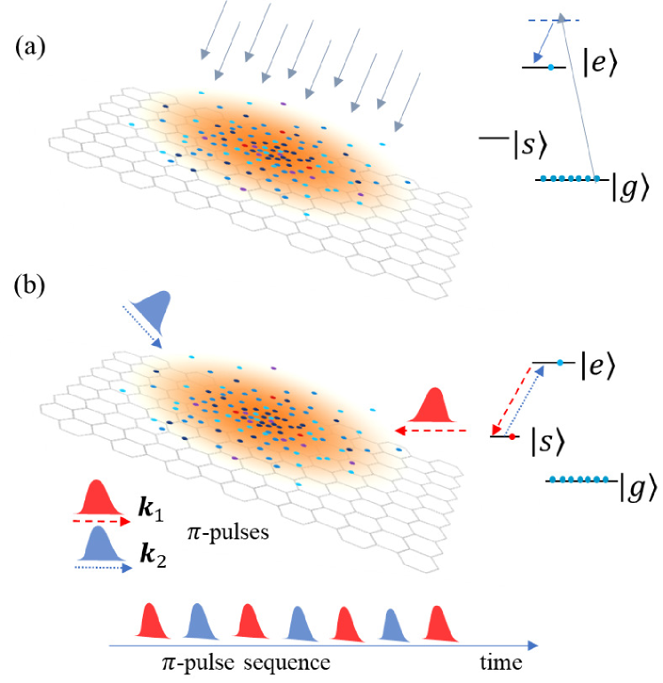
Figure 1: Scheme for preparation of an SPP phase matched timed-Dicke state. (a) Raman excitation of one of the emitters into the excited state $|e\rangle$, using uniform optical illumination perpendicular to the surface. (b) Illumination by a train of $\pi$-pulses on the $\ket{s}\leftrightarrow\ket{e}$ transition, driving the emitters to the target timed-Dicke state $|\psi_{\mathbf{k}_{sp}}\rangle$.

When a photon is absorbed by a single emitter, the information of its wave vector is lost and has no impact on following emission processes. However, if the photon is uniformly absorbed by an ensemble of $N$ emitters, its wave vector $\mathbf{k}$ is recorded by the emitters in the phases of the so-called timed-Dicke state Scully et al. (2006),

$$|\psi_{\mathbf{k}}\rangle=\frac{1}{\sqrt{N}}\sum_{a=1}^{N}\;e^{i\mathbf{k}\cdot\mathbf{r}_{a}}|s_{a}\rangle\bigotimes_{b\neq a}|g_{b}\rangle,$$ (1)

where $|g\rangle$ is the emitter ground state, $|s\rangle$ is an excited state, and $\mathbf{r}_{a}$ is the position of the $a^{th}$ emitter. In analogy with single-photon superradiance Scully and Svidzinsky (2009) if $|s\rangle$ couples to the SPP field, spontaneous emission from $|\psi_{\mathbf{k}}\rangle$ generates a polariton excitation with wave vector $\simeq\hbar\mathbf{k}$ and energy $\simeq\hbar\omega_{sg}=E_{s}-E_{g}$ Scully et al. (2006). Directional SPP launching based on this process is possible only if $|\psi_{\mathbf{k}_{sp}}\rangle$ is prepared with the appropriate SPP wave vector $\mathbf{k}_{sp}$, such that the SPP frequency $\omega_{\mathbf{k}_{sp}}=\omega_{sg}$. This can be accomplished by Raman processes via a third atomic level $\ket{e}$, see Fig. 1.

Preparation of $|\psi_{\mathbf{k}_{sp}}\rangle$-We consider the simple case where SPPs are confined to an infinite plane interface, above which a parallel thin layer of emitters is deposited. The preparation of $|\psi_{\mathbf{k}_{sp}}\rangle$ proceeds by two steps.

1. A single quantum is uniformly absorbed by a Raman process $|g\rangle\rightarrow|e\rangle$ transition, e.g., following the heralded scheme Scully et al. (2006); Scully and Svidzinsky (2009) (the case of more excitations is discussed below). Applying optical fields propagating perpendicular to the emitter layer, see Fig 1(a), the collectively shared excitation has no phase variation across the ensemble.

2. A train of $(2n_{p}+1)$ $\pi$-pulses resonant with the $|e\rangle$-$|s\rangle$ transition bounces the state amplitude of the emitters back and forth between $|e\rangle$ and $|s\rangle$, while the in-plane wave-vectors $\mathbf{k}_{1}$ or $\mathbf{k}_{2}$, see Fig. 1(b), cause accumulation of a wave vector that we design to satisfy the equality $-(n_{p}+1)\mathbf{k}_{1}+n_{p}\mathbf{k}_{2}=\mathbf{k}_{sp}$.

The combination of these processes produces the desired timed-Dicke state $|\psi_{\mathbf{k}_{sp}}\rangle$ Wang and Scully (2014). For schemes based on emissions from $|\psi_{\mathbf{k}_{sp}}\rangle$, two apparent contradictory requirements must be addressed: To make the superradiant emission dominate the incoherent emissions, the ensemble should be optically thick for the emitted mode Berman and Le Gouët (2011); Röhlsberger et al. (2010); Roof et al. (2016), while the presumed uniform optical excitation requires the ensemble to be optically thin during the state preparation Scully (2007). We can indeed satisfy both conditions simultaneously: The optical processes are either driven orthogonally to the thin emitter ensemble or they act on only a single emitter population (of states $\ket{e}$ and $\ket{s}$), thus the system is optically thin. The emission modes here are SPP modes propagating parallel to the emitter layer, and the SPP-emitter interaction is collectively enhanced by the large number of atoms in the final internal state $\ket{g}$. Thus, the system may be optically thick upon emission.

The state $|e\rangle$ is coupled to $|g\rangle$ by a two-photon Raman process, and the collectively shared excitation in $|e\rangle$ may hence be stable against spontaneous decay to the atomic ground state $|G\rangle=|g_{1},g_{2},\cdots g_{N}\rangle$. During Step 2, until we have completed the pulse train, the intermediate timed-Dicke states $|\psi_{-(n+1)\mathbf{k}_{1}+n\mathbf{k}_{2}}\rangle$ ($n<n_{p}$) have energy $\hbar\omega_{sg}$ but wavenumber smaller than $k_{sp}$ while larger than the free-space resonant wavenumber $\omega_{sg}/c$. These intermediate states may be protected from decaying and emitting to SPP or free-space fields due to the wave number mismatch. Thus our scheme works if the intermediate state lifetime supplies enough time window for the $\pi$-pulses.

The length of the pulse train depends on the ratio between the wavelength of optical photons ($\lambda_{es}$) and the SPP wavelength ($\lambda_{sp}$), $2n_{p}+1\simeq\lambda_{es}/\lambda_{sp}$. For the values of $\lambda_{sp}$, graphene SPP may serve as an example. Graphene SPPs are distinguished by their tight confinement and long lifetime, and by their high tunability via electrostatic gating Koppens et al. (2011); Grigorenko et al. (2012). For SPPs with frequency $\hbar\omega<2E_{f}$ García de Abajo (2014) where $E_{f}\leq 1\mathrm{eV}$ is the Fermi energy, the graphene surface conductivity is approximated by the Drude conductivity: $\sigma_{g}(\omega)\approx i\frac{e^{2}}{\pi\hbar^{2}}E_{f}/(\omega+i\tau_{D}^{-1})$. The value of $\tau_{D}$ currently available in experiments is $0.5\,\mathrm{ps}$ Woessner et al. (2014), while it may intrinsically reach values of $10^{2}\,\mathrm{ps}$ Principi et al. (2013). Supposing for simplicity a vacuum below and above the graphene monolayer, the dispersion relation of the p-mode graphene SPP is $\omega_{sp}=\sqrt{2\alpha cE_{f}k_{sp}/\hbar}$, where $\alpha\approx 1/137$ is the fine-structure constant. Supposing $E_{f}=0.5\,$eV, then for $\hbar\omega_{sp}\in[0.01\,\mathrm{eV},1\,\mathrm{eV}]$ Principi et al. (2013) $\lambda_{sp}$ ranges from 90 $\mathrm{\mu m}$ to 18 nm.

For optical pulses $\lambda_{es}\in[380\,\mathrm{nm},750\,\mathrm{nm}]$, the number of pulses $2n_{p}+1\simeq\lambda_{es}/\lambda_{sp}<50$ and even a single pulse is sufficient for low-energy SPPs with $\lambda_{sp}>\lambda_{es}$. We can drive the optical $\pi$-pulses on the time scale of nanoseconds using pulse powers that are far from damaging graphene Kiisk et al. (2013) and other surface polariton systems.

The validity of this scheme replies on details of the collective emitter-SPP coupling to be analyzed in the following. We will first focus on the emission from $|\psi_{\mathbf{k}_{sp}}\rangle$. Then we will study the decay of the intermediate states, which should be suppressed in order to successfully prepare $|\psi_{\mathbf{k}_{sp}}\rangle$. Our analysis will clarify the proper regime for the experimental parameters.

Emitter-SPP Coupling-To study the emission from the prepared state $|\psi_{\mathbf{k}_{sp}}\rangle$, we now turn to the coupling to the dispersive and dissipative electric field quantized as Dung et al. (1998); Philbin (2010); Gruner and Welsch (1996)

$$\mathbf{E}(\mathbf{r}_{a})=i \mu_{0}\sqrt{\frac{\hbar\epsilon_{0}}{\pi}}\int_{0}^{\infty}d\tilde{\omega}\int d^{3}\mathbf{r}^{\prime}\tilde{\omega}^{2}\sqrt{\Im\epsilon(\mathbf{r}^{\prime},\tilde{\omega})}$$ (2)

$$\times\mathbf{G}(\mathbf{r}_{a},\mathbf{r}^{\prime},\tilde{\omega})\cdot\mathbf{f}(\mathbf{r}^{\prime},\tilde{\omega})+h.c.,$$

where $\mu_{0}$ and $\epsilon_{0}$ are the vacuum susceptibility and permittivity; $\Im\epsilon(\mathbf{r}^{\prime},\tilde{\omega})$ is the imaginary part of the relative permittivity; $\mathbf{G}(\mathbf{r},\mathbf{r^{\prime}},\tilde{\omega})$ is the dyadic Green’s tensor determined by Maxwell’s equations, and the field $\mathbf{f}(\mathbf{r}^{\prime},\tilde{\omega})$ with three Cartesian operator components $f_{j}$ obeys the bosonic commutator relations $[f_{j},f_{k}]=0$, $[f_{j}^{\dagger},f_{k}^{\dagger}]=0$ and $[f_{j}(\mathbf{r}_{1},\tilde{\omega}_{1}),f^{\dagger}_{k}(\mathbf{r}_{2},\tilde{\omega}_{2})]=\delta_{jk}\delta(\mathbf{r}_{1}-\mathbf{r}_{2})\delta(\tilde{\omega}_{1}-\tilde{\omega}_{2})$.

The Hamiltonian is written as $H=\sum_{a=1}^{N}[\frac{1}{2}\hbar\omega_{sg}\sigma_{a}^{z}-\sigma_{a}^{x}\mathbf{d}_{a}\cdot\mathbf{E}(\mathbf{r}_{a})]+\int d^{3}\mathbf{r^{\prime}}\int_{0}^{\infty}d\tilde{\omega}\,\hbar\tilde{\omega}\mathbf{f}^{\dagger}(\mathbf{r^{\prime}},\tilde{\omega})\mathbf{f}(\mathbf{r^{\prime}},\tilde{\omega})$ where $\mathbf{d}_{a}$ is the dipole of the $|g_{a}\rangle$-$|s_{a}\rangle$ transition, $\sigma^{z}_{a}=|s_{a}\rangle\langle s_{a}|-|g_{a}\rangle\langle g_{a}|$ and $\sigma^{x}_{a}=|s_{a}\rangle\langle g_{a}|+|g_{a}\rangle\langle s_{a}|$. Here and throughout, $\hbar=1$. We shall use the rotating-wave approximation and study the evolution based on the ansatz written with time-dependent amplitudes $\alpha_{a}$ and $\beta_{a}(\tilde{\omega},\mathbf{r}^{\prime})$:

$$|\Psi\rangle=\sum_{a=1}^{N}\alpha_{a}|s_{a},{\varnothing}\rangle\bigotimes_{b\neq a}|g_{b}\rangle+\int_{j,\tilde{\omega},\mathbf{r}^{\prime}}\beta_{j}(\tilde{\omega},\mathbf{r}^{\prime})|G,1_{j,\tilde{\omega},\mathbf{r}^{\prime}}\rangle$$ (3)

where $|{\varnothing}\rangle$ is the field vacuum state, $|1_{j,\tilde{\omega},\mathbf{r}^{\prime}}\rangle=f_{j}^{\dagger}(\mathbf{r}^{\prime},\tilde{\omega})|{\varnothing}\rangle$ and $\int_{j,\tilde{\omega},\mathbf{r}^{\prime}}$ is the short hand for $\sum_{j}\int d\tilde{\omega}\int d^{3}\mathbf{r}^{\prime}$. The strength of the emitter-emitter coupling mediated by all environmental modes

$$g_{ab}(\tilde{\omega})=\frac{\mu_{0}}{\pi}\tilde{\omega}^{2}\mathbf{d}_{a}\cdot\mathbf{G}(\mathbf{r}_{a},\mathbf{r}_{b},\tilde{\omega})\cdot\mathbf{d}_{b}$$ (4)

has the symmetry $g_{ab}(\tilde{\omega})=g_{ba}(\tilde{\omega})$. Due to the in-plane translation symmetry (we assume that the dipoles of the emitters are identical)Novotny and Hecht (2012), $g_{ab}(\tilde{\omega})$ can be expanded in the wave number representation

$$g_{ab}(\tilde{\omega})=\int\frac{\mathbf{d^{2}k_{\shortparallel}}}{(2\pi)^{2}}\,g_{z_{a},z_{b}}(\tilde{\omega},\mathbf{k_{\shortparallel}})e^{i\mathbf{k_{\shortparallel}}\cdot(\mathbf{r}_{a}-\mathbf{r}_{b})},$$ (5)

where the subindex “$z_{a},z_{b}$” indicates the emitter heights above the interface. For a thin emitter layer, we approximate all the emitter $z$-coordinates by a single value $z_{at}$, and we thus express $g_{z_{a},z_{b}}(\tilde{\omega},\mathbf{k_{\shortparallel}})$ as $g_{z_{at}}(\tilde{\omega},\mathbf{k_{\shortparallel}})$.

Similarly, the excitation amplitudes of the individual emitters defined in Eq. (3) can also be transformed into wave number representation, i.e., $\alpha_{\mathbf{k}_{\shortparallel}}(t)=\langle\psi_{\mathbf{k}_{\shortparallel}},{\varnothing}|\Psi(t)\rangle$, which follows the equation

$$-\partial_{t}\alpha_{\mathbf{k}_{\shortparallel}} (t)=N\int\frac{d^{2}\mathbf{q}_{\shortparallel}}{(2\pi)^{2}}\int_{\tilde{\omega}}\Im g_{z_{at}}(\tilde{\omega},\mathbf{q}_{\shortparallel})\zeta(\mathbf{k}_{\shortparallel},\mathbf{q}_{\shortparallel})$$ (6)

$$\quad\times\int_{0}^{t}d\tau\alpha_{\mathbf{q}_{\shortparallel}}(\tau)e^{-i(\tilde{\omega}-\omega_{sg})(t-\tau)}$$

where $\Im$ denotes the imaginary part and

$$\zeta(\mathbf{q}_{\shortparallel},\mathbf{k}_{\shortparallel})=\langle\psi_{\mathbf{q}_{\shortparallel}}|\psi_{\mathbf{k}_{\shortparallel}}\rangle$$ (7)

is a geometry factor which quantifies the sharpness of the phase matching condition given the spatial distribution of the emitters. If $N\gg 1$ and the emitters are for example distributed independently according to a Gaussian distribution with width $L$, $\zeta(\mathbf{k}_{\shortparallel},\mathbf{q}_{\shortparallel})=e^{-L^{2}(\mathbf{k}_{\shortparallel}-\mathbf{q}_{\shortparallel})^{2}/2}$.

The factor of $N$ in Eq. (6) demonstrates the effect of collective enhancement. The collective Lamb shift of state $|\psi_{\mathbf{k}_{sp}}\rangle$ should be considered unless it is smaller than the line width of the SPP mode. For completeness, we provide the expressions for the collective Lamb shift in the Supporting Information.

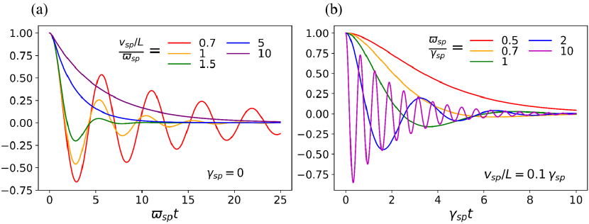
Figure 2: Evolution of $\alpha_{\mathbf{k}_{sp}}(t)$ determined by Eq. (9). (a) $\varpi_{sp}$ and $\lambda_{sp}$ are fixed while $v_{sp}/L$ is varied. (b) $v_{sp}/L$ and $\gamma_{sp}$ are fixed while $\varpi_{sp}$ is varied.

Evolution of $\ket{\psi_{\mathbf{k}_{sp}}}$-To analyze the evolution described by Eq. (6), we shall start from the initial state $|\psi_{\mathbf{k}_{sp}},\varnothing\rangle$ and focus on the state amplitude $\alpha_{\mathbf{k}_{sp}}(t)$. $|\psi_{\mathbf{k}_{sp}}\rangle$ resonantly matches the SPP with frequency $\omega_{sg}$ while phase-matched photon modes are off-resonant. Thus we may consider only the coupling to a range of SPPs. We use $\omega_{\mathbf{k}_{\shortparallel}}$ and $\gamma_{\mathbf{k}_{\shortparallel}}$ to denote the frequency and damping rate of the SPP with in-plane momentum $\mathbf{k}_{\shortparallel}$. They are determined by the position of the pole of $g_{z,z^{\prime}}(\tilde{\omega},\mathbf{k}_{\shortparallel})$ in the complex $\tilde{\omega}$ plane Novotny and Hecht (2012). Keeping only the contribution from the poles leads to a Lorentzian type expression

$$\Im g_{z,z^{\prime}}(\tilde{\omega},\mathbf{k}_{\shortparallel})\approx\frac{A_{z,z^{\prime}}(\mathbf{k}_{\shortparallel})\gamma_{\mathbf{k}_{\shortparallel}}}{(\tilde{\omega}-\omega_{\mathbf{k}_{\shortparallel}})^{2}+\gamma_{\mathbf{k}_{\shortparallel}}^{2}},$$ (8)

where $A_{z,z^{\prime}}(\mathbf{k}_{\shortparallel})$ is fixed by the residue of $g_{z,z^{\prime}}(\tilde{\omega},\mathbf{k}_{\shortparallel})$ at the pole $\tilde{\omega}=\omega_{\mathbf{k}_{\shortparallel}}-i\gamma_{\mathbf{k}_{\shortparallel}}$.

When $\zeta(\mathbf{k}_{\shortparallel},\mathbf{k}_{sp})$ peaks sharply at $\mathbf{k}_{\shortparallel}=\mathbf{k}_{sp}$, the distribution of the emitter excitation is centered at $|\psi_{\mathbf{k}_{sp}}\rangle$ so that $\alpha_{\mathbf{k}_{\shortparallel}}(t)\approx\langle\psi_{\mathbf{k}_{\shortparallel}}|\psi_{\mathbf{k}_{sp}}\rangle\langle\psi_{\mathbf{k}_{sp}},{\varnothing}|\Psi\rangle=\alpha_{\mathbf{k}_{sp}}(t)\zeta(\mathbf{k}_{\shortparallel},\mathbf{k}_{sp})$. This approximation makes it possible to obtain a closed equation of evolution for $\alpha_{\mathbf{k}_{sp}}$, which, with the Gaussian distribution of emitters and the corresponding geometry factor, is written as

$$-\partial_{t}\alpha_{\mathbf{k}_{sp}}=\varpi_{sp}^{2}\int_{0}^{t}d\tau\,\alpha_{\mathbf{k}_{sp}}(\tau)e^{-\frac{\mathbf{v}_{sp}^{2}}{4L^{2}}(t-\tau)^{2}-\gamma_{sp}(t-\tau)},$$ (9)

where $\varpi_{sp}^{2}=\frac{N}{4L^{2}}A_{z_{at}}(\mathbf{k}_{sp})$, and $\mathbf{v}_{sp}=\nabla_{\mathbf{k}_{\shortparallel}}\omega_{\mathbf{k}_{\shortparallel}}|_{\mathbf{k}_{\shortparallel}=\mathbf{k}_{sp}}$ is the SPP group velocity. Unlike the case of free-photon superradiance Svidzinsky et al. (2008), here the finite SPP lifetime due to Ohmic damping must be considered. We assume the SPP decay rate as a constant $\gamma_{\mathbf{k}_{\shortparallel}}=\gamma_{sp}$. For the Drude model of graphene mentioned above, $\gamma_{sp}=0.5\,\tau_{D}^{-1}$. See the Supporting Information for the derivation of Eq. (9).

The solution to Eq. (9) behaves as damped oscillations or pure decay depending on the interplay between three parameters, viz., $\varpi_{sp}$, $\gamma_{sp}$ and $v_{sp}/L$. The damped oscillation regime appears when $\varpi_{sp}$, which is roughly the frequency of the oscillation, dominates the other two parameters. To understand this condition, note that the oscillation refers to the periodical absorption and reemission of the single-SPP pulse. This process is possible only until the propagating pulse leaves the ensemble at $t\simeq L/v_{sp}$ or has been absorbed by the material due to Ohmic loss at $t\simeq\gamma_{sp}^{-1}$. In Fig. 2(a) we show the solution of Eq. (9) as function of time for different values of the finite duration $L/v_{sp}$ of the SPP pulse propagation in the emitter ensemble. Figure 2(b) shows the similar results when the damping is mainly determined by the finite SPP lifetime, $\gamma_{sp}^{-1}$. Both plots of Fig. 2 confirm the role of $\varpi_{sp}$ as oscillation frequency. In the pure decay regime ($\varpi_{sp}<\gamma_{sp},v_{sp}/L$), we obtain the Markov approximation by assuming $\alpha_{\mathbf{k}_{sp}}(\tau)=\alpha_{\mathbf{k}_{sp}}(t)$ in the right hand side of Eq. (9). It yields the decay rate

$$\Gamma_{c}=\sqrt{\pi}\frac{\varpi_{sp}^{2}}{v_{sp}/L}e^{(\frac{\gamma_{sp}}{v_{sp}/L})^{2}}\mathrm{erfc}(\frac{\gamma_{sp}}{v_{sp}/L}).$$ (10)

This expression verifies our observations in Fig. 2, e.g., that larger $\varpi_{sp}$ and $v_{sp}/L$ result in faster decay. When $v_{sp}/L$ can be neglected, $\Gamma_{c}\approx\varpi_{sp}^{2}/\gamma_{sp}<\gamma_{sp}$.

Both the damped oscillation and pure decay regimes are achievable in experiments. With realistic parameters $\omega_{sg}=E_{f}=0.5\,\mathrm{eV}$, the SPP group velocity is roughly $v_{sp}=10^{-2}c$. so that for $L\geq 1\,\mathrm{\mu m}$, $v_{sp}/L\leq 10^{12}\,\mathrm{Hz}=\gamma_{sp}$. For emitter vacuum decay rate $10^{2}\,\mathrm{MHz}$ (governed by the transition dipole moment), emitter-graphene distance $z_{at}=10\,\mathrm{nm}$ and emitter number density $n_{at}=N/L^{2}=(0.1/\mathrm{nm})^{2}$, the damped oscillation regime is reached with $\varpi_{sp}\approx 10^{14}\,\mathrm{Hz}\gg\gamma_{sp},v_{sp}/L$, see Methods. The pure decay regime can be realized by larger distance $z_{at}$, lower density $n_{at}$, or a smaller transition dipole moment.

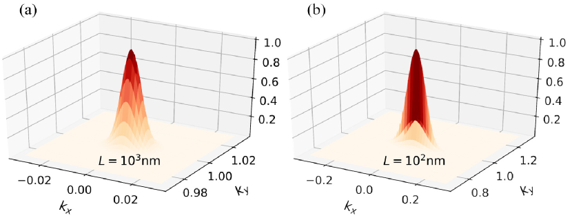
Figure 3: $P(\mathbf{k}_{\shortparallel},\omega_{sp})/P(\mathbf{k}_{sp},\omega_{sp})$ for graphene SPPs when $\omega_{sp}=E_{f}=0.5\,\mathrm{eV}$, $\tau=1\,\mathrm{ps}$, emitter-graphene distance $z_{at}=10\,\mathrm{nm}$, ensemble size (a) $L=10^{3}\,\mathrm{nm}$; (b) $L=10^{2}\,\mathrm{nm}$. $\mathbf{k}_{sp}$ is set to along $\hat{y}$-direction. The unit of the wave number is $k_{sp}$ of which the SPP wavelength is $\lambda_{sp}=36.2\,\mathrm{nm}$.

Directionality of the emitted SPP- The amplitudes $\beta_{j}(\tilde{\omega},\mathbf{r}^{\prime})$ defined in Eq. (3) can be transformed into wave number representation $\beta_{j}(\tilde{\omega},\mathbf{k}_{\shortparallel},z^{\prime})$. Although exact solutions are not accessible, we may assume a uniform decay ansatz $\alpha_{a}(t)=\alpha_{a}(0)e^{-\gamma t}$, with which the electromagnetic frequency-wave number excitation distribution $P(\mathbf{k}_{\shortparallel},\tilde{\omega})\equiv\int dz^{\prime}\sum_{j}|\beta_{j}(\tilde{\omega},\mathbf{k}_{\shortparallel},z^{\prime})|^{2}$, is

$$P(\mathbf{k}_{\shortparallel},\tilde{\omega})=\frac{N\Im g_{z_{at}}(\tilde{\omega},\mathbf{k}_{\shortparallel})|\zeta(\mathbf{k}_{sp},\mathbf{k}_{\shortparallel})|^{2}}{\gamma^{2}+(\tilde{\omega}-\omega_{sg})^{2}}.$$ (11)

Both the pole structure of $g_{z}(\tilde{\omega},\mathbf{k}_{\shortparallel})$ and the geometry factor $\zeta(\mathbf{k}_{sp},\mathbf{k}_{\shortparallel})$ in this formula guarantee the emission to peak sharply at $\mathbf{k}_{\shortparallel}=\mathbf{k}_{sp}$. The ratio between $P(\mathbf{k}_{\shortparallel},\omega_{sp})$ and the peak value $P(\mathbf{k}_{sp},\omega_{sp})$ is depicted in Fig. 3. The figure confirms that the larger ensemble size leads to stronger directionality.

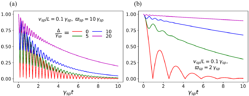
Figure 4: Evolution of $|\alpha_{\mathbf{q}_{n}}(t)|$ of the intermediate states with varying values of $\Delta$. $v_{sp}/L=0.1\,\gamma_{sp}$, (a)$\varpi_{sp}=10\,\gamma_{sp}$, (b)$\varpi_{sp}=2\,\gamma_{sp}$.

Evolution of Intermediate States-Now we turn to the intermediate states $|\psi_{\mathbf{q}_{n}}\rangle$ that may be populated for nanoseconds during Step 2 in the preparation of $|\psi_{\mathbf{k}_{sp}}\rangle$, where $\mathbf{q}_{n}=-(n+1)\mathbf{k}_{1}+n\mathbf{k}_{2}$ ($0\leq n<n_{p}$). Since $\omega_{es}>\omega_{sg}$ and $\omega_{sg}/c<q_{n}<k_{sp}$, the photon and SPP modes matching the wave vector $q_{n}\simeq(2n+1)\omega_{es}/c$ are not resonant with $\omega_{sg}$. We denote the two detunings as $\Delta_{n}=\omega_{sg}-\omega_{\mathbf{q}_{n}}$ and $\Delta_{n}^{(0)}=cq_{n}-\omega_{sg}$, respectively. For $\omega_{es}$ in the optical regime and graphene SPP frequency $\omega_{sg}$ at most in the near-infrared, $\Delta_{n}^{(0)}\gg\Delta_{n}$ ($\Delta_{n}^{(0)}$ ranges from optical to ultraviolet frequencies) thus we can disregard the coupling to free-space photons. Then the equation of evolution for $\alpha_{\mathbf{q}_{n}}(t)$ resembles Eq. (9) but with the replacement $\gamma_{sp}\rightarrow\gamma_{sp}+i\Delta_{n}$ and $\varpi_{sp},v_{sp}$ should be defined by the wave vector $\mathbf{q}_{n}$ (see the Supplemental Material for the full formulae). In the damped oscillation regime, we illustrate the solution to $|\alpha_{\mathbf{q}_{n}}|$ in Fig. 4. It shows that compared with the phase-matched case ($\Delta_{n_{p}}=0$), the intermediate states have longer lifetime, especially when $\varpi_{sp}$ is smaller.

In the pure decay regime, the Markov approximation yields the decay rate of $|\psi_{\mathbf{q}_{n}}\rangle$,

$$\Gamma_{\mathbf{q}_{n}}=\frac{\varpi_{sp}^{2}}{\gamma_{sp}^{2}+\Delta_{n}^{2}}\gamma_{sp},$$ (12)

where we have omitted terms of order $v_{sp}/L$ that are dominated by $\gamma_{sp}$ in a large ensemble. Since $\gamma_{sp}$ is the uncertainty of the SPP frequency, in practice we would require $\Delta_{n}\gg\gamma_{sp}$. For near-infrared graphene SPP with $\hbar\omega_{sp}=E_{f}=0.5\,\mathrm{eV}$ and wavelength $\lambda_{sp}=36.2\,\mathrm{nm}$, supposing optical pulse wavelength $\lambda_{es}=500\,\mathrm{nm}$, 15 pulses are sufficient to prepare $\ket{\psi_{\mathbf{k}_{sp}}}$ and $\Delta_{n}\geq\Delta_{n_{p}-1}\approx 0.035\,\mathrm{eV}\approx 10\gamma_{sp}$ for all intermediate states $\ket{\psi_{\mathbf{q}_{n}}}$ with $n<n_{p}$. Equation (12) implies that when $\varpi_{sp}<0.1\gamma_{sp}$, $|\psi_{\mathbf{q}_{n_{p}-1}}\rangle$ has a lifetime longer than $10^{4}\gamma_{sp}^{-1}=10\,\mathrm{ns}$, allowing its population for $\leq$ 1 $\mathrm{ns}$ during the last two $\pi$-pulses required to prepare $\ket{\psi_{\mathbf{k}_{sp}}}$.

In the damped oscillation regime, however, the lifetime of the intermediate states may be too short to facilitate the preparation of $|\psi_{\mathbf{k}_{sp}}\rangle$. In this case, we may employ another metastable emitter level $|s^{\prime}\rangle$ which disallows the direct $\ket{s^{\prime}}$-$\ket{g}$ transition. The SPP wave number is then accumulated with the $\ket{e}$-$\ket{s^{\prime}}$ transition and a final pulse moves the collective excitation from $\ket{s^{\prime}}$ to $\ket{s}$ to obtain $\ket{\psi_{\mathbf{k}_{sp}}}$.

Conclusions and Discussions-We have proposed to prepare an emitter ensemble into collective states that match the wave vector of surface plasmon polaritons and hence directionally emit SPPs via polariton superradiance. The directionality has high tunability, i.e., the direction is determined simply by the wave vectors of the $\pi$-pulses used in the preparation of the timed-Dicke states. We studied the evolution of the collective emitter excitation and showed that the intermediate states have lifetime long enough to implement the required pulses sequence. With the Drude model parameters of graphene SPP in the near-infrared regime, we predict excellent directionality of launching. Our main general formalism also applies to other families of surface polaritons Hillenbrand et al. (2002); Taubner et al. (2006); Dai et al. (2014); Low et al. (2016); Li and Nori (2018); Basov et al. (2016); Lin et al. (2017); Woessner et al. (2014).

In the end, we emphasize that the requirement of only a single excitation in the timed-Dicke state can be released to the low-excitation regime. In this regime, the spin operators can be approximated with bosonic ladder operators $\sigma^{-}_{a}\rightarrow\hat{b}_{a}$. We can translate them into momentum representation by $\hat{b}_{\mathbf{q}_{\shortparallel}}=\frac{1}{\sqrt{N}}\sum_{a=1}^{N}\hat{b}_{a}e^{-i\mathbf{q}_{\shortparallel}\cdot\mathbf{r}_{a}}$ with $[\hat{b}_{\mathbf{q}_{\shortparallel}},\hat{b}_{\mathbf{k}_{\shortparallel}}^{\dagger}]=\zeta(\mathbf{q}_{\shortparallel},\mathbf{k}_{\shortparallel})\approx\delta_{\mathbf{q}_{\shortparallel},\mathbf{k}_{\shortparallel}}$, The weak coherent state amplitudes then obey similar equations as the single excitation amplitudes in Eq. (3) Porras and Cirac (2008). For a system with inhomogeneous broadening, for example, doped rare-earth ions in crystals, the $\pi$-pulses should be implemented in a more sophisticated way Remizov et al. (2015). The influence of inhomogeneous broadening and dephasing on phase coherence has been studied in other contexts Moiseev and Kröll (2001) while the effect on the SPP emission may be minor because SPP modes already have broad bandwidth in the range of THz. Besides the applications of directional SPPs López-Tejeira et al. (2007); Lin et al. (2013); Pors et al. (2014); You et al. (2015); Krasnok et al. (2018); Bliokh et al. (2018); Song and Rudner (2017); Andolina et al. (2018), our results may also facilitate interfaces between photonic and plasmonic systems for quantum information processing Tame et al. (2013); Bozhevolnyi and Mortensen (2018). Other phenomena related to single-photon superradiance, such as superradiance amplification Svidzinsky et al. (2013) and superradiance lattice Wang et al. (2015), may also be investigated in surface polariton systems based on our scheme for timed-Dicke states.

I Methods

The surface conductivity of the graphene monolayer given by the Drude model is

$$\sigma(E_{f},\tau;\tilde{\omega})=\frac{e^{2}E_{f}}{\pi\hbar^{2}}\frac{i}{\tilde{\omega}+i\tau^{-1}_{D}}.$$ (13)

This expression is convenient for our analysis when the temperature is low and $\hbar\tilde{\omega}<2E_{f}$. For the graphene layer, the Fresnel coefficient of reflection of the p-modes is

$$r_{p}(\tilde{\omega},\mathbf{q}_{\shortparallel})=\frac{\sigma(\tilde{\omega})q_{z}}{2\tilde{\omega}\epsilon_{0}+\sigma(\tilde{\omega})q_{z}},$$ (14)

where $q_{z}=\sqrt{\tilde{\omega}^{2}/c^{2}-\mathbf{q}_{\shortparallel}^{2}}$ and for graphene SPPs $q_{z}\approx iq_{\shortparallel}$ Koppens et al. (2011). In the above expression, we have assumed that the dielectrics above and below the graphene monolayer are vacuum.

When the emitters are polarized perpendicular to the graphene layer, only one element of the scattering part of the dyadic Green’s tensor is relevant, which yields the coupling strength

$$g_{z,z^{\prime}}(\mathbf{q}_{\shortparallel},\tilde{\omega})=\frac{i}{2\pi\epsilon_{0}q_{z}}|\mathbf{d}|^{2}q_{\shortparallel}^{2}r_{p}(\tilde{\omega},\mathbf{q}_{\shortparallel})e^{-q_{\shortparallel}(z+z^{\prime})},$$ (15)

The poles that define the SPP are given by the equation

$$\tilde{\omega}(\tilde{\omega}+i\tau_{D}^{-1})=2\alpha cE_{f}q_{\shortparallel}/\hbar,$$ (16)

where $\alpha\approx 1/137$ is the fine structure constant. Solutions of the above equation imply that $\omega_{\mathbf{q}_{\shortparallel}}=\sqrt{2\alpha cE_{f}q_{\shortparallel}/\hbar}$ and $\gamma_{\mathbf{q}_{\shortparallel}}=0.5\,\tau_{D}^{-1}$ when $\omega_{\mathbf{q}_{\shortparallel}}\gg\gamma_{\mathbf{q}_{\shortparallel}}$. Indeed, if the condition $\omega_{\mathbf{q}_{\shortparallel}}\gg\gamma_{\mathbf{q}_{\shortparallel}}$ is not satisfied, the Drude model conductivity should be replaced with more advanced expressions to yield well-defined SPPs.

The residue of $r_{p}$ at the pole $\tilde{\omega}=\omega_{\mathbf{q}_{\shortparallel}}-i\gamma_{\mathbf{q}_{\shortparallel}}$ is $0.5\,\omega_{\mathbf{q}_{\shortparallel}}$, and $A_{z,z^{\prime}}(\mathbf{q}_{\shortparallel})$ defined in Eq. (8) of the main text is given as

$$A_{z,z^{\prime}}(\mathbf{q}_{\shortparallel})=\frac{3\hbar\gamma_{0}}{4\omega_{sg}^{3}}c^{3}\omega_{\mathbf{q}_{\shortparallel}}q_{\shortparallel}e^{-q_{\shortparallel}(z+z^{\prime})},$$ (17)

where we have used the vacuum spontaneous emission rate $\gamma_{0}$ to express the transition dipole.

For $E_{f}=0.5\,\mathrm{eV}$, the SPP wave number is $q_{sp}=0.174\,\mathrm{nm}^{-1}$ when $\hbar\omega_{sp}=0.5\,\mathrm{eV}$. Suppose that the distance between the emitter layer and the graphene layer is $z_{at}=10\,\mathrm{nm}$. Then we obtain $A_{z_{at}}=1.87\times 10^{20}\gamma_{0}\,\mathrm{(nm)^{2}/s}$. For larger distance, e.g., $z_{at}=20\,\mathrm{nm}$, $A_{z_{at}}=5.73\times 10^{18}\gamma_{0}\,\mathrm{(nm)^{2}/s}$.

Supporting Information The supporting Information contains the derivation of Eq. (9), details of the analysis of intermediate timed-Dicke states dissipation, and the collective emission rate and the Lamb shift.

II Acknowledgement

We sincerely thank Klaas-Jan Tielrooij for useful discussions and suggestions. This work was supported by European Union’s Horizon 2020 research and innovation program (No. 712721, NanOQTech) and the Villum Foundation.

III Supplemental Material

In the Supplemental Material, we shall present the derivation of Eq. (9) of the main text, details of the analysis of intermediate timed-Dicke states dissipation, and the collective emission rate and the Lamb shift.

III.1 A. Derivation of Eq. (9) of the Main Text

The equations of evolution for the amplitudes introduced in Eq. (3) of the main text are

$$-i\partial_{t}\alpha_{a}=\int_{j,\mathbf{r}^{\prime},\tilde{\omega}}g_{j}(\mathbf{r}_{a},\mathbf{r}^{\prime},\tilde{\omega})\beta_{j}(\mathbf{r}^{\prime},\tilde{\omega})e^{-i(\tilde{\omega}-\omega_{sg})t},$$ (S.1)

and

$$-i\partial_{t}\beta_{j}(\mathbf{r}^{\prime},\tilde{\omega})=\sum_{a=1}^{N}\alpha_{a}g_{j}^{*}(\mathbf{r}_{a},\mathbf{r}^{\prime},\tilde{\omega})e^{i(\tilde{\omega}-\omega_{sg})t}.$$ (S.2)

Substituting Eq. (S.2) into Eq. (S.1) yields

$$-\partial_{t}\alpha_{a}(t)=\sum_{b}\int_{0}^{\infty}d\tilde{\omega}\Im g_{ab}(\tilde{\omega})\int_{0}^{t}d\tau\alpha_{b}(\tau)e^{-i(\tilde{\omega}-\omega_{sg})(t-\tau)}.$$

Then we go to the wave number representation and assuming the Gaussian distribution of the emitters as presented in the main text:

$$-\partial_{t}\alpha_{\mathbf{k}_{sp}}(t)=N \int\frac{d^{2}\mathbf{q}_{\shortparallel}}{(2\pi)^{2}}\int d\tilde{\omega}\Im g_{z_{at}}(\tilde{\omega},\mathbf{q}_{\shortparallel})e^{-\frac{L^{2}}{2}(\mathbf{q}_{\shortparallel}-\mathbf{k}_{sp})^{2}}$$ (S.3)

$$\times\int_{0}^{t}d\tau\alpha_{\mathbf{q}_{\shortparallel}}(\tau)e^{-i(\tilde{\omega}-\omega_{sg})(t-\tau)}$$

We substitute the approximation of $g_{z_{at}}(\tilde{\omega},\mathbf{q}_{\shortparallel})$ introduced in Eq. (8) of the main text so that the integral over $\tilde{\omega}$ becomes

$$\int_{0}^{\infty}d\tilde{\omega}\;\Im g_{z_{at}}(\tilde{\omega},\mathbf{q}_{\shortparallel})e^{-i(\tilde{\omega}-\omega_{sg})(t-\tau)}$$ (S.4)

$$\approx \pi A_{z_{at}}(\mathbf{q}_{\shortparallel})e^{-i(\omega_{\mathbf{q}_{\shortparallel}}-i\gamma_{\mathbf{q}_{\shortparallel}}-\omega_{sg})(t-\tau)}.$$

Then we substitute $\alpha_{\mathbf{q}_{\shortparallel}}\approx\alpha_{\mathbf{k}_{sp}}\zeta(\mathbf{q}_{\shortparallel},\mathbf{k}_{sp})$ and perform the integral over the in-plane momentum $\mathbf{q}_{\shortparallel}$. We expand the expression as function of the surface plasmon frequency around this peak and get the approximation that

$$\int\frac{d^{2}\mathbf{q}_{\shortparallel}}{(2\pi)^{2}}\pi A_{z_{at}}(\mathbf{q}_{\shortparallel})e^{-L^{2}(\mathbf{q}_{\shortparallel}-\mathbf{k}_{sp})^{2}-i(\omega_{\mathbf{q}_{\shortparallel}}-i\gamma_{\mathbf{q}_{\shortparallel}}-\omega_{sg})(t-\tau)}$$

$$\approx \pi A_{z_{at}}(\mathbf{k}_{sp})\int\frac{d^{2}\mathbf{p}_{\shortparallel}}{(2\pi)^{2}}e^{-L^{2}p_{\shortparallel}^{2}-i[\mathbf{p}_{\shortparallel}\cdot\mathbf{v}_{sp}-i\gamma_{\mathbf{k}_{sp}}](t-\tau)},$$

where we have made the substitution $\mathbf{q}_{\shortparallel}\rightarrow\mathbf{p}_{\shortparallel}=\mathbf{q}_{\shortparallel}-\mathbf{k}_{sp}$, and the surface plasmon frequency is expanded at $\mathbf{q}_{\shortparallel}=\mathbf{k}_{sp}$. The integral over $\mathbf{p}_{\shortparallel}$ can be written as

$$\int\frac{p_{\shortparallel}dp_{\shortparallel}d\theta}{(2\pi)^{2}}\;e^{-L^{2}p_{\shortparallel}^{2}-(iv_{sp}p_{\shortparallel}\cos\theta+\gamma_{sp})(t-\tau)}$$ (S.5)

$$= \frac{1}{4\pi L^{2}}e^{-\frac{v_{sp}^{2}}{4L^{2}}(t-\tau)^{2}-\gamma_{sp}(t-\tau)},$$

where we have assumed a constant SPP loss rate $\gamma_{sp}$. Then we get Eq. (9) of the main text.

III.2 B. Dissipation of the Intermediate Timed-Dicke States

For the initial emitter state $|\psi_{\mathbf{k}_{0}}\rangle$ with $\mathbf{k}_{0}\neq\mathbf{k}_{sp}$, the SPP channel may or may not dominate the emission into photon free-space photon modes. The coupling strength to the free-space photon modes is

$$g^{0}(\tilde{\omega},\mathbf{q}_{\shortparallel})=\frac{\mathbf{d}^{2}}{\pi\epsilon_{0}}\frac{i}{2q_{z}}\mathbf{q}_{\shortparallel}^{2}$$

where $q_{z}=\sqrt{\tilde{\omega}^{2}/c^{2}-\mathbf{q}_{\shortparallel}^{2}}$, and we require that $\Im q_{z}\geq 0$. The subsequent calculation follows the outline of the previous section.

$$\int_{0}^{\infty}d\tilde{\omega}\;\Im g^{0}(\tilde{\omega},\mathbf{q}_{\shortparallel})e^{-i(\tilde{\omega}-\omega_{sg})(t-\tau)}$$ (S.6)

$$= -i\frac{c}{4\epsilon_{0}}\mathbf{d}^{2}\mathbf{q}_{\shortparallel}^{2}H^{(2)}_{0}[cq_{\shortparallel}(t-\tau)]e^{i\omega_{sg}(t-\tau)},$$

where $H^{(2)}_{0}$ is the zero-order Hankel function of the second kind. To implement the integral over $\mathbf{q}_{\shortparallel}$, we write $H^{(2)}_{0}(x)=\tilde{H}^{(2)}_{0}(x)e^{-ix}$ making use of the asymptotic behavior of Hankel functions. We fix the slowly varying part $\tilde{H}^{(2)}_{0}(x)$ by its value at $\mathbf{q}_{\shortparallel}=\mathbf{k}_{0}$ and integrate only the fast oscillating phase factor $e^{-ix}$. This yields

$$\int\frac{d^{2}\mathbf{q}_{\shortparallel}}{(2\pi)^{2}}e^{-L^{2}(\mathbf{q}_{\shortparallel}-\mathbf{k}_{0})^{2}}\mathbf{q}_{\shortparallel}^{2}H^{(2)}_{0}[\omega^{0}_{\mathbf{q}_{\shortparallel}}(t-\tau)]e^{i\omega_{sg}(t-\tau)}$$ (S.7)

$$\approx \frac{\mathbf{k}_{0}^{2}}{4\pi L^{2}}\tilde{H}^{(2)}_{0}[ck_{0}(t-\tau)]e^{-i\Delta_{0}(t-\tau)-\frac{c^{2}}{4L^{2}}(t-\tau)^{2}}.$$

where $\Delta_{0}=ck_{0}-\omega_{sg}$. Meanwhile, the contribution from SPPs, Eq. (S.5), will acquire an additional off-resonant factor,

$$Eq.(\ref{t1})\rightarrow\frac{1}{4\pi L^{2}}e^{-\frac{v_{sp}^{2}}{4L^{2}}(t-\tau)^{2}-(\gamma_{sp}-i\Delta)(t-\tau)}.$$ (S.8)

where $\Delta=\omega_{sg}-\omega_{\mathbf{k}_{0}}$ is the detuning between the SPP with momentum $\mathbf{k}_{0}$ and the emitter excitation. The final equation for the amplitude $\alpha_{\mathbf{k}_{0}}$ is

$$-i\partial_{t}\alpha_{\mathbf{k}_{0}}(t) =-i\varpi_{0}^{2}\int_{0}^{t}d\tau\,\alpha_{\mathbf{k}_{0}}(\tau)\tilde{H}^{(2)}_{0}[ck_{0}(t-\tau)]$$ (S.9)

$$\qquad\qquad\times e^{-i\Delta_{0}(t-\tau)-\frac{c^{2}}{4L^{2}}(t-\tau)^{2}}$$

$$+ \varpi_{sp}^{2}\int_{0}^{t}d\tau\,\alpha_{\mathbf{k}_{0}}(\tau)e^{-\frac{v_{sp}^{2}}{4L^{2}}(t-\tau)^{2}-(\gamma_{sp}-i\Delta)(t-\tau)},$$

where $\varpi^{2}_{0}=\frac{Nc\mathbf{d}^{2}\mathbf{k}_{0}^{2}}{(4\pi)^{2}\epsilon_{0}L^{2}}$.

III.3 C. Collective Emission Rate and Lamb Shift

Our ansatz for the quantum state goes beyond the rotating-wave approximation and is more general than Eq. (3) of the main text. With additional terms in the three-excitations manifold, the ansatz is written as

$$|\Psi \rangle=\sum_{a=1}^{N}\alpha_{a}|s_{a},{\varnothing}\rangle\bigotimes_{b\neq a}|g_{b}\rangle+\int_{j,\tilde{\omega},\mathbf{r}^{\prime}}\beta_{j}(\tilde{\omega},\mathbf{r}^{\prime})|G,1_{j,\tilde{\omega},\mathbf{r}^{\prime}}\rangle$$ (S.10)

$$+\sum_{(a,b)}\int_{j,\tilde{\omega},\mathbf{r}^{\prime}}\xi_{ab,j}(\tilde{\omega},\mathbf{r}^{\prime})|s_{a},s_{b},1_{j,\tilde{\omega},\mathbf{r}^{\prime}}\rangle\bigotimes_{c\neq a,b}|g_{c}\rangle,$$

where $\sum_{(a,b)}$ means summation over pairs of $a\neq b$. Equations for the time-dependent amplitudes of the above ansatz are given as

$$-i\partial_{t}\alpha_{a} =\int_{j,\mathbf{r}^{\prime},\tilde{\omega}}g_{j}(\mathbf{r}_{a},\mathbf{r}^{\prime},\tilde{\omega})\beta_{j}(\mathbf{r}^{\prime},\tilde{\omega})e^{-i(\tilde{\omega}-\omega_{a,sg})t}+$$ (S.11)

$$\sum_{b\neq a}\int_{j,\mathbf{r}^{\prime},\tilde{\omega}}\xi_{ab,j}(\mathbf{r}^{\prime},\tilde{\omega})g_{j}(\mathbf{r}_{b},\mathbf{r}^{\prime},\tilde{\omega})e^{-i(\omega_{b,sg}+\tilde{\omega})t},$$

$$-i\partial_{t}\beta_{j}(\mathbf{r}^{\prime},\tilde{\omega})=\sum_{a=1}^{N}\alpha_{a}g_{j}^{*}(\mathbf{r}_{a},\mathbf{r}^{\prime},\tilde{\omega})e^{i(\tilde{\omega}-\omega_{a,sg})t},$$ (S.12)

and

$$-i\partial_{t}\xi_{ab,j}(\mathbf{r}^{\prime},\tilde{\omega})= \alpha_{a}g^{*}_{j}(\mathbf{r}_{b},\mathbf{r}^{\prime},\tilde{\omega})e^{i(\tilde{\omega}+\omega_{b,sg})t}$$ (S.13)

$$+\alpha_{b}g^{*}_{j}(\mathbf{r}_{a},\mathbf{r}^{\prime},\tilde{\omega})e^{i(\tilde{\omega}+\omega_{a,sg})t}.$$

In the above equations,

$$g_{j}(\mathbf{r}_{a},\mathbf{r}^{\prime},\tilde{\omega})=i\mu_{0}\sqrt{\frac{\epsilon_{0}\Im\epsilon(\mathbf{r^{\prime}},\tilde{\omega})}{\pi}}\tilde{\omega}^{2}\sum_{k}(\mathbf{d}_{a})_{k}\mathbf{G}_{kj}(\mathbf{r}_{a},\mathbf{r}^{\prime},\tilde{\omega})$$

We can formally solve Eqs. (S.12) and (S.13) with vanishing initial values of $\beta_{j}(\mathbf{r}^{\prime},\tilde{\omega})$ and $\xi_{ab,j}(\mathbf{r}^{\prime},\tilde{\omega})$. The following relation will be used in the calculation:

$$\int_{j,\mathbf{r}^{\prime}}g_{j} (\mathbf{r}_{a},\mathbf{r}^{\prime},\tilde{\omega})g^{*}_{j}(\mathbf{r}_{b},\mathbf{r}^{\prime},\tilde{\omega})$$

$$=\frac{\mu_{0}}{\pi}\tilde{\omega}^{2}\mathbf{d}_{a}\cdot\Im\mathbf{G}(\mathbf{r}_{a},\mathbf{r}_{b},\tilde{\omega})\cdot\mathbf{d}_{b}\equiv\Im g_{ab}(\tilde{\omega}).$$

Within the Markov approximation, we obtain the equation for the amplitudes of the individual emitters:

$$-\partial_{t}\alpha_{a}(t)= \alpha_{a}(t)\int_{\tilde{\omega}}\Im g_{aa}(\tilde{\omega})\xi_{t}(\tilde{\omega},-\omega_{a,sg})$$ (S.14)

$$+ \alpha_{a}(t)\sum_{b\neq a}\int_{\tilde{\omega}}\Im g_{bb}(\tilde{\omega})\xi_{t}(\tilde{\omega},\omega_{b,sg})$$

$$+ \sum_{b\neq a}\alpha_{b}(t)\int_{\tilde{\omega}}\Im g_{ab}(\tilde{\omega})\xi_{t}(\tilde{\omega},-\omega_{b,sg})$$

$$+ \sum_{b\neq a}\alpha_{b}(t)\int_{\tilde{\omega}}\Im g_{ba}(\tilde{\omega})\xi_{t}(\tilde{\omega},\omega_{a,sg}).$$

where

$$\xi_{t}(\omega_{1},\omega_{2})\equiv\frac{1-e^{-i(\omega_{1}+\omega_{2})t}}{i(\omega_{1}+\omega_{2})}.$$

The first and the third lines in Eq. (S.14) come from the “rotating wave” terms of the Hamiltonian, while the second and the fourth lines are attributed to the “counter-rotating wave” terms. Assuming $\omega_{i,sg}=\omega_{sg}$ and taking the long time limit

$$\xi_{t}(\tilde{\omega},-\omega_{sg}) \rightarrow\frac{-i}{\tilde{\omega}-\omega_{sg}-i\epsilon}$$

$$\xi_{t}(\tilde{\omega},\omega_{sg}) \rightarrow\frac{-i}{\tilde{\omega}+\omega_{sg}-i\epsilon},$$

Eq. (S.14) can be evaluated as

$$-\partial_{t}\alpha_{a}(t)= \alpha_{a}\bigg{[}\pi\Im g_{aa}(\omega_{sg})-i\int_{\tilde{\omega}}\Im g_{aa}(\tilde{\omega})\mathcal{P}\frac{1}{\tilde{\omega}-\omega_{sg}}\bigg{]}$$ (S.15)

$$-i(N-1)\alpha_{a}\int_{\tilde{\omega}}\Im g_{bb}(\tilde{\omega})\mathcal{P}\frac{1}{\tilde{\omega}+\omega_{sg}}$$

$$+ \sum_{b\neq a}\alpha_{b}\bigg{[}\pi\Im g_{ab}(\omega_{sg})-i\int_{\tilde{\omega}}\Im g_{ab}(\tilde{\omega})\mathcal{P}\frac{1}{\tilde{\omega}-\omega_{sg}}\bigg{]},$$

$$-i\sum_{b\neq a}\alpha_{b}\int_{\tilde{\omega}}\Im g_{ba}(\tilde{\omega})\mathcal{P}\frac{1}{\tilde{\omega}+\omega_{sg}}.$$

where $\mathcal{P}$ denotes the principal value integral and we have assumed the translation symmetry, i.e., $\Im g_{bb}(\tilde{\omega})$ is identical for all $b$.

Next, we shall use the Kramers-Kronig relation

$$\Re g_{ab}(\omega_{sg}) \equiv\frac{\mu_{0}}{\pi}\tilde{\omega}^{2}\mathbf{d}_{a}\cdot\Re\mathbf{G}(\mathbf{r}_{a},\mathbf{r}_{b},\tilde{\omega})\cdot\mathbf{d}_{b}$$

$$=\frac{2}{\pi}\mathcal{P}\int_{0}^{\infty}d\tilde{\omega}\frac{\tilde{\omega}}{\tilde{\omega}^{2}-\omega_{sg}^{2}}\Im g_{ab}(\tilde{\omega}).$$

After organizing terms from all four lines, we have

$$\partial_{t}\alpha_{a}(t)= i\pi\sum_{b=1}^{N}\alpha_{b}(t)g_{ab}(\omega_{sg})$$

$$+i(N-2)\alpha_{a}(t)\int_{\tilde{\omega}}\Im g_{aa}(\tilde{\omega})\frac{1}{\tilde{\omega}+\omega_{sg}}.$$

We translate the amplitudes into wave vector representation

$$\alpha_{\mathbf{q}_{\shortparallel}}=\frac{1}{\sqrt{N}}\sum_{a=1}^{N}\alpha_{a}(t)e^{-i\mathbf{q}_{\shortparallel}\cdot\mathbf{r}_{a}}.$$

Then we obtain the equation for $\alpha_{\mathbf{q}_{\shortparallel}}$,

$$-i\partial_{t}\alpha_{\mathbf{q}_{\shortparallel}}(t) =(N-2)\alpha_{\mathbf{q}_{\shortparallel}}(t)\int_{0}^{\infty}d\tilde{\omega}\,\frac{\Im g_{aa}(\tilde{\omega})}{\tilde{\omega}+\omega_{sg}}$$ (S.16)

$$+\pi N\int\frac{\mathbf{d^{2}k_{\shortparallel}}}{(2\pi)^{2}}\,\alpha_{\mathbf{k}_{\shortparallel}}(t)\zeta(\mathbf{q}_{\shortparallel},\mathbf{k}_{\shortparallel})g_{z_{at}}(\omega_{sg},\mathbf{k}_{\shortparallel}).$$

Now we focus on $\mathbf{q}_{\shortparallel}=\mathbf{k}_{sp}$. Substituting the approximation $\alpha_{\mathbf{k}_{\shortparallel}}=\alpha_{\mathbf{k}_{sp}}\zeta(\mathbf{k}_{\shortparallel},\mathbf{k}_{sp})$ into the above equation yields

$$-i\partial_{t}\alpha_{\mathbf{k}_{sp}}(t) =(N-2)\alpha_{\mathbf{k}_{sp}}(t)\int_{0}^{\infty}d\tilde{\omega}\,\frac{\Im g_{aa}(\tilde{\omega})}{\tilde{\omega}+\omega_{sg}}$$ (S.17)

$$+\pi N\alpha_{\mathbf{k}_{sp}}(t)\int\frac{\mathbf{d^{2}k_{\shortparallel}}}{(2\pi)^{2}}\,|\zeta(\mathbf{k}_{sp},\mathbf{k}_{\shortparallel})|^{2}g_{z_{at}}(\omega_{sg},\mathbf{k}_{\shortparallel}).$$

The collective level shift $\delta_{c}\omega_{s}$ and decay rate $\gamma_{c}$ can be extracted from the above equation,

$$\begin{split}\delta_{c}\omega_{s}&=-(N-2)\int_{0}^{\infty}d\tilde{\omega}\,\frac{\Im g_{aa}(\tilde{\omega})}{\tilde{\omega}+\omega_{sg}}\\ &\quad-\pi N\int\frac{\mathbf{d^{2}k_{\shortparallel}}}{(2\pi)^{2}}\,|\zeta(\mathbf{k}_{sp},\mathbf{k}_{\shortparallel})|^{2}\Re g_{z_{at}}(\omega_{sg},\mathbf{k}_{\shortparallel}),\end{split}$$ (S.18a)

$$\begin{split}\gamma_{c}&=\pi N\int\frac{\mathbf{d^{2}k_{\shortparallel}}}{(2\pi)^{2}}\,|\zeta(\mathbf{k}_{sp},\mathbf{k}_{\shortparallel})|^{2}\Im g_{z_{at}}(\omega_{sg},\mathbf{k}_{\shortparallel}).\end{split}$$ (S.18b)

Then we focus on the collective level shift of the emitter ground state $|G\rangle$. We assume the ansatz

$$|\Phi\rangle=\beta\ket{G,\varnothing}+\int_{j,\tilde{\omega},\mathbf{r}^{\prime}}\sum_{a=1}^{N}\alpha_{a,j}(\tilde{\omega},\mathbf{r}^{\prime})|e_{a},1_{j,\tilde{\omega},\mathbf{r}^{\prime}}\rangle\bigotimes_{b\neq a}|g_{b}\rangle,$$ (S.19)

and let $\beta(t=0)=1$. With the Markov approximation, the equation of evolution for $\beta(t)$ gives the collective energy shift of the atomic ground state

$$\delta_{c}\omega_{g}=-N\int_{\tilde{\omega}}\Im g_{aa}(\tilde{\omega})\frac{1}{\tilde{\omega}+\omega_{sg}}.$$ (S.20)

The frequency shift between $|\psi_{\mathbf{k}_{sp}}\rangle$ and $|G\rangle$ is given as $\delta_{c}\omega_{s}-\delta_{c}\omega_{g}$.

For the collective Lamb shift of $\ket{\mathbf{k}_{sp}}$, we have to subtract the the Lamb shift $\delta\omega_{sg}$ of the system with only a single emitter, which can be obtained from Eqs. (S.15) and (S.20) with $N=1$:

$$\delta\omega_{sg}=-\int_{\tilde{\omega}}\Im g_{aa}(\tilde{\omega})\mathcal{P}\frac{2\omega_{sg}}{\tilde{\omega}^{2}-\omega_{sg}^{2}}.$$ (S.21)

The collective Lamb shift of the single-SPP superradiance, $\Delta_{c}\omega_{sg}$, is hence determined from Eqs. (S.18a), (S.20) and (S.21) as

$$\Delta_{c}\omega_{sg}=\delta_{c}\omega_{s}-\delta_{c}\omega_{g}-\delta\omega_{sg}.$$ (S.22)

References

• Novotny and Hecht (2012) Novotny, L.; Hecht, B. Principles of Nano-Optics, 2nd ed.; Cambridge University Press, 2012.
• Grigorenko et al. (2012) Grigorenko, A. N.; Polini, M.; Novoselov, K. S. Graphene plasmonics. Nature Photonics 2012, 6, 749.
• Hillenbrand et al. (2002) Hillenbrand, R.; Taubner, T.; Keilmann, F. Phonon-enhanced light-matter interaction at the nanometre scale. Nature 2002, 418, 159.
• Taubner et al. (2006) Taubner, T.; Korobkin, D.; Urzhumov, Y.; Shvets, G.; Hillenbrand, R. Near-Field Microscopy Through a SiC Superlens. Science 2006, 313, 1595–1595.
• Dai et al. (2014) Dai, S. et al. Tunable Phonon Polaritons in Atomically Thin van der Waals Crystals of Boron Nitride. Science 2014, 343, 1125–1129.
• Li and Nori (2018) Li, P.-B.; Nori, F. Hybrid quantum system with nitrogen-vacancy centers in diamond coupled to surface phonon polaritons in piezomagnetic superlattices. arXiv: 1807.02750 2018,
• Low et al. (2016) Low, T.; Chaves, A.; Caldwell, J. D.; Kumar, A.; Fang, N. X.; Avouris, P.; Heinz, T. F.; Guinea, F.; Martin-Moreno, L.; Koppens, F. Polaritons in layered two-dimensional materials. Nature Materials 2016, 16, 182.
• Basov et al. (2016) Basov, D. N.; Fogler, M. M.; García de Abajo, F. J. Polaritons in van der Waals materials. Science 2016, 354.
• Lin et al. (2017) Lin, X.; Yang, Y.; Rivera, N.; López, J. J.; Shen, Y.; Kaminer, I.; Chen, H.; Zhang, B.; Joannopoulos, J. D.; Soljačić, M. All-angle negative refraction of highly squeezed plasmon and phonon polaritons in graphene–boron nitride heterostructures. Proceedings of the National Academy of Sciences 2017, 114, 6717–6721.
• Woessner et al. (2014) Woessner, A.; Lundeberg, M. B.; Gao, Y.; Principi, A.; Alonso-González, P.; Carrega, M.; Watanabe, K.; Taniguchi, T.; Vignale, G.; Polini, M.; Hone, J.; Hillenbrand, R.; Koppens, F. H. L. Highly confined low-loss plasmons in graphene-boron nitride heterostructures. Nature Materials 2014, 14, 421.
• Otto (1968) Otto, A. Excitation of nonradiative surface plasma waves in silver by the method of frustrated total reflection. Zeitschrift für Physik A Hadrons and nuclei 1968, 216, 398–410.
• Kretschmann (1971) Kretschmann, E. Die Bestimmung optischer Konstanten von Metallen durch Anregung von Oberflächenplasmaschwingungen. Zeitschrift für Physik A Hadrons and nuclei 1971, 241, 313–324.
• Raether (1988) Raether, H. Surface Plasmons on Smooth and Rough Surfaces and on Gratings; Springer-Verlag Berlin Heidelberg, 1988.
• Du et al. (2015) Du, C.; Jing, Q.; Hu, Z. Coupler-free transition from light to surface plasmon polariton. Phys. Rev. A 2015, 91, 013817.
• Koppens et al. (2011) Koppens, F. H. L.; Chang, D. E.; García de Abajo, F. J. Graphene Plasmonics: A Platform for Strong Light–Matter Interactions. Nano Letters 2011, 11, 3370–3377.
• Krasnok et al. (2018) Krasnok, A.; Li, S.; Lepeshov, S.; Savelev, R.; Baranov, D. G.; Alú, A. All-Optical Switching and Unidirectional Plasmon Launching with Nonlinear Dielectric Nanoantennas. Phys. Rev. Applied 2018, 9, 014015.
• Alonso-González et al. (2014) Alonso-González, P.; Nikitin, A.; Golmar, F.; Centeno, A.; Pesquera, A.; Vélez, S.; Chen, J.; Navickaite, G.; Koppens, F.; Zurutuza, A.; Casanova, F.; Hueso, L.; Hillenbrand, R. Controlling graphene plasmons with resonant metal antennas and spatial conductivity patterns. Science 2014, 344, 1369–1373.
• Gao et al. (2012) Gao, W.; Shu, J.; Qiu, C.; Xu, Q. Excitation of Plasmonic Waves in Graphene by Guided-Mode Resonances. ACS Nano 2012, 6, 7806–7813.
• Gao et al. (2013) Gao, W.; Shi, G.; Jin, Z.; Shu, J.; Zhang, Q.; Vajtai, R.; Ajayan, P. M.; Kono, J.; Xu, Q. Excitation and Active Control of Propagating Surface Plasmon Polaritons in Graphene. Nano Letters 2013, 13, 3698–3702.
• Fei et al. (2012) Fei, Z.; Rodin, A. S.; Andreev, G. O.; Bao, W.; McLeod, A. S.; Wagner, M.; Zhang, L. M.; Zhao, Z.; Thiemens, M.; Dominguez, G.; et al., Gate-tuning of graphene plasmons revealed by infrared nano-imaging. Nature 2012, 487, 82–85.
• Chen et al. (2012) Chen, J.; Badioli, M.; Alonso-González, P.; Thongrattanasiri, S.; Huth, F.; Osmond, J.; Spasenović, M.; Centeno, A.; Pesquera, A.; Godignon, P.; et al., Optical nano-imaging of gate-tunable graphene plasmons. Nature 2012, 487, 77–81.
• Constant et al. (2015) Constant, T. J.; Hornett, S. M.; Chang, D. E.; Hendry, E. All-optical generation of surface plasmons in graphene. Nature Physics 2015, 12, 124–127.
• Akimov et al. (2007) Akimov, A. V.; Mukherjee, A.; Yu, C. L.; Chang, D. E.; Zibrov, A. S.; Hemmer, P. R.; Park, H.; Lukin, M. D. Generation of single optical plasmons in metallic nanowires coupled to quantum dots. Nature 2007, 450, 402.
• Tame et al. (2013) Tame, M. S.; McEnery, K. R.; Özdemir, c. K.; Lee, J.; Maier, S. A.; Kim, M. S. Quantum plasmonics. Nature Physics 2013, 9, 329.
• Tielrooij et al. (2015) Tielrooij, K. J.; Orona, L.; Ferrier, A.; Badioli, M.; Navickaite, G.; Coop, S.; Nanot, S.; Kalinic, B.; Cesca, T.; Gaudreau, L.; et al., Electrical control of optical emitter relaxation pathways enabled by graphene. Nature Physics 2015, 11, 281–287.
• López-Tejeira et al. (2007) López-Tejeira, F.; Rodrigo, S. G.; Martín-Moreno, L.; García-Vidal, F. J.; Devaux, E.; Ebbesen, T. W.; Krenn, J. R.; Radko, I. P.; Bozhevolnyi, S. I.; González, M. U.; Weeber, J. C.; Dereux, A. Efficient unidirectional nanoslit couplers for surface plasmons. Nature Physics 2007, 3, 324.
• Lin et al. (2013) Lin, J.; Mueller, J. P. B.; Wang, Q.; Yuan, G.; Antoniou, N.; Yuan, X.-C.; Capasso, F. Polarization-Controlled Tunable Directional Coupling of Surface Plasmon Polaritons. Science 2013, 340, 331–334.
• Pors et al. (2014) Pors, A.; Nielsen, M. G.; Bernardin, T.; Weeber, J.-C.; Bozhevolnyi, S. I. Efficient unidirectional polarization-controlled excitation of surface plasmon polaritons. Light: Science & Applications 2014, 3, e197.
• You et al. (2015) You, O.; Bai, B.; Wu, X.; Zhu, Z.; Wang, Q. A simple method for generating unidirectional surface plasmon polariton beams with arbitrary profiles. Opt. Lett. 2015, 40, 5486–5489.
• Bliokh et al. (2018) Bliokh, K. Y.; no, F. J. R.-F.; Bekshaev, A. Y.; Kivshar, Y. S.; Nori, F. Electric-current-induced unidirectional propagation of surface plasmon-polaritons. Opt. Lett. 2018, 43, 963–966.
• Song and Rudner (2017) Song, J. C. W.; Rudner, M. S. Fermi arc plasmons in Weyl semimetals. Phys. Rev. B 2017, 96, 205443.
• Andolina et al. (2018) Andolina, G. M.; Pellegrino, F. M. D.; Koppens, F. H. L.; Polini, M. Quantum nonlocal theory of topological Fermi arc plasmons in Weyl semimetals. Phys. Rev. B 2018, 97, 125431.
• Scully et al. (2006) Scully, M. O.; Fry, E. S.; Ooi, C. H. R.; Wódkiewicz, K. Directed Spontaneous Emission from an Extended Ensemble of $N$ Atoms: Timing Is Everything. Phys. Rev. Lett. 2006, 96, 010501.
• Scully and Svidzinsky (2009) Scully, M. O.; Svidzinsky, A. A. The Super of Superradiance. Science 2009, 325, 1510–1511.
• Wang and Scully (2014) Wang, D.-W.; Scully, M. O. Heisenberg Limit Superradiant Superresolving Metrology. Phys. Rev. Lett. 2014, 113, 083601.
• Röhlsberger et al. (2010) Röhlsberger, R.; Schlage, K.; Sahoo, B.; Couet, S.; Rüffer, R. Collective Lamb Shift in Single-Photon Superradiance. Science 2010, 328, 1248–1251.
• Roof et al. (2016) Roof, S. J.; Kemp, K. J.; Havey, M. D.; Sokolov, I. M. Observation of Single-Photon Superradiance and the Cooperative Lamb Shift in an Extended Sample of Cold Atoms. Phys. Rev. Lett. 2016, 117, 073003.
• Berman and Le Gouët (2011) Berman, P. R.; Le Gouët, J.-L. Phase-matched emission from an optically thin medium following one-photon pulse excitation: Energy considerations. Phys. Rev. A 2011, 83, 035804.
• Scully (2007) Scully, M. O. Correlated spontaneous emission on the Volga. Laser Physics 2007, 17, 635–646.
• García de Abajo (2014) García de Abajo, F. J. Graphene Plasmonics: Challenges and Opportunities. ACS Photonics 2014, 1, 135–152.
• Principi et al. (2013) Principi, A.; Vignale, G.; Carrega, M.; Polini, M. Intrinsic lifetime of Dirac plasmons in graphene. Phys. Rev. B 2013, 88, 195405.
• Kiisk et al. (2013) Kiisk, V.; Kahro, T.; Kozlova, J.; Matisen, L.; Alles, H. Nanosecond laser treatment of graphene. Applied Surface Science 2013, 276, 133 – 137.
• Dung et al. (1998) Dung, H. T.; Knöll, L.; Welsch, D.-G. Three-dimensional quantization of the electromagnetic field in dispersive and absorbing inhomogeneous dielectrics. Phys. Rev. A 1998, 57, 3931–3942.
• Philbin (2010) Philbin, T. G. Canonical quantization of macroscopic electromagnetism. New Journal of Physics 2010, 12, 123008.
• Gruner and Welsch (1996) Gruner, T.; Welsch, D.-G. Green-function approach to the radiation-field quantization for homogeneous and inhomogeneous Kramers-Kronig dielectrics. Phys. Rev. A 1996, 53, 1818–1829.
• Svidzinsky et al. (2008) Svidzinsky, A. A.; Chang, J.-T.; Scully, M. O. Dynamical Evolution of Correlated Spontaneous Emission of a Single Photon from a Uniformly Excited Cloud of $N$ Atoms. Phys. Rev. Lett. 2008, 100, 160504.
• Porras and Cirac (2008) Porras, D.; Cirac, J. I. Collective generation of quantum states of light by entangled atoms. Phys. Rev. A 2008, 78.
• Remizov et al. (2015) Remizov, S. V.; Shapiro, D. S.; Rubtsov, A. N. Synchronization of qubit ensembles under optimized $\pi$-pulse driving. Phys. Rev. A 2015, 92, 053814.
• Moiseev and Kröll (2001) Moiseev, S. A.; Kröll, S. Complete Reconstruction of the Quantum State of a Single-Photon Wave Packet Absorbed by a Doppler-Broadened Transition. Phys. Rev. Lett. 2001, 87, 173601.
• Bozhevolnyi and Mortensen (2018) Bozhevolnyi, S. I.; Mortensen, N. A. Plasmonics for emerging quantum technologies. Nanophotonics 2018, 6, 1185.
• Svidzinsky et al. (2013) Svidzinsky, A. A.; Yuan, L.; Scully, M. O. Quantum Amplification by Superradiant Emission of Radiation. Phys. Rev. X 2013, 3, 041001.
• Wang et al. (2015) Wang, D.-W.; Liu, R.-B.; Zhu, S.-Y.; Scully, M. O. Superradiance Lattice. Phys. Rev. Lett. 2015, 114, 043602.