The Gaia DR2 view of the Gamma Velorum cluster:
resolving the 6D structure

Gaia-ESO Survey observations of the young Gamma Velorum cluster led to the discovery of two kinematically-distinct populations, Gamma Vel A and B, respectively, with population B extended over several square degrees in the Vela OB2 association. Using the Gaia DR2 data for a sample of high-probability cluster members, we find that the two populations differ not only kinematically, but are also located at different distances along the line of sight, with the main cluster Gamma Vel A being closer. A combined fit of the two populations yields $\varpi_{A}=2.895\pm 0.008$ mas and $\varpi_{B}=2.608\pm 0.017$ mas, with intrinsic dispersions of $0.038\pm 0.011$ mas and $0.091\pm 0.016$ mas, respectively. This translates into distances of $345.4^{+1.0+12.4}_{-1.0-11.5}$ pc and $383.4^{+2.5+15.3}_{-2.5-14.2}$ pc, respectively, showing that Gamma Vel A is closer than Gamma Vel B by $\sim\,$38 pc. We find that the two clusters are nearly coeval, and that Gamma Vel B is expanding. We suggest that Gamma Vel A and B are two independent clusters located along the same line of sight.

1 Introduction

The Gamma~Velorum cluster is a group of low-mass, pre-main sequence (PMS) stars discovered in X-rays around the Wolf-Rayet binary $γ^2$~Vel in the Vela OB2 association (Pozzo et al. 2000; Jeffries et al. 2009). Jeffries et al. (2014) used the results from the Gaia-ESO Survey (Gilmore et al. 2012; Randich et al. 2013) to investigate the cluster kinematics, and discovered the presence of two kinematically distinct populations, Gamma Vel A, more spatially concentrated around $\gamma^{2}$ Vel, and Gamma Vel B, more extended and dispersed. The observed Li depletion pattern for low-mass members also suggests that Gamma Vel A may be older than Gamma Vel B by $\sim\,1-2$ Myr, and implies an age of $\sim\,20$ Myr (Jeffries et al. 2014, 2017), in contrast with the significantly younger age of $5.5\pm 1$ Myr derived for $\gamma^{2}$ Vel (Eldridge 2009).

Sacco et al. (2015) found evidence that Population B extends to the region of the NGC 2547 cluster, located about 2 deg south of $\gamma^{2}$ Vel ($\sim 10$ pc at the distance of Vela). Both Jeffries et al. (2014) and Sacco et al. (2015) suggested that Gamma Vel A is the bound remnant of a denser cluster formed around the massive star, while Gamma Vel B is a dispersed population formed in lower-density regions of the Vela OB2 association. An alternative possibility is that the two populations were both born in a denser cluster which then expandend after the formation of $\gamma^{2}$ Vel and the expulsion of residual gas. Mapelli et al. (2015), on the basis of N-body simulations, suggested a scenario in which the two subclusters formed in the same molecular cloud, but in different star-formation episodes, and are currently merging. A study of the region using Gaia DR1 data was performed by Damiani et al. (2017).

In this letter we report the discovery, using Gaia DR2 data, that Gamma Vel A and B differ not only in their 3D kinematics, but are also located at different distances. The letter is organized as follows: in Sect. 2 we present the results obtained from the analysis of Gaia data, and we discuss them in Sect. 3. Conclusions are given in Sect. 4.

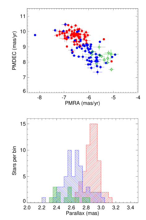
Figure 1: Proper motion diagram (top panel) and distribution of parallaxes (bottom panel) for the members of Gamma Vel A (red) and B (blue) from Jeffries et al. (2014) with RV membership probability $>0.75$. For comparison, we also plot the members of NGC 2547 B from Sacco et al. (2015, green diamonds and histogram).

2 Gaia analysis and results

The goal of this study is to perform a Gaia follow-up of the two populations discovered by Jeffries et al. (2014). For this reason, we start from the list of Gamma Velorum members published by these authors, which includes information on the radial velocity (RV) probability of belonging to the two populations (with $P_{\mathrm{RV,B}}=1-P_{\mathrm{RV,A}}$). These objects are distributed over an area of 0.9 sq. deg around the massive star, corresponding to $\sim\,6\times 6$ pc at the distance of Gamma Velorum. The list of members was crossmatched with the Gaia DR2 catalogue (Gaia Collaboration et al. 2018) in TOPCAT, using a 2″ radius to account for possible significant motions between the epoch of the 2MASS catalogue used in Jeffries et al. (2014) and Gaia DR2. We found Gaia counterparts for all objects, with separations $<0.4$″. We discarded from the sample 25 stars with astrometric excess noise $>1$ mas, which might indicate problems with the astrometric solution (e.g., Lindegren et al. 2018). Following Jeffries et al. (2014), we then extracted a subsample of 124 high-probability members of Gamma Vel A and B, by selecting stars with RV probability $>0.75$.

In Fig. 1 we plot the proper motion diagram and the parallax distribution for the high-probability members. The figure shows that there is a very clear separation between the two populations, although with some overlap, not only in the proper motions, as expected given the difference in kinematics found by Jeffries et al. (2014), but also in their parallaxes. In particular, the parallax distribution shows two well defined and separated peaks, implying that Gamma Vel A and B are located at different distances, with Gamma Vel A being closer than Gamma Vel B. There also appears to be a larger scatter in Gamma Vel B parallaxes and proper motions, while Gamma Vel A is more concentrated. In the same figure we also plot for comparison the members of NGC 2547 B derived by Sacco et al. (2015): these objects tend to have slightly higher values of $\mu_{\alpha*}$, but overlap completely with Gamma Vel B in both parallax and $\mu_{\delta}$, supporting the hypothesis that NGC 2547 B and Gamma Vel B are part of the same population. The small differences in parallax and proper motions might hint to possible gradients or substructures in population B, but our data do not allow to us to draw any conclusion.

Table 1: Result of the maximum-likelihood fit for the two populations

	Gamma Vel A	Gamma Vel B
$\varpi$ (mas)	$2.895\pm 0.008$	$2.608\pm 0.017$
$\sigma_{\varpi}$ (mas)	$0.038\pm 0.011$	$0.091\pm 0.016$
$\mu_{\alpha*}$ (mas/yr)	$-6.566\pm 0.043$	$-5.979\pm 0.074$
$\sigma_{\mu_{\alpha*}}$ (mas/yr)	$0.336\pm 0.032$	$0.490\pm 0.051$
$\mu_{\delta}$ (mas/yr)	$9.727\pm 0.047$	$8.514\pm 0.074$
$\sigma_{\mu_{\delta}}$ (mas/yr)	$0.341\pm 0.035$	$0.513\pm 0.056$
$f_{A}$	$0.599\pm 0.049$
$\ln L_{\mathrm{max}}$	$-83.8$

To quantify the differences between Gamma Vel A and B, we performed a maximum-likelihood fit of the 3D distribution of parallaxes and proper motions using two multivariate gaussian components, one for each population. Since the initial sample still contains a few clear residual outliers, to better constrain the fit we first excluded all objects falling at more than $5\sigma$ from the centroid of the total distribution. The fit was performed taking into account the full covariance matrix and the intrinsic dispersions of the parallaxes and proper motion components (see e.g. Lindegren et al. 2000); details are given in Appendix A. The resulting best-fit values are given in Table 1. Note that we obtain the same results, within the errors, also if we neglect the correlation coefficients, suggesting that correlations are not significant for this cluster.

For each star, we also derived astrometric membership probabilities $P_{\mathrm{Gaia,A}}$ and $P_{\mathrm{Gaia,B}}=1-P_{\mathrm{Gaia,A}}$, and selected the subsamples of Gamma Vel A and B members with $P_{\mathrm{Gaia,A}}>0.75$ (61 objects) and $P_{\mathrm{Gaia,B}}>0.75$ (46 objects), respectively. In Fig. 2 we compare the parallaxes and proper motions of these cleaned subsamples with the RVs from Jeffries et al. (2014). The figures show that, while Gamma Vel A is relatively compact and homogeneous, for Gamma Vel B there is a clear trend between the astrometric parameters and the RVs. Since the RVs are independent from the Gaia data, this suggests that the trend is real and not a consequence of correlations between the parameters. In particular, stars with lower RV tend to have larger parallax and total proper motion than those with higher RV. These results are not affected by the choice of the probability threshold used to select the cleaned sample: using a lower threshold would only slightly increase the scatter, leaving the trends unchanged.

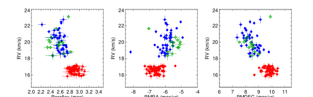
Figure 2: Comparison between the RVs from Jeffries et al. (2014) and the Gaia parallaxes and proper motions for stars with $P_{\mathrm{Gaia}}>0.75$. For comparison we also plot the NGC 2457 B members from Sacco et al. (2015). Symbols and colours are the same as in Fig. 1.

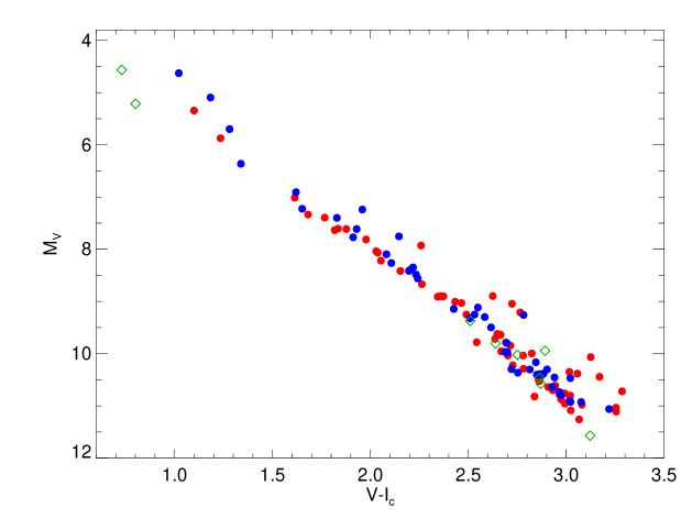
Figure 3: Absolute $V$ magnitude vs. $V-I_{\mathrm{c}}$ colour for the members of Gamma Vel A and B with $P_{\mathrm{Gaia}}>0.75$. $VI_{\mathrm{c}}$ photometry is from Jeffries et al. (2009). For comparison, we also plot the NGC 2547 B members with available $VI_{\mathrm{c}}$ photometry from Sacco et al. (2015), assuming the same average distance as Gamma Vel B. Colours are as in Fig. 1.

3 Discussion

3.1 The distance of Gamma Vel A and B

The main result of this study is the discovery that Gamma Vel A and B are located at different distances along the line of sight. In particular, we find parallaxes of $\varpi_{A}=2.895\pm 0.008$ mas for Gamma Vel A and $\varpi_{B}=2.608\pm 0.017$ mas for Gamma Vel B, with a difference of $\sim 0.29$ mas between the two populations. We caution that these results do not take into account possible systematic errors or correlations. Gaia DR2 parallaxes and proper motions can be affected by significant spatial correlations that can reach values of 0.04 mas and 0.07 mas/yr over scales $\la 1$ deg, as well as possible systematic effects that are expected to be $<0.1$ mas and $<0.1$ mas/yr (Lindegren et al. 2018; Luri et al. 2018). We performed a series of checks on the full Gaia sample over the region covered by our dataset, finding no evidence for significant spatial variations or correlations that could affect our results and produce the observed distributions and trends. While we cannot exclude systematic variations with respect to external regions, we can however be confident that the observed differences between the two populations are real.

Since the relative errors on parallaxes are below $\sim\,$10%, we can estimate the distances by a simple inversion of the parallaxes and calculate their uncertainties using a first order approximation (e.g. Bailer-Jones et al. 2018; Luri et al. 2018). Assuming conservatively a systematic error of $\pm 0.1$ mas, we obtain $d_{\mathrm{A}}=345.4^{+1.0+12.4}_{-1.0-11.5}$ pc and $d_{\mathrm{B}}=383.4^{+2.5+15.3}_{-2.5-14.2}$ pc for Gamma Vel A and B, respectively. Taking into account the average zero point in parallax of $\sim 0.03$ mas (Lindegren et al. 2018) would reduce both distances by $\sim 4$ pc. These results therefore show that Gamma Vel A is closer than Gamma Vel B by $\sim 38$ pc.

Our distance estimate for Gamma Vel A is consistent with the distance of $336^{+8}_{-7}$ pc derived for the massive star $\gamma^{2}$ Vel from interferometric observations (North et al. 2007) and with the revised Hipparcos distance of $343^{+39}_{-32}$ pc (van Leeuwen 2007). On the other hand, our distance estimate for Gamma Vel B is only marginally consistent with the value of $410\pm 12$ pc derived for the Vela OB2 association by de Zeeuw et al. (1999).

In Fig. 3 we plot the colour-magnitude diagram of the Gaia-selected sample after correcting for the distances to each population. The figure shows that the sequences of both single and binary stars are very clean for both Gamma Vel A and B, and that they overlap perfectly. By comparing linear fits in the colour-magnitude diagram with the Baraffe et al. (2015) isochrones for the two groups of secure members, it appears that any age difference between the populations is limited to about 3 Myr if the mean population age is 10 Myr, or double this if the mean age is 20 Myr (as suggested by Jeffries et al. 2017). However, the lithium depletion patterns in the two groups, which are distance-independent, suggest their ages are more similar than this (Jeffries et al. 2014). A more detailed analysis of the ages of the two populations will be presented in a forthcoming paper (Franciosini et al. in prep.).

3.2 The origin of the Gamma Velorum system

In the light of our results, we can now review the different hypothesis on the properties and the formation of the Gamma Velorum system.

From the parameters given in Table 1, we can derive the tangential velocity dispersions of the two populations, finding $\sim\,0.6$ km s^-1 and $\sim\,0.8$ km s^-1 for Gamma Vel A and B, respectively. These results are puzzling, since the values we find for Gamma Vel A and B are respectively larger and smaller than those obtained from the RVs ($0.34\pm 0.16$ km s^-1 and $1.60\pm 0.37$ km s^-1, respectively). In the case of Gamma Vel B, the observed dispersions could be different because on the plane of the sky we sample a region of the cluster which is smaller than what we sample along the line of sight, while the origin of the discrepancy for Gamma Vel A is not clear.

Figure 2 clearly shows an anti-correlation between radial velocities and parallaxes of Gamma Vel B. This signature is expected if the cluster is expanding as suggested by Sacco et al. (2015). They proposed that this expansion was triggered by the formation of $\gamma^{2}$ Vel, that expelled the residual gas keeping the cluster bound. However, as discussed in the previous section, the massive binary and Gamma Vel B are not at the same distance, therefore the dynamical status of the cluster and its evolution are unrelated with the massive binary. We can speculate that the cluster formed in an unbound state, or that its dispersion has been triggered by another massive star that evolved into a supernova. On the other hand, the distance of Gamma Vel A is consistent with $\gamma^{2}$ Vel, therefore, given that the massive binary is located at the cluster centre, we can conclude that it belongs to Gamma Vel A. It is still not clear why the ages of the cluster and of the central star are so different. Our results do not support the hypothesis that Gamma Vel B is part of the low-mass population of the Vela OB2 association, because the cluster appears to be located at a lower distance. However, a full study of the Vela region is required to address this issue.

Given their large separation, the two clusters are not merging as proposed by Mapelli et al. (2015), who assumed a much smaller distance between them ($\sim\,5$ pc) in their simulation of the dynamical interaction between the two systems. Furthermore, their relative velocities along the radial and tangential direction suggests that they did not merge in the past and will not do that in the future.

In conclusion our results suggests that Gamma Vel A and Gamma Vel B are two independent clusters seen along the same line of sight. Gamma Vel A is probably bound and formed the massive star $\gamma^{2}$ Vel, while Gamma Vel B is expanding.

4 Conclusions

In this paper we investigated the properties of the binary cluster Gamma Velorum using the Gaia DR2 astrometric parameters of cluster members pre-selected by spectroscopic observations. Our analysis led to the following main results:

1. We derived the distances of Gamma Vel A and B, finding that they are not cospatial, but Gamma Vel A is closer than Gamma Vel B by $\sim\,38$ pc. The separation between the two clusters indicates that they are not currently merging, while the comparison with the distance estimates for the massive binary $\gamma^{2}$ Vel suggests that this star belongs to Gamma Vel A.

2. We find that Gamma Vel B is expanding. However the origin of this expansion is not clear.

3. We confirm that the two clusters are kinematically separated and are moving apart. In particular, we find a shift in the tangential motion of Gamma Vel B with respect to Gamma Vel A of 0.6 and $-1.2$ mas yr^-1 ($\sim\,1$ and $-2$ km s^-1) along RA and DEC, respectively.

4. The colour-magnitude diagram corrected for the measured distance of each cluster indicates that the two populations are nearly coeval.

Appendix A Probability distribution of parallaxes and proper motions

To derive the mean parallaxes and proper motions of the two populations, we modeled the total probability distribution as the sum of two 3D multivariate gaussian components, one per population, given, for each population and each star, by:

$$L_{i}=\frac{1}{(2\pi)^{3/2}|\Sigma_{i}|^{-1/2}}\,\exp\left[-\frac{1}{2}(\@vec{x_{i}}-\@vec{x_{\circ}})^{T}\Sigma_{i}^{-1}(\@vec{x_{i}}-\@vec{x_{\circ}})\right]\,,$$ (1)

where

$$\@vec{x_{i}}-\@vec{x_{\circ}}=\left(\begin{array}[]{c}\varpi_{i}-\varpi_{\circ}\\ \mu_{\alpha*,i}-\mu_{\alpha*,\circ}\\ \mu_{\delta,i}-\mu_{\delta,\circ}\\ \end{array}\right)$$ (2)

and $\Sigma_{i}$ is the sum of the individual covariance matrix and the matrix of intrinsic dispersions:

$$\Sigma_{i}=\left(\begin{array}[]{ccc}\sigma_{\varpi,i}^{2}+\sigma_{\varpi,\circ}^{2}&\rho_{\varpi\mu_{\alpha*},i}\,\sigma_{\varpi,i}\,\sigma_{\mu_{\alpha*},i}&\rho_{\varpi\mu_{\delta},i}\,\sigma_{\varpi,i}\,\sigma_{\mu_{\delta},i}\\ \rho_{\varpi\mu_{\alpha*},i}\,\sigma_{\varpi,i}\,\sigma_{\mu_{\alpha*},i}&\sigma_{\mu_{\alpha*},i}^{2}+\sigma_{\mu_{\alpha*},\circ}^{2}&\rho_{\mu_{\alpha*}\mu_{\delta},i}\,\sigma_{\mu_{\alpha*},i}\,\sigma_{\mu_{\delta},i}\\ \rho_{\varpi\mu_{\delta},i}\,\sigma_{\varpi,i}\,\sigma_{\mu_{\delta},i}&\rho_{\mu_{\alpha*}\mu_{\delta},i}\,\sigma_{\mu_{\alpha*},i}\,\sigma_{\mu_{\delta},i}&\sigma_{\mu_{\delta},i}^{2}+\sigma_{\mu_{\delta},\circ}^{2}\\ \end{array}\right)$$ (3)