Self-calibrating vector atomic magnetometry through microwave polarization reconstruction

Abstract

Atomic magnetometry is one of the most sensitive ways to measure magnetic fields. We present a method for converting a naturally scalar atomic magnetometer into a vector magnetometer by exploiting the polarization dependence of hyperfine transitions in rubidium atoms. First, we fully determine the polarization ellipse of an applied microwave field using a self-calibrating method, i.e. a method in which the light-atom interaction provides everything required to know the field in an orthogonal laboratory frame. We then measure the direction of an applied static field using the polarization ellipse as a three-dimensional reference defined by Maxwell’s equations. Although demonstrated with trapped atoms, this technique could be applied to atomic vapors, or a variety of atom-like systems.

Sensitive magnetometers are increasingly important in both fundamental and technological applications. High accuracy and precision magnetometers are used for dark matter searches and aid in tests of fundamental symmetries. They enable applications ranging from navigation, timekeeping, and geophysical measurement to biological imaging. A wide array of application-specific requirements has yielded a wide array of magnetometry technologies, drawing on atomic vapors Bloom (1962); Budker and Romalis (2007), nitrogen-vacancy centers Rondin et al. (2014), nuclear magnetic resonance Gross et al. (2016), and superconducting quantum-interference devices Kleiner et al. (2004).

For many magnetometry applications measurement of the scalar field is sufficient, but also knowing the field’s full vector description can have important implications, in particular in geosensing Goetz et al. (1983); Reid et al. (1990); J. E. Lenz (1990) and the calibration of precision physics experiments Budker and Kimball (2013). However, mapping a magnetic field in three-dimensional space with a robust calibration is nontrivial, and presents distinct challenges in different platforms.

Superconducting quantum interference devices (SQUIDS) and Hall or fluxgate sensors are naturally sensitive to a field component perpendicular to, for example, a current loop. But multiple sensors must be used to measure the field in all three dimensions, and common problems are drifts or uncertainties in the relative directions of the axes F. Camps et al. (2009); Liu et al. (2014). Solid-state sensors such as nitrogen vacancy (NV) centers in diamond have emerged as a robust and broadband room-temperature platform for magnetic sensing and imaging. The inherent crystalline structure of NVs provides a natural reference for vector sensing that is actively being developed Alegre et al. (2007); Maertz et al. (2010); Wang et al. (2015); Lee et al. (2015); Münzhuber et al. (2017); Schloss et al. (2018).

The most precise magnetometers, which reach sensitivities beyond $\text{fT}/\sqrt{\text{Hz}}$, are atomic magnetometers that consist of many indistinguishable atoms in the vapor phase Kominis et al. (2003). However, as they are based on Larmor precession, they are scalar sensors, and there is no natural knob for breaking down the total field into components. In the most standard approach to an atomic vector magnetometer, vector addition of an applied static bias field and the field to be measured can be used to extract the unknown field direction Gravrand et al. (2001); Vershovskii et al. (2006); Seltzer and Romalis (2004). However, knowledge of the applied bias fields in a orthogonal laboratory frame is limited by the calibration of the external coil set used to apply the bias field. To avoid reliance upon mechanical construction tolerances for calibration, a number of ideas have been developed for atomic vector magnetometers, such as double-resonance magnetometers Weis et al. (2006); Pustelny et al. (2006); Ingleby et al. (2018), the use of electromagnetically-induced-transparency effects Cox et al. (2011); Lee et al. (1998), and orthogonal pump beams and effective fields of optical light Patton et al. (2014).

In this Letter, we introduce a spatial reference for vector atomic magnetometry based upon the three-dimensional structure of a microwave field. Our work draws on advances in another domain of magnetometry - that of microwave-field measurements and imaging based upon atomic spectroscopy Affolderbach et al. (2015); Kinoshita and Ishii (2016); Horsley and Treutlein (2016). In these techniques, a microwave field can be characterized through dependence of the atomic response on the polarization of the microwave radiation with respect to an applied quantization axis. In our work, we demonstrate a general algorithm for full reconstruction of a microwave polarization ellipse based upon atomic measurements. Importantly, we present how mapping the three-dimensional ellipse is self-calibrating: Systematics in the direction and strength of applied bias fields, e.g. non-orthogonal field orientations, can be located and corrected based upon the expected atomic response and electro-magnetic field structure.

Using the reconstructed microwave polarization ellipse as a fundamental reference, we demonstrate atomic vector magnetometry with a multi-level atom. We measure the strength and direction of an applied static magnetic field using only the microwave polarization information and the relative strength of atomic transitions, without the need for rotation of additional static fields. Our magnetometer can operate in either small field or with an applied reference field.

Our experiments take place using single trapped alkali atoms; while the sensitivity of the experiment undertaken with a few atoms is limited, it enables a proof-of-principle demonstration. In trapped atom experiments, developing knowledge of applied microwave polarization can be useful for optimization of atomic Rabi rates, characterization of effective magnetic fields in complex trapping potentials Kien et al. (2013); Thompson et al. (2013); Schneeweiss et al. (2014); Petersen et al. (2014); Goban et al. (2014); Kaufman (2015), and calibration of bias field directions for atomic clocks. However, in the context of atomic magnetometry, we envision our technique will be most relevant to hot-vapor cells, where one can measure magnetic fields with greater precision and versatility.

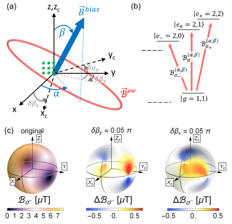
Figure 1: (a) Sketch of experimental setup. ⁸⁷Rb atoms (green) are trapped in nine optical tweezers and coherently manipulated using microwave radiation (red ellipse). The direction of a magnetic bias field $\vec{B}^{\text{bias}}$ (blue arrow) can be rotated in any direction given by Euler angles $\alpha$ and $\beta$ defined in the laboratory frame $(\vec{x},\vec{y},\vec{z})$. The bias coils form a slightly non-orthogonal coordinate frame $(\vec{x}_{\text{c}},\vec{y}_{\text{c}},\vec{z}_{\text{c}})$ with angles relative to the laboratory frame of $(\delta\beta_{x},\delta\alpha_{y},\delta\beta_{y})$. (b) Hyperfine transitions (red) between Zeeman-sublevels of ⁸⁷Rb. (c) [left panel] Strength of the $\mathcal{B}_{\sigma_{-}}$ component of a microwave field for all directions $(\alpha,\beta)$ of $\vec{B}^{\text{bias}}$ in the laboratory frame for an example polarization ellipse. [center and right panels] Differences in measured and predicted $\mathcal{B}_{\sigma_{-}}$ for the sample values of $\delta\beta_{x}$ and $\delta\beta_{y}$ are indicated.

We begin by describing our specific experimental setup and atomic multi-level structure, although the procedures we describe apply generally. We use single ⁸⁷Rb atoms loaded with $50\%$-probability into a regular $3\times 3$ array of $1.7$ $\mu$m-spaced optical tweezers [Fig. 1(a)] Kaufman (2015). We use four levels of ⁸⁷Rb: A ground-state $|g\rangle=|\text{F}=1,m_{\text{F}}=1\rangle$ and three excited hyperfine states $|e_{+}\rangle=|2,2\rangle$, $|e_{\pi}\rangle=|2,1\rangle$ and $|e_{-}\rangle=|2,0\rangle$ states.

We start the experiment by initializing the atoms in $|g\rangle$. During the experiment, we drive to the excited states using $\sigma_{\pm}$ and $\pi$-polarized light components of a $6.834$-GHz-microwave field ($\lambda\approx 44~{}\text{mm}$) of magnitude $|\vec{\mathcal{B}}^{\mu\text{w}}|_{\text{max}}\equiv\lVert\vec{\mathcal{B}}^{\mu\text{w}}\rVert\approx 7.8~{}\mu$T [Fig. 1(b)].

The transitions are split by a $300$-$\mu$T-strong static magnetic bias field $\vec{B}^{\text{bias}}$. The maximal splitting between the three transitions ($\sim 4.2$ MHz) is $<0.1\%$ of the microwave frequency, and hence spatial field differences are irrelevant when resonant with a transition. $\vec{B}^{\text{bias}}$ is controlled by three coil pairs in near-Helmholtz configurations that define a coil-frame $\mathcal{C}=(\vec{x}_{\text{c}},\vec{y}_{\text{c}},\vec{z}_{\text{c}})$ that importantly is not necessarily orthogonal. An orthonormal laboratory frame $\mathcal{L}=(\vec{x},\vec{y},\vec{z})$ is chosen s.t. $\vec{z}$ [Euler angles: $(\alpha,\beta)=(0,0)$] is oriented along $\vec{z}_{\text{c}}$, and $\vec{x}_{\text{c}}$ and $\vec{y}_{\text{c}}$ point in directions given by angles $(0,\pi/2+\delta\beta_{x})$, and $(\pi/2+\delta\alpha_{y},\pi/2+\delta\beta_{y})$, respectively [Fig. 1(a)].

We then determine the full polarization ellipse ($PE$) of the magnetic component of our microwave excitation field, expressed in $\mathcal{L}$ as:

$$\vec{\mathcal{B}}^{\mu\text{w}}=\sum_{\begin{subarray}{c}j\in\\ \{x,y,z\}\end{subarray}}\frac{1}{2}\mathcal{B}_{j}e^{-i(\phi_{j}+\omega t)}\vec{e}_{j}+\text{c.c.}$$ (1)

$\vec{\mathcal{B}}^{\mu\text{w}}$ traces the $PE$ determined by $5$ independent parameters: $3$ fields $(\mathcal{B}_{x},\mathcal{B}_{y},\mathcal{B}_{z})$ and two relative phases ($\phi_{x},\phi_{y}$), where $\phi_{z}=0$ without loss of generality Köpsell et al. (2017).

The quantization axis of our atoms is defined along $\vec{B}^{\text{bias}}$, and is always well-defined because $\lVert\vec{\mathcal{B}}^{\mu\text{w}}\rVert\ll|\vec{B}^{\text{bias}}|$. The microwave field amplitudes $\mathcal{B}_{\pm\sigma}$ and $\mathcal{B}_{\pi}$ that drive the $\Delta m_{\text{F}}=\pm 1$ and $\Delta m_{\text{F}}=0$ atomic transitions, respectively, are strongly dependent on the direction of $\vec{B}^{\text{bias}}$ and hence denoted as $\mathcal{B}_{i}^{(\alpha,\beta)}$ for $i\in(\sigma_{\pm},\pi)$ hereafter. The $\mathcal{B}_{i}^{(\alpha,\beta)}$ are related to the $5$ polarization-ellipse parameters and the direction of the bias field $(\alpha,\beta)$ by Köpsell et al. (2017):

$$\left(\mathcal{B}_{\pi}^{(\alpha,\beta)}\right)^{2}= \mathcal{B}_{z}^{2}\cos^{2}(\beta)$$

$$+\left(\mathcal{B}_{x}^{2}\cos^{2}(\alpha)+\mathcal{B}_{y}^{2}\sin^{2}(\alpha)\right)\sin^{2}(\beta)$$

$$+\mathcal{B}_{z}\mathcal{B}_{x}\sin(2\beta)\cos(\alpha)\cos(\phi_{x})$$

$$+\mathcal{B}_{z}\mathcal{B}_{y}\sin(2\beta)\sin(\alpha)\cos(\phi_{y})$$

$$+\mathcal{B}_{y}\mathcal{B}_{x}\sin(2\alpha)\sin^{2}(\beta)\cos(\phi_{x}-\phi_{y})$$ (2a)

$$\left(\mathcal{B}_{\pm\sigma}^{(\alpha,\beta)}\right)^{2}= \frac{1}{2}\left(\sum_{\begin{subarray}{c}j\in\\ \{x,y,z\}\end{subarray}}ˆ{}\mathcal{B}_{j}^{2}-\left[\mathcal{B}_{\pi}^{(\alpha,\beta)}\right]^{2}\right)$$

$$\pm\mathcal{B}_{x}\mathcal{B}_{y}\cos(\beta)\sin(\phi_{x}-\phi_{y})$$

$$\mp\mathcal{B}_{x}\mathcal{B}_{z}\sin(\alpha)\sin(\beta)\sin(\phi_{x})$$

$$\pm\mathcal{B}_{y}\mathcal{B}_{z}\cos(\alpha)\sin(\beta)\sin(\phi_{y}).$$ (2b)

Therefore, to recreate the full PE, $5$ independently chosen measurements of ($\mathcal{B}_{\pm\sigma}^{(\alpha,\beta)},\mathcal{B}_{\pi}^{(\alpha,\beta)}$) are enough to solve for the $5$ unknown ellipse parameters Köpsell et al. (2017). These measurements can either vary any combination of $(\alpha,\beta)$ or the atomic transition used.

We now discuss how we avoid systematic errors that may enter this procedure. First, we measure $\mathcal{B}_{i}^{(\alpha,\beta)}$ by choosing (pulsed) coherent population transfer T. Thiele and Regal ; Affolderbach et al. (2015); Horsley and Treutlein (2016); Fan et al. (2014); Thiele et al. (2015); Köpsell et al. (2017) to accurately extract $\mathcal{B}_{i}^{(\alpha,\beta)}$ from the corresponding (measured) Rabi frequency $\Omega_{i}^{(\alpha,\beta)}=\mu_{i}\mathcal{B}_{i}^{(\alpha,\beta)}\big{/}\hbar$. By referencing $\Omega_{i}^{(\alpha,\beta)}$ to a frequency standard, $\mathcal{B}_{i}^{(\alpha,\beta)}$ can be determined absolutely when calculating the magnetic transition dipole moments $\mu_{i}$ from basic assumptions T. Thiele and Regal .

However, systematic errors can also enter through discrepancies of the intended and actual applied direction ($\alpha,\beta$) of $\vec{B}^{\text{bias}}$. When performing any directional measurement with an atom(-like) system this is a general limitation which, so far, is typically addressed by relying on the quality of an externally-calibrated system. Let us label the potentially unknown systematic errors by $N^{\text{u}}$ parameters $\{U_{j}\}$, $j\in[1,N^{\text{u}}]$ - these will generally modify the value and direction of $\vec{B}^{\text{bias}}$. The $\{U_{j}\}$ can be self-calibrated by performing $\geq N^{\text{u}}$ additional measurements and then solving the system of $\geq N^{\text{u}}+5$ equations for $(\mathcal{B}_{x},\mathcal{B}_{y},\mathcal{B}_{z},\phi_{x},\phi_{y};\{U_{j}\})$.

In our experiment the parameters $\{U_{j}\}$ are: orientations of the coil pairs $(U_{1},U_{2},U_{3})=(\delta\beta_{x},\delta\beta_{y},\delta\alpha_{y})$ forming coil frame $\mathcal{C}$ [Fig. 1(a)], components of a (stray) magnetic field $(U_{4},U_{5},U_{6})=(B_{x}^{\text{s}},B_{y}^{\text{s}},B_{z}^{\text{s}})$ due to imperfect nulling of the ambient magnetic fields, and calibration errors in the applied bias field $(U_{7},U_{8},U_{9})=(|\vec{B}^{\text{bias}}|,\epsilon_{x},\epsilon_{y})$ when parameterizing $\vec{B}^{\text{bias}}=|\vec{B}^{\text{bias}}|(\epsilon_{x}b_{x},\epsilon_{y}b_{y},b_{z})$ using $\sum_{i\in(x,y,z)}b_{\text{i}}^{2}=1$ T. Thiele and Regal . For completeness, this set of parameters also includes the magnitude of $\vec{B}^{\text{bias}}$ that will be determined from Zeeman shifts, which is irrelevant for determining a PE, but defines a common scaling factor for all static fields. We therefore need $\geq 14$ measurements to self-calibrate our magnetometer and the bias-field strength.

Our self-calibration of the $\{U_{j}\}$ stems from the structure of the microwave light dictated by Maxwell’s equations. To illustrate the key idea, we consider two simple examples where either $U_{1}=\delta\beta_{x}$ or $U_{2}=\delta\beta_{y}$ are unknown. Assume all of the $N^{\text{u}}$ measurements are performed on the $\mathcal{B}_{\sigma_{-}}^{(\alpha,\beta)}$-component of an elliptically polarized microwave field. The expected values of $\mathcal{B}_{\sigma_{-}}$ for an example PE are shown in the lab frame $\mathcal{L}$ as a function of $(\alpha,\beta)$ [Fig. 1(c)]. If the coil frame deviates from the lab frame such that $(\beta_{x},\beta_{y})=(0,0.05\pi)$ the functional form of $\mathcal{B}_{\sigma_{-}}^{(\alpha,\beta)}=\mathcal{B}_{\sigma_{-}}(\alpha,\beta;\beta_{y})$ will deviate from the expectation in $\mathcal{L}$ with a specific pattern $\Delta\mathcal{B}_{\sigma_{-}}$ [center panel in Fig. 1(c)]. This field pattern cannot be reproduced by allowed microwave ellipses, and is distinctly connected to the unknown parameter. Importantly, a different pattern is associated with $(\beta_{x},\beta_{y})=(0.05\pi,0)$ [right panel in Fig. 1(c)]. Suitably chosen measurements on the sphere can hence lead to full differentiation and absolute characterization of the unknowns $\{U_{j}\}$.

To calibrate the $9$ $\{U_{j}\}$ in our experiment, we measure $\mathcal{B}_{\sigma_{-}}^{(\alpha,\beta)}$ (together with the Zeeman-shift of the $\sigma_{-}$-transition) for $28$ different directions $(\alpha,\beta)$ [black points in Fig. 2(a)]. Using quadratic minimization T. Thiele and Regal and Eq. (2b), these are enough measurements to determine $(\delta\beta_{x},\delta\alpha_{y},\delta\beta_{y})=(1.3\,\text{mrad},10.9\,\text{mrad},5.4\,\text{mrad}),~{}(B_{x}^{\text{s}},B_{y}^{\text{s}},B_{z}^{\text{s}})=(-6.05\,\mu\text{T},0.14\,\mu\text{T},-1.12\,\mu\text{T}),~{}|\vec{B}^{\text{bias}}|=302.0~{}\mu\text{T},$ $(\epsilon_{x},\epsilon_{y})=(1.001,0.989)$, and a polarization ellipse we refer to as $PE_{1}$: $(\mathcal{B}_{x},\mathcal{B}_{y},\mathcal{B}_{z},\phi_{x},\phi_{y})=(5.023(5)\,\mu\text{T},~{}5.757(4)\,\mu\text{T},~{}1.600(4)\,\mu\text{T},~{}-1.941(4),$ $-1.873(4))$ [red, dashed ellipse in Fig. 2(b)]. We cannot easily extract uncertainties for the $\{U_{j}\}$, but estimations have shown that we need to vary a $U_{j}$ by $\sim 20\%$ to change $PE_{1}$ by its uncertainty of $\lesssim 0.2\%$. Furthermore, the result is within expectation of experimentally-defined parameters in our setup T. Thiele and Regal ; for example the angles measured are consistent with machining tolerances of the coil mounts. The measured Zeeman shift allows us to determine the absolute value of $|\vec{B}^{\text{bias}}|$ that we find has a consistent dependence on $(\alpha,\beta)$ T. Thiele and Regal .

Figure 2(a) predicts $\mathcal{B}_{\sigma_{-}}^{(\alpha,\beta)}$ for all directions of $\vec{B}^{\text{bias}}$ using Eq. (2b), and could be used to optimize the atom-light coupling strength by choosing a suitable $\vec{B}^{\text{bias}}$. Furthermore, quantitative comparison with experiment provides a measure of how well $\{U_{j}\}$ and the ellipse parameters have been determined. For this, we investigate the relative errors $\Delta\mathcal{B}_{\sigma_{-},\text{rel.}}^{(\alpha,\beta)}$ of all measured $\mathcal{B}_{\sigma_{-}}^{(\alpha,\beta)}$ and their predicted values [see red histogram Fig. 2(c)]. Not surprisingly, we find that all $\Delta\mathcal{B}_{\sigma_{-},\text{rel.}}^{(\alpha,\beta)}$ are distributed around $0$, as they have been used to determine $PE_{1}$. The width of the distribution is consistent with the $\vec{\mathcal{B}}_{\sigma_{-}}^{(\alpha,\beta)}$ measurement uncertainty of $\sim 0.1\%$, and a microwave-amplitude drift of $\lesssim\pm 1\%$ occurring on timescales of several minutes T. Thiele and Regal . This drift could be stabilized in future experiments.

To elucidate experimentally self-calibration we determine a new polarization ellipse from a completely independent set of measurements: $\mathcal{B}_{\sigma_{+}}^{(0,0)},~{}\mathcal{B}_{\sigma_{-}}^{(0,0)},~{}\mathcal{B}_{\sigma_{+}}^{(0,\pi/2+\delta\beta_{x})},~{}\mathcal{B}_{\pi}^{(0,\pi/2+\delta\beta_{x})}$, and $\mathcal{B}_{\sigma_{-}}^{(0,\pi/2+\delta\beta_{x})}$, for which we rotate our bias field from the $\vec{z}_{\text{c}}$ to the $\vec{x}_{\text{c}}$ direction in the coil frame T. Thiele and Regal . Note, before we measured a single polarization for many directions, and now we measure all three polarization components for only two directions, i.e. we only rotate the bias field in a single plane once. Nonetheless, using Eqs. (2), we determine the microwave field in all three dimensions.

First, we assume (wrongly) that all $U_{j}=0$ (except $U_{7}=|\vec{B}^{\text{bias}}|=300~{}\mu$T), i.e. our coils are perfectly orthogonal, calibrated, and no stray magnetic fields are present. From this, we obtain $PE_{2}$: $(5.126(1)\,\mu\text{T},~{}5.786(1)\,\mu\text{T},~{}1.6537(7)\,\mu\text{T},~{}-1.970(3),$ $-1.910(2))$, depicted in black in Fig. 2(b). The shape and orientation of $PE_{2}$ agrees with $PE_{1}$ despite the different ways they were determined; but they are not identical. This is also captured in the corresponding distribution of $\Delta\mathcal{B}_{\sigma_{-},\text{rel.}}^{(\alpha,\beta)}$ of $PE_{2}$ [black histogram in Fig. 2(c)]. Its center is slightly offset from $0$, and indicates relative errors larger than $5\%$. These are larger than the slow drifts of our microwave source and the measurement uncertainties T. Thiele and Regal .

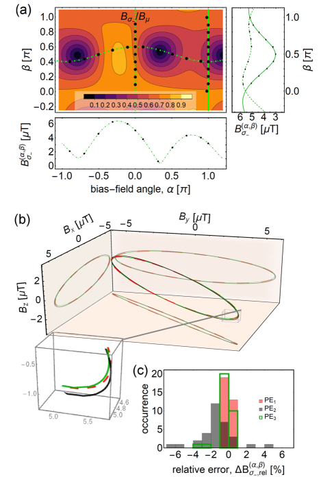
Figure 2: (a) (2D-plot) Predicted magnetic field component $\mathcal{B}_{\sigma_{-}}^{(\alpha,\beta)}$ using parameters from the polarization ellipse $PE_{1}$, as a function of the bias-field direction $(\alpha,\beta)$. (small panels) Measured magnetic microwave field component (black data) and predictions along the solid, dashed, and dot-dashed cuts in the 2D-plot, respectively. The measurement uncertainties are smaller than the datapoints. (b) Polarization ellipses $PE_{1}$(dashed, red), $PE_{2}$(black) and $PE_{3}$(green), respectively. $PE_{1}$ is the reference ellipse from the $30$ calibration measurements of $\mathcal{B}_{\sigma_{-}}^{(\alpha,\beta)}$ from panel (a). Comparison of ellipses $PE_{2}$ ($PE_{3}$) assess our protocol using $5$ of $6$ measurements T. Thiele and Regal without (with) taking into account calibrated $\{U_{j}\}$, see text. (c) Overlayed histograms of the relative errors $\Delta\mathcal{B}_{\sigma_{-},\text{rel.}}^{(\alpha,\beta)}$ of all polarization ellipses and for all measurements displayed in panel (a). The colorcoding is the same as for panel (b).

However, using the same $5$ measurements as for $PE_{2}$ now taking into account the correctly calibrated $\{U_{j}\}$, and a microwave drift correction of 1% T. Thiele and Regal , we obtain $PE_{3}$: $(5.070(1)\,\mu\text{T},~{}5.743(1)\,\mu\text{T},~{}1.6018(6)\,\mu\text{T},$ $-1.910(3),~{}-1.844(3))$ [green ellipse Fig. 2(b)]. This polarization ellipse predicts again the measurements correctly, i.e. the width of the $\Delta\mathcal{B}_{\sigma_{-},\text{rel.}}^{(\alpha,\beta)}$-distribution is consistent with our microwave drifts T. Thiele and Regal .

With the microwave field as a static, well-calibrated reference in the laboratory frame $\mathcal{L}$, we now use the atoms to vectorially resolve a set of $3$ intentionally applied static probe fields $\vec{B}^{\text{p}}$ in $\mathcal{L}$. The procedure: combine any scalar atomic measurement of $|\vec{B}^{\text{p}}|$ with two Rabi-rate measurements to solve for its orientation. Specifically, the $\sim 200~{}\mu$T-strong-probe magnetic fields $\vec{B}_{j}^{\text{p}}~{}[j=(x_{\text{c}},y_{\text{c}},z_{\text{c}})$] are sequentially applied along $\vec{x}_{\text{c}}$, $\vec{y}_{\text{c}}$, and $\vec{z}_{\text{c}}$, respectively, in addition to a reference field $\{|\vec{B}^{\text{ref}}|,\,(\alpha,\beta)^{\text{ref}}\}\approx\{300~{}\mu\text{T},(0.1\pi,0.6\pi)\}$. Then we measure the total magnetic bias field $\vec{B}_{j}^{\text{m}}=\vec{B}_{j}^{\text{p}}+\vec{B}^{\text{ref}}$ (and, for completeness $\vec{B}^{\text{ref}}$) and determine $\vec{B}_{j}^{\text{p}}$ by subtraction of $\vec{B}^{\text{ref}}$. The use of a reference field $\vec{B}^{\text{ref}}\neq 0$ is not necessary, but can be useful (see supplement T. Thiele and Regal ). All magnetic field magnitudes are found from the mean of the atomic Zeeman-shifts of all three available transitions. The directions $(\alpha,\beta)_{j}$ of $\vec{B}_{j}^{\text{m}}$ and $\vec{B}^{\text{ref}}$ are determined by measuring $\mathcal{B}_{\sigma_{-}}^{(\alpha,\beta)_{j}}$ and $\mathcal{B}_{\pi}^{(\alpha,\beta)_{j}}$ and then use Eq. (2) to solve for $(\alpha,\beta)_{j}$ via quadratic minimization T. Thiele and Regal . We also measure $\mathcal{B}_{\sigma_{+}}^{(\alpha,\beta)_{j}}$, but use this for keeping track of drifts in the amplitude of our applied microwave field.

We find $\{|\vec{B}^{\text{ref}}|,\,[\alpha,\beta]^{\text{ref}}\}=\{296.6(2)\,\mu\text{T},\,[0.103(1)\pi,$ $0.588(6)\pi]\}$ (brown lines). Sequential application of the $3$ probe fields $\vec{B}_{j}^{\text{p}}$ results in total measured fields $\{|\vec{B}_{j}^{\text{m}}|,$ $[\alpha,\beta]^{\text{m}}_{j}\}=\{476.1(8)\,\mu\text{T},~{}[0.0636(6)\pi,0.554(6)\pi]\}$, $\{301.5(3)\,\mu\text{T},$ $[0.108(2)\pi,0.396(4)\pi]\}$, and $\{399.2(5)\,\mu\text{T},$ $[0.260(1)\pi,0.577(2)\pi]\}$ [solid blue lines in Figure  3]. The multiple lines represent measurement uncertainties from bootstrapping the error with 200 trials. The difference in the uncertainties for these measurements is determined by the precision with which we measure the $\Omega_{i}^{(\alpha,\beta)}$, and by its transfer function to the field direction. This transfer function causes the uncertainties to be very asymmetric (aspect ratios up to $30$) and is ultimately linked to the choice of $\vec{B}^{\text{ref}}$ T. Thiele and Regal .

We determine the mean probe fields $\vec{B}_{j}^{\text{p}}=\vec{B}_{j}^{\text{m}}-\vec{B}^{\text{ref}}$ (black) as the difference between the blue ($\vec{B}_{j}^{\text{m}}$) and the brown ($\vec{B}^{\text{ref}}$) vectors. The probe fields that we expect (red lines) point in $\vec{x}_{\text{c}}$, $\vec{y}_{\text{c}}$ and $\vec{z}_{\text{c}}$-direction from $\vec{B}^{\text{ref}}$, and deviate from $\vec{B}_{j}^{\text{m}}-\vec{B}^{\text{ref}}$ by $16$ mrad, $79$ mrad and $23$ mrad, respectively. For the $\vec{y}_{\text{c}}$ and $\vec{z}_{\text{c}}$-direction, these values are just outside the confidence interval we expect based on the measurement uncertainties, but can be fully explained when including the slow drift of the microwave field strength reported earlier T. Thiele and Regal . Over the course of this set of measurements this drift was found to be $\leq\pm 0.5\%$ as inferred from all the measured magnitudes $7.841(8)~{}\mu\text{T},\,7.840(6)~{}\mu\text{T},\,7.789(5)~{}\mu\text{T}$, and $7.815(7)~{}\mu\text{T}$, respectively.

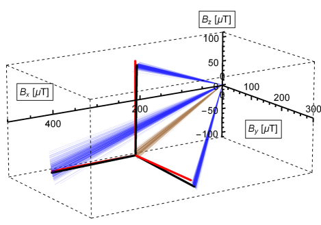
Figure 3: Vector magnetometry in an orthonormal laboratory frame $\mathcal{L}$: Targeted (red) applied magnetic field vectors $\vec{B}_{j}^{\text{p}}$, $j\in(x_{\text{c}},y_{\text{c}},z_{\text{c}})$, can be reconstructed (black) as the difference between all measured vectors $\vec{B}_{j}^{\text{m}}$ (dark blue lines) and an initially applied reference field $\vec{B}^{\text{ref}}$ (brown lines). The multiple lines for all displayed measured fields indicate the range of measurement errors, determined by bootstrapping the error with $200$ trials.

The magnetometer can operate with reference or without (reference-free) $\vec{B}^{\text{ref}}$. In contrast to the reference-free mode, in the reference-mode the uncertainty of $\vec{B}^{\text{ref}}$ adds to the uncertainty of our measurement of $\vec{B}_{j}^{\text{p}}$, but makes the measurement of $\vec{B}^{\text{p}}$ independent of common-mode background fields, a property specifically useful if $\vec{B}^{\text{p}}$ is time-dependent. Furthermore, $\vec{B}^{\text{ref}}\neq\vec{0}$ enables control over the precision of the vector magnetometer, and could even allow one to "squeeze" the measured variance in certain directions T. Thiele and Regal . Lastly, in reference-mode, one can avoid the complication of finding up to $4$ field solutions as a result of the measurements combined with the constraints of the trigonometric Eqs. (2) T. Thiele and Regal . In addition to this, we discuss in the supplement other strategies involving test-fields to determine the correct solution in the reference-free mode ($|\vec{B}^{\text{p}}|\gg|\vec{B}^{\text{ref}}|\approx 0$).

Looking forward, we envision reconstruction of the microwave polarization ellipse to be a general-purpose reference for not only magnetic fields, but other excitation fields (e.g optical fields or electric components). Further assessment is required to understand the potential for precision and sensitivity. Different measurement protocols will also need to be developed to transition these ideas to scalable and more-sensitive atomic vapor cells; coherent population transport was a robust way for us to measure microwave field strengths, but there are a variety of ways to determine the Rabi rates, e.g. by spectroscopic means. As with a variety of atomic sensors, this platform for vector magnetometry is compatible with futuristic quantum-enhancement, as established with cold atoms Degen et al. (2017); Muessel et al. (2014).

I Acknowledgments

We thank M. Knill for his help with bootstrapping analysis. We thank Svenja Knappe, Philip Treutlein, Ronald Walsworth, Adam Kaufman for helpful discussions, and Chris Kiehl for technical assistance. T.T. acknowledges funding from SNF under project number: P2EZP2_172208. We acknowledge funding from NSF Grant No. PHYS 1734006, ONR Grant No. N00014-17-1-2245, AFOSR-MURI Grant No. FA9550-16-1-0323, and the David and Lucile Packard Foundation. M. O. B. acknowledges support from an NDSEG Fellowship.

References

- Bloom (1962) Arnold L. Bloom, “Principles of operation of the rubidium vapor magnetometer,” Appl. Opt. 1, 61–68 (1962).
- Budker and Romalis (2007) Dmitry Budker and Michael Romalis, “Optical magnetometry,” Nature Physics 3, 227–234 (2007).
- Rondin et al. (2014) L. Rondin, J. P. Tetienne, T. Hingant, J. F. Roch, P. Maletinsky, and V Jacques, “Magnetometry with nitrogen-vacancy defects in diamond,” Reports on progress in physics 77, 056503 (2014).
- Gross et al. (2016) Simon Gross, Christoph Barmet, Benjamin E. Dietrich, David O. Brunner, Thomas Schmid, and Klaas P. Pruessmann, “Dynamic nuclear magnetic resonance field sensing with part-per-trillion resolution,” Nature communications 7, 13702 (2016).
- Kleiner et al. (2004) Reinhold Kleiner, Dieter Koelle, Frank Ludwig, and John Clarke, “Superconducting quantum interference devices: State of the art and applications,” Proceedings of the IEEE 92, 1534–1548 (2004).
- Goetz et al. (1983) Alexander F. H. Goetz, Barrett N. Rock, and Lawrence C. Rowan, “Remote sensing for exploration; an overview,” Economic Geology 78, 573–590 (1983).
- Reid et al. (1990) A. B. Reid, J. M. Allsop, H. Granser, A. J. Millett, and I. W. Somerton, “Magnetic interpretation in three dimensions using euler deconvolution,” Geophysics 55, 80–91 (1990).
- J. E. Lenz (1990) J. E. Lenz, “A review of magnetic sensors,” Proceedings of the IEEE 78, 973–989 (1990).
- Budker and Kimball (2013) D. Budker and D. F. J. Kimball, Optical Magnetometry (Cambridge University Press, Oxford, 2013).
- F. Camps et al. (2009) F. Camps, S. Harasse, and A. Monin, “Numerical calibration for 3-axis accelerometers and magnetometers,” in 2009 IEEE International Conference on Electro/Information Technology (2009) pp. 217–221.
- Liu et al. (2014) Yan Xia Liu, Xi Sheng Li, Xiao Juan Zhang, and Yi Bo Feng, “Novel calibration algorithm for a three-axis strapdown magnetometer,” Sensors 14, 8485–8504 (2014).
- Alegre et al. (2007) Thiago P. Mayer Alegre, Charles Santori, Gilberto Medeiros-Ribeiro, and Raymond G. Beausoleil, “Polarization-selective excitation of nitrogen vacancy centers in diamond,” Phys. Rev. B 76, 165205 (2007).
- Maertz et al. (2010) B. J. Maertz, A. P. Wijnheijmer, G. D. Fuchs, M. E. Nowakowski, and D. D. Awschalom, “Vector magnetic field microscopy using nitrogen vacancy centers in diamond,” Appl. Phys. Lett. 96, 092504 (2010).
- Wang et al. (2015) Pengfei Wang, Zhenheng Yuan, Pu Huang, Xing Rong, Mengqi Wang, Xiangkun Xu, Changkui Duan, Chenyong Ju, Fazhan Shi, and Jiangfeng Du, “High-resolution vector microwave magnetometry based on solid-state spins in diamond,” Nature communications 6, 6631 (2015).
- Lee et al. (2015) Sang-Yun Lee, Matthias Niethammer, and Jörg Wrachtrup, “Vector magnetometry based on s=3/2 electronic spins,” Physical Review B 92, 115201 (2015).
- Münzhuber et al. (2017) Franz Münzhuber, Johannes Kleinlein, Tobias Kiessling, and Laurens W. Molenkamp, “Polarization-assisted vector magnetometry in zero bias field with an ensemble of nitrogen-vacancy centers in diamond,” arXiv preprint arXiv:1701.01089 (2017).
- Schloss et al. (2018) Jennifer M. Schloss, John F. Barry, Matthew J. Turner, and Ronald L. Walsworth, “Simultaneous broadband vector magnetometry using solid-state spins,” arXiv:1803.03718 (2018).
- Kominis et al. (2003) I. K. Kominis, T. W. Kornack, J. C. Allred, and M. V. Romalis, “A subfemtotesla multichannel atomic magnetometer,” Nature 422, 596 (2003).
- Gravrand et al. (2001) O. Gravrand, A. Khokhlov, Le Mouël J. L., and Léger J. M., “On the calibration of a vectorial 4he pumped magnetometer,” Earth, planets and space 53, 949–958 (2001).
- Vershovskii et al. (2006) A. K. Vershovskii, M. V. Balabas, A. É. Ivanov, V. N. Kulyasov, A. S. Pazgalev, and E. B. Aleksandrov, “Fast three-component magnetometer-variometer based on a cesium sensor,” Technical Physics 51, 112–117 (2006).
- Seltzer and Romalis (2004) S. J. Seltzer and M. V. Romalis, “Unshielded three-axis vector operation of a spin-exchange-relaxation-free atomic magnetometer,” Applied physics letters 85, 4804–4806 (2004).
- Weis et al. (2006) Antoine Weis, Georg Bison, and Anatoly S Pazgalev, “Theory of double resonance magnetometers based on atomic alignment,” Physical Review A 74, 033401 (2006).
- Pustelny et al. (2006) S. Pustelny, W. Gawlik, S. M. Rochester, D. F. Jackson Kimball, V. V. Yashchuk, and D. Budker, “Nonlinear magneto-optical rotation with modulated light in tilted magnetic fields,” Phys. Rev. A 74, 063420 (2006).
- Ingleby et al. (2018) Stuart J. Ingleby, Carolyn O’ Dwyer, Paul F. Griffin, Aidan S. Arnold, and Erling Riis, “Vector magnetometry exploiting phase-geometry effects in a double-resonance alignment magnetometer,” arXiv preprint arXiv:1802.09273v1 (2018).
- Cox et al. (2011) Kevin Cox, Valery I. Yudin, Alexey V. Taichenachev, Irina Novikova, and Eugeniy E. Mikhailov, “Measurements of the magnetic field vector using multiple electromagnetically induced transparency resonances in rb vapor,” Phys. Rev. A 83, 015801 (2011).
- Lee et al. (1998) Hwang Lee, Michael Fleischhauer, and Marlan O. Scully, “Sensitive detection of magnetic fields including their orientation with a magnetometer based on atomic phase coherence,” Phys. Rev. A 58, 2587–2595 (1998).
- Patton et al. (2014) B. Patton, E. Zhivun, D. C. Hovde, and D. Budker, “All-optical vector atomic magnetometer,” Physical review letters 113, 013001 (2014).
- Affolderbach et al. (2015) C. Affolderbach, G. X. Du, T. Bandi, A. Horsley, P. Treutlein, and G. Mileti, “Imaging microwave and dc magnetic fields in a vapor-cell rb atomic clock,” IEEE Transactions on Instrumentation and Measurement 64, 3629–3637 (2015).
- Kinoshita and Ishii (2016) Moto Kinoshita and Masanori Ishii, “Measurement of microwave magnetic field in free space using the rabi frequency,” in Precision Electromagnetic Measurements (CPEM 2016), 2016 Conference on (IEEE, 2016) pp. 1–2.
- Horsley and Treutlein (2016) Andrew Horsley and Philipp Treutlein, “Frequency-tunable microwave field detection in an atomic vapor cell,” Applied Physics Letters 108, 211102 (2016).
- Kien et al. (2013) Fam Le Kien, Philipp Schneeweiss, and Arno Rauschenbeutel, “Dynamical polarizability of atoms in arbitrary light fields: general theory and application to cesium,” Eur. Phys. J. D 67, 92 (2013).
- Thompson et al. (2013) J. D. Thompson, T. G. Tiecke, A. S. Zibrov, V. Vuletic, and M. D. Lukin, “Coherence and Raman sideband cooling of a single atom in an optical tweezer,” Phys. Rev. Lett. 110, 133001 (2013).
- Schneeweiss et al. (2014) Philipp Schneeweiss, Fam Le Kien, and Arno Rauschenbeutel, “Nanofiber-based atom trap created by combining fictitious and real magnetic fields,” New Journal of Physics 16, 013014 (2014).
- Petersen et al. (2014) Jan Petersen, Jürgen Volz, and Arno Rauschenbeutel, “Chiral nanophotonic waveguide interface based on spin-orbit interaction of light,” Science 346, 67–71 (2014).
- Goban et al. (2014) A. Goban, C.-L. Hung, S.-P Yu, J.D. Hood, J.A. Muniz, J.H. Lee, M.J. Martin, A.C. McClung, K.S. Choi, D.E. Chang, O. Painter, and H. J. Kimble, “Atom-Light Interactions in Photonic Crystals,” Nat. Commun. 5, 3808 (2014).
- Kaufman (2015) A. M. Kaufman, Laser-cooling atoms to indistinguishability: Atomic Hong-Ou-Mandel interference and entanglement through spin exchange, Ph.D. thesis, University of Colorado at Boulder (2015).
- Köpsell et al. (2017) J. Köpsell, T. Thiele, J. Deiglmayr, A. Wallraff, and F. Merkt, “Measuring the polarization of electromagnetic fields using rabi-rate measurements with spatial resolution: experiment and theory,” Phys. Rev. A (2017).
- (38) M. O. Brown T. Thiele, Y. Lin and C. Regal, “Supplementary information for …” .
- Fan et al. (2014) H. Q. Fan, S. Kumar, R. Daschner, H. Kübler, and J. P. Shaffer, “Sub-wavelength microwave electric field imaging using rydberg atoms inside atomic vapor cells,” arXiv:1403.3596 (2014).
- Thiele et al. (2015) T. Thiele, J. Deiglmayr, M. Stammeier, J.-A. Agner, H. Schmutz, F. Merkt, and A. Wallraff, “Imaging electric fields in the vicinity of cryogenic surfaces using rydberg atoms,” Phys.Rev. A (2015).
- Degen et al. (2017) C. L. Degen, F. Reinhard, and P. Cappellaro, “Quantum sensing,” Rev. Mod. Phys. 89, 035002 (2017).
- Muessel et al. (2014) W. Muessel, H. Strobel, D. Linnemann, D. B. Hume, and M. K. Oberthaler, “Scalable spin squeezing for quantum-enhanced magnetometry with bose-einstein condensates,” Phys. Rev. Lett. 113, 103004 (2014).