Coordinating the Motion of Labeled Discs with Optimality Guarantees under Extreme Density

Abstract

We push the limit in planning collision-free motions for routing uniform labeled discs in two dimensions. First, from a theoretical perspective, we show that the constant-factor time-optimal routing of labeled discs can be achieved using a polynomial-time algorithm with robot density over $50\%$ in the limit (i.e., over half of the workspace may be occupied by the discs). Second, from a more practical standpoint, we provide a high performance algorithm that computes near-optimal (e.g., $1.x$) solutions under the same density setting.

1 Introduction

The routing of rigid bodies (e.g., mobile robots) to desired destinations under dense settings (i.e., many rigid bodies in a confined workspace) is a challenging yet high utility task. On the side of computational complexity, when it comes to feasibility (i.e., finding collision-free paths for moving the bodies without considering path optimality), it is well known that coordinating the motion of translating rectangles is PSPACE-hard [1] whereas planning for moving labeled discs of variable sizes is strongly NP-hard in simple polygons [2]. More recently, it is further established that PSPACE-hardness extends to the unlabeled case as well [3]. Since computing an arbitrary solution is already difficult under these circumstances, finding optimal paths (e.g., minimizing the task completion time or the distances traveled by the bodies) are at least equally hard. Taking a closer look at proof constructions in [1, 3, 2], one readily observes that the computational difficulty increases as the bodies are packed more tightly in the workspace. On the other hand, in many multi-robot applications, it is desirable to have the capacity to have many robots efficiently and (near-)optimally navigate closely among each other, e.g., in automated warehouses [4, 5]. Provided that per-robot efficiency and safety are not compromised, having higher robot density directly results in space and energy savings, thus enhancing productivity.

As a difficult but intriguing geometric problem, the optimal routing of rigid bodies has received much attention in many research fields, particularly robotics. While earlier research in the area tends to focus on the structural properties and complete (though not necessarily scalable) algorithmic strategies [6, 7, 8, 9, 10], more recent studies have generally attempted to provide efficient and scalable algorithms with either provable optimality guarantees or impressive empirical results, or both. For the unlabeled case, a polynomial-time algorithm from [11] computes trajectories for uniform discs which minimizes the maximal path length traveled by any disc. The completeness of the algorithm depends on some clearance assumptions between the discs and between a disc and the environment. In [12], a polynomial-time complete algorithm algorithm is proposed also for unlabeled discs that optimizes the total travel distance, with a more natural clearance assumption as compared to [11]. The clearance assumption (among others, the distance between two unit discs is at least $4$) translates to a maximum density of about $23\%$, i.e., the discs may occupy at most $23\%$ of the available free space. For the labeled case, under similar clearance settings, an integer linear programming (ILP) based method is provided in [13] for minimizing solution makespan. Though without polynomial running time guarantee, the algorithm is complete and appears to performs well in practice. Complete polynomial-time algorithms also exist that do not require any clearance in the start and goal configurations [14]. However, the supported density is actually lower in this case as the algorithm needs to expand the start and goal configurations so that the clearance conditions in [13] is satisfied.

In this work, we study the problem of optimally routing labeled uniform unit discs in a bounded continuous two dimensional workspace. As the main result, we provide a complete, deterministic, and polynomial-time algorithm that allow up to more than half of the workspace to be occupied by the discs while simultaneously ensuring $O(1)$ (i.e., constant-factor) time optimality of the computed paths. We also provide a practical and fast algorithm for the same setting without the polynomial running time guarantee. More concretely, our study brings the following contributions: (i) We show that when the distance between the centers of any two labeled unit discs is more than $\frac{8}{3}$, the continuous problem can be transformed into a multi-robot routing problem on a triangular grid graph with minimal optimality loss. A separation of $\frac{8}{3}$ implies a maximum density of over $50\%$. (ii) We develop a low polynomial-time constant-factor time-optimal algorithm for routing discs on a triangular grid with the constraint that no two discs may travel on the same triangle concurrently. (iii) We develop a fast and novel integer linear programming (ILP) based algorithm that computes time-optimal routing plans for the triangular grid-based multi-robot routing problem. Combining (i) and (ii) yields the $O(1)$ time-optimal algorithm while combining (i) and (iii) results in the more practical and highly optimal algorithm. In addition, the $\frac{8}{3}$ separation proof employs both geometric arguments and computation-based verification, which may be of independent interest.

Our work leans on graph-theoretic methods for multi-robot routing, e.g., [15, 16, 17, 18, 19, 20, 21]. In particular, our constant-factor time-optimal routing algorithm for the triangular grids adapts from a powerful routing method for rectangular grid in [16] that actually works for arbitrary dimensions. However, while the method from [16] comes with strong theoretical guarantee and runs in low polynomial time, the produced paths are not ideal due to the large constant factor. This prompts us to also look at more practical algorithms and we choose to build on the fast ILP-based method from [21], which allows us to properly encode the additional constraints induced by the triangular grid, i.e., no two discs may simultaneously travel along any triangle.

Organization. The rest of the paper is organized as follows. We provide a formal statement of the routing problem and its initial treatment in Section 2. In Section 3, we show how the problem may be transformed into a discrete one on a special triangular grid. Then, in Section 4 and Section 5, we present a polynomial time algorithm with $O(1)$-optimality guarantee and a fast algorithm that computes highly optimal solutions, respectively. We conclude in Section 6.

2 Preliminaries

2.1 Labeled Disc Routing: Problem Statement

Let $\mathcal{W}$ denote a closed and bounded $w\times h$ rectangular region. For technical convenience, we assume $w=4n_{1}+2$ and $h=\frac{4}{\sqrt{3}}n_{2}+2$ for integers $n_{1}\geq 2$ and $n_{2}\geq 3$. There are $n$ labeled unit discs residing in $\mathcal{W}$. Also for technical reasons, we assume that the discs are open, i.e., two discs are not in collision when their centers are exactly distance two apart. These discs may move in any direction with an instantaneous velocity $v$ satisfying $|v|\in[0,1]$. Let $\mathcal{C}_{f}\subset\mathbb{R}^{2}$ denote the free configuration space for a single robot in $\mathcal{W}$. The centers of the $n$ discs are initially located at $\mathcal{S}=\{s_{1},\ldots,s_{n}\}\subset\mathcal{C}_{f}$, with goals $\mathcal{G}=\{g_{1},\ldots,g_{n}\}\subset\mathcal{C}_{f}$. For all $1\leq i\leq n$, a disc labeled $i$ initially located at $s_{i}$ must move to $g_{i}$.

Beside planning collision-free paths, we want to optimize the resulting path quality by minimizing the global task completion time, also commonly known as the makespan. Let $P=\{p_{1},\ldots,p_{n}\}$ denote a set of feasible paths with each $p_{i}$ a continuous function, defined as

$$p_{i}:[0,t_{f}]\to C_{f},p_{i}(0)=s_{i},p_{i}(t_{f})=g_{i},$$ (1)

the makespan objective seeks a solution that minimizes $t_{f}$, i.e., let $\mathcal{P}$ denote the set of all feasible solution path sets, the task is to find a set $P$ with $t_{f}(P)$ approaching the optimal solution

$$t_{min}:=\min_{P\in\mathcal{P}}t_{f}(P).$$ (2)

Positive separation between the labeled discs is necessary to render the problem feasible (regardless of optimality). In this work, we require the following clearance condition between a pair of $s_{i}$ and $s_{j}$ and a pair of $g_{i}$ and $g_{j}$:

$$\forall 1\leq i,j\leq n,\quad\parallel s_{i}-s_{j}\parallel>\frac{8}{3},\>\>\parallel g_{i}-g_{j}\parallel>\frac{8}{3}.$$ (3)

For notational convenience, we denote the problem address in this work as the Optimal Labeled Disc Routing problem (OLDR). By assumption (3) and assuming that the unit discs occupy the vertices of a regular triangular grid, the discs may occupy $({\frac{1}{2}\pi*1^{2}})/(\frac{1}{2}\frac{8}{3}*\frac{4}{\sqrt{3}})\approx 51\%$ of the free space in the limit (to see that this is the case, we note that each equilateral triangle with side length $\frac{8}{3}$ contains half of a unit disc; each corner of the triangle contains $\frac{1}{6}$ of a disc).

2.2 Workspace Discretization

Similar to [6, 9, 10, 13], we approach OLDR through first discretizing the problem, starting by embedding a discrete graph within $\mathcal{W}$. The assumption of $w=4n_{1}+2$ and $h=\frac{4}{\sqrt{3}}n_{2}+2$ on the workspace dimensions allows the embedding of a triangular grid with side length of $\frac{4}{\sqrt{3}}$ in $\mathcal{W}$ such that the grid has $2n_{1}$ columns and about $n_{2}$ (zigzagging) rows of equilateral triangles, and a clearance of $1$ from $\partial\mathcal{W}$. An example is provided in Fig. 1.

\begin{overpic}[width=346.89621pt,tics=5]{figures/tri-grid-example-eps-converted-to.pdf} \put(48.0,40.5){{\small$w$}} \put(79.6,18.0){{\small$h$}} \put(23.0,4.0){{\small$\mathcal{W}$}} \end{overpic}

Figure 1: An example of a workspace $\mathcal{W}$ with $w=14$ and $h=3\frac{4}{\sqrt{3}}+2$, i.e., $n_{1}=3$ and $n_{2}=3$. The embedded triangular grid is at least distance $1$ from the boundary of $\mathcal{W}$. The grid has $6$ columns and $2+$ zigzagging rows.

Throughout the paper, we denote the underlying graph of the triangular grid as $G$. Henceforth, we assume such a triangular grid $G$ for a given workspace $\mathcal{W}$. The choice of the side length of $\frac{4}{\sqrt{3}}$ for the triangular grid ensures that two unit discs located on adjacent vertices of $G$ may move simultaneously on $G$ without collision when the angle formed by the two traveled edges is not sharp (Fig. 2).

\begin{overpic}[width=346.89621pt,tics=5]{figures/hex-tri-collision-eps-converted-to.pdf} \end{overpic}

Figure 2: On a triangular grid with a side length of $\frac{4}{\sqrt{3}}$, two unit discs, initially residing on two adjacent vertices of the grid, may travel concurrently on the grid without collision when the two trajectories do not form a sharp angle. In the figure, the two cyan discs may travel as indicated without incurring collision. On the other hand, the red discs will collide if they follow the indicated travel directions.

We note that $w\geq 10$ and $h\geq 3\frac{4}{\sqrt{3}}+2$ are needed for our algorithm to have completeness and optimality guarantees. For smaller $w$ or $h$, an instance may not be solvable. On the other hand, the discrete increment assumption on $w$ and $h$ are for technical convenience and are not strictly necessary. Without these discrete increments assumptions, we will need additional (and more complex) clearance assumptions between the discs and $\partial\mathcal{W}$, which does not affect the $51\%$ density bound since $\partial\mathcal{W}$ contributes $\Theta(w+h)$ to the area of $\mathcal{W}$ which is $wh$. The ratio is $\Theta(\frac{w+h}{wh})$ which goes to zero as both $w$ and $h$ increase. We also mention that, although this study only considers bounded rectangular workspace without static obstacles within the workspace, our results can be directly combined with [13] to support static obstacles.

3 Translating Continuous Problems to Discrete Problems with Minimal Penalty on Optimality

A key insight enabling this work is that, under the separation condition (3), a continuous OLDR can be translated into a discrete one with little optimality penalty. The algorithm for achieving this is relatively simple. For a given $\mathcal{W}$ and the corresponding $G=(V,E)$ embedded in $\mathcal{W}$, for each $s_{i}\in\mathcal{S}$, let $v_{i}^{s}\in V$ be a vertex of $G$ that is closest to $s_{i}$ (if there are more than one such $v_{i}^{s}$, pick an arbitrary candidate). After all $v_{i}^{s}$'s (let $V_{\mathcal{S}}=\{v_{i}^{s}\}$) are identified for $1\leq i\leq n$, let $d_{\max}=\max_{i}\parallel v_{i}^{s}-s_{i}\parallel$. Note that $d_{\max}\leq\frac{4}{3}$. We then let the labeled discs at $s_{i}$ move in a straight line to the corresponding $v_{i}^{s}$ at a constant speed given by $\frac{\parallel v_{i}^{s}-s_{i}\parallel}{d_{\max}}$, which means that for all $1\leq i\leq n$, disc $i$ will reach $v_{i}^{s}$ in exactly one unit of time. The same procedure is then applied to $\mathcal{G}$ to obtain $V_{\mathcal{G}}=\{v_{i}^{g}\}$. The discrete OLDR is fully defined by $(G,V_{\mathcal{S}},V_{\mathcal{G}})$. We denote the algorithm as DiscretizeOLDR. Fig. 3 illustrates the assignment of a few unit discs to vertices of the triangular grid.

\begin{overpic}[width=346.89621pt,tics=5]{figures/to-discrete-eps-converted-to.pdf} \end{overpic}

Figure 3: An illustration of assigning a few unit discs to vertices of the triangular grid.

Because it takes a constant amount computational effort to deal with one disc, DiscretizeOLDR runs in linear time, i.e.,

Proposition 1.

DiscretizeOLDR has a running time of $O(n)$.

The rest of this section is devoted to showing that DiscretizeOLDR is collision-free and incurs little penalty on time optimality. We only need to show this for translating $\mathcal{S}$ to $V_{\mathcal{S}}$; translating $\mathcal{G}$ to $V_{\mathcal{G}}$ is a symmetric operation. We first make the straightforward observation that DiscretizeOLDR adds a makespan penalty of up to four because translating $\mathcal{S}$ to $V_{\mathcal{S}}$ takes exactly one unit of time. Same holds for translating $\mathcal{G}$ to $V_{\mathcal{G}}$.

Proposition 2.

DiscretizeOLDR incurs a makespan penalty of up to four.

We then show DiscretizeOLDR assigns a unique $v_{i}^{s}\in V$ for a given $s_{i}\in S$.

Lemma 3.

DiscretizeOLDR assign a unique $v_{i}^{s}\in V$ for an $s_{i}\in S$.

Proof.

Each equilateral triangle in $G$ has a side length of $\frac{4}{\sqrt{3}}$, which means that the distance from the center of a triangle to its vertices is $\frac{4}{3}$. Therefore, for any $s_{i}\in S$, it must be at most of distance $\frac{4}{3}$ to at least one vertex of $G$. Let this vertex be $v_{i}^{s}$. Now given any other $s_{j}\in\mathcal{S}$, assume DiscretizeOLDR assigns to it $v_{j}^{s}$. We argue that $v_{i}^{s}\neq v_{j}^{s}$ because otherwise

$$\frac{4}{3}+\frac{4}{3}\geq\parallel v_{i}-v_{i}^{s}\parallel+\parallel v_{j}-v_{j}^{s}\parallel=\parallel v_{i}-v_{i}^{s}\parallel+\parallel v_{j}-v_{i}^{s}\parallel\geq\parallel v_{i}-v_{j}\parallel>\frac{8}{3},$$

which is a contradiction. Here, the first $\geq$ holds because $\parallel v_{i}-v_{i}^{s}\parallel\leq\frac{4}{3}$ and $\parallel v_{j}-v_{j}^{s}\parallel\leq\frac{4}{3}$ by DiscretizeOLDR; the second $\geq$ is due to the triangle inequality. The $>$ is due to assumption  (3).  ∎∎

Next, we establish that DiscretizeOLDR is collision-free. For the proof, we use geometric arguments assisted with computation-based case analysis.

Theorem 4.

DiscretizeOLDR guarantees collision-free motion of the discs.

Proof.

We fix a vertex $v\in V$ of the triangular grid $G$. By Lemma 3, at most one $s_{i}\in\mathcal{S}$ may be matched with $v$, in which case $v$ becomes $v_{i}^{s}$. If this is the case, then $s_{i}$ must be located within one of the six equilateral triangles surrounding $v$. Assume with out loss of generality that $s_{i}$ belongs to an equilateral triangle $\triangle uvw$ as shown in Fig. 4(a). The rules of DiscretizeOLDR further imply that $s_{i}$ must fall within one (e.g., the orange shaded triangle in Fig 4 (a)) of the six triangles belonging to $\triangle uvw$ that are formed by the three bisectors of $\triangle uvw$. Let this triangle be $\triangle vox$. Now, let $s_{j}\neq s_{i}$ be the center of a labeled disc $j$; assume that disc $j$ go to some $v_{j}^{s}\in V$. By symmetry, if we can show that disc $i$ with $s_{i}\in\triangle vox$ and an arbitrary disc $j$ with $\parallel s_{i}-s_{j}\parallel>\frac{8}{3}$ will not collide with each other as disc $i$ and disc $j$ move along $s_{i}v_{i}^{s}$ and $s_{j}v_{j}^{s}$, respectively, then DiscretizeOLDR is a collision-free procedure.

\begin{overpic}[width=346.89621pt,tics=5]{figures/collision-free-eps-converted-to.pdf} \put(-3.0,22.0){{\small$u$}} \put(32.0,41.0){{\small$w$}} \put(22.0,3.5){{\small$v(v_{i}^{s})$}} \put(17.0,24.0){{\small$o$}} \put(32.0,22.0){{\small$x$}} \put(26.0,18.0){{\small$s_{i}$}} \put(73.5,18.5){{\small$s_{i}$}} \put(75.5,11.0){{\small$v_{i}^{s}$}} \put(90.5,15.0){{\small$s_{j}$}} \put(85.0,18.5){{\small$v_{j}^{s}$}} \put(18.0,-4.0){{\small(a)}} \put(72.5,-4.0){{\small(b)}} \end{overpic}

Figure 4: (a) By symmetry, for an $s_{i}\in\mathcal{S}$ to be moved to some $v=v_{i}^{s}$, we only need to consider the region $\triangle vox$, which is $\frac{1}{12}$-th of all possible places where $s_{i}$ may appear. (b) For a fixed $s_{i}$, we only need to consider $s_{j}$ that is of exactly $\frac{8}{3}$ distance from it.

We then make the observation that, if disc $i$ and disc $j$ collide as we align their centers to vertices of the triangular grid, at some point, the distance between their centers must be exactly $\frac{8}{3}$ before they may collide (when their centers are of distance less than $2$). Following this reasoning, instead of showing a disc $j$ with $\parallel s_{i}-s_{j}\parallel>\frac{8}{3}$ will not collide with disc $i$, it suffices to show the same only for $\parallel s_{i}-s_{j}\parallel=\frac{8}{3}$. That is, it is sufficient to show that, for any $s_{i}\in\triangle vox$ and any $s_{j}$ on a circle of radius $\frac{8}{3}$ centered at $s_{i}$, disc $i$ and disc $j$ will not collide as $s_{i}$ and $s_{j}$ move to $v_{i}^{s}$ and $v_{j}^{s}$, respectively, according to the rules specified by DiscretizeOLDR (see Fig. 4(b) for an illustration).

To proceed from here, one may attempt direct case-by-case geometric analysis, which appears be quite tedious. We instead opt for a more direct computer assisted proof as follows. We first partition $\triangle vox$ using axis-aligned square grids with side length $\varepsilon$; $\varepsilon$ is some parameter to be determined through computation. For each of the resulting $\varepsilon\times\varepsilon$ square region (a small green square in Fig. 5), we assume that $s_{i}$ is at its center. For each fixed $s_{i}$, an annulus centered at $s_{i}$ with inner radius $\frac{8}{3}-\frac{\sqrt{2}\varepsilon}{2}$ and outer radius $\frac{8}{3}+\frac{\sqrt{2}\varepsilon}{2}$ is obtained (part of which is illustrated as in Fig. 5). Given this construction, for any potential $s_{i}^{\prime}$ in a fixed $\varepsilon\times\varepsilon$ square, a circle of radius $\frac{8}{3}$ around it falls within the annulus.

We then divide the outer perimeter of the annulus into arcs of length no more than $\sqrt{2}\varepsilon$. For each piece, we obtain a roughly square region with side length $\sqrt{2}\varepsilon$ on the annulus, one of which is shown as the red square in Fig. 5. We take the center of the square as $s_{j}$. We then fix $v_{j}^{s}$ accordingly (note that it may be the case that $v_{j}^{s}$ is not unique for the square that bounds a piece of arc, in which case we will attempt all potentially valid $v_{j}^{s}$'s).

\begin{overpic}[width=346.89621pt,tics=5]{figures/discretize-square-grid-eps-converted-to.pdf} \put(31.0,33.2){{\small$s_{i}$}} \put(37.0,19.2){{\small$v_{i}^{s}$}} \put(73.0,18.0){{\small$s_{j}$}} \put(64.0,40.0){{\small$v_{j}^{s}$}} \end{overpic}

Figure 5: Illustration of picking a pair of $s_{i}$ and $s_{j}$ for a computer based proof.

For each fixed set of $s_{i},v_{i}^{s},s_{j}$, and $v_{j}^{s}$, following the rules of DiscretizeOLDR, we may (analytically) compute the shortest distance between the centers of disc $i$ and disc $j$ as disc $i$ is moved from $s_{i}$ to $v_{i}^{s}$ while disc $j$ is moved from $s_{j}$ to $v_{j}^{s}$. Let the trajectory followed by the two centers in this case be $\tau_{i}(t)$ and $\tau_{j}(t)$, respectively, with $0\leq t\leq 1$ (as guaranteed by DiscretizeOLDR), we may express the distance (for fixed $\varepsilon$, $s_{i},v_{i}^{s},s_{j}$, and $v_{j}^{s}$) as $\delta_{\varepsilon}(s_{i},s_{j})=\min_{t}\parallel\tau_{i}(t)-\tau_{j}(t)\parallel$. For any $s_{i}^{\prime}$ that falls in the same $\varepsilon\times\varepsilon$ box as $s_{i}$, if disc $i$ is initially located at $s_{i}^{\prime}$, let it follow a trajectory $\tau_{i}^{\prime}(t)$ to $v_{i}^{s}$. We observe that $\parallel\tau_{i}(t)-\tau_{i}^{\prime}(t)\parallel\leq\varepsilon$. This holds because as the center of disc $i$ moves from anywhere within the $\varepsilon\times\varepsilon$ box to $v_{i}^{s}$, $\parallel\tau_{i}(t)-\tau_{i}^{\prime}(t)\parallel$ continuously decreases until it reaches to zero at $v_{i}^{s}$, which is the same for both $s_{i}$ and $s_{i}^{\prime}$. Therefore, the initial uncertainty is the largest, which is no more than $\varepsilon$ because $\parallel s_{i}-s_{i}^{\prime}\parallel\leq\frac{\sqrt{2}\varepsilon}{2}$. The same argument applies to disc $j$, i.e., $\parallel\tau_{j}(t)-\tau_{j}^{\prime}(t)\parallel\leq\varepsilon$. Therefore, we have

$$\delta_{\varepsilon}(s_{i},s_{j}) =\min_{t}\parallel\tau_{i}(t)-\tau_{j}(t)\parallel$$

$$=\min_{t}\parallel\tau_{i}(t)-\tau_{i}^{\prime}(t)+\tau_{j}^{\prime}(t)-\tau_{j}(t)+\tau_{i}^{\prime}(t)-\tau_{j}^{\prime}(t)\parallel$$

$$\leq\min_{t}(\parallel\tau_{i}(t)-\tau_{i}^{\prime}(t)\parallel+\parallel\tau_{j}^{\prime}(t)-\tau_{j}(t)\parallel+\parallel\tau_{i}^{\prime}(t)-\tau_{j}^{\prime}(t)\parallel)$$

$$\leq 2\varepsilon+\min_{t}\parallel\tau_{i}^{\prime}(t)-\tau_{j}^{\prime}(t)\parallel$$

$$\leq 2\varepsilon+\delta_{\varepsilon}(s_{i}^{\prime},s_{j}^{\prime}).$$

If $\delta_{\varepsilon}(s_{i},s_{j})>2\varepsilon$, then we may conclude that $\delta_{\varepsilon}(s_{i}^{\prime},s_{j}^{\prime})>0$. We verify using a python program that gradually lowers $\varepsilon$ and compute the minimum $\delta_{\varepsilon}(s_{i},s_{j})$ over all possible choices of $s_{i}$ and $s_{j}$. When $\varepsilon=0.025$, we obtain that $\delta_{\varepsilon}(s_{i},s_{j})$ is lower bounded at approximately $0.076$, which is larger than $2\varepsilon=0.05$. Therefore, DiscretizeOLDR is a collision-free algorithm.  ∎∎

With DiscretizeOLDR, in Section 4 and Section 5, we assume a discrete multi-robot routing problem is given as a 3-tuple $(G,V_{\mathcal{S}},V_{\mathcal{G}})$ in which $G$ is the unique triangular grid embedded in $\mathcal{W}$. Also, $V_{\mathcal{S}},V_{\mathcal{G}}\subset V$ and $|V_{\mathcal{S}}|=|V_{\mathcal{G}}|=n$.

4 Constant-Factor Time-Optimal Multi-Robot Routing on Triangular Grid

In [16], it is established that constant-factor makespan time-optimal solution can be computed in quadratic running time on a $k$-dimensional orthogonal grid $G$ for an arbitrary fixed $k$. It is a surprising result that applies even when $n=|V|$, i.e., there is a robot or disc on every vertex of grid $G$. The functioning of the algorithm, PaF (standing for partition and flow), requires putting together many algorithmic techniques. However, the key requirements of the PaF algorithm hinges on three basic operations, which we summarize here for the case of $k=2$. Due to limited space, only limited details are provided.

First, to support the case of $n=|V|$ while ensuring desired optimality, it must be possible to ``swap'' two adjacent discs in a constant sized neighborhood in a constant number of steps (i.e. makespan), as illustrated in Fig. 6. This operation is essential in ensuring makespan time optimality as the locality of the operation allows many such operations to be concurrently carried out.

\begin{overpic}[width=346.89621pt,tics=5]{figures/23-eps-converted-to.pdf} \end{overpic}

Figure 6: Discs $2$ and $3$ may be ``swapped'' in three steps on a $3\times 2$ grid, implying that any two discs can be swapped in $O(1)$ steps without net effect on other discs.

Second, it must be possible to iteratively split the initial problem into smaller sub-problems. This is achieved using a grouping operation that in turn depends on the swap operation. We illustrate the idea using an example. In Fig. 7(a), a $8\times 4$ grid is split in the middle into two smaller grids. Each vertex is occupied by a disc; we omit the individual labels. The lightly (cyan) shaded discs have goals on the right $4\times 4$ grid. The grouping operation moves the $7$ lightly shaded discs to the right, which also forces the $7$ darker shaded discs on the right to the left side. This is achieved through multiple rounds of concurrent swap operations either along horizontal lines or vertical lines. The result is Fig. 7(b). This effectively reduces the initial problem $(G,V_{\mathcal{S}},V_{\mathcal{G}})$ to two disjoint sub-problems. Repeating the iterative process can actually solve the problem completely but does not always guarantee constant-factor makespan time optimality in the worst case. This is referred to as the iSaG algorithm in [16].

\begin{overpic}[width=433.62pt,tics=5]{figures/split-eps-converted-to.pdf} \put(25.0,-2.5){{\small(a)}} \put(72.5,-2.5){{\small(b)}} \end{overpic}

Figure 7: Illustration of an iteration of the iSaG algorithm.

Lastly, PaF achieves guaranteed constant-factor optimality using iSaG as a subroutine. It begins by computing the maximum distance between any pair of $v_{i}^{s}\in V_{\mathcal{S}}$ and $v_{i}^{g}\in V_{\mathcal{G}}$ over all $1\leq i\leq n$. Let this distance be $d_{g}$. $G$ is then partitioned into square grid cells of size roughly $5d_{g}\times 5d_{g}$ each. With this partition, a disc must have its goal in the same cell it is in or in a neighboring cell. After some pre-processing using iSaG, the discs that need to cross cell boundaries can be arranged to be near the destination cell boundary. At this point, multiple global circulations (a circulation may be interpreted as discs rotating synchronously on a cycle on $G$） are arranged so that every disc ends up in a $5d_{g}\times 5d_{g}$ cell partition where its goal also resides. A rough illustration of the global circulation concept is provided in Fig. 8. Then, a last round of iSaG is invoked at the cell level to solve the problem, which yields a constant-factor time-optimal solution even in the worst case.

\begin{overpic}[width=433.62pt,tics=5]{figures/paf-example-eps-converted-to.pdf} \put(2.5,17.0){{\small$1$}} \put(12.0,17.0){{\small$2$}} \put(21.5,17.0){{\small$3$}} \put(2.5,0.5){{\small$4$}} \put(12.0,0.5){{\small$5$}} \put(21.5,0.5){{\small$6$}} \put(15.5,-3.0){{\small(a)}} \put(45.5,-3.0){{\small(b)}} \put(82.0,-3.0){{\small(c)}} \end{overpic}

Figure 8: Illustration of a single global circulation constructed and executed by PaF (the discs and the underlying grid cells are not fully drawn). (a) In six partitioned ($5d_{g}\times 5d_{g}$) cells numbered $1-6$ in $G$, there are six labeled discs with goals in the correspondingly numbered cells, e.g., disc $1$ should be in cell $1$. (b) Using iSaG in each cell, discs $1-6$ are moved to boundary areas and a cycle is formed on $G$ for robot routing. (c) Moving all discs on the cycle by one edge synchronously, all discs are now in the desired cell; no other discs (not shown) have crossed any cell boundary.

To adapt PaF to the special triangular grid graph $G$, we need to: (i) identify a constant sized local neighborhood for the swapping operation to work, (ii) identify two ``orthogonal'' directions that cover $G$ for the iSaG algorithm to work, and (iii) ensure that the constructed global circulation can be executed. Because of the limitation imposed by the triangular grid, i.e., any two edges of a triangle cannot be used at the same time (see Fig. 2), achieving these conditions simultaneously becomes non-trivial. In what follows, we will show how we may simulate PaF on a triangular grid $G$ under the assumption that all vertices of $G$ are occupied by labeled discs, i.e., $n=|V|$. For the case of $n<|V|$, we may treat empty vertices as having ``virtual discs'' placed on them.

Because two edges of a triangle cannot be simultaneously used, we use two adjacent hexagons on $G$ (e.g., the two red full hexagons in Fig. 9(a)) to simulate the two square cells in Fig. 6. It is straightforward to verify that the swap operation can be carried out using two adjacent hexagons. There is an issue, however, as not all vertices of $G$ can be covered with a single hexagonal grid. For example, the two red hexagons in Fig. 9(a) left many vertices uncovered. This can be resolved using up to three sets of interleaving hexagon grids as illustrated in Fig. 9(a) (here we use the assumption that $\mathcal{W}$ has dimensions $w\geq 10$ and $h\geq 3\frac{4}{\sqrt{3}}+2$, which limits the possible embeddings of the triangular grid $G$). We note that for the particular graph $G$ in Fig. 9(a), we only need the red and the green hexagons to cover all vertices.

\begin{overpic}[width=346.89621pt,tics=5]{figures/swapping-eps-converted-to.pdf} \put(18.0,-4.0){{\small(a)}} \put(71.0,-4.0){{\small(b)}} \end{overpic}

Figure 9: (a) We may use the red, green, and cyan hexagon grids on $G$ to perform the swap operation. (b) The red and green paths may serve as orthogonal paths for carrying out the split and group operations as required by iSaG.

To realize requirement (ii), i.e., locating two sets of ``orthogonal'' paths for carrying out iSaG iterations, we may use the red and green paths as illustrated in Fig. 9(b). The remaining issue is that the red waving paths do not cover the few vertices at the bottom of $G$ (the green paths, on the other hand, covers all vertices of $G$). This issue can be addressed with some additional swaps (e.g., with a second pass) which still only takes constant makespan during each iteration of iSaG and does not impact the time optimality or running time of iSaG.

The realization of requirement (iii) is straightforward as the only restriction here is that the closed paths for carrying out circulations on $G$ cannot contain sharp turns. We can readily realize this using any one of the three interleaving hexagonal grids on $G$ that we use for the swap operation, e.g., the red one in Fig. 9(a). Clearly, any cycle on a hexagonal grid can only have angles of $\frac{2\pi}{3}$ which are obtuse. We note that there is no need to cover all vertices for this global circulation-based routing operation because only a fraction ($<\frac{1}{2}$, see [16] for details) of discs need to cross the $5d_{g}\times 5d_{g}$ cell boundary. On the other hand, any one of the three hexagonal grids cover about $\frac{2}{3}$ of the vertices on a large $G$.

Calling the adapted PaF algorithm on the special triangular grid as PaFT, we summarize the discussion in this section in the following result.

Lemma 5.

PaFT computes constant-factor makespan time-optimal solutions for multi-robot routing on triangular grids in $O(|V|^{2})$ time.

Combining DiscretizeOLDR with PaFT then gives us the following. In deriving the running time result, we use the fact that $wh=\Theta(|V|)=\Omega(n)$.

Theorem 6.

In a rectangular workspace $\mathcal{W}$ with $w\geq 10$ and $h\geq 3\frac{4}{\sqrt{3}}+2$, for $n$ labeled unit discs with start and goal configurations with separation over $\frac{8}{3}$, constant-factor makespan time-optimal collision-free paths connecting the two configurations may be computed in $O(w^{2}h^{2})$ time.

We conclude this section with the additional remark that PaFT should mainly be viewed as providing a theoretical guarantee than being a practical algorithm due to the fairly large constant in the optimality guarantee.

5 Fast Computation of Near-Optimal Solutions via Integer Linear Programming

From the practical standpoint, the DiscretizeOLDR algorithm opens the possibility for plugging in any discrete algorithm for multi-robot routing. Indeed, algorithms including these from [17, 18, 19, 20, 21] may be modified to serve this purpose. In this paper, we develop a new integer linear programming (ILP) approach based on a time-expanded network structure proposed in [21]. The benefit of using an ILP model is its high-level of flexibility and high computational performance when combined with appropriate solvers, e.g., Gurobi [22].

5.1 Integer Linear Programming Model for Multi-Robot Routing on Triangular Grids

The essential idea behind an ILP-based approach, e.g., [21], is the construction of a directed time-expanded network graph representing the possible flow of the robots over time. Given a discrete problem instance $(G,V_{\mathcal{S}},V_{\mathcal{G}})$, the network is constructed by taking the vertex set $V$ of $G$ and making $T+1$ copies of it. Each copy represent an integer time instance starting from $0$ to $T$. Then, a directed edge is added between any two vertices when they are both adjacent on $G$ and in time, in the direction from time step $t$ to time step $t+1$.

To build the ILP model, for each robot and each edge (which is represented as the combination of a starting vertex, an end vertex $j$, and a time step $t$), a binary variable is created to represent whether the given robot uses that edge as part of its trajectory. Constraints are then added to make sure that no collision between any two robots could occur. The basic model from [21] only ensures that no two robot can use the same edge or vertex at the same time. In our case, more complex interactions must be considered, which is detailed as follows.

Denoting $N(i)$ as the set of vertex $i\in V$ and its neighbors, the ILP model contains two sets of binary variables: (i) $\{x_{r,i,j,t}|1\leq r\leq n,i\in V,j\in N(i),0\leq t<T\}$, where $x_{r,i,j,t}$ indicates whether robot $r$ moves from vertex $i$ to $j$ between time step $t$ and $t+1$. Note that by reachability test, some variables here are fixed to $0$. (ii) $\{x_{r,v_{r}^{g},v_{r}^{s},T}|1\leq r\leq n\}$ which stands for virtual edges between the goal vertex of each robot at time step $T$ and its start vertex at time step $0$. $x_{r,v_{r}^{g},v_{r}^{s},T}$ is set to $1$ iff $r$ reaches its goal at $T$. The objective of this ILP formulation is to maximize the number of robots that reach their goal vertices at $T$, i.e.,

$$\text{maximize}\sum_{1\leq r\leq n}x_{r,v_{r}^{g},v_{r}^{s},T}$$

under the constraints

$$\forall 1\leq r\leq n,0\leq t<T,\sum_{i\in N(j)}x_{r,i,j,t}=\sum_{k\in N(j)}x_{r,j,k,t+1}$$ (4)

$$\forall 1\leq r\leq n,\sum_{i\in N(v_{r}^{s})}x_{r,v_{r}^{s},i,0}=\sum_{i\in N(v_{r}^{g})}x_{r,i,v_{r}^{g},T-1}=x_{r,v_{r}^{g},v_{r}^{s},T}$$ (5)

$$\forall 0\leq t<T,i\in V,\sum_{1\leq r\leq n}\sum_{j\in N(i)}x_{r,i,j,t}\leq 1.$$ (6)

$$\forall 0\leq t<T,i\in V,j\in N(i),\sum_{1\leq r\leq n}x_{r,i,j,t}+\sum_{1\leq r\leq n}x_{r,j,i,t}\leq 1.$$ (7)

Here, constraint (4) and (5) ensure a robot always starts from its start vertex, and can only stay at the current vertex or move to an adjacent vertex in each time step. Moreover, constraint (5) is essential for objective value calculation. Constraint (6) avoids robots from simultaneously occupying the same vertex, while constraint (7) eliminates head-to-head collisions on edges.

For a triangular grid, one extra set of constraints must be imposed so that any two robots cannot simultaneously move on the same triangle. Denote $\angle_{ijk}$ as a sharp angle formed by edges $(i,j),(j,k)\in E$, and $\mathcal{A}$ as the set of all such angles in $G$, the constraint can be expressed as

$$\forall 0\leq t<T,\angle{ijk}\in\mathcal{A},\sum_{1\leq r\leq n}(x_{r,i,j,t}+x_{r,j,i,t}+x_{r,j,k,t}+x_{r,k,j,t})\leq 1,$$ (8)

which may be more compactly as (which also reduce the number of constraints):

$$\sum_{1\leq r\leq n}(x_{r,i,j,t}+x_{r,j,i,t}+x_{r,i,k,t}+x_{r,k,i,t}+x_{r,j,k,t}+x_{r,k,j,t})\leq\lfloor 3/2\rfloor=1.$$ (9)

Building on the ILP model, the overall route planning algorithm for triangular grids, TriILP, is outlined in Alg. 1. In line 1, an underestimated makespan $T$ is computed by routing robots to goal vertices while ignoring mutual collisions. Then, as $T$ gradually increases (line 1), ILP models are iteratively constructed and solved (line 1-1) until the resulting objective value $objval$ equals to $n$. In line 1, time-optimal paths are extracted and returned. Derived from [21], TriILP has completeness and optimality guarantees.

To improve the scalability of the ILP-based algorithm, a $k$-way split heuristic is introduced in [21] that adds intermediate robot configurations (somewhere in between the start and goal configurations) to split the problem into sub-problems. These sub-problems require fewer steps to solve, which means that the corresponding ILP models are much smaller and can be solved much faster. This heuristic is directly applicable to TriILP.

1$T\leftarrow$UnderestimatedMakespan$(G,V_{\mathcal{S}},V_{\mathcal{G}})$

2 while True do

3       $model\leftarrow$ PrepareModel$(G,V_{\mathcal{S}},V_{\mathcal{G}},T)$

4       $objval\leftarrow$ Optimize$(model)$

5       if objval equals to $n$ then return ExtractSolution$(model)$

6       else $T\leftarrow T+1$

7      

Algorithm 1 TriILP

5.2 Performance Evaluation

We evaluate the performance of TriILP based on two standard measures: computational time and optimality ratio. To compute the optimality ratio, we first obtain the underestimated makespan $\hat{t_{i}}$ number of steps to move robots to their goals, ignoring potential robot-robot collisions, for a given problem instance $i$. Denoting $t_{i}$ as the makespan produced by TriILP of the $i$-th problem instance, the optimality ratio is defined as $(\sum_{i}t_{i})/(\sum_{i}\hat{t_{i}})$. For each set of problem parameters, ten random instances are generated and the average is taken. All experiments are executed on an Intel^® Core^TM i7-6900K CPU with 32GB RAM at 2133MHz. For the ILP solver, Gurobi 8 is used [22].

We begin with TriILP on purely discrete multi-robot routing problems. On a densely occupied minimum triangular grid ($n_{1}=2,n_{2}=3,|V|=22,n=16$) as allowed by our formulation, a randomly generated problem can be solved optimally within $5$ seconds on average. For a much larger environment ($n_{1}=7,n_{2}=16,|V|=232)$, we evaluate TriILP with $k$-way split heuristics, gradually increasing the number of robots. As shown in Fig. 10, TriILP could solve problems with $50$ robots

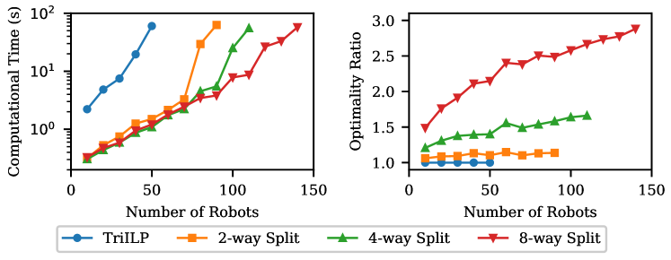
Figure 10: Performance of TriILP with $k$-way split heuristics on a triangular grid with $232$ vertices and varying numbers of robots.

optimally in $60$ seconds. Performance of TriILP is significantly improved with $k$-way split heuristic: with $4$-way split, TriILP can solve problems with $110$ robots in $55$ seconds to $1.65$-optimal. With $8$-way split, we can further push to $140$ robots with reasonable optimality ratio.

Solving (continuous) OLDR requires both DiscretizeOLDR and TriILP. We first attempted a scenario of which the density approaches the theoretical limit by placing the robots just $\frac{8}{3}$ apart from each other in a regular (triangular) pattern for both start and goal configurations (see Fig. 11(a) for an illustration; we omit the labels of the robots, which are different for the start and goal configurations). After running DiscretizeOLDR, we get a discrete arrangement as illustrated in Fig. 11(b). For this particular problem, we can compute a $1.5$-optimal solution in $2.1$ second without using splitting heuristics.

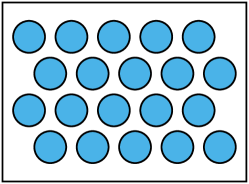
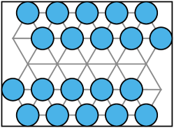
(a)		(b)

Figure 11: Illustration of a compact OLDR instance with $20$ densely packed robots, and the configuration of robots after DiscretizeOLDR.

To test the effectiveness of combining DiscretizeOLDR and TriILP, we constructed many instances similar to Fig. 11 but with different environment sizes, always packing as many robots as possible with separation of exactly $\frac{8}{3}$. The computational performance of this case is compiled in Fig. 12. With the $8$-way split heuristic, our method can solve tightly packed problems of $120$ robots in $21.93$ seconds with a $3.88$ optimality ratio. We note that the (underestimated) optimality ratio in this case actually decreases as the number of robots increases. This is expected because when the number of robots are small, the corresponding environment is also small. The optimality loss due to discretization is more obvious when the environment is smaller.

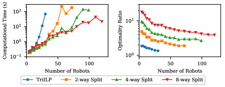
Figure 12: Performance of TriILP (plus DiscretizeOLDR) on dense OLDR instances.

A second evaluation of OLDR carries out a comparison between TriILP (plus DiscretizeOLDR) and HexILP (the main algorithm from [13], which is based on a hexagonal grid discretization). We fix $\mathcal{W}$ with $w=42$ and $h=43.57$; the number of vertices in the triangular grid and hexagonal grid are $312$ and $252$, respectively. For each fixed number of robots $n$, $\mathcal{S}$ and $\mathcal{G}$ are randomly generated within $W$ that are at least $\frac{8}{3}$ apart. Note that this means that collisions may potentially happen for HexILP during the discretization phase, which are ignored (to our disadvantage). The evaluation result is provided in Fig. 13. Since discretization based on triangular grid produces larger models, the running time is generally a bit higher when compared with discretization based on hexagonal grids. However, TriILP can solve problems with many more robots and also produce solutions with much better optimality guarantees.

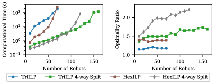
Figure 13: Performance comparison between TriILP and HexILP (with and without $4$-way split heuristic) on randomly generated OLDR instances with a fixed $\mathcal{W}$.

6 Conclusion and Future Work

In this work, we have developed a complete, polynomial-time algorithm for multi-robot routing in a bounded environment under extremely high robot density. The algorithm produces plans that are constant-factor time-optimal. A fast and more practical ILP-based algorithm capable of generating near-optimal solutions is also provided. We mention here that extensions to 3D settings, which may be more applicable to drones and other airborne robot vehicles, can be readily realized under the same framework with only minor adjustments.

Given the theoretical and practical importance of multi-robot (and more generally, multi-agent) routing in crowded settings, in future work, we would like to push robot density to be significantly higher than $50\%$. To achieve this while retaining optimality assurance, we believe the computation-based method developed in this work can be leveraged, perhaps in conjunction with a more sophisticated version of the DiscretizeOLDR algorithm. On the other hand, a triangular grid supports a maximum density of $66\%$; it may be of interest to explore alternatives structures for accommodating denser robot configurations.

References

- [1] J. E. Hopcroft, J. T. Schwartz, and M. Sharir, ``On the complexity of motion planning for multiple independent objects; PSPACE-hardness of the ``warehouseman's problem'','' The International Journal of Robotics Research, vol. 3, no. 4, pp. 76–88, 1984.
- [2] P. Spirakis and C. K. Yap, ``Strong NP-hardness of moving many discs,'' Information Processing Letters, vol. 19, no. 1, pp. 55–59, 1984.
- [3] K. Solovey and D. Halperin, ``On the hardness of unlabeled multi-robot motion planning,'' in Robotics: Science and Systems (RSS), 2015.
- [4] P. R. Wurman, R. D'Andrea, and M. Mountz, ``Coordinating hundreds of cooperative, autonomous vehicles in warehouses,'' AI Magazine, vol. 29, no. 1, pp. 9–19, 2008.
- [5] J. Enright and P. R. Wurman, ``Optimization and coordinated autonomy in mobile fulfillment systems.'' in Automated action planning for autonomous mobile robots, 2011, pp. 33–38.
- [6] M. A. Erdmann and T. Lozano-Pérez, ``On multiple moving objects,'' in Proceedings IEEE International Conference on Robotics & Automation, 1986, pp. 1419–1424.
- [7] S. M. LaValle and S. A. Hutchinson, ``Optimal motion planning for multiple robots having independent goals,'' IEEE Transactions on Robotics & Automation, vol. 14, no. 6, pp. 912–925, Dec. 1998.
- [8] R. Ghrist, J. M. O'Kane, and S. M. LaValle, ``Computing Pareto Optimal Coordinations on Roadmaps,'' International Journal of Robotics Research, vol. 24, no. 11, pp. 997–1010, 2005.
- [9] M. Peasgood, C. Clark, and J. McPhee, ``A complete and scalable strategy for coordinating multiple robots within roadmaps,'' IEEE Transactions on Robotics, vol. 24, no. 2, pp. 283–292, 2008.
- [10] K. Solovey and D. Halperin, ``-color multi-robot motion planning,'' in Proceedings Workshop on Algorithmic Foundations of Robotics, 2012.
- [11] M. Turpin, K. Mohta, N. Michael, and V. Kumar, ``CAPT: Concurrent assignment and planning of trajectories for multiple robots,'' International Journal of Robotics Research, vol. 33, no. 1, pp. 98–112, 2014.
- [12] K. Solovey, J. Yu, O. Zamir, and D. Halperin, ``Motion planning for unlabeled discs with optimality guarantees,'' in Robotics: Science and Systems, 2015.
- [13] J. Yu and D. Rus, ``An effective algorithmic framework for near optimal multi-robot path planning,'' in Robotics Research. Springer, 2018, pp. 495–511.
- [14] S. D. Han, E. J. Rodriguez, and J. Yu, ``Sear: A polynomial-time expected constant-factor optimal algorithmic framework for multi-robot path planning,'' in Proceedings IEEE/RSJ International Conference on Intelligent Robots & Systems, 2018, to appear.
- [15] D. Kornhauser, G. Miller, and P. Spirakis, ``Coordinating pebble motion on graphs, the diameter of permutation groups, and applications,'' in Proceedings IEEE Symposium on Foundations of Computer Science, 1984, pp. 241–250.
- [16] J. Yu, ``Constant factor time optimal multi-robot routing on high-dimensional grid,'' in Robotics: Science and Systems, 2018.
- [17] T. Standley and R. Korf, ``Complete algorithms for cooperative pathfinding problems,'' in Proceedings International Joint Conference on Artificial Intelligence, 2011.
- [18] G. Wagner and H. Choset, ``M*: A complete multirobot path planning algorithm with performance bounds,'' in Proceedings IEEE/RSJ International Conference on Intelligent Robots & Systems, 2011, pp. 3260–3267.
- [19] E. Boyarski, A. Felner, R. Stern, G. Sharon, O. Betzalel, D. Tolpin, and E. Shimony, ``Icbs: The improved conflict-based search algorithm for multi-agent pathfinding,'' in Eighth Annual Symposium on Combinatorial Search, 2015.
- [20] L. Cohen, T. Uras, T. Kumar, H. Xu, N. Ayanian, and S. Koenig, ``Improved bounded-suboptimal multi-agent path finding solvers,'' in International Joint Conference on Artificial Intelligence, 2016.
- [21] J. Yu and S. M. LaValle, ``Optimal multi-robot path planning on graphs: Complete algorithms and effective heuristics,'' IEEE Transactions on Robotics, vol. 32, no. 5, pp. 1163–1177, 2016.
- [22] Gurobi Optimization, Inc., ``Gurobi optimizer reference manual,'' 2018.