Using Swarm Optimization To Enhance Autoencoder’s Images

Abstract

Autoencoders learn data representations through reconstruction. Robust training is the key factor affecting the quality of the learned representations and, consequently, the accuracy of the application that use them. Previous works suggested methods for deciding the optimal autoencoder configuration which allows for robust training. Nevertheless, improving the accuracy of a trained autoencoder has got limited, if no, attention. We propose a new approach that improves the accuracy of a trained autoencoder’s results and answers the following question, Given a trained autoencoder, a test image, and using a real-parameter optimizer, can we generate better quality reconstructed image version than the one generated by the autoencoder?. Our proposed approach combines both the decoder part of a trained Resitricted Boltman Machine-based autoencoder with the Competitive Swarm Optimization algorithm. Experiments show that it is possible to reconstruct images using trained decoder from randomly initialized representations. Results also show that our approach reconstructed better quality images than the autoencoder in most of the test cases. Indicating that, we can use the approach for improving the performance of a pre-trained autoencoder if it does not give satisfactory results.

1 Introduction

Autoencoders are powerful Neural Network (NN) models that learn representations of data with multiple levels of abstraction. Based on the application and the objective measure, the abstract representations are described as “good” if they are useful for addressing tasks of interest  [22]. Examples of these tasks are speech recognition, visual object recognition, image reconstruction and classification.

Learning good discriminative representations using NN-based approaches is very challenging and requires robust training. Factors affecting the training can be related to the network’s configuration, the number of training examples [4] and the lack of proper data preprocessing (engineering) [3]. However, deciding the optimal network configuration is still determined by trail-and-error techniques i.e. by searching through a vast space of possible hypermeter combinations.

Lots of works have been done so far to improve the NNs’, including the autoencoders, accuracy. Most of these works concentrated on the networks’ pre-training (data engineering) and training phases; so new network models were suggested/improved and a few parameter selection methods and principles were suggested [7, 23]. This paper, in contrast, presents a novel approach that improves the accuracy of a pre-trained autoencoder results and answers the following main questions.Without anymore training, is it possible to motivate a pre-trained autoencoder to detect more features?. Given a pre-trained autoencoder, a test image, and using a real-parameter optimizer, can we generate better quality reconstructed version than the autoencoder’s one?

The approach introduced in this paper generates good reconstructed version for given test images using optimized representations. We are applying our approach using a Restricted Boltzmann Machine (RBM)-based autoencoder and the Competitive Swarm Optimization (CSO) algorithm. Only the decoder part of the trained autoencoder is used in conjunction with the (CSO) algorithm to generate optimized representations that produce good reconstructed versions for the target test images.

Our experiments show that it is possible to reconstruct interesting images using the CSO’s particle’s which are used as inputs to the pre-trained decoder. Moreover, our evaluations proved the efficiency of the proposed approach in generating good quality reconstructed versions and allowed the decoder to detect some fine details.

The rest of the paper is organized as follows. In the next section, we cover background about the image representations and briefly present some related works. In the section after that, we describe our proposed new approach. Next, we outline our evaluations. The last two sections conclude our work and present the limitations.

2 Technical Background

2.1 Images Representations and Reconstruction

Images can be generally described using color, shape and texture properties which are extracted using different techniques such as Bag of Words (BoW) [5], Fisher Kernel (FK) [16] and Vector Of Locally Aggregated Descriptors (VLAD) [10]. NN’s representations are other type of representations that can be extracted, after training, by activating a certain layer or a set of layers and concatenating [2, 20] or pooling the results [1]. Such representations are useful for image classification [14],visual object recognition [15], retrieval [17] and reconstruction [11].

Images representation and reconstruction are highly related in the NN world. Dosovitskiyet al,[8], for examples, used a deconvolutional-based approach to reconstruct images from representations learned by a pre-trained deep Convolutional Neural Network (CNN) autoencoders and proved their efficiency in learning deep images representations. Other autoencoder-based techniques such as RBM-based autoencoders [11], discussed in the following subsection, and Stacked Denosing Autoencoders [22] were also introduced to extract robust low dimensional images representations through reconstruction and to reconstruct test images from low dimensional representations.

Generating good image representations that give satisfactory results is still a challenge as it is highly dependent on the robustness of the training process [7]. Neural networks are blackbox predictive tools and designing them require extensive knowledge engineering and careful parameter and configuration decisions [23]. Walczak and Cerpa [23] suggested a set of heuristic principles for designing networks with optimal output performance. Most recently, Ciancio et al, [7] suggested four different heuristic approaches to increase the generalization abilities of a neural network. These methods are based, respectively, on the use of genetic algorithms, Taguchi, tabu search and decision trees. The parameters taken into account are the training algorithm, the number of hidden layers, the number of neurons and the activation function of each hidden layer.

2.2 RBM-based Autoencoder

RBM-based autoencoders were first introduced by Hinton and Ruslan [11] as a non-linear generalization of Principal Component Analysis (PCA). The network consists of an “encoder” part which transforms the high-dimensional input data into a low-dimensional representation (the code), and a “decoder” part which recovers the data (image) from the code.

The autoencoder consists of two-layer RBM network which has stochastic visible and hidden binary units arranged in sublayers using symmetrically weighted connections (weights), Figure 1 depicts an illustration of this.

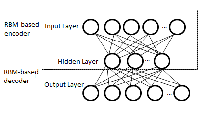
Figure 1: RBM autoencoder

The joint configuration of the visible and hidden units has an energy given by

$$E(v,h)=-\sum_{i\in pixels}b_{i}v_{i}-\sum_{j\in features}b_{j}h_{j}-\sum_{i,j}v_{i}h_{j}w_{ij}$$ (1)

where $v_{i}$ and $h_{j}$ are the binary states of (visible) pixel i and (hidden) feature j respectively; $b_{i}$ and $b_{j}$ are their biases; and $w_{ij}$ is the weight between them.

Starting with random weights, the state of hidden node $h_{j}$ is set to be 1 with a probability defined as :

$$p(h_{j}=1|v)=\sigma(b_{j}+\sum_{i}v_{i}w_{ij})$$ (2)

where $\sigma(x)$ is the logistic function $1/[1+exp(-x)]$.

Once the binary states have been chosen for the hidden nodes, the network sets the visible states by:

$$p(v_{i}=1|h)=\sigma(b_{i}+\sum_{j}h_{j}w_{ij})$$ (3)

where $b_{i}$ is the bias of i.

The states of the hidden nodes are then updated once more so that they represent features of the confabulation. The network tries iteratively to minimize the discrepancy between the input and output data using an optimization algorithm such as gradient descent and propagating the error derivatives through the decoder and then through the encoder networks to fine-tune the weights for optimal reconstruction.

To use the RBM with real-valued images, Ruslan and Hinton  [19] suggested pre-training the network to replace the binary states by stochastic activities. After pretraining, the model unfolds to produce encoder and decoder networks and fine-tunes the weights to replace the stochastic activities by deterministic, real-valued probabilities. Backpropagation is also used through the whole autoencoder to fine-tune the weights for optimal reconstruction.

2.3 Competitive Swarm Optimization (CSO)

CSO [6] is fundamentally inspired by Particle Swarm Optimization (PSO) algorithm [12], which is a conceptually simple optimization algorithm that has attracted considerable research interests so far [21, 13]. PSO defines a swarm of $n$ particles, each of which has a position and velocity flying in an m-dimensional search space. Each particle evaluates the objective function at its current position and iteratively updates its velocity and position according to the particle’s best position, personal best, and the entire swarm global best position found so far. CSO was suggested to overcome the PSO’s poor performance in solving high-dimensional problems and problems with large number of local optima.

In CSO, the swarm’s $n$ particles are randomly allocated into $\frac{n}{2}$ couples and a competition occurs between the two particles in each couple. Only the ones with the better fitness, the winners, are passed to the next generation (iteration), indexed as $t+1$, of the swarm. Each loser particle updates its position and velocity by learning from its winning competitor, and the updated loser is passed to generation $t+1$ after that. Hence, the total number of comparisons occur per generation is $\displaystyle\frac{n}{2}$ and only the velocity and speed for $\displaystyle\frac{n}{2}$ particles are updated per generation. A modified pseudocode of the CSO (with modifications explained in the next section) is given by Algorithm 1.

3 Using The CSO For Enhancing The Autoencoders’ Images

Our main goal is to introduce a novel approach that improves the accuracy of previously trained autoencoder results. The idea of the approach is to use the decoder part of a pre-trained autoencoder and a real-parameter optimizer to reconstruct given test images. To apply the approach, we trained an RBM-based autoencoder and used its decoder with the CSO optimizer. The following subsections presents the methodology and Figure 2 depicts it.

3.1 Training The RBM-based Autoencoder

To train an RBM-based autoencoder according to [11], the network has to be configured by setting the number of input and output layers’ nodes equal to the number of pixels in the training images. Weights and biases are initialized and the network starts learning by feeding the training images through all of its layers to generate output images (reconstructed images) . The discrepancy between the input training image batches and their reconstructed versions are calculated and error derivatives are propagated through the decoder and the encoder parts to fine-tune the weights and biases. After a finite number of iterations, the autoencoder will learn the images’ features, and its encoder part will be ready to generate low dimensional representations for test images that are fed through its input layer. These representations can be used as inputs to the decoder part to reconstruct the input test images or used for other applications.

3.2 Image Reconstruction Using Trained RBM-decoder and CSO

The second step of the approach represents our main contribution in reconstructing an image using a pre-trained decoder with the CSO algorithm. We will refer to our method as decoder+CSO($m$) to indicate the length $m$ of the used representational vector (Algorithm 1).

Contrary to studies that discard the decoder part and use the network’s upper part as a fast image dimensionality reduction method, our novel approach only uses the decoder part of the trained autoencoder and discards the encoder. To generate a reconstructed version $I^{\prime}$ for test image $I$ (Equation 4 ), we feed a swarm $P(t)$ of $n$ randomly initialized low dimensional vectors ($X_{1},..,X_{n}$) through the trained decoder’s layers to get a set of output images $I^{\prime}_{n}$ at its output layer as depicted by Figure 2 step 2. Note that each particle $X_{n}$ is an $m$-dimensional vector and $m$ equals to the number of nodes in the decoder’s first layer i.e. the autoencoder’s bottleneck layer.

$$I^{\prime}=Decoder(X)$$ (4)

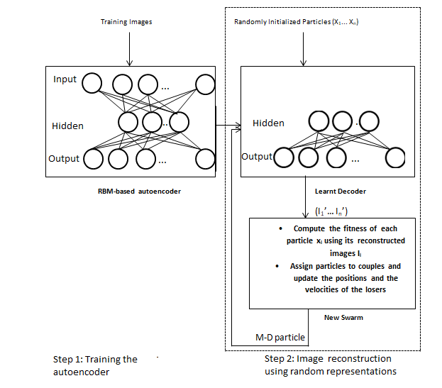
Figure 2: RBM-based autoencoder training and image reconstruction using pre-trained decoder+CSO (m). See Algorithm 1 for better understanding

The Euclidean norm (given by equation 5) between each output image $I^{\prime}_{1..n}$ and the target test image $I$ is computed to identify the fittest individuals.

$$F(X)=||(I-I^{\prime})||_{2}$$ (5)

Where $I^{\prime}$ is the result of decoding representation $X$.

Particles are randomly allocated into $\frac{n}{2}$ couples and the position and velocity of the individuals losing each competition are updated according to their winning partner’s existing velocity and the swarm’s mean velocity as shown in equations 6 & 7) and cited in [6].

$$V_{l,k}(t+1)= R_{1}(k,t)V_{l,k}(t)+R_{2}(k,t)(X_{w,k}(t)-X_{l,k}(t))+$$

$$\varphi R_{3}(k,t)(\bar{X}_{k}(t)-X_{l,k}(t))$$

$$X_{l,k}(t+1)= X_{l,k}(t)+V_{l,k}(t+1).$$ (7)

where $X_{w,k}$, $X_{l,k}$,$V_{w,k}$ and $V_{l,k}$ are the position and velocity of the winner and the loser of generation t respectively, $K\in[1,\frac{n}{2}]$ and $R_{1}(k,t)$, $R_{2}(k,t)$, $R_{3}(k,t)$ $\in$ [0,1]ⁿ are three randomly generated vectors after the k-th round of competition and learning process in generation t, $\bar{X}_{k}(t)$ is the mean position value of the relevant particles and $\varphi$ is a parameter that controls the influence of $\bar{X}_{k}$ (t).

The process of feeding the particles through the decoder part, calculating the fitness function and updating each particle’s positions and velocities are continued for a set of iterations to find the best reconstructed version $I^{\prime}$ for $I$.

1 $t=0$;

2 $count=0$;

3 $I=$target test image ;

4 $Decoder(X)$, the decoder part of a pre-trained autoencoder;

5

6$P(t)$ = $X_{1},X_{2},..,X_{n}$ randomly initialized $m$-dimensional particles;

7 while  terminal condition is not satisfied do

8       feed each element of $P(t)$ through the trained decoder to generate $I^{\prime}_{1},I^{\prime}_{2},..,I^{\prime}_{n}$ using $X_{1},X_{2},..,X_{n}$ according to Equation 4;

9      

10      calculate $F(X)$ between $I$ and $I^{\prime}_{1},I^{\prime}_{2}..I^{\prime}_{n}$ using Equation 5;

11       $U=P(t),O(t+1)=\O$;

12       while $U\neq\O$ do

13             randomly remove two particles $X_{rand1}(t)$, $X_{rand2}(t)$ from U;

14            

15            if $F(X_{rand1}(t))\leq F(X_{rand2}(t))$ then

16                   $X_{w}(t)=X_{rand1}(t),X_{l}(t)=X_{rand2}(t);$

17            else

18                   $X_{w}(t)=X_{rand2}(t),X_{l}(t)=X_{rand1}(t);$

19             end if

20            

21            add $X_{w}(t)$ into $P(t+1)$;

22             update $X_{l}(t)$ using (5) and (6);

23             add the updated $X_{l}(t+1)$ to $P(t+1)$;

24            

25       end while

26      $t=t+1$;

27 end while

Algorithm 1 Image Reconstruction using pre-trained decoder+CSO (m)

Experimental Study

An open-source java-based deep learning library called DeepLearning4j (DL4j) (version 0.7.0) with the MNIST and the OlivettiFaces [18] datasets were used to implement the approach and to perform a set of experiments.

As can be observed by Table 1, the MNIST dataset consists of 60,000 ($28\times 28$) training images for all (0-9) digits. The OlivettiFaces dataset contains ten ($64\times 64$) images for each of forty different people. We constructed a training dataset by rotating (-90 to 270) and subsampling images of 30 people to get 10800 ($22\times 22$) images (i.e. $30\text{ people}\times 10\text{ images per person}\times 36\text{ rotations}$). The 500 OlivettiFaces test images were created in the same way using 10 images of different people. All training and testing images of both datasets were normalized using min-max normalizer to get values in [0-1] range.

Dataset	Dimension	# Training Examples	# Testing Examples	Model Architecture
MNIST	$28\times 28$	60,000	500	784-30-784
MNIST	$28\times 28$	60,000	500	784-250-784
MNIST	$28\times 28$	60,000	500	7841000-500-256-30 -256-500-1000-784
OlivettiFaces	$22\times 22$	10,800 (30 people)	500 (14 people)	484-30-484
OlivettiFaces	$22\times 22$	10,800 (30 people)	500 (14 people)	484-300-484

Table 1: Description of the datasets and network architectures used.

To test the efficiency of the proposed approach, we compared the accuracy of the images reconstructed by the decoder+CSO(m) (optimized) representations with the ones reconstructed by the encoder’s (non-optimized) representations. The trained encoder part of the RBM-based autoencoder was used to generate a low dimensional representation. This representation is fed through the decoder part to generate a reconstructed version of the input test image. Hereafter, we will denote this method by autoencoder($m$) to indicate the length m of the used representational vector.

In all test cases, we set the number of input and output layer’s nodes equals to the training images’ size. All the network’s nodes were initialized using DL4j’s default XAVEIR initialization method where weights are drawn uniformly in the range $[\frac{-2}{\sqrt{In_{l}+Out_{l}}},\frac{2}{\sqrt{In_{l}+Out_{l}}}]$ such that “ $In_{l}$” and “$Out_{l}$” are the number of nodes sending input to and receiving output from the layer ($l$) to be initialized (see [9]). The network was activated by the sigmoid function, and back propagated using the Gradient Descent Optimization algorithm (GDS).

Every trained decoder was used to reconstruct 500 test images using the CSO’s particles. The swarm size was set to 100 randomly initialized [0-1] individuals and the algorithm was run for 100 iterations, which was good enough to evolve interesting results. We also performed experiments using a smaller swarm size (500) and more generations (200), but results were qualitatively very similar to the ones obtained using 100 particles and 100 iterations, so we are only presenting the results of this one.

3.3 Experimental Results and Evaluation

Five experiments, three trained on MNIST dataset and the other two on the OlivettiFaces dataset, were performed using different network models. The aim was to test the accuracy of the proposed approach in reconstructing images from different datasets and using different configurations.

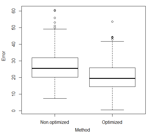
Figure 3: Comparing the performance of autoencoder(30) v.s. decoder+CSO(30) representations in reconstructing MNIST test images.

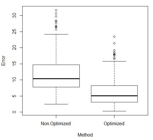
Figure 4: Comparing the performance of autoencoder(250) v.s. decoder+CSO(250) representations in reconstructing MNIST test images.

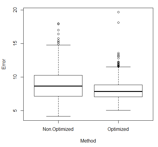
Figure 5: Comparing the performance of autoencoder(30) v.s. decoder+CSO(30) representations in reconstructing OlivittiFaces test images.

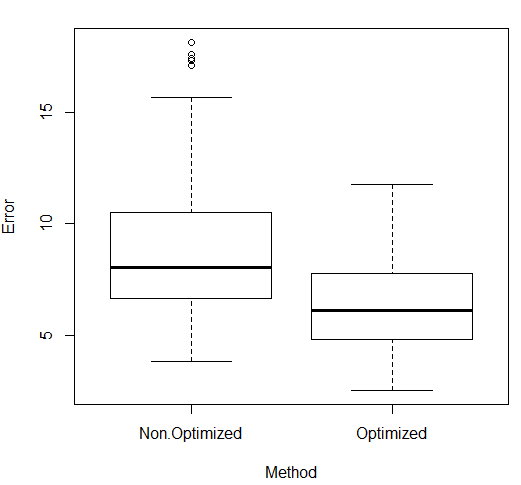
Figure 6: Comparing the performance of autoencoder(300) v.s. decoder+CSO(300) representations in reconstructing OlivittiFaces test images.

Figures 3-7 depict a set of box-and-whisker plots showing the distribution of the error between target original images and reconstructed versions resulting from pre-trained autoencoder(m) and decoder+CSO(m). Comparing the performance of the two methods indicates that the trained decoder+CSO(m) reconstructed better quality images with remarkably less reconstruction error than the trained encoder(m) in most test cases. The decoder+CSO(m) clearly achieved superior results with lowest overall and median reconstruction errors when using three-layered network models for both MNIST datasets (Figures 3-4) and OlivettiFaces dataset (Figure 5-6).

We were also interested in testing our approach using multi layer networks. For fast training, we chose a Multi Layer Percptron (MLP) network configured using nine layers with the following sizes 784-1000-500-256-30-256-500-1000-784. As shown by Figure 7, Optimization added only slight little improvement to the reconstructed images compared to the accuracy of the multi layer autoencoder images.

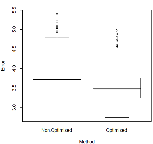
Figure 7: Comparing the performance of multi layer autoencoder(30) v.s. Multi layer decoder+CSO(30) representations in reconstructing MNIST test images.

Qualitative Comparison

Finally we performed qualitative comparisons between all related test cases. As shown by Figures 8-17, the decoder+CSO(m) method reconstructed better quality, less blurry and distorted, MNIST images compared to the autoencoder(m). However, best results obtained, from both methods, when the length of the representational vector was 250.

Experiments on the OlivettiFaces dataset show that the autoencoder(m) method, trained using our parameter settings, was able to efficiently learn the orientation of faces but not their fine details (see Figures 12-15). However, using the optimizer helped in revealing more of the face details.

Results generally indicated that using the CSO real-parameter optimizer enabled the pre-trained network to detect (filter) more of the test images features. Indicating that, the general CSO randomly initialized population was able to activate some of the network’s feature detectors better than the encoder’s representations.

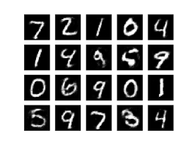
Figure 8: reconstruction of MNIST using decoder+CSO(250) representations.

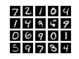
Figure 9: reconstruction of MNIST using autoencoder(250) representations.

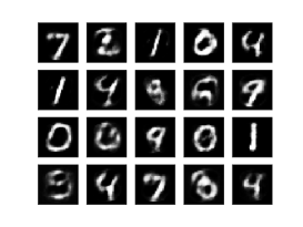
Figure 10: reconstruction of MNIST using decoder+CSO(30) representations.

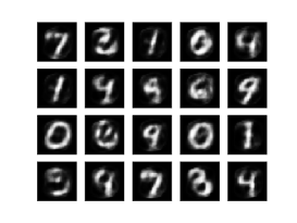
Figure 11: reconstruction of MNIST using autoencoder(30) representations.

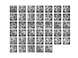
Figure 12: reconstruction of OlivittiFaces using decoder+CSO(30) representations.

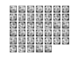
Figure 13: reconstruction of OlivittiFaces using autoencoder(30) representations.

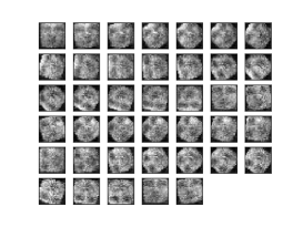
Figure 14: reconstruction of OlivittiFaces using decoder+CSO(300) representations.

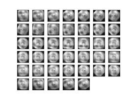
Figure 15: reconstruction of OlivittiFaces using autoencoder(300) representations.

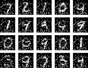
Figure 16: reconstruction of MNIST using Multi layer decoder+CSO(30) representations.

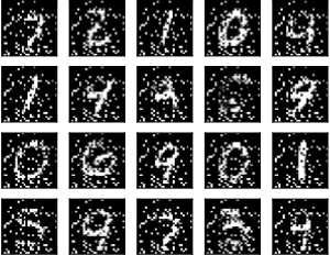
Figure 17: reconstruction of MNIST using Multi layere autoencoder(30) representations.

Conclusion

To conclude, this paper has described a novel approach for improving the performance of previously trained autoencoders. The approach was applied by combining a pre-trained RBM-based decoder with the CSO algorithm and was used to reconstruct a set of test images. Experiments have shown that the suggested approach is able to reconstruct images using randomly initialized representations. The optimization helped in producing sharper images and detecting finer details so it helped in improving the accuracy of pre-trained autoencoder results.

The approach can be applied using other types of autoencoders and/or real-parameter optimizers especially when no satisfactory results obtained from the trained network. In future, we will use the optimized representations in real world biomedical applications.

4 Limitations

Our approach is proposed to improve the accuracy of pre-trained autoencoders results. Reasons affecting the networks performance can be related to the networks’ learning parameters settings and configuration which are determined by trials-and-errors. Using the approach with robustly trained or un-trained networks will add no improvement to the results. The approach is helpful when the network’s neurons are able to detect most of the images features but more accuracy is required. In this case, the optimizer, with its random population, could extract more information from the pre-trained network and increase its ability in detecting fine details and improving the images.

References

- [1] Babenko, A., Lempitsky, V.: Aggregating local deep features for image retrieval. In: Proceedings of the IEEE International Conference on Computer Vision. pp. 1269–1277 (2015)
- [2] Babenko, A., Slesarev, A., Chigorin, A., Lempitsky, V.: Neural codes for image retrieval. In: European Conference on Computer Vision. pp. 584–599. Springer (2014)
- [3] Bengio, Y., Courville, A., Vincent, P.: Representation learning: A review and new perspectives. IEEE transactions on pattern analysis and machine intelligence 35(8), 1798–1828 (2013)
- [4] Bengio, Y., Lamblin, P., Popovici, D., Larochelle, H., et al.: Greedy layer-wise training of deep networks. Advances in Neural Information Processing Systems 19, 153 (2007)
- [5] Bosch, A., Andrew, Z., Muñoz, X.: Scene classification via pLSA. In: European Conference on Computer Vision. pp. 517–530. Springer, Berlin Heidelberg (May 2006)
- [6] Cheng, R., Jin, Y.: A competitive swarm optimizer for large scale optimization. IEEE Transactions on Cybernetics (2), 191–204 (February 2015)
- [7] Ciancio, C., Ambrogio, G., Gagliardi, F., Musmanno, R.: Heuristic techniques to optimize neural network architecture in manufacturing applications. Neural Computing and Applications 27(7), 2001–2015 (2016)
- [8] Dosovitskiy, A., Brox, T.: Inverting visual representations with convolutional networks. In: Proceedings of the IEEE Conference on Computer Vision and Pattern Recognition. pp. 4829–4837 (2016)
- [9] Glorot, X., Bengio, Y.: Understanding the difficulty of training deep feedforward neural networks. Aistats 9, 249–256 (December 2010)
- [10] Hervé, J., Douze, M., Schmid, C., Pérez, P.: Aggregating local descriptors into a compact image representation. In: Computer Vision and Pattern Recognition (CVPR). pp. 3304–3311. IEEE Conference (June 2006)
- [11] Hinton, G., Ruslan, S.R.: Reducing the dimensionality of data with neural networks. Science 313(5786), 504–507 (July 2006)
- [12] Kennedy, J., Eberhart, R.: Particle swarm optimization. IEEE International Conference on Neural Networks (5786), 504–507 (1995)
- [13] Kennedy, J., Mendes, R.: Population structure and particle swarm performance. In: Evolutionary Computation, 2002. CEC’02. Proceedings of the 2002 Congress on 2002. vol. 2, pp. 1931––1938. IEEE (2002)
- [14] Leung, T., Jitendra, M.: Representing and recognizing the visual appearance of materials using three-dimensional textons. International Journal of Computer Vision 43(1) (June 2001)
- [15] Li, L.J., Su, H., Lim, Y., Fei-Fei., L.: Object bank: An object-level image representation for high-level visual recognition. International Journal of Computer Vision 107(1) (March 2014)
- [16] Perronnin, F., Christopher, D.: Fisher kernels on visual vocabularies for image categorization. In: Computer Vision and Pattern Recognition. pp. 1–8. IEEE Conference (June 2007)
- [17] Philbin, J., Ondrej, C., Isard, M., Sivic, J., Zisserman, A.: Object retrieval with large vocabularies and fast spatial matching. In: 2007 IEEE Conference on Computer Vision and Pattern Recognition. IEEE (June 2007)
- [18] Roweis, S.: sam roweis: data.[www page]. URL http://www. cs. nyu. edu/~ roweis/data. html (2012)
- [19] Ruslan, S., Mnih, A., Hinton, G.: Restricted boltzmann machines for collaborative filtering. In: Proceedings of the 24th international conference on machine learning. pp. 791–798. ACM (June 2007)
- [20] Sharif Razavian, A., Azizpour, H., Sullivan, J., Carlsson, S.: CNN features off-the-shelf: an astounding baseline for recognition. In: Proceedings of the IEEE Conference on Computer Vision and Pattern Recognition Workshops. pp. 806–813 (2014)
- [21] Suganthan, P.N.: Particle swarm optimiser with neighbourhood operator. In: CEC 99. Proceedings of IEEE Congress on Evolutionary Computation. pp. 1931––1938. IEEE (1999)
- [22] Vincent, P., Larochelle, H., Lajoie, I., Bengio, Y., Manzago, P.A.: Stacked denoising autoencoders: Learning useful representations in a deep network with a local denoising criterion. Journal of Machine Learning Research 11, 3371–3408 (December 2010)
- [23] Walczak, S., Cerpa, N.: Heuristic principles for the design of artificial neural networks. Information and software technology 41(2), 107–117 (1999)