Prediction of Antiferromagnetism in Barium Chromium Phosphide Confirmed after Synthesis

Abstract

We have carried out density-functional theory (DFT) calculations for the chromium pnictide BaCr₂P₂, which is structurally analogous to BaFe₂As₂, a parent compound for iron-pnictide superconductors. Evolutionary methods combined with DFT predict that the chromium analog has the same crystal structure as the latter. DFT also predicts Néel antiferromagnetic order on the chromium sites. Comparison with a simple electron-hopping model over a square lattice of chromium atoms suggests that it is due to residual nesting of the Fermi surfaces. We have confirmed the DFT predictions directly after the successful synthesis of polycrystalline samples of BaCr₂P₂. X-ray diffraction recovers the predicted crystal structure to high accuracy, while magnetic susceptibility and specific-heat measurements are consistent with a transition to an antiferromagnetically ordered state below $T_{N}\sim 60$ K.

I Introduction

The discovery of iron-pnictide high-temperature superconductors represents one of the most important developments in condensed matter physics over the last ten yearsnew_sc ; paglione_greene_10 . Electric conduction in iron pnictides is due to the iron $3d$ electrons. Elemental iron has six valence electrons in the $3d$ atomic shell, which is one more than half filled. Elemental chromium, on the other hand, has four valence electrons in the $3d$ atomic shell, which is one less than half filled. If Hund’s rule is obeyed, then elemental chromium is the particle-hole conjugate of elemental iron. This observation has motivated a recent search for chromium analogs to iron-pnictide high-temperature superconductors. In particular, the chromium-pnictide compound BaCr₂As₂ has been synthesizedsingh_09 ; filsinger_17 ; richard_17 ; das_17 . It has the same crystal structure asxtal_strctr ThCr₂Si₂, in common with BaFe₂As₂ and with other parent compounds to iron-pnictide superconductors. Also like parent compounds to iron-pnictide superconductors, BaCr₂As₂ is a bad metal that shows antiferromagnetic order on the chromium atoms. Unlike the “stripe” antiferromagnetic order on the iron atoms shown by parent compounds to iron-pnictide superconductors, however, BaCr₂As₂ shows Néel antiferromagnetic order on the chromium atomsfilsinger_17 ; das_17 . All attempts to achieve superconductivity by injecting charge carriers into BaCr₂As₂ through chemical doping have failed so farfilsinger_17 .

Synthesis of the chromium-pnictide sister compound BaCr₂P₂ has been recently reportedbacr2p2 . To our knowledge, however, no report of the measured crystal structure of this new compound has been made in the literature. This has motivated us to perform density-functional theory (DFT) calculations to determine the electronic structure of the new compound. Biologically inspired  optimizationoganov_06 ; lyakhov_13 ; oganov_11 of the crystal structurekresse_93 ; kresse_96 ; kresse_99 results in the expected ThCr₂Si₂-type crystal structure for the groundstatextal_strctr , but with Néel antiferromagnetic order on the chromium atoms. (See Fig. 1.) Analysis of a simple electron hopping model over a square lattice of chromium atoms that contain only the principal $3d_{xz}$ and $3d_{yz}$ orbitals per atom suggests that this Néel order is due to residual nesting of the Fermi surfaces that is hidden by a Lifshitz transition of the latter. We have also succeeded in synthesizing powder samples of the new compound BaCr₂P₂. X-ray diffraction (XRD) on these powders yields lattice constants that agree with our DFT  predictions to within a percent. Last, magnetic susceptibility and specific heat measurements are consistent with a transition from a paramagnetic to an antiferromagnetic state at temperatures below $T_{N}\cong 60$ K.

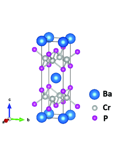
Figure 1: Unit cell of BaCr₂P₂.

II Density-Functional-Theory Calculation

Below, we go into some detail on what evolutionary methods for structure predictions are, followed by what it predicts for the electronic structure of BaCr₂P₂.

II.1 Method

Theoretical prediction of the stable and metastable structures of the compound BaCr₂P₂ was accomplished by using an evolutionary scheme implemented in the code USPEX (Universal Structure Prediction: Evolutionary Xtallography). USPEX was developed by Oganov, Glass, Lyakhov, and Zhuoganov_06 ; lyakhov_13 ; oganov_11 ; it features local optimization, real space representation, and variation operators that mimic natural evolution.

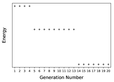
Figure 2: The energy of the best structure predicted by USPEX as a function of the generation number. In the last seven generations, the energy of the best strucure does not change.

The method begins by generating a population of random crystal structures, each with a symmetry prescribed by a randomly chosen space group. For each structure, appropriate lattice vectors and atomic positions are generated in accordance with the selected space group. Density functional theory is then used to optimize the resulting structure and to calculate its free energy (known as the fitness function). Structure optimization is carried out using the VASP code kresse_93 ; kresse_96 ; kresse_99 , which uses a basis set of plane waves to expand the electronic wave function and projector augmented wave (PAW) potentials. Since the generated structures are usually far from equilibrium, the optimization procedure is carried out in four steps, beginning with a coarse optimization, which is followed by successively finer iterations. The set of the optimized structures of the initially generated population constitute the first generation. A new population of crystal structures is then produced, some members of which being randomly generated, while others are obtained as offspring of the best structures (those with lowest energy) of the previous generation. The offspring are derived from parent structures by applying variation operators such as heredity, mutation, or permutation. In each generation, 30% of the structures are generated randomly, 40% by heredity (one structure produced from two parent structures), 10% by soft mutation (atom movements along the softest mode), 10% by lattice mutation (variation of lattice constants), and 10% by permutation (exchanging atoms of different types). The optimized structures in the new population form the second generation, and the best among them serve as precursors for a new generation. The process continues until convergence to the most stable structures is attained. In applying the evolutionary method, an initial population of 200 structures constitutes the first generation; subsequent generations consist of 40 structures each. Convergence to the best structures was achieved after evaluating 960 structures. The structural stability of the best predicted structure is checked by calculating its spectrum of phonon frequencies, using density functional perturbation theory as implemented in Quantum EspressoQE . A grid of $4\times 4\times 4$ $q$-vectors is used to reconstruct the dynamical matrix in real space and subsequently to calculate the phonon frequencies.

As stated above, structure optimization is carried out in four steps that gradually increase in accuracy. In the first, second, third, and fourth steps, the tolerance for the convergence of the self-consistent electronic loop is given by $0.05$ eV, $0.005$ eV, $0.001$ eV, and $0.0001$ eV, respectively. The corresponding values for the ionic relaxation loop are $0.5$ eV, $0.05$ eV, $0.01$ eV, and $0.001$ eV. The Brillouin zone is sampled with a grid spacing given by $2\pi s$ Å^-1, where the grid becomes finer in successive optimization steps, with the parameter $s$ respectively given by $0.12$, $0.10$, $0.08$, and $0.05$ in the first, second, third, and fourth step. The cutoff energies for the plane waves basis set are successively given by $300$ eV, $350$ eV, $420$ eV, and $500$ eV for the four optimization steps. The energy of each optimized structure is finally determined via a static calculation, where the cutoff energy is set to $600$ eV.

For the most stable structure, energy bands and densities of states were calculated using the all-electron, full-potential, linearized, and augmented plane wave methodblaha_01 . Here, space is divided into two regions; one region consists of the interior of non-overlapping spheres (known as muffin-tin spheres) centered at the atomic sites, while the rest of space (the interstitial) forms the other region. The radii of the muffin-tin spheres centered on Ba, Cr, and P were chosen to be $2.50$ a.u., $2.44$ a.u., and $2.00$ a.u., respectively. The basis set used to expand the electronic wave function consists of plane waves in the interstitial, with a maximum wave vector of magnitude $K_{max}$, and where each plane wave is augmented by an atomic-like function in each muffin-tin sphere. The wavenumber $K_{max}$ was chosen so that $K_{max}R_{mt}=8$, where $R_{mt}$ is the radius of the smallest muffin-tin sphere in the unit cell. Charge density was Fourier-expanded up to a maximum wave vector of $14a_{0}^{-1}$, where $a_{0}$ is the Bohr radius. For total energy calculations, a $15\times 15\times 15$ grid of $k$-points was used to integrate functions over the Brillouin zone, and convergence of the self-consistent field calculations was achieved with an energy tolerance of $0.0001$ Ry and a charge tolerance of $0.001e$.

space group (no.)	lattice constants (Å)	angles (degrees)	energy/atom (eV)
I4/mmm (139)	$a=b=3.843$, $c=13.300$	$\alpha=\beta=\gamma=90$	$0.000$
Cm (8)	$a=12.667$, $b=12.367$, $c=4.138$	$\alpha=\beta=90$, $\gamma=160$.9	0.068
P4/mmm (123)	$a=b=3.847$, $c=6.841$	$\alpha=\beta=\gamma=90$	$0.116$

Table 1: The most stable crystal structures of BaCr₂P₂ predicted by evolutionary methods at atmospheric pressure and at zero temperature. The space groups, lattice constants, angles between lattice vectors, and relative energies per atom are listed. For the most stable structure, the fractional coordinate of the phosphorous atom along the $c$-direction is $z=0.35319$ Å. To facilitate comparison, the energy per atom of the most stable structure is set equal to zero.

II.2 Predictions

Figure 2 is a plot of the energy of the best structure, predicted by the evolutionary methods, versus the generation number. In the last seven generations, the energy of the best strucuture is about $1$ meV lower than in previous generations. Table 1 lists the most stable states for BaCr₂P₂ on the basis of evolutionary methods combined with DFT. We should note that in applying the evolutionary methods, we are looking for the best crystal structure of the stoichiometric compound BaCr₂P₂. The groundstate has the ThCr₂Si₂ crystal structurextal_strctr shown in Fig. 1, which is common to the iron and chromium arsenides BaFe₂As₂ and BaCr₂As₂. As shown later, the predicted most stable structure is in excellent agreement with that determined experimentally. To determine the magnetic order in the groundstate, we calculated the energies of structures with different magnetic configuration, using the experimental lattice constants. The results are shown in Table 2. AFM stands for antiferromagnetic, FM for ferromagnetic, and NM for nonmagnetic. In the A-AFM state, the magnetic order is ferromagnetic within the $a$-$b$ plane and antiferromagnetic between the $a$-$b$ planes. In the C-AFM state, the order is ferromagnetic between parallel $a$-$b$ planes, but antiferromagnetic within the planes, while in the G-AFM state, the order is antiferromagnetic both within the $a$-$b$ planes and between the adjacent planes. We conclude that in the groundstate, the magnetic order is three-dimensional (3D) Néel on the chromium atoms. The calculated magnetic moment is approximately $2.93$ Bohr magnetons per chromium atom. The magnetic groundstate according to our DFT calculations is then a spin-$1$ Néel antiferromagnet on the chromium atoms. Figure 3 presents the calculated phonon dispersion curves along high-symmetry directions in the Brillouin zone, along with the phonon density of states. The absence of imaginary frequencies is indicative of the stability of the crystal structure.

magnetic order	energy per formula unit (eV)
G-AFM	0.000
C-AFM	0.016
A-AFM	0.475
FM	0.447
NM	1.620

Table 2: Relative energies per formula unit for various magnetic orders in BaCr₂P₂. Here, NM means nonmagnetic, FM ferromagnetic, and AFM antiferromagnetic. In A-AFM, the order is FM within the $a$-$b$ planes, but AFM between adjacent planes. In C-AFM, the order is AFM within the $a$-$b$ planes, but FM between adjacent planes. In G-AFM, the order is AFM both within the $a$-$b$ planes and between adjacent planes.

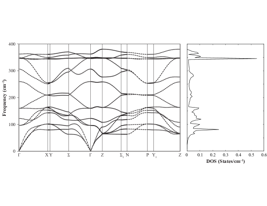
Figure 3: Phonon dispersion curves and density of states predicted by density functional perturbation theory.

Figure 4 shows the energy bands and the density of states predicted by DFT for BaCr₂P₂. The Fermi level lies at zero units of energy. We shall now follow the arguments made by Singh et al. in ref. singh_09 for the case of the sister compound BaCr₂As₂. Notice that the contribution to the density of states that remains after subtracting off the contributions from both the chromium majority-band (Cr1) and the chromium minority-band (Cr2) is sizable at the Fermi level. It is approximately $1/3$ of the total. The remaining contribution to the density of state originates from the phosphorus $3p$ orbitals, which are extended. The latter property accounts for why the contribution due to the phosphorus atoms shown in Fig. 4 is much smaller, where the extended $3p$ states are projected onto the small volume of the phosphorus atoms inside a unit cell. We conclude that like in the case of the sister compoundsingh_09 BaCr₂As₂, a sizable amount of hybridization between the chromium $3d$ states and the phosphorus $3p$ states exists at the Fermi level. This is unlike what occurs in parent compounds to iron-pnictide superconductors such as BaFe₂As₂, in which case the orbital character near the Fermi level is primarily due to the iron $3d$ levels because the pnictogen $3p$ levels are localizedsingh_du_08 ; singh_09 .

Last, Fig. 5 shows the Fermi surfaces predicted for the Néel groundstate by DFT. They are characterized by a 3D Fermi surface pocket centered at the $\Gamma$-point and two tubular Fermi surface sheets along the $c$ axis. Inspection of the band structure shown in Fig. 6 reveals that all three Fermi surface sheets are hole-type. The outer tube shows considerable dispersion along the $c$ axis. These Fermi surfaces resemble those predicted earlier for chromium arsenide by DFTsingh_09 .

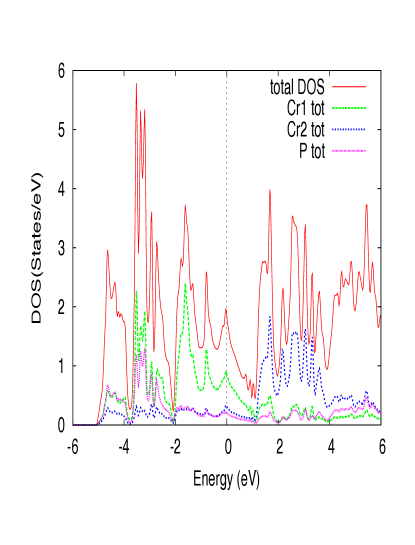
Figure 4: Density of states of BaCr₂P₂ predicted by DFT.

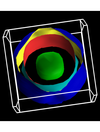
Figure 5: Fermi surfaces of BaCr₂P₂ predicted by DFT.

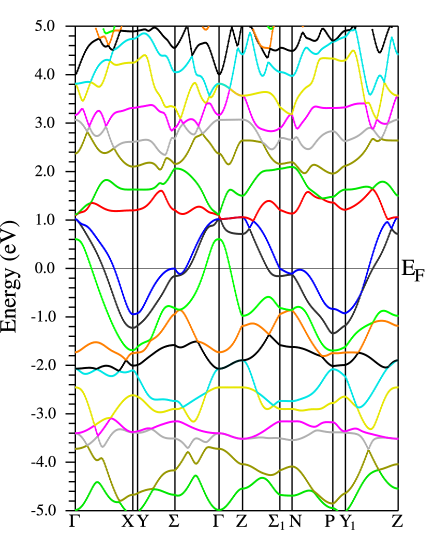
Figure 6: Structure of majority bands in Néel-ordered BaCr₂P₂, as predicted by DFT.

III Experimental Procedures

Below, we report on the successful synthesis of BaCr₂P₂, as well as on X-ray diffraction on the resulting powder samples. Comparison with the previous predictions by DFT of a ThCr₂Si₂-type crystal structure and of a Néel antiferromagnetic groundstate over the chromium atoms is also made.

III.1 Materials Synthesis

The compound BaCr₂P₂ was synthesized using conventional techniques. First, stoichiometric quantities of Ba (Alfa Aesar, Dendritic, 99.9 %), Cr (Alfa Aesar, powder -10+20 mesh, 99.996 %), and P (Alfa Aesar, lump, red 99.999 %) were combined in a stoichiometric quantity inside of a 2 mL volume Al₂O₃ crucible and subsequently sealed under vacuum into a quartz ampoule. Prior to use, the Cr powder was reduced under flowing forming gas (95 % Ar, 5 % H₂) for 12 hours. The ampoule was then placed inside of a box furnace and heated to $500^{\circ}{\rm C}$ over a period of 24 hours and held at this temperature for the same period of time, followed by a ramp-up to $1000^{\circ}{\rm C}$ over 17 hours and a dwell at this last temperature for 24 hours. After this last heat-treatment step, the ampoule was allowed to furnace-cool to room temperature. The mixture was extracted from the crucible, ground and pressed into a pellet in an Ar-filled glovebox, placed in a 2 mL Al₂O₃ crucible, and sealed into a quartz ampoule under 1/3 atm Ar. In this second anneal, the ampoule was taken to $1000^{\circ}{\rm C}$ over a period of 10 hours and held at this temperature for 24 hours, followed by a furnace cool.

The uniformly grey pellet was removed from the ampoule in an Ar-filled glove box and broken into three sections for different materials characterization investigations. We found that the material garnered a greyish-white coating when exposed to air for periods longer than a couple of hours, so we endeavored to minimize exposure as much as possible.

We characterized the structure of the material through X-ray diffraction using a Bruker D8 DaVinci system. In these experiments, we used Co radiation (Co $k_{\alpha}=1.789190\,{\rm\AA})$. We also performed high-temperature diffraction under vacuum using a Perkin Elmer DHS 1100 heater with a graphite dome. FullProf softwareFullProf was used to perform Rietveld refinement on the resultant diffraction patterns. The material was relatively phase-pure ($\sim$ 97 %) and contained only a slight amount of the CrP impurity.

Magnetic and thermal measurements were performed using a Quantum design Model 6000 Physical Property Measurement System (PPMS). The former set of measurements used the VSM option, where we used the profiles of the magnetization versus both the temperature $T$ and the magnetic field $H$ to elucidate the fundamental properties of the polycrystalline sample. In these measurements, we performed a zero-field cool operation before all magnetization versus temperature measurements. The thermal measurements were performed using the heat capacity option. In these measurements, we used the standard pulsed calorimetry option with 2 % temperature rise for the full temperature range and 30 % rise near the phase transition to better characterize the subtle peak we found to be present.

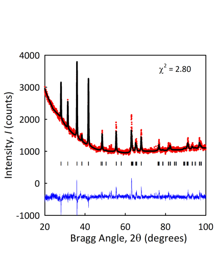
Figure 7: Rietveld fit to the XRD pattern (Co $k_{\alpha}=1.789190{\rm\AA}$) taken for BaCr₂P₂. The red dots represent the collected pattern, the black line is the fit based on the refinement, and the blue line is the difference plot. The hatch marks represent expected peak positions for the refined structure.

III.2 Crystal Structure

We applied full-pattern fitting to our experimental X-ray diffraction data using the FullProf data analysis software packageFullProf . The known structure for BaFe₂P₂ was used as a starting point for our investigationMewis_80 by simply substituting the Cr for the Fe atoms. The resulting fit was of good quality, and it is presented in Fig. 7. With respect to the atomic coordinates within the unit cell, the P position was the only degree of freedom available for fitting. We present the results from the Rietveld analysis in Table 3.

site	$x_{atom}$	$y_{atom}$	$z_{atom}$
barium atom	$0$	$0$	$0$
chromium atom	$1/2$	$0$	$1/4$
phosphorus atom	$0$	$0$	$0.35782(88)$
$R_{p}$	$R_{wp}$	$R_{exp}$	$\chi^{2}$
$3.10$	$4.46$	$2.67$	$2.80$

Table 3: Atomic coordinates and reliability factors from Refined Crystal Structure of BaCr₂P₂ (I4/mmm, No. 139) at $300$ K, where $a=b=3.8472(2)\,{\rm\AA}$ and $c=13.220(12)\,{\rm\AA}$.

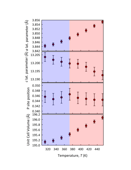
Figure 8: Evolution of structural parameters with temperature.

Like its sister compoundsingh_09 ; filsinger_17 ; das_17 BaCr₂As₂, the crystal structure of BaCr₂P₂ is of the ThCr₂Si₂ type shown in Fig. 1. Further, the crystal structure determined by X-ray diffraction is in excellent agreement with that predicted by DFT, with an error in the lattice constants of less than one percent. It is important to mention that the correct crystal structure predicted by DFT (Table 1) preceded our synthesis of BaCr₂P₂ and the subsequent XRD analysis (Table 3).

We performed high-temperature XRD to determine if any of the anomalies in the magnetization measurements and in the specific heat measurements to be reported below could be ascribed to changes in crystal structure. Figure 8 shows the Rietveld refinements of this experiment. Generally, as temperature is increased, the total thermal expansion is dominated by an increase in the $a$-lattice parameter. At the same time, however, there is a small anomaly in the evolution of the $c$-lattice parameter with temperature that coincides with a small anomaly in the specific heat data reported below. This shift also coincides with a subtle peak in the evolution of the $z$ position of the P atom.

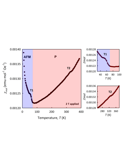
Figure 9: Magnetic susceptibility versus Temperature for BaCr₂P₂.

III.3 Magnetization and Specific Heat

Magnetic Characterization. Magnetization was measured both as a function of temperature for a fixed field and as a function of field for various fixed temperatures spanning the range of the capabilities of our magnetometer (i.e. $1.9-400$ K). We present the zero-field cooled (ZFC) molar susceptibility in Fig. 9. A large paramagnetic signature is present at very low temperatures, likely the result of a small quantity of magnetic impurities being present. Fisher’s analysisfisher_62 of $d(T\chi)/dT$ was used to determine the onset of the two transitions apparent in Fig. 9. We find that the first transition (T1) is at $\sim 60$ K and that the second transition (T2) is at $342.4$ K. Magnetization versus magnetic field ($M(H)$) measurements taken at different temperatures (Fig. 10) are consistent with peak T1 being associated with an antiferromagnetic transition. Further, the temperature dependence shown by the magnetization in Fig. 9 is similar to that shown by related iron-pnictide compoundssaparov_sefat_14 ; sefat_08 ; tegel_08 BaFe₂As₂, SrFe₂As₂, CaFe₂As₂, and SrFeAsF, which also exhibit an antiferromagnetic groundstate. The behavior whereby $\chi$ increases with increasing temperature was qualitatively explained in a simple model by Sales et al. Sales_10 to be ultimately due to the multiband nature of these materials, where both electron and holes are present at the Fermi surface. Interestingly, this model predicts that most semimetals should see an increase in the magnetic susceptibility with increasing temperature.

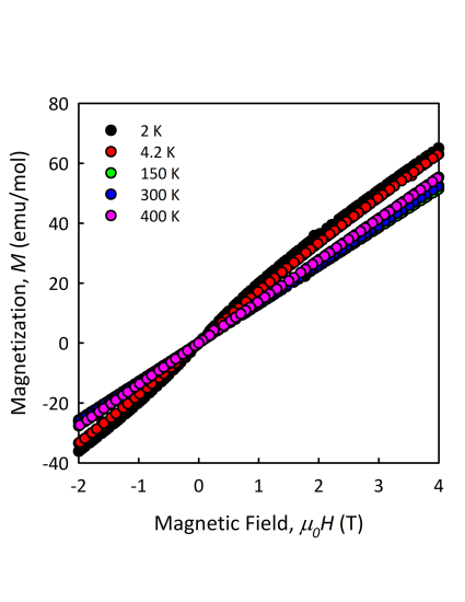
Figure 10: Magnetization curves for BaCr₂P₂.

The peak T2 at higher temperature is consistent with high-temperature XRD data that show a slight inflection in the evolution of the $c/a$ ratio at this temperature. (See Fig. 8.) Future experiments involving single crystals or neutron diffraction measurements will serve to clarify the nature of the magnetism in this material. However, on the basis of our analysis on powder samples, combined with the literature on structurally similar compounds and our DFT calculations above, we posit that the compound BaCr₂P₂ is a G-type antiferromagnet, with a Néel temperature of $\sim 60$ K.

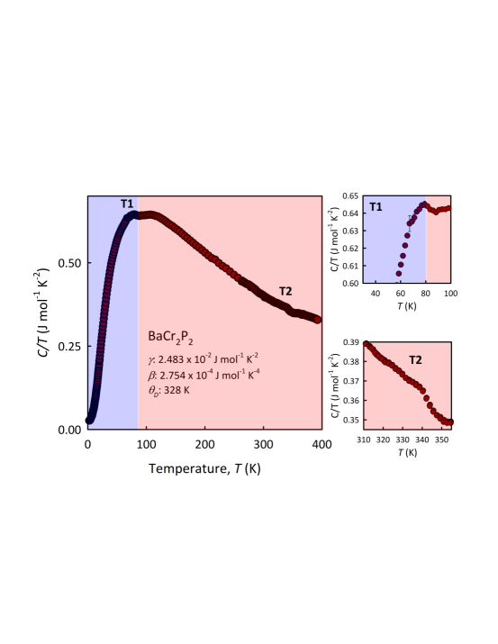
Figure 11: Specific heat versus temperature for the compound BaCr₂P₂. The transitions T1 and T2 are revealed in the two figures on the right-hand panel.

Thermodynamic Characterization. Calorimetric measurements were taken via two different complementary techniques as described in the procedures section. The resulting data are presented in Fig. 11, and they are consistent with the data from magnetization measurements – both transitions T1 and T2 are again present, here at $\sim 75$ K and at $352$ K, in reasonable agreement with the same transitions noted in Fig. 9. Both the high-temperature and low-temperature data are noted in the smaller graphs to the side of the main plot. The data from $2.2$ to $20$ K was fitted to the equation $C/T=\gamma+\beta T^{2}$ to elucidate the Sommerfeld coefficient ($\gamma=24.8$ mJ mol^-1 K^-2) and the Debye temperature ($\theta_{D}=[1944/\beta({\rm mole-atom})]^{1/3}=328$ K) of the compound BaCr₂P₂. For comparison, the Sommerfeld coefficient $\gamma$ for the related G-type antiferromagnet BaCr₂As₂ has been reported with similar valuesfilsinger_17 ; singh_09 : $18.8$-$19.31$ mJ mol^-1 K^-2, with a Debye temperature of $268$ K.

IV Two-orbital hopping model

In section II, we reported that our DFT calculations predict that the groundstate of BaCr₂P₂ is a Néel antiferromagnet over the chromium atoms. The same prediction was made by Singh and coworkers in the case of BaCr₂As₂ singh_09 . Both results raise the following question. What is the physics that underlies the G-type antiferromagnetism in chromium pnictides predicted by DFT? Below, we introduce a tight-binding model that provides some insight into this question.

Our DFT calculation predicts that the electrons at the Fermi level have roughly $2/3$ $d$-orbital character and $1/3$ $p$-orbital character. Importantly, however, the magnetic moment lies exclusively on the chromium site, at which the electron is in the $3d$ orbital. We believe, therefore, that it is sufficient to include only the chromium $3d$ orbitals in order to describe magnetism in chromium pnictides. With this aim in mind, we introduce the following model for an electron that hops over a square lattice of chromium atoms that includes only the principal $3d_{xz}$ and $3d_{yz}$ orbitals:

$$H_{\rm hop}=-\sum_{\langle i,j\rangle}(t_{1}^{\alpha,\beta}c_{i,\alpha,s}^{\dagger}c_{j,\beta,s}+{\rm h.c.})-\sum_{\langle\langle i,j\rangle\rangle}(t_{2}^{\alpha,\beta}c_{i,\alpha,s}^{\dagger}c_{j,\beta,s}+{\rm h.c.}).$$ (1)

We work, specifically, in the isotropic basis of orbitalsjpr_rm_18 $d-=(d_{xz}-id_{yz})/{\sqrt{2}}$ and $d+=(d_{xz}+id_{yz})/{\sqrt{2}}$. Above, $c_{i,\alpha,s}$ and $c_{i,\alpha,s}^{\dagger}$ denote annihilation and creation operators for an electron of spin $s$ in orbital $\alpha$ at site $i$. Repeated indices are summed over. Also above, $\langle i,j\rangle$ and $\langle\langle i,j\rangle\rangle$ represent nearest neighbor (1) and next-nearest neighbor (2) links on the square lattice of chromium atoms.

The reflection symmetries shown by a single layer in a chromium pnictide imply that the above intra-orbital and inter-orbital hopping matrix elements show $s$-wave and $d$-wave symmetry, respectivelyraghu_08 ; Lee_Wen_08 ; jpr_mana_pds_14 . In particular, nearest neighbor hopping matrix elements satisfy

$$t_{1}^{\pm\pm}({\bf{\hat{x}}}) = t_{1}^{\parallel}=t_{1}^{\pm\pm}({\bf{\hat{y}}})$$

$$t_{1}^{\pm\mp}({\bf{\hat{x}}}) = t_{1}^{\perp}=-t_{1}^{\pm\mp}({\bf{\hat{y}}}),$$ (2)

with real $t_{1}^{\parallel}$ and $t_{1}^{\perp}$, while next-nearest neighbor hopping matrix elements satisfy

$$t_{2}^{\pm\pm}({\bf{\hat{x}}}+{\bf{\hat{y}}})=\;t_{2}^{\parallel} = t_{2}^{\pm\pm}({\bf{\hat{y}}}-{\bf{\hat{x}}})$$

$$t_{2}^{\pm\mp}({\bf{\hat{x}}}+{\bf{\hat{y}}})=\pm t_{2}^{\perp} = -t_{2}^{\pm\mp}({\bf{\hat{y}}}-{\bf{\hat{x}}}),$$ (3)

with real $t_{2}^{\parallel}$ and pure-imaginary $t_{2}^{\perp}$.

The above hopping Hamiltonian is easily diagonalized by plane waves of $d_{x(\delta)z}$ and $id_{y(\delta)z}$ orbitals that are rotated with respect to the principal axes by a phase shift $\delta({\bm{k}})$:

$$|{\bm{k}},d_{x(\delta)z}\rangle\rangle = {\cal N}^{-1/2}\sum_{i}e^{i{\bm{k}}\cdot{\bm{r}}_{i}}[e^{i\delta({\bm{k}})}|i,d+\rangle+e^{-i\delta({\bm{k}})}|i,d-\rangle],$$

$$i|{\bm{k}},d_{y(\delta)z}\rangle\rangle = {\cal N}^{-1/2}\sum_{i}e^{i{\bm{k}}\cdot{\bm{r}}_{i}}[e^{i\delta({\bm{k}})}|i,d+\rangle-e^{-i\delta({\bm{k}})}|i,d-\rangle],$$ (4)

where ${\cal N}=2N_{\rm Cr}$ is the number of chromium site-orbitals. Their energy eigenvalues are respectively given by $\varepsilon_{+}({\bm{k}})=\varepsilon_{\parallel}({\bm{k}})+|\varepsilon_{\perp}({\bm{k}})|$ and $\varepsilon_{-}({\bm{k}})=\varepsilon_{\parallel}({\bm{k}})-|\varepsilon_{\perp}({\bm{k}})|$, where

$$\varepsilon_{\parallel}({\bm{k}}) = -2t_{1}^{\parallel}(\cos k_{x}a+\cos k_{y}a)-2t_{2}^{\parallel}(\cos k_{+}a+\cos k_{-}a)$$

$$\varepsilon_{\perp}({\bm{k}}) = -2t_{1}^{\perp}(\cos k_{x}a-\cos k_{y}a)-2t_{2}^{\perp}(\cos k_{+}a-\cos k_{-}a),$$ (5)

are diagonal and off-diagonal matrix elements, with $k_{\pm}=k_{x}\pm k_{y}$. The phase shift $\delta({\bm{k}})$ is set by $\varepsilon_{\perp}({\bm{k}})=|\varepsilon_{\perp}({\bm{k}})|e^{i2\delta({\bm{k}})}$. Specifically,

$$\cos\,2\delta({\bm{k}}) = {-t_{1}^{\perp}(\cos\,k_{x}a-\cos\,k_{y}a)\over{[t_{1}^{\perp 2}(\cos\,k_{x}a-\cos\,k_{y}a)^{2}+|2t_{2}^{\perp}|^{2}(\sin\,k_{x}a)^{2}(\sin\,k_{y}a)^{2}]^{1/2}}},$$

$$\sin\,2\delta({\bm{k}}) = {2(t_{2}^{\perp}/i)(\sin\,k_{x}a)(\sin\,k_{y}a)\over{[t_{1}^{\perp 2}(\cos\,k_{x}a-\cos\,k_{y}a)^{2}+|2t_{2}^{\perp}|^{2}(\sin\,k_{x}a)^{2}(\sin\,k_{y}a)^{2}]^{1/2}}}.$$ (6)

The phase shift is singular at ${\bm{k}}=0$ and $(\pi/a,\pi/a)$, where the matrix element $\varepsilon_{\perp}({\bm{k}})$ vanishes.

If we first turn off next-nearest neighbor intra-orbital hopping, $t_{2}^{\parallel}=0$, notice that the above energy bands then satisfy the perfect nesting condition

$$\varepsilon_{\pm}({\bm{k}}+{\bm{Q}}_{\rm AF})=-\varepsilon_{\mp}({\bm{k}}),$$ (7)

where ${\bm{Q}}_{\rm AF}=(\pi/a,\pi/a)$ is the Néel ordering vector on the square lattice of chromium atoms. As a result, the Fermi level of the bands lies at $\varepsilon_{\rm F}=0$ at half filling. Figure 12a shows such perfectly nested hole-type ($+$) and electron-type ($-$) Fermi surfaces for hopping parameters $t_{1}^{\parallel}=-500$ meV, $t_{1}^{\perp}=-100$ meV, $t_{2}^{\parallel}=0$ and $t_{2}^{\perp}=-100\,i$ meV. Figure 12b, on the other hand, shows residual nesting of the Fermi surfaces at half filling, with hopping parameters $t_{1}^{\parallel}=-500$ meV, $t_{1}^{\perp}=-100$ meV, $t_{2}^{\parallel}=-170$ meV and $t_{2}^{\perp}=-100\,i$ meV. Next-nearest neighbor intra-orbital hopping $t_{2}^{\parallel}$ has been tuned to a Lifshitz transition at which open Fermi surfaces appear. Increasing the strength of $t_{2}^{\parallel}$ past this point results in two hole-type Fermi surfaces at the center of the $1$-chromium Brillouin zone. Such Fermi surface tubes notably resemble the outer tubular Fermi surfaces obtained by DFT that are displayed by Fig. 5.

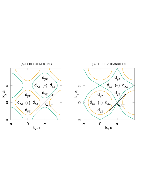
Figure 12: (a) Perfect nesting at wavenumber ${\bm{Q}}_{\rm AF}=(\pi/a,\pi/a)$, with hopping parameters $t_{1}^{\parallel}=-500$ meV, $t_{1}^{\perp}=-100$ meV, $t_{2}^{\parallel}=0$ and $t_{2}^{\perp}=-100\,i$ meV; (b) residual nesting at Lifshitz transition, with $t_{2}^{\parallel}=-170$ meV instead. The “$+$” and “$-$” symbols mark hole-type and electron-type Fermi surfaces, respectively. Both (a) and (b) are at half filling.

The perfectly nested Fermi surfaces shown by Fig. 12a can result in an instability to long-range Néel order. Consider, in particular, the spin magnetization for magnetic order at wave number ${\bm{Q}}$ defined by

$$S_{z}({\bm{Q}})=\sum_{i}\sum_{\alpha}e^{i{\bm{Q}}\cdot{\bm{r}}_{i}}{1\over 2}(n_{i,\alpha,\uparrow}-n_{i,\alpha,\downarrow}).$$ (8)

Here $n_{i,\alpha,s}$ measures the occupation of an electron of spin $s$ in orbital $\alpha$ at site $i$. In momentum space, it takes the form

$$S_{z}({\bm{Q}})={1\over 2}\sum_{s}\sum_{\bm{k}}\sum_{n,n^{\prime}}({\rm sgn}\,s){\cal M}_{n,{\bm{k}};n^{\prime},{\bm{k}}+{\bm{Q}}}\,c_{s}^{\dagger}(n^{\prime},{\bm{k}}+{\bm{Q}})c_{s}(n,{\bm{k}}),$$

(9)

where $c_{s}(n,{\bm{k}})$ and $c_{s}^{\dagger}(n,{\bm{k}})$ are annihilation and creation operators for an electron in eigenstates (4) of the electron hopping Hamiltonian, $H_{\rm hop}$. In particular, $n=1$ and $2$ index the anti-bonding and bonding orbitals $id_{y(\delta)z}$ and $d_{x(\delta)z}$. The above matrix element is computed in ref. jpr_rm_18 . Importantly, at the wave number that corresponds to Néel order, ${\bm{Q}}_{\rm AF}=(\pi/a,\pi/a)$, it is given by

$${\cal M}_{n,{\bm{k}};n^{\prime},{\bm{k}}+{\bm{Q}}_{\rm AF}}=\begin{cases}\pm\sin 2\delta({\bm{k}})&\text{for}\quad n^{\prime}=n,\\ \pm i\cos 2\delta({\bm{k}})&\text{for}\quad n^{\prime}\neq n.\end{cases}$$ (10)

The contribution to the static spin susceptibility from inter-band scattering that corresponds to Néel order is then given by the Lindhard function

$$\chi_{\rm inter}({\bm{Q}}_{\rm AF})=-{1\over{a^{2}N_{\rm Cr}}}\sum_{\bm{k}}{n_{F}[\varepsilon_{-}({\bm{k}}+{\bm{Q}}_{\rm AF})]-n_{F}[\varepsilon_{+}({\bm{k}})]\over{\varepsilon_{-}({\bm{k}}+{\bm{Q}}_{\rm AF})-\varepsilon_{+}({\bm{k}})}}|\cos 2\delta({\bm{k}})|^{2},$$ (11)

where $n_{F}$ is the Fermi-Dirac distribution. Applying the perfect-nesting condition (7) yields the more compact expression

$$\chi_{\rm inter}({\bm{Q}}_{\rm AF})={1\over{a^{2}N_{\rm Cr}}}\sum_{\bm{k}}{{1\over 2}-n_{F}[\varepsilon_{+}({\bm{k}})]\over{\varepsilon_{+}({\bm{k}})}}|\cos 2\delta({\bm{k}})|^{2}.$$ (12)

We conclude that the static susceptibility for Néel order diverges logarithmically as $\chi_{\rm inter}({\bm{Q}}_{\rm AF})={\rm lim}_{\epsilon\rightarrow 0}\,c^{2}D_{+}(0)\,{\rm ln}(W_{\rm bottom}/\epsilon)$, with corresponding density of states weighted by the magnitude square of the matrix element (10):

$$c^{2}D_{+}(\varepsilon)=(2\pi)^{-2}\int_{1\rm Cr\>BZ}d^{2}k\,[\cos 2\delta({\bm{k}})]^{2}\delta[\varepsilon-\varepsilon_{+}({\bm{k}})].$$ (13)

Above, $W_{\rm bottom}=-\varepsilon_{+}(\pi/a,\pi/a)$. The logarithmic divergence of $\chi_{\rm inter}({\bm{Q}}_{\rm AF})$ at perfect nesting guarantees an instability towards long-range Néel order.

Yet can Fermi surfaces that show residual nesting, such as the one displayed by Fig. 12b, also support an instability towards Néel order? To answer this question, we shall compute the static magnetic susceptibility at all wavenumbers. In general, the intra-band and inter-band susceptibilities take the form

$$\chi_{n,n^{\prime}}({\bm{Q}})=-{1\over{a^{2}N_{\rm Cr}}}\sum_{\bm{k}}{n_{F}[\varepsilon_{n^{\prime}}({\bm{k}}+{\bm{Q}})]-n_{F}[\varepsilon_{n}({\bm{k}})]\over{\varepsilon_{n^{\prime}}({\bm{k}}+{\bm{Q}})-\varepsilon_{n}({\bm{k}})}}|{\cal M}_{n,{\bm{k}};n^{\prime},{\bm{k}}+{\bm{Q}}}|^{2}.$$ (14)

The matrix element above has been computed in ref. jpr_rm_18 , and it’s magnitude square is given by

$$|{\cal M}_{n,{\bm{k}};n^{\prime},{\bm{k}^{\prime}}}|^{2}=\begin{cases}\cos^{2}[\delta({\bm{k}})-\delta({\bm{k}^{\prime}})]&\text{for}\quad n^{\prime}=n,\\ \sin^{2}[\delta({\bm{k}})-\delta({\bm{k}^{\prime}})]&\text{for}\quad n^{\prime}\neq n.\end{cases}$$ (15)

Next, the latter can be written in terms of the expressions (6) for ${\rm cos}(2\delta)$ and ${\rm sin}(2\delta)$ by the application of half-angle formulas. The net static spin susceptibility is then $\chi_{0}({\bm{Q}})={1\over 2}\sum_{n=1,2}\sum_{n^{\prime}=1,2}\chi_{n,n^{\prime}}({\bm{Q}})$. Figures 13 and 14 show the static spin susceptibility at perfect nesting and at the Lifshitz transition. Electron hopping parameters are identical to those in Figs. 12a and 12b. Both cases notably show a well-defined peak at ${\bm{Q}}_{\rm AF}$. The logarithmic singularity predicted in the case of perfect nesting is clearly missing in Fig. 13 because the thermodynamic limit has not been achieved.

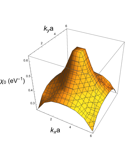
Figure 13: Static spin susceptibility at half filling and at perfect nesting over a $20\times 20$ lattice of chromium atoms. Electron hopping parameters coincide with those in Fig. 12a.

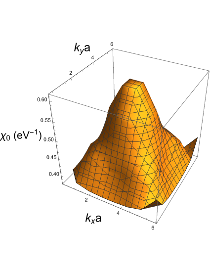
Figure 14: Static spin susceptibility at half filling and at the Lifshitz transition over a $20\times 20$ lattice of chromium atoms. Electron hopping parameters coincide with those in Fig. 12b.

In summary, the present two-orbital hopping model (1) can describe Fermi surface tubes at the center of the $1$-chromium Brillouin zone that resemble qualitatively the outer tubular Fermi surfaces obtained by DFT. (Cf. Figs. 5 and 12b.) Such Fermi surfaces show residual nesting by the Néel wavenumber when they are nearby a Lifshitz transition to open Fermi surfaces. This suggests that similar physics underlies our DFT prediction of Néel antiferromagnetism in chromium pnictides.

V Summary and Conclusions

After performing DFT calculations on the new chromium-pnictide compound BaCr₂P₂, we predict that it has the ThCr₂Si₂ crystal structurextal_strctr , in common with its sister chromium-pnictide compoundsingh_09 ; filsinger_17 BaCr₂As₂. We also successfully synthesized a powder sample of the new material. XRD analysis of the sample yields the predicted crystal structure to within $1$ percent accuracy. Our DFT calculations also predict Néel antiferromagnetism in BaCr₂P₂, with magnetic moments that lie primarily on the chromium atoms. Magnetic susceptibility and specific-heat measurements versus temperature show a kink near $60$ K that we tentatively attribute to the transition temperature for the predicted antiferromagnetic state. Last, by comparison with a simple tight-binding model that contains only the principal $3d_{xz}$ and $3d_{yz}$ orbitals, we suggest that the Néel antiferromagnetic order predicted by DFT is a result of residual nesting of the outer tubular Fermi surfaces that is obscured by a Lifshitz transition. (Cf. Figs. 5 and 12b.)

Unlike iron pnictides, no traces of superconductivity in un-doped or doped chromium pnictides have yet been reported in the literature. Like iron pnictides, however, DFT predicts antiferromagnetic order in chromium-pnictide parent compounds. As mentioned above, it’s quite possible that the previous is due to weak nesting of the tubular Fermi surfaces by the Néel wavenumber. By analogy with the nesting of the hole-type and electron-type Fermi surfaces that exists in parent compounds to iron-pnictide superconductors, a related type of superconductivity may lurk in chromium-pnictide materials that are suitably doped. Indeed, the peak in the static spin susceptibility at the Néel wavevector displayed by Fig. 14 indicates that antiferromagnetic spin fluctuations are present. By analogy with theoretical predictions for the nature of superconductivity in iron-pnictidesmazin_08 ; kuroki_08 , such spin fluctuations can result in $S$-wave Cooper pairing that alternates in sign between the two tubular Fermi surfaces. (See Figs. 5 and 12b.) These theoretical considerations suggest looking for superconductivity in doped BaCr₂P₂ as well.

- (1) Y. Kamihara, T. Watanabe, M. Hirano, and H. Hosono, J. Am. Chem. Soc. 130, 3296 (2008).
- (2) J. Paglione and R.L. Greene, Nature Physics 6, 645 (2010).
- (3) D.J. Singh, A.S. Sefat, M.A. McGuire, B.C. Sales, D. Mandrus, L.H. VanBebber, and V. Keppens, Phys. Rev. B 79, 094429 (2009).
- (4) K.A. Filsinger, W. Schnelle, P. Adler, G.H. Fecher, M. Reehuis, A. Hoser, J.-U. Hoffmann, P. Werner, M. Greenblatt, and C. Felser, Phys. Rev. B 95, 184414 (2017).
- (5) P. Richard, A. van Roekeghem, B.Q. Lv, T. Qian, T.K. Kim, M. Hoesch, J.-P. Hu, A.S. Sefat, S. Biermann, and H. Ding, Phys. Rev. B 95, 184516 (2017).
- (6) P. Das, N.S. Sangeetha, G.R. Lindemann, T.W. Heitmann, A. Kreyssig, A.I. Goldman, R.J. McQueeney, D.C. Johnston, and D. Vaknin, Phys. Rev. B 96, 014411 (2017).
- (7) M. Pfisterer and G. Nagorsen, Z. Naturforsch. B 35, 703 (1980).
- (8) Y. Ichihara, H. Ogino, J. Shimoyama, and K. Kishio, “Development and control of physical properties of new layered compounds with CrPn layers”, Meeting of the American Ceramic Society - Electronic Materials and Applications 2017, January 18-20, 2017, Orlando, Florida.
- (9) A. R. Oganov and C. W. Glass, J. Chem. Phys. 124, 244704 (2006).
- (10) A. O. Lyakhov, A. R. Oganov, H. T. Stokes, and Q. Zhu, Comput. Phys. Commun. 184, 1172 (2013).
- (11) A. R. Oganov, A. O. Lyakhov, and M. Valle, Accounts of Chemical Research 44, 227 (2011).
- (12) G. Kresse and J. Hafner, Phys. Rev. B 47, 558 (1993).
- (13) G. Kresse and J. Furthmüller, Computational Materials Science 6, 15 (1996).
- (14) G. Kresse and D. Joubert, Phys. Rev. B 59, 1758 (1999).
- (15) P. Giannozzi, S. Baroni, N. Bonini, M. Calandra, R. Car, C. Cavazzoni, D. Ceresoli, G. L. Chiarotti, M. Cococcioni, I. Dabo, A. Dal Corso, S. Fabris, G. Fratesi, S. de Gironcoli, R. Gebauer, U. Gerstmann, C. Gougoussis, A. Kokalj, M. Lazzeri, L. Martin-Samos, N. Marzari, F. Mauri, R. Mazzarello, S. Paolini, A. Pasquarello, L. Paulatto, C. Sbraccia, S. Scandolo, G. Sclauzero, A. P. Seitsonen, A. Smogunov, P. Umari, R. M. Wentzcovitch, J. Phys.: Condens. Matter 21, 395502 (2009).
- (16) P. Blaha, K. Schwarz, G. Madsen, D. Kvasnicka, and J. Luitz, “User’s Guide, WIEN2K: An Augmented Plane Wave + Local Orbitals Program for Calculating Crystal Properties”, 2001.
- (17) D.J. Singh and M.-H. Du, Phys. Rev. Lett. 100, 237003 (2008).
- (18) C. Frontera and J. Rodriguez-Carvajal, Physica B: Condensed Matter 350, e731 (2004).
- (19) Albrecht Mewis, Z. Nat. B Chem. Sci. 35, 141 (1980).
- (20) M.E. Fisher, Phil. Mag. 7, 1731 (1962).
- (21) B. Saparov and A.S. Sefat, Dalton Trans. 43, 14971 (2014).
- (22) A.S. Sefat, R.Y. Jin, M.A. McGuire, B.C. Sales, D.J. Singh, D. Mandrus, Phys. Rev. Lett. 101, 117004 (2008).
- (23) M. Tegel, S. Johansson, V. Weiss, I. Schellenberg, W. Hermes, R. Pottgen and D. Johrendt, Euro. Phys. Lett 84, 67007 (2008).
- (24) B.C. Sales, M.A. McGuire, A.S. Sefat, D. Mandrus, Physica C 470, 304 (2010).
- (25) J.P. Rodriguez and R. Melendrez, J. Phys. Commun. 2, 105011 (2018).
- (26) S. Raghu, Xiao-Liang Qi, Chao-Xing Liu, D.J. Scalapino, Shou-Cheng Zhang, Phys. Rev. B 77, 220503(R) (2008).
- (27) P.A. Lee and X.-G. Wen, Phys. Rev. B 78, 144517 (2008).
- (28) J.P. Rodriguez, M.A.N. Araujo, P.D. Sacramento, Eur. Phys. J. B 87, 163 (2014).
- (29) I.I. Mazin, D.J. Singh, M.D. Johannes, and M.H. Du, Phys. Rev. Lett. 101, 057003 (2008).
- (30) K. Kuroki, S. Onari, R. Arita, H. Usui, Y. Tanaka, H. Kontani, and H. Aoki, Phys. Rev. Lett. 101, 087004 (2008).