Glow: Generative Flow
with Invertible 11 Convolutions
Abstract
Flow-based generative models (Dinh et al., , 2014) are conceptually attractive due to tractability of the exact log-likelihood, tractability of exact latent-variable inference, and parallelizability of both training and synthesis. In this paper we propose Glow, a simple type of generative flow using an invertible convolution. Using our method we demonstrate a significant improvement in log-likelihood on standard benchmarks. Perhaps most strikingly, we demonstrate that a generative model optimized towards the plain log-likelihood objective is capable of efficient realistic-looking synthesis and manipulation of large images. The code for our model is available at https://github.com/openai/glow.
1 Introduction
Two major unsolved problems in the field of machine learning are (1) data-efficiency: the ability to learn from few datapoints, like humans; and (2) generalization: robustness to changes of the task or its context. AI systems, for example, often do not work at all when given inputs that are different from their training distribution. A promise of generative models, a major branch of machine learning, is to overcome these limitations by: (1) learning realistic world models, potentially allowing agents to plan in a world model before actual interaction with the world, and (2) learning meaningful features of the input while requiring little or no human supervision or labeling. Since such features can be learned from large unlabeled datasets and are not necessarily task-specific, downstream solutions based on those features could potentially be more robust and more data efficient. In this paper we work towards this ultimate vision, in addition to intermediate applications, by aiming to improve upon the state-of-the-art of generative models.
Generative modeling is generally concerned with the extremely challenging task of modeling all dependencies within very high-dimensional input data, usually specified in the form of a full joint probability distribution. Since such joint models potentially capture all patterns that are present in the data, the applications of accurate generative models are near endless. Immediate applications are as diverse as speech synthesis, text analysis, semi-supervised learning and model-based control; see Section 4 for references.
The discipline of generative modeling has experienced enormous leaps in capabilities in recent years, mostly with likelihood-based methods (Graves, , 2013; Kingma and Welling, , 2013, 2018; Dinh et al., , 2014; van den Oord et al., 2016a, ) and generative adversarial networks (GANs) (Goodfellow et al., , 2014) (see Section 4). Likelihood-based methods can be divided into three categories:
-
1.
Autoregressive models (Hochreiter and Schmidhuber, , 1997; Graves, , 2013; van den Oord et al., 2016a, ; van den Oord et al., 2016b, ; Van Den Oord et al., , 2016). Those have the advantage of simplicity, but have as disadvantage that synthesis has limited parallelizability, since the computational length of synthesis is proportional to the dimensionality of the data; this is especially troublesome for large images or video.
- 2.
- 3.
Flow-based generative models have so far gained little attention in the research community compared to GANs (Goodfellow et al., , 2014) and VAEs (Kingma and Welling, , 2013). Some of the merits of flow-based generative models include:
-
•
Exact latent-variable inference and log-likelihood evaluation. In VAEs, one is able to infer only approximately the value of the latent variables that correspond to a datapoint. GAN’s have no encoder at all to infer the latents. In reversible generative models, this can be done exactly without approximation. Not only does this lead to accurate inference, it also enables optimization of the exact log-likelihood of the data, instead of a lower bound of it.
-
•
Efficient inference and efficient synthesis. Autoregressive models, such as the PixelCNN (van den Oord et al., 2016b, ), are also reversible, however synthesis from such models is difficult to parallelize, and typically inefficient on parallel hardware. Flow-based generative models like Glow (and RealNVP) are efficient to parallelize for both inference and synthesis.
-
•
Useful latent space for downstream tasks. The hidden layers of autoregressive models have unknown marginal distributions, making it much more difficult to perform valid manipulation of data. In GANs, datapoints can usually not be directly represented in a latent space, as they have no encoder and might not have full support over the data distribution. (Grover et al., , 2018). This is not the case for reversible generative models and VAEs, which allow for various applications such as interpolations between datapoints and meaningful modifications of existing datapoints.
-
•
Significant potential for memory savings. Computing gradients in reversible neural networks requires an amount of memory that is constant instead of linear in their depth, as explained in the RevNet paper (Gomez et al., , 2017).
2 Background: Flow-based Generative Models
Let be a high-dimensional random vector with unknown true distribution . We collect an i.i.d. dataset , and choose a model with parameters . In case of discrete data , the log-likelihood objective is then equivalent to minimizing:
| (1) |
In case of continuous data , we minimize the following:
| (2) |
where with , and where is determined by the discretization level of the data and is the dimensionality of . Both objectives (eqs. (1) and (2)) measure the expected compression cost in nats or bits; see (Dinh et al., , 2016). Optimization is done through stochastic gradient descent using minibatches of data (Kingma and Ba, , 2015).
In most flow-based generative models (Dinh et al., , 2014, 2016), the generative process is defined as:
| (3) | ||||
| (4) |
where is the latent variable and has a (typically simple) tractable density, such as a spherical multivariate Gaussian distribution: . The function is invertible, also called bijective, such that given a datapoint , latent-variable inference is done by . For brevity, we will omit subscript from and .
We focus on functions where (and, likewise, ) is composed of a sequence of transformations: , such that the relationship between and can be written as:
| (5) |
Such a sequence of invertible transformations is also called a (normalizing) flow (Rezende and Mohamed, , 2015). Under the change of variables of eq. (4), the probability density function (pdf) of the model given a datapoint can be written as:
| (6) | ||||
| (7) |
where we define and for conciseness. The scalar value is the logarithm of the absolute value of the determinant of the Jacobian matrix , also called the log-determinant. This value is the change in log-density when going from to under transformation . While it may look intimidating, its value can be surprisingly simple to compute for certain choices of transformations, as previously explored in (Deco and Brauer, , 1995; Dinh et al., , 2014; Rezende and Mohamed, , 2015; Kingma et al., , 2016). The basic idea is to choose transformations whose Jacobian is a triangular matrix. For those transformations, the log-determinant is simple:
| (8) |
where takes the sum over all vector elements, takes the element-wise logarithm, and takes the diagonal of the Jacobian matrix.
3 Proposed Generative Flow
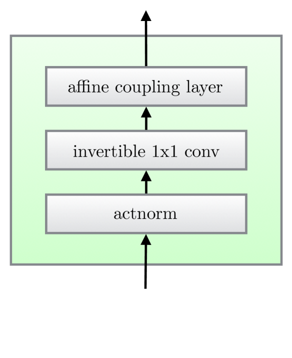
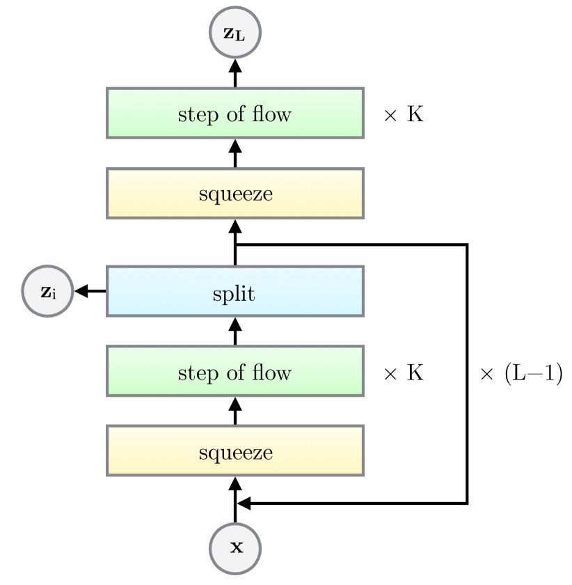
We propose a new flow, building on the NICE and RealNVP flows proposed in (Dinh et al., , 2014, 2016). It consists of a series of steps of flow, combined in a multi-scale architecture; see Figure 2. Each step of flow consists of actnorm (Section 3.1) followed by an invertible convolution (Section 3.2), followed by a coupling layer (Section 3.3).
This flow is combined with a multi-scale architecture; due to space constraints we refer to (Dinh et al., , 2016) for more details. This architecture has a depth of flow , and number of levels (Figure 2).
| Description | Function | Reverse Function | Log-determinant | |||||||||||||||
|---|---|---|---|---|---|---|---|---|---|---|---|---|---|---|---|---|---|---|
|
||||||||||||||||||
|
|
|||||||||||||||||
|
|
|
3.1 Actnorm: scale and bias layer with data dependent initialization
In Dinh et al., (2016), the authors propose the use of batch normalization (Ioffe and Szegedy, , 2015) to alleviate the problems encountered when training deep models. However, since the variance of activations noise added by batch normalization is inversely proportional to minibatch size per GPU or other processing unit (PU), performance is known to degrade for small per-PU minibatch size. For large images, due to memory constraints, we learn with minibatch size 1 per PU. We propose an actnorm layer (for activation normalizaton), that performs an affine transformation of the activations using a scale and bias parameter per channel, similar to batch normalization. These parameters are initialized such that the post-actnorm activations per-channel have zero mean and unit variance given an initial minibatch of data. This is a form of data dependent initialization (Salimans and Kingma, , 2016). After initialization, the scale and bias are treated as regular trainable parameters that are independent of the data.
3.2 Invertible convolution
(Dinh et al., , 2014, 2016) proposed a flow containing the equivalent of a permutation that reverses the ordering of the channels. We propose to replace this fixed permutation with a (learned) invertible convolution, where the weight matrix is initialized as a random rotation matrix. Note that a convolution with equal number of input and output channels is a generalization of a permutation operation.
The log-determinant of an invertible convolution of a tensor with weight matrix is straightforward to compute:
| (9) |
The cost of computing or differentiating is , which is often comparable to the cost computing which is . We initialize the weights as a random rotation matrix, having a log-determinant of 0; after one SGD step these values start to diverge from 0.
LU Decomposition.
This cost of computing can be reduced from to by parameterizing directly in its LU decomposition:
| (10) |
where is a permutation matrix, is a lower triangular matrix with ones on the diagonal, is an upper triangular matrix with zeros on the diagonal, and is a vector. The log-determinant is then simply:
| (11) |
The difference in computational cost will become significant for large , although for the networks in our experiments we did not measure a large difference in wallclock computation time.
In this parameterization, we initialize the parameters by first sampling a random rotation matrix , then computing the corresponding value of (which remains fixed) and the corresponding initial values of and and (which are optimized).
3.3 Affine Coupling Layers
A powerful reversible transformation where the forward function, the reverse function and the log-determinant are computationally efficient, is the affine coupling layer introduced in (Dinh et al., , 2014, 2016). See Table 1. An additive coupling layer is a special case with and a log-determinant of 0.
Zero initialization.
We initialize the last convolution of each with zeros, such that each affine coupling layer initially performs an identity function; we found that this helps training very deep networks.
Split and concatenation.
As in (Dinh et al., , 2014), the function splits the input tensor into two halves along the channel dimension, while the operation performs the corresponding reverse operation: concatenation into a single tensor. In (Dinh et al., , 2016), another type of split was introduced: along the spatial dimensions using a checkerboard pattern. In this work we only perform splits along the channel dimension, simplifying the overall architecture.
Permutation.
Each step of flow above should be preceded by some kind of permutation of the variables that ensures that after sufficient steps of flow, each dimensions can affect every other dimension. The type of permutation specifically done in (Dinh et al., , 2014, 2016) is equivalent to simply reversing the ordering of the channels (features) before performing an additive coupling layer. An alternative is to perform a (fixed) random permutation. Our invertible 1x1 convolution is a generalization of such permutations. In experiments we compare these three choices.
4 Related Work
This work builds upon the ideas and flows proposed in (Dinh et al., , 2014) (NICE) and (Dinh et al., , 2016) (RealNVP); comparisons with this work are made throughout this paper. In (Papamakarios et al., , 2017) (MAF), the authors propose a generative flow based on IAF (Kingma et al., , 2016); however, since synthesis from MAF is non-parallelizable and therefore inefficient, we omit it from comparisons. Synthesis from autoregressive (AR) models (Hochreiter and Schmidhuber, , 1997; Graves, , 2013; van den Oord et al., 2016a, ; van den Oord et al., 2016b, ; Van Den Oord et al., , 2016) is similarly non-parallelizable. Synthesis of high-dimensional data typically takes multiple orders of magnitude longer with AR models; see (Kingma et al., , 2016; Oord et al., , 2017) for evidence. Sampling images with our largest models takes less than one second on current hardware. 111More specifically, generating a image at batch size 1 takes about 130ms on a single 1080 Ti, and about 550ms on a K80
GANs (Goodfellow et al., , 2014) are arguably best known for their ability to synthesize large and realistic images (Karras et al., , 2017), in contrast with likelihood-based methods. Downsides of GANs are their general lack of latent-space encoders, their general lack of full support over the data (Grover et al., , 2018), their difficulty of optimization, and their difficulty of assessing overfitting and generalization.
5 Quantitative Experiments
We begin our experiments by comparing how our new flow compares against RealNVP (Dinh et al., , 2016). We then apply our model on other standard datasets and compare log-likelihoods against previous generative models. See the appendix for optimization details. In our experiments, we let each have three convolutional layers, where the two hidden layers have ReLU activation functions and 512 channels. The first and last convolutions are , while the center convolution is , since both its input and output have a large number of channels, in contrast with the first and last convolution.
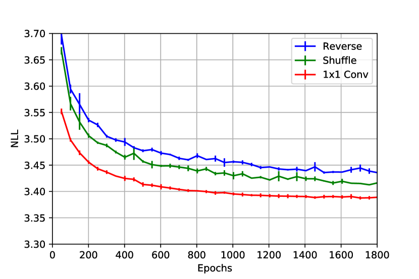
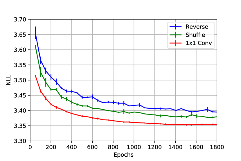
Gains using invertible Convolution.
We choose the architecture described in Section 3, and consider three variations for the permutation of the channel variables - a reversing operation as described in the RealNVP, a fixed random permutation, and our invertible convolution. We compare for models with only additive coupling layers, and models with affine coupling. As described earlier, we initialize all models with a data-dependent initialization which normalizes the activations of each layer. All models were trained with and . The model with convolution has a negligible larger amount of parameters.
We compare the average negative log-likelihood (bits per dimension) on the CIFAR-10 (Krizhevsky, , 2009) dataset, keeping all training conditions constant and averaging across three random seeds. The results are in Figure 3. As we see, for both additive and affine couplings, the invertible convolution achieves a lower negative log likelihood and converges faster. The affine coupling models also converge faster than the additive coupling models. We noted that the increase in wallclock time for the invertible convolution model was only , thus the operation is computationally efficient as well.
Comparison with RealNVP on standard benchmarks.
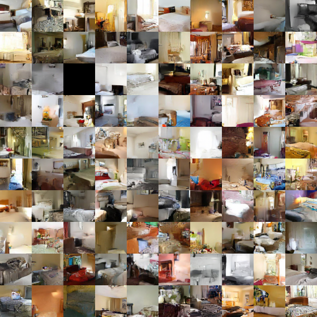
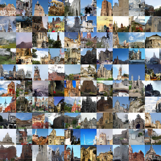
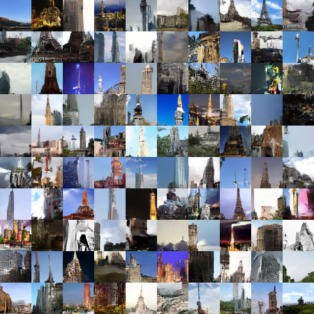
Besides the permutation operation, the RealNVP architecture has other differences such as the spatial coupling layers. In order to verify that our proposed architecture is overall competitive with the RealNVP architecture, we compare our models on various natural images datasets. In particular, we compare on CIFAR-10, ImageNet (Russakovsky et al., , 2015) and LSUN (Yu et al., , 2015) datasets. We follow the same preprocessing as in (Dinh et al., , 2016). For Imagenet, we use the and downsampled version of ImageNet (Oord et al., , 2016), and for LSUN we downsample to and take random crops of . We also include the bits/dimension for our model trained on CelebA HQ used in our qualitative experiments.222Since the original CelebA HQ dataset didn’t have a validation set, we separated it into a training set of 27000 images and a validation set of 3000 images As we see in Table 2, our model achieves a significant improvement on all the datasets.
| Model | CIFAR-10 | ImageNet 32x32 | ImageNet 64x64 | LSUN (bedroom) | LSUN (tower) | LSUN (church outdoor) |
| RealNVP | 2.72 | 2.81 | 3.08 | |||
| Glow |
6 Qualitative Experiments
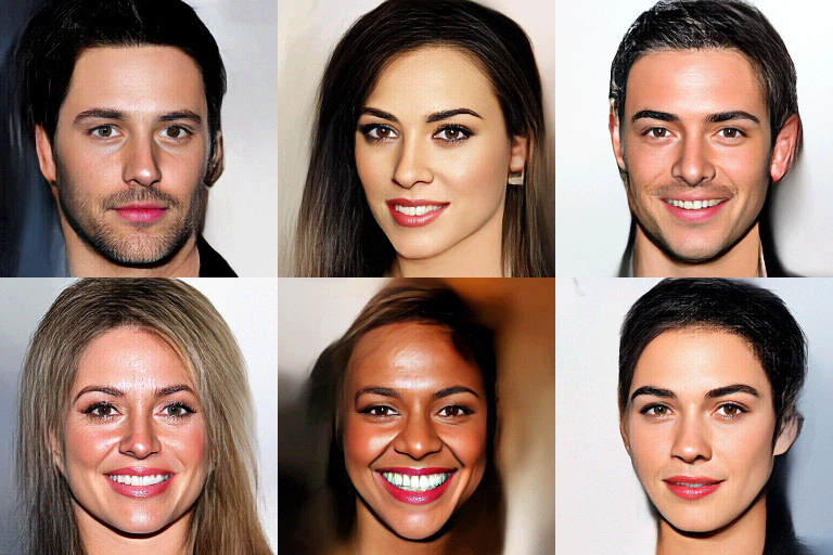
We now study the qualitative aspects of the model on high-resolution datasets. We choose the CelebA-HQ dataset (Karras et al., , 2017), which consists of high resolution images from the CelebA dataset, and train the same architecture as above but now for images at a resolution of , and . To improve visual quality at the cost of slight decrease in color fidelity, we train our models on -bit images. We aim to study if our model can scale to high resolutions, produce realistic samples, and produce a meaningful latent space. Due to device memory constraints, at these resolutions we work with minibatch size 1 per PU, and use gradient checkpointing (Salimans and Bulatov, , 2017). In the future, we could use a constant amount of memory independent of depth by utilizing the reversibility of the model (Gomez et al., , 2017).
Consistent with earlier work on likelihood-based generative models (Parmar et al., , 2018), we found that sampling from a reduced-temperature model often results in higher-quality samples. When sampling with temperature , we sample from the distribution . In case of additive coupling layers, this can be achieved simply by multiplying the standard deviation of by a factor of .
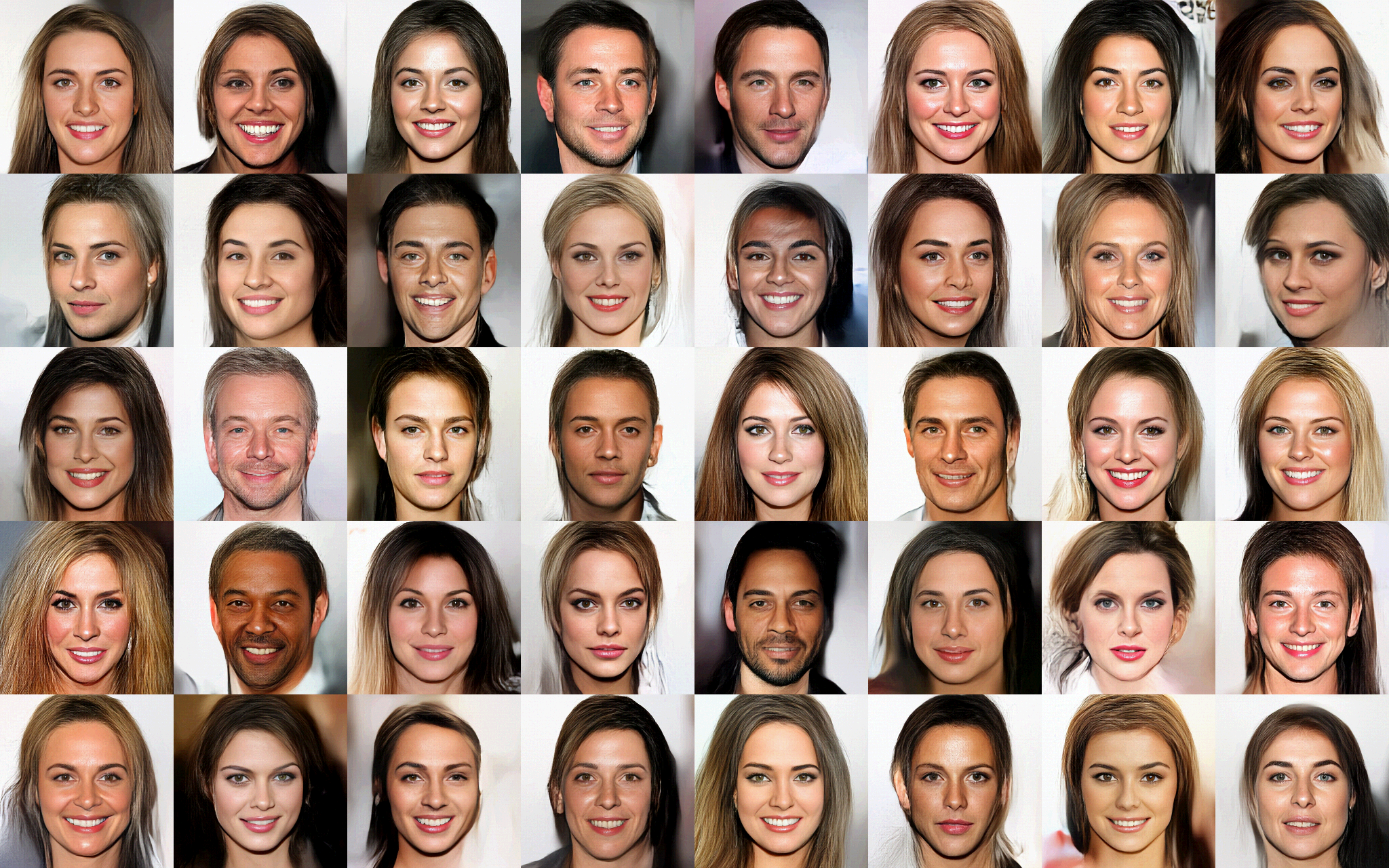
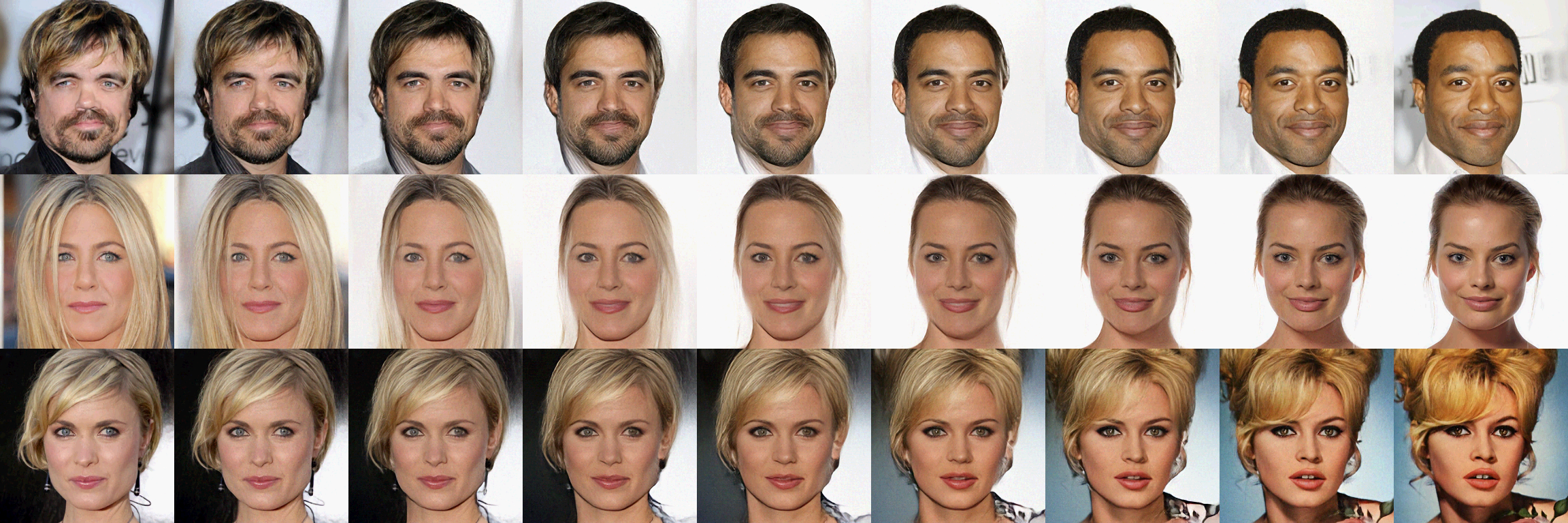
Synthesis and Interpolation.
Figure 4 shows the random samples obtained from our model. The images are extremely high quality for a non-autoregressive likelihood based model. To see how well we can interpolate, we take a pair of real images, encode them with the encoder, and linearly interpolate between the latents to obtain samples. The results in Figure 5 show that the image manifold of the generator distribution is extremely smooth and almost all intermediate samples look like realistic faces.
Semantic Manipulation.
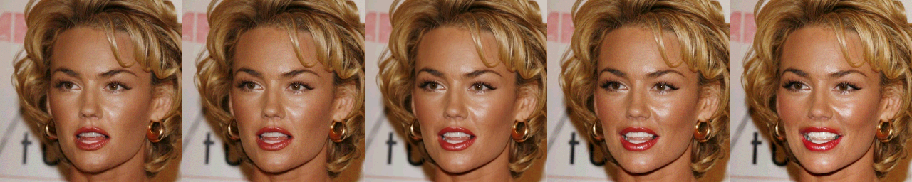
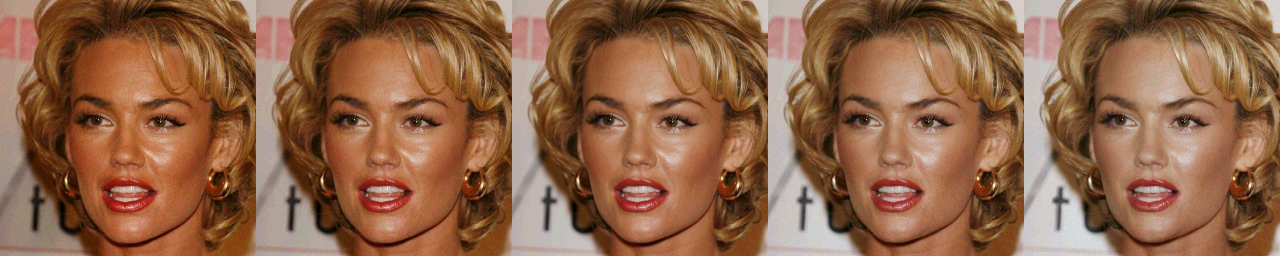
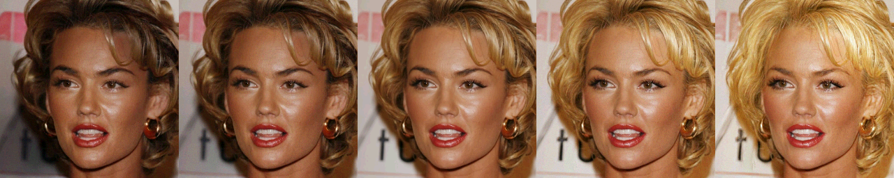
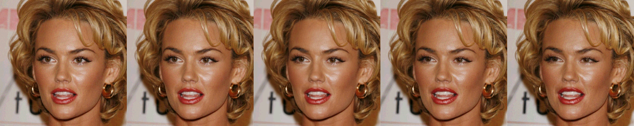
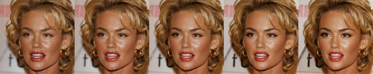
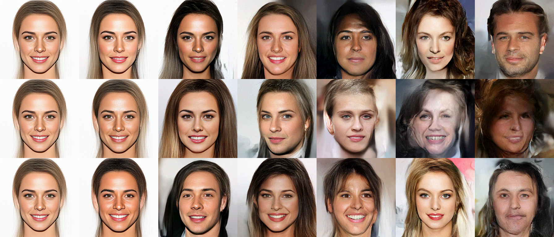
We now consider modifying attributes of an image. To do so, we use the labels in the CelebA dataset. Each image has a binary label corresponding to presence or absence of attributes like smiling, blond hair, young, etc. This gives us binary labels for each attribute. We then calculate the average latent vector for images with the attribute and for images without, and then use the difference as a direction for manipulating. Note that this is a relatively small amount of supervision, and is done after the model is trained (no labels were used while training), making it extremely easy to do for a variety of different target attributes. The results are shown in Figure 6.
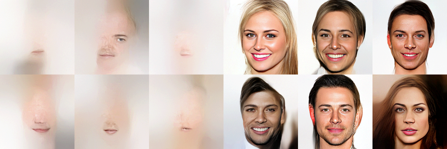
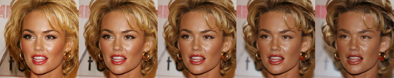
Effect of temperature and model depth.
Figure 8 shows how the sample quality and diversity varies with temperature. The highest temperatures have noisy images, possibly due to overestimating the entropy of the data distribution, and thus we choose a temperature of as a sweet spot for diversity and quality of samples. Figure 9 shows how model depth affects the ability of the model to learn long-range dependencies.
7 Conclusion
We propose a new type of flow, coined Glow, and demonstrate improved quantitative performance in terms of log-likelihood on standard image modeling benchmarks. In addition, we demonstrate that when trained on high-resolution faces, our model is able to synthesize realistic images. Our model is, to the best of our knowledge, the first likelihood-based model in the literature that can efficiently synthesize high-resolution natural images.
References
- Deco and Brauer, (1995) Deco, G. and Brauer, W. (1995). Higher order statistical decorrelation without information loss. Advances in Neural Information Processing Systems, pages 247–254.
- Dinh et al., (2014) Dinh, L., Krueger, D., and Bengio, Y. (2014). Nice: non-linear independent components estimation. arXiv preprint arXiv:1410.8516.
- Dinh et al., (2016) Dinh, L., Sohl-Dickstein, J., and Bengio, S. (2016). Density estimation using Real NVP. arXiv preprint arXiv:1605.08803.
- Gomez et al., (2017) Gomez, A. N., Ren, M., Urtasun, R., and Grosse, R. B. (2017). The reversible residual network: Backpropagation without storing activations. In Advances in Neural Information Processing Systems, pages 2211–2221.
- Goodfellow et al., (2014) Goodfellow, I., Pouget-Abadie, J., Mirza, M., Xu, B., Warde-Farley, D., Ozair, S., Courville, A., and Bengio, Y. (2014). Generative adversarial nets. In Advances in Neural Information Processing Systems, pages 2672–2680.
- Graves, (2013) Graves, A. (2013). Generating sequences with recurrent neural networks. arXiv preprint arXiv:1308.0850.
- Grover et al., (2018) Grover, A., Dhar, M., and Ermon, S. (2018). Flow-gan: Combining maximum likelihood and adversarial learning in generative models. In AAAI Conference on Artificial Intelligence.
- He et al., (2016) He, K., Zhang, X., Ren, S., and Sun, J. (2016). Identity mappings in deep residual networks. arXiv preprint arXiv:1603.05027.
- Hochreiter and Schmidhuber, (1997) Hochreiter, S. and Schmidhuber, J. (1997). Long Short-Term Memory. Neural computation, 9(8):1735–1780.
- Ioffe and Szegedy, (2015) Ioffe, S. and Szegedy, C. (2015). Batch normalization: Accelerating deep network training by reducing internal covariate shift. arXiv preprint arXiv:1502.03167.
- Karras et al., (2017) Karras, T., Aila, T., Laine, S., and Lehtinen, J. (2017). Progressive growing of gans for improved quality, stability, and variation. arXiv preprint arXiv:1710.10196.
- Kingma and Ba, (2015) Kingma, D. and Ba, J. (2015). Adam: A method for stochastic optimization. Proceedings of the International Conference on Learning Representations 2015.
- Kingma et al., (2016) Kingma, D. P., Salimans, T., Jozefowicz, R., Chen, X., Sutskever, I., and Welling, M. (2016). Improved variational inference with inverse autoregressive flow. In Advances in Neural Information Processing Systems, pages 4743–4751.
- Kingma and Welling, (2013) Kingma, D. P. and Welling, M. (2013). Auto-encoding variational Bayes. Proceedings of the 2nd International Conference on Learning Representations.
- Kingma and Welling, (2018) Kingma, D. P. and Welling, M. (2018). Variational autoencoders. Under Review.
- Krizhevsky, (2009) Krizhevsky, A. (2009). Learning multiple layers of features from tiny images.
- Oord et al., (2016) Oord, A. v. d., Kalchbrenner, N., and Kavukcuoglu, K. (2016). Pixel recurrent neural networks. arXiv preprint arXiv:1601.06759.
- Oord et al., (2017) Oord, A. v. d., Li, Y., Babuschkin, I., Simonyan, K., Vinyals, O., Kavukcuoglu, K., Driessche, G. v. d., Lockhart, E., Cobo, L. C., Stimberg, F., et al. (2017). Parallel wavenet: Fast high-fidelity speech synthesis. arXiv preprint arXiv:1711.10433.
- Papamakarios et al., (2017) Papamakarios, G., Murray, I., and Pavlakou, T. (2017). Masked autoregressive flow for density estimation. In Advances in Neural Information Processing Systems, pages 2335–2344.
- Parmar et al., (2018) Parmar, N., Vaswani, A., Uszkoreit, J., Kaiser, Ł., Shazeer, N., and Ku, A. (2018). Image transformer. arXiv preprint arXiv:1802.05751.
- Rezende and Mohamed, (2015) Rezende, D. and Mohamed, S. (2015). Variational inference with normalizing flows. In Proceedings of The 32nd International Conference on Machine Learning, pages 1530–1538.
- Russakovsky et al., (2015) Russakovsky, O., Deng, J., Su, H., Krause, J., Satheesh, S., Ma, S., Huang, Z., Karpathy, A., Khosla, A., Bernstein, M., et al. (2015). Imagenet large scale visual recognition challenge. International Journal of Computer Vision, 115(3):211–252.
- Salimans and Bulatov, (2017) Salimans, T. and Bulatov, Y. (2017). Gradient checkpointing. https://github.com/openai/gradient-checkpointing.
- Salimans and Kingma, (2016) Salimans, T. and Kingma, D. P. (2016). Weight normalization: A simple reparameterization to accelerate training of deep neural networks. arXiv preprint arXiv:1602.07868.
- Van Den Oord et al., (2016) Van Den Oord, A., Dieleman, S., Zen, H., Simonyan, K., Vinyals, O., Graves, A., Kalchbrenner, N., Senior, A., and Kavukcuoglu, K. (2016). Wavenet: A generative model for raw audio. arXiv preprint arXiv:1609.03499.
- (26) van den Oord, A., Kalchbrenner, N., and Kavukcuoglu, K. (2016a). Pixel recurrent neural networks. arXiv preprint arXiv:1601.06759.
- (27) van den Oord, A., Kalchbrenner, N., Vinyals, O., Espeholt, L., Graves, A., and Kavukcuoglu, K. (2016b). Conditional image generation with PixelCNN decoders. arXiv preprint arXiv:1606.05328.
- Yu et al., (2015) Yu, F., Zhang, Y., Song, S., Seff, A., and Xiao, J. (2015). Lsun: Construction of a large-scale image dataset using deep learning with humans in the loop. arXiv preprint arXiv:1506.03365.
Appendix A Additional quantitative results
See Table 3.
| Dataset | Glow |
|---|---|
| CIFAR-10, 3232, 5-bit | 1.67 |
| ImageNet, 3232, 5-bit | 1.99 |
| ImageNet, 6464, 5-bit | 1.76 |
| CelebA HQ, 256256, 5-bit | 1.03 |
Appendix B Simple python implementation of the invertible convolution
Appendix C Optimization details
We use the Adam optimizer (Kingma and Ba, , 2015) with and default and . In out quantitative experiments (Section 5, Table 2) we used the following hyperparameters (Table 4).
| Dataset | Minibatch Size | Levels (L) | Depth per level (K) | Coupling |
|---|---|---|---|---|
| CIFAR-10 | 512 | 3 | 32 | Affine |
| ImageNet, 3232 | 512 | 3 | 48 | Affine |
| ImageNet, 6464 | 128 | 4 | 48 | Affine |
| LSUN, 6464 | 128 | 4 | 48 | Affine |
| Dataset | Minibatch Size | Levels (L) | Depth per level (K) | Coupling |
|---|---|---|---|---|
| LSUN, 6464, 5-bit | 128 | 4 | 48 | Additive |
| LSUN, 9696, 5-bit | 320 | 5 | 64 | Additive |
| LSUN, 128128, 5-bit | 160 | 5 | 64 | Additive |
| CelebA HQ, 256256, 5-bit | 40 | 6 | 32 | Additive |
Appendix D Extra samples from qualitative experiments
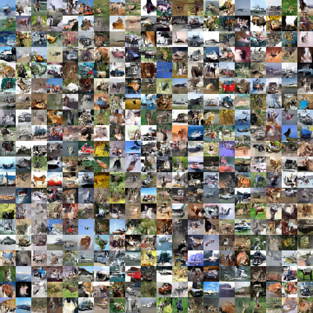
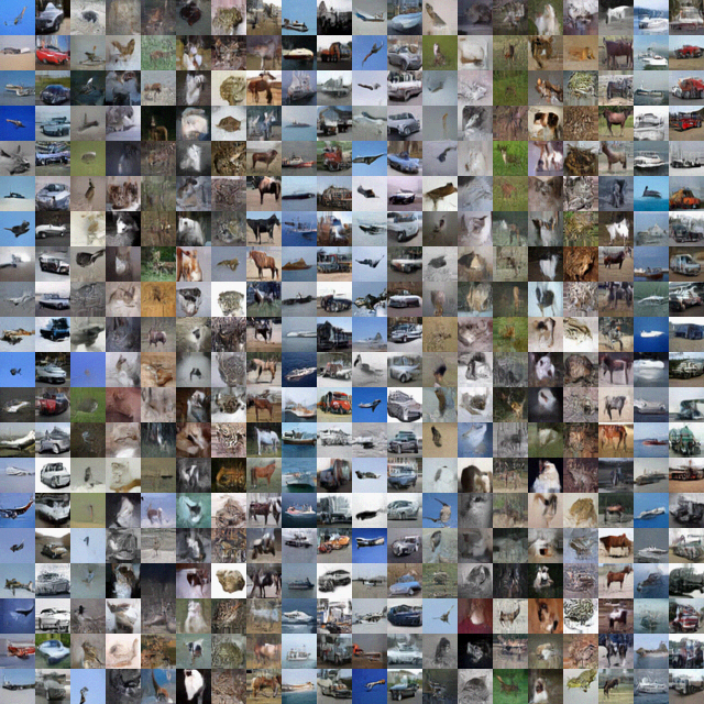
For the class conditional CIFAR-10 and 3232 ImageNet samples, we used the same hyperparameters as the quantitative experiments, but with a class dependent prior at the top-most level. We also added a classification loss to predict the class label from the second last layer of the encoder, with a weight of . The results are in Figure 10.
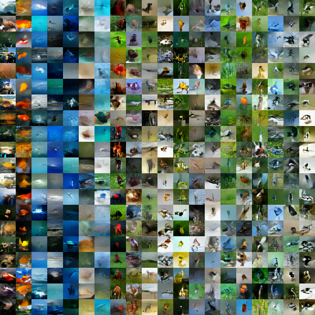
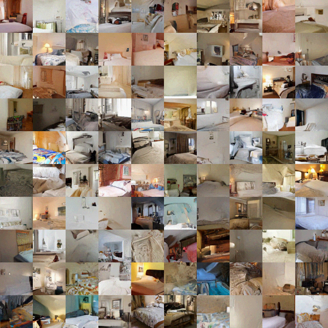
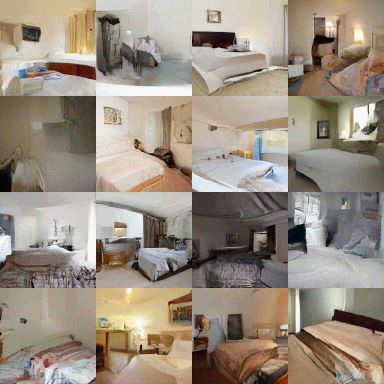
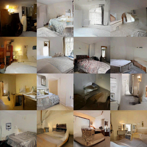
Appendix E Extra samples from the quantitative experiments
For direct comparison with other work, datasets are preprocessed exactly as in Dinh et al., (2016). Results are in Figure 11 and Figure 12.