Quantum Fisher information matrix for unitary processes: closed relation for $SU(2)$

Abstract

Quantum Fisher information plays a central role in the field of quantum metrology. In this paper we study the problem of quantum Fisher information of unitary processes. Associated to each parameter $\theta_{i}$ of unitary process $U(\bm{\theta})$, there exists a unique Hermitian matrix $M_{\theta_{i}}=i(U^{\dagger}\partial_{\theta_{i}}U)$. Except for some simple cases, such as when the parameter under estimation is an overall multiplicative factor in the Hamiltonian, calculation of these matrices is not an easy task to treat even for estimating a single parameter of qubit systems. Using the Bloch vector $\bm{m}_{\theta_{i}}$, corresponding to each matrix $M_{\theta_{i}}$, we find a closed relation for the quantum Fisher information matrix of the $SU(2)$ processes for an arbitrary number of estimation parameters and an arbitrary initial state. We extend our results and present an explicit relation for each vector $\bm{m}_{\theta_{i}}$ for a general Hamiltonian with arbitrary parametrization. We illustrate our results by obtaining the quantum Fisher information matrix of the so-called angle-axis parameters of a general $SU(2)$ process. Using a linear transformation between two different parameter spaces of a unitary process, we provide a way to move from quantum Fisher information of a unitary process in a given parametrization to the one of the other parametrization. Knowing this linear transformation enables one to calculate the quantum Fisher information of a composite unitary process, i.e. a unitary process resulted from successive action of some simple unitary processes. We apply this method for a spin-half system and obtain the quantum Fisher matrix of the coset parameters in terms of the one of the angle-axis parameters.

I Introduction

Estimation theory is an important topic in different areas of physics. Quantum metrology tries to improve estimation precision by using quantum strategy such as entanglement GiovannettiScience2004 ; GiovannettiNatPhot2011 ; HuangAnnual2014 and discord GeorgescuNat2014 ; GiordaPRL2010 ; OllivierPRL2001 . Many applications of quantum metrology have been found, such as gravitational radiation BraginskyPLA2004 ; AdhikariRMP2014 ; McGuirkPRA2002 , quantum frequency standards SantarelliPRL1999 ; BollingerPRA1996 ; HuelgaPRL1997 , quantum imaging TsangPRL2009 ; GiovannettiPRA2009 ; BridaNatPhot2010 , and atomic clocks BuzekPRL1999 ; AndrePRL2004 ; LouchetNJP2010 ; BorregaardPRL2013 ; KesslerPRL2014 . Estimation precision in quantum metrology is described by the Cramer-Rao inequality HolevoBook1982 ; Helstrom1976 ; BraunsteinPRL1994 ; BraunsteinAP1996 ; PetzJPA2002 ; PetzBook2008

$$\delta\theta=\sqrt{\textrm{Var}(\hat{\theta})}\geq\frac{1}{\sqrt{NF_{\theta}}},$$ (1)

where lower bound is related to the inverse of the quantum Fisher information. The estimation precision for separable states is bounded by the standard quantum limit $\Delta\theta\sim\frac{1}{\sqrt{N}}$, whereas for the maximally entangled states, GHZ and NOON states, it is bounded by the Heisenberg limit $\Delta\theta\sim\frac{1}{N}$ (GiovannettiPRL2006, ; LeePRL2006, ; PezzePRL2009, ). In general, there are three stages in quantum metrology: the first is the preparation of the input state, the so-called probe state. In the second stage the input state is encoded with an unknown parameter $\theta$. Finally, the third stage is information extraction, carried out by measuring on the output states. Fisher information is at the heart of metrology and gives us knowledge about the unknown parameters from the probability distribution. It can be obtained directly from its definition $F_{\theta}=\sum_{x}P_{\theta}(x)[\partial_{\theta}\ln P_{\theta}(x)]^{2}$, for discrete outcomes $x$ Fisher1925 , where $P_{\theta}(x)$ is the probability distribution obtained by measuring the encoded probe states. The maximum of $F_{\theta}$ over all possible measurements is the so-called quantum Fisher information (QFI). Quantum Fisher information is related to the Bures BraunsteinPRL1994 ; Bures1969 ; Uhlmann1986 ; HubnerPLA1992 and Hellinger (LuoPRA2004, ) distances which are referred to as two different extensions from classical Fisher information.

Parameter encoding can occur in a noisy SarovarJPA2006 ; MonrasPRL2007 ; WatanabePRL2010 ; LuPRA2010 ; EscherNP2011 ; MaPRA2011 ; ChinPRL2012 ; BerradaPLA2012 ; ZhongPRA2013 ; BerradaPRA2013 ; OzaydinPLA2014 ; AlipourPRL2014 ; BanQIP2015 or noiseless scenario PangPRA2014 ; LiuPA2014 ; LiuCTP2014 ; LiuSR2015 ; JingPRA2015 . In the noiseless encoding, which is the purpose of this work, the parameters are encoded via a unitary operator $U\left(\bm{\theta}\right)$ on an initially $\bm{\theta}$-independent probe state $\rho_{0}$

$$\rho_{\bm{\theta}}=U\left(\bm{\theta}\right)\rho_{0}U^{\dagger}\left(\bm{\theta}\right),$$ (2)

where $\bm{\theta}=\{\theta_{1},\cdots,\theta_{n}\}$ denotes the set of parameters to be encoded. In unitary encoding, the most important ingredients for calculating QFI matrix are the generators of the parameter translations with respect to each parameter $\theta_{i}$ of the unitary process $U(\bm{\theta})$

$$\partial_{\theta_{i}}\rho_{\bm{\theta}}=-i[K_{\theta_{i}},\rho_{\bm{\theta}}].$$ (3)

These generators capture all information of the parametrization process and are defined by BoixoPRL2007

$${K}_{\theta_{i}}=i\frac{\partial U(\bm{\theta})}{\partial{\theta_{i}}}U^{\dagger}(\bm{\theta}),$$ (4)

or equivalently, up to a unitary transformation in the sense of $M_{\theta_{i}}=U^{\dagger}(\bm{\theta}){K}_{\theta_{i}}U(\bm{\theta})$, can be expressed as BoixoPRL2007 ; TaddeiPRL2013

$$M_{\theta_{i}}=iU^{\dagger}(\bm{\theta})\frac{\partial U(\bm{\theta})}{\partial{\theta_{i}}}.$$ (5)

If the unitary process is known, then $K_{\theta_{i}}$ and $M_{\theta_{i}}$ can be directly calculated by their definitions. Also, when the estimation parameter $\theta$ is an overall multiplicative factor of the Hamiltonian, the derivative involved in Eqs. (4) and (5) can be calculated straightforwardly. For estimation of an arbitrary parameter of a $d$-dimensional Hamiltonian, a general solution for $K_{\theta}$ is presented in PangPRA2014

$$K_{\theta} = t\sum_{k=1}^{r}{\mathrm{Tr}}\{\Gamma_{k}^{\dagger}\partial_{\theta}H_{\theta}\}\Gamma_{k}$$

$$- i\sum_{k=r+1}^{d^{2}}\frac{1-{\mathrm{e}}^{-i\lambda_{k}t}}{\lambda_{k}}{\mathrm{Tr}}\{\Gamma_{k}^{\dagger}\partial_{\theta}H_{\theta}\}\Gamma_{k}$$

where $\lambda_{k}$ (with $\lambda_{k}=0$ for $k=1,\cdots,r$ and $\lambda_{k}\neq 0$ for $k=r+1,\cdots,d^{2}$) and $\Gamma_{k}$ are, respectively, eigenvalues and orthonormal eigenvectors of a Hermitian superoperator corresponding to the Hamiltonian $H_{\theta}$, obtained from $[H_{\theta},\Gamma]=\lambda\Gamma$.

Moreover, an expanded form for $\mathcal{H}_{\theta_{i}}=-M_{\theta_{i}}$ is presented in LiuSR2015 which requires calculating an infinite series of

$$\mathcal{H}_{\theta_{i}}=i\sum_{n=0}^{\infty}\mathcal{F}_{n}H_{\bm{\theta}}^{\times n}(\partial_{\theta_{i}}H_{\bm{\theta}}),$$ (7)

where $\mathcal{F}_{n}=(it)^{n+1}/(n+1)!$, $H_{\bm{\theta}}$ is the Hamiltonian of the unitary process $U_{\bm{\theta}}={\mathrm{e}}^{-itH_{\bm{\theta}}}$, and $H^{\times n}(\cdot)=[H,\cdots,[H,\cdot]]$. Utilizing the eigenspectral of $\rho_{0}$

$$\rho_{0}=\sum_{a=0}^{s-1}p_{a}|\varphi_{a}\rangle\langle\varphi_{a}|,$$ (8)

where $\{p_{a}\}_{a=0}^{s-1}$ and $\{|\varphi_{a}\rangle\}_{a=0}^{s-1}$ are the sets of eigenvalues and eigenvectors of $\rho_{0}$, respectively, and $s$ is the dimension of the support of $\rho_{0}$, the matrix elements of QFI for a general unitary transformation $\rho_{\bm{\theta}}=U\left(\bm{\theta}\right)\rho_{0}U^{\dagger}\left(\bm{\theta}\right)$ can be expressed by LiuSR2015 ; LiuCTP2014 ; LiuPA2014

$$F_{\theta_{i}\theta_{j}} = \sum_{a=0}^{s-1}4p_{a}\textrm{cov}_{a}(\mathcal{H}_{\theta_{i}},\mathcal{H}_{\theta_{j}})$$

$$- \sum_{a\neq b}\frac{8p_{a}p_{b}}{p_{a}+p_{b}}\textrm{Re}\left\{\langle\varphi_{a}|\mathcal{H}_{\theta_{i}}|\varphi_{b}\rangle\langle\varphi_{b}|\mathcal{H}_{\theta_{j}}|\varphi_{a}\rangle\right\},$$

where

$$\textrm{cov}_{a}(\mathcal{H}_{\theta_{i}},\mathcal{H}_{\theta_{j}}) = \frac{1}{2}\langle\varphi_{a}|\{\mathcal{H}_{\theta_{i}},\mathcal{H}_{\theta_{j}}\}|\varphi_{a}\rangle$$ (10)

$$- \langle\varphi_{a}|\mathcal{H}_{\theta_{i}}|\varphi_{a}\rangle\langle\varphi_{a}|\mathcal{H}_{\theta_{j}}|\varphi_{a}\rangle$$

is the covariance matrix on the eigenstate $|\varphi_{a}\rangle$ of the initial state LiuSR2015 ; LiuCTP2014 ; LiuPA2014 .

In this paper, we consider the QFI of a unitary process and provide a new representation for QFI of a general $SU(2)$ process. In this representation we associate to each parameter $\theta_{i}$ a real vectors $\bm{m}_{\theta_{i}}\in\mathbb{R}^{3}$. The formulation is independent of the parametrization of the process in a sense that it takes a covariant form for any parametrization of the process. We then provide an explicit relation for the vectors $\bm{m}_{\theta_{i}}$ for a general Hamiltonian with arbitrary parametrization. Furthermore, we present a linear transformation between two different parameter spaces of a unitary process, enabling us to interplay between their corresponding QFI matrices. Using this linear transformation, one can go from either parametrization to another one, in particular, one can obtain the QFI matrix of the coset parameters in terms of the one of the angle-axis parameters.

This paper is organized as follows. In section II, we briefly review the QFI and present a representation for the QFI matrix of a general unitary process in terms of the matrices $\bm{M}_{\theta_{i}}$. We then concern ourselves with the particular case of $SU(2)$ processes and introduce vectors $\bm{m}_{\theta_{i}}$, associated with matrices $\bm{M}_{\theta_{i}}$, and present a closed relation for QFI matrix in terms of these vectors. An analytical closed relation to evaluate these vectors for general Hamiltonian and arbitrary estimation parameters is also provided in this section. Section III is devoted to present a linear transformation between two different parameter spaces of a unitary process. A way to move from QFI matrix of a unitary process in a given parametrization to the one of the other parametrization is provided in this section. The utility of this transformation is examined by providing an example in qubit systems. The paper is concluded in section IV with a brief discussion.

II Quantum Fisher information

From various different versions of QFI, the so-called symmetric logarithmic derivative (SLD) Fisher information is the one which has attracted much attention. For a single parameter $\theta$, the SLD Fisher information is defined by BraunsteinPRL1994 ; BraunsteinAP1996 ; PetzJPA2002 ; PetzBook2008

$$F_{\theta}={\mathrm{Tr}}\left(\rho_{\theta}L_{\theta}^{2}\right),$$ (11)

where $\rho_{\theta}$ is the density matrix depending on $\theta$, and $L_{\theta}$ is the SLD operator determined by the equation

$$\partial_{\theta}\rho_{\theta}=\frac{1}{2} \left\{L_{\theta},\rho_{\theta}\right\},$$ (12)

where $\left\{,\right\}$ denotes anticommutator. For a multiparameter scenario $\bm{\theta}=\{\theta_{1},\cdots,\theta_{n}\}$, the quantum Fisher information matrix is defined by

$$F_{\theta_{i}\theta_{j}}=\frac{1}{2}{\mathrm{Tr}}\left(\rho\left\{L_{\theta_{i}},L_{\theta_{j}}\right\}\right),$$ (13)

where $L_{\theta_{i}}$ is the SLD operator for the parameter $\theta_{i}$, given by

$$\partial_{\theta_{i}}\rho_{\bm{\theta}}=\frac{1}{2}\left\{L_{\theta_{i}},\rho_{\bm{\theta}}\right\},$$ (14)

and $L_{\theta_{j}}$ is defined similarly.

Using the eigenspectral of $\rho_{0}$ given in Eq. (8), one can write the eigenspectral of $\rho_{\bm{\theta}}$ as

$$\rho_{\bm{\theta}}=\sum_{a=0}^{s-1}p_{a}|\tilde{\varphi}_{a}\rangle\langle\tilde{\varphi}_{a}|,$$ (15)

where $|\tilde{\varphi}_{a}\rangle=U\left(\bm{\theta}\right)|\varphi_{a}\rangle$ denotes eigenvectors of $\rho_{\bm{\theta}}$. In this basis Eqs. (3) and (14) read, respectively, as (for $i=1,\cdots,n$)

$$\left(\partial_{\theta_{i}}\rho_{\bm{\theta}}\right)_{\tilde{a}\tilde{b}} = i(p_{a}-p_{b})\left(K_{\theta_{i}}\right)_{\tilde{a}\tilde{b}}$$

$$= \frac{1}{2}(p_{a}+p_{b})\left(L_{\theta_{i}}\right)_{\tilde{a}\tilde{b}},$$

where we have defined $(K_{\theta_{i}})_{\tilde{a}\tilde{b}}=\langle\tilde{\varphi}_{a}|K_{\theta_{i}}|\tilde{\varphi}_{b}\rangle$ and $(L_{\theta_{i}})_{\tilde{a}\tilde{b}}=\langle\tilde{\varphi}_{a}|L_{\theta_{i}}|\tilde{\varphi}_{b}\rangle$. Using this, one can find the matrix elements of the SLD operators in the $\bm{\theta}$-parametrization in terms of the matrix elements of the corresponding matrices $K_{\theta_{i}}$ as

$$(L_{\theta_{i}})_{\tilde{a}\tilde{b}}=2i\frac{\left(p_{a}-p_{b}\right)}{p_{a}+p_{b}}(K_{\theta_{i}})_{\tilde{a}\tilde{b}}.$$ (16)

This can be used in Eq. (13) to find matrix elements of the QFI matrix in the $\bm{\theta}$-representation as

$$F_{\theta_{i}\theta_{j}} = \sum_{a}\sum_{b}2\frac{(p_{a}-p_{b})^{2}}{p_{a}+p_{b}}(K_{\theta_{i}})_{\tilde{a}\tilde{b}}(K_{\theta_{j}})_{\tilde{b}\tilde{a}}$$ (17)

$$= \sum_{a}\sum_{b}2\frac{(p_{a}-p_{b})^{2}}{p_{a}+p_{b}}(M_{\theta_{i}})_{{a}{b}}(M_{\theta_{j}})_{{b}{a}},$$

where $({M}_{\theta_{i}})_{ab}=\langle\varphi_{a}|{M}_{\theta_{i}}|\varphi_{b}\rangle$. Equation (17) provides a relation for the QFI matrix of an arbitrary unitary process $U(\bm{\theta})$, and is equivalent to the one presented by Eq. (I) LiuSR2015 . Accordingly, the QFI matrix can be calculated provided that we could calculate the infinitesimal generators $K_{\theta_{i}}$ (or $M_{\theta_{i}}$) associated to each parameter $\theta_{i}$ ($i=1,\cdots,n$). Instead of using matrix representation of operators, a useful technique is to utilize the Bloch vector representation. This method has been used recently for the SLD operator to derive an explicit expression for the Holevo bound for estimating two-parameter family of qubit states SuzukiIJQI2015 ; SuzukiJMP2016 . In the next section we concern our attention to the $SU(2)$ processes and by using the Bloch vector representation for matrices $M_{\theta_{i}}$, Eq. (5), a closed relation for the QFI matrix of arbitrary parameters of a general Hamiltonian is provided.

II.1 SU(2) processes

For the simplest case of $SU(2)$ processes we will provide a closed relation for Eq. (17) in terms of the Bloch vector representation of the $M$-matrices. To do so, first suppose that the initial state $\rho_{0}$ is diagonal in the computational basis $\{|0\rangle,|1\rangle\}$. In this case Eq. (17) reduces to

$$F_{\theta_{i}\theta_{j}} = 2(p_{0}-p_{1})^{2}\left((M_{\theta_{i}})_{01}(M_{\theta_{j}})_{10}+(M_{\theta_{i}})_{10}(M_{\theta_{j}})_{01}\right)$$ (18)

$$= 2(p_{0}-p_{1})^{2}\left({\mathrm{Tr}}{[M_{\theta_{i}}M_{\theta_{j}}]}-2(M_{\theta_{i}})_{00}(M_{\theta_{j}})_{00}\right),$$

where in the last line we have used the fact that $M$-matrices are traceless. Now, to each Hermitian traceless $2\times 2$ matrix $M_{\theta_{i}}$, one can associate a real vector $\bm{m}_{\theta_{i}}\in\mathbb{R}^{3}$ by $M_{\theta_{i}}=\bm{\sigma}\cdot\bm{m}_{\theta_{i}}$. In this representation we have $(M_{\theta_{i}})_{00}=(\bm{\sigma}\cdot\bm{m}_{\theta_{i}})_{00}=\hat{\bm{z}}\cdot\bm{m}_{\theta_{i}}$ and $M_{\theta_{i}}M_{\theta_{j}}=(\bm{\sigma}\cdot\bm{m}_{\theta_{i}})(\bm{\sigma}\cdot\bm{m}_{\theta_{j}})=(\bm{m}_{\theta_{i}}\cdot\bm{m}_{\theta_{j}}){\mathbb{1}}_{2}+i\bm{\sigma}\cdot(\bm{m}_{\theta_{i}}\times\bm{m}_{\theta_{j}})$. We find

$$F_{\theta_{i}\theta_{j}}=4(p_{0}-p_{1})^{2}\left[\bm{m}_{\theta_{i}}\cdot\bm{m}_{\theta_{j}}-(\hat{\bm{z}}\cdot\bm{m}_{\theta_{i}})(\hat{\bm{z}}\cdot\bm{m}_{\theta_{j}})\right].$$ (19)

In general, however, we are interested in the QFI of the unitary process $U(\bm{\theta})$ starting from an arbitrary initial state $\rho_{0}$ with associated orthonormal eigenbasis $\{|\varphi_{0}\rangle,|\varphi_{1}\rangle\}$. To do this we define $|\varphi_{a}\rangle=\Omega(\theta,\phi)|a\rangle$, for $a=0,1$, with

$$\Omega(\theta,\phi)=\left(\begin{array}[]{cc}\cos{\frac{\theta}{2}}&-{\mathrm{e}}^{-i\phi}\sin{\frac{\theta}{2}}\\ {\mathrm{e}}^{i\phi}\sin{\frac{\theta}{2}}&\cos{\frac{\theta}{2}}\end{array}\right).$$ (20)

One can easily show that $|\varphi_{0}\rangle$ and $|\varphi_{1}\rangle$ are eigenvectors of $\bm{\sigma}\cdot\hat{\bm{n}}$ corresponding to the eigenvalues $+1$ and $-1$, respectively, where $\hat{\bm{n}}=(\sin{\theta}\cos{\phi},\sin{\theta}\sin{\phi},\cos{\theta})^{{\mathrm{t}}}$. Starting from this initial state transforms the $M$-matrices as $M_{\theta_{i}}\rightarrow M_{\theta_{i}}=\Omega^{\dagger}(\theta,\phi)M_{\theta_{i}}\Omega(\theta,\phi)$. Associated to this unitary transformation the $\bm{m}$-vectors rotate as $\bm{m}_{\theta_{i}}\rightarrow O^{\mathrm{t}}\bm{m}_{\theta_{i}}$, where the orthogonal matrix $O$ is defined by $O_{ij}=\frac{1}{2}{\mathrm{Tr}}{[\sigma_{i}\Omega\sigma_{j}\Omega^{\dagger}]}$. Obviously, $\bm{m}_{\theta_{i}}\cdot\bm{m}_{\theta_{j}}$ remains invariant under such transformation and that $\hat{\bm{z}}\cdot O^{\mathrm{t}}\bm{m}_{\theta_{i}}=O\hat{\bm{z}}\cdot\bm{m}_{\theta_{i}}$. Moreover, simple calculation shows that for the unitary transformation (20), $O\hat{\bm{z}}$ is nothing but the unit vector $\hat{\bm{n}}$ defined above. We therefore arrive at the following proposition for the QFI matrix of the unitary process $U(\bm{\theta})\in SU(2)$.

Proposition 1

To each parameter $\theta_{i}$ of the unitary process $U(\bm{\theta})$ one can associate a unique vector $\bm{m}_{\theta_{i}}$ defined by $[\bm{m}_{\theta_{i}}]_{k}=\frac{1}{2}{\mathrm{Tr}}\{\sigma_{k}M_{\theta_{i}}\}$, where $M_{\theta_{i}}$ is given by Eq. (5). Using this, the QFI matrix takes the following form

$$F_{\theta_{i}\theta_{j}} = 4(p_{0}-p_{1})^{2}\left[\bm{m}_{\theta_{i}}^{\mathrm{t}}\Lambda_{\hat{\bm{n}}}\bm{m}_{\theta_{j}}\right]$$

$$= 4(p_{0}-p_{1})^{2}\left[\bm{m}_{\theta_{i}}\cdot\bm{m}_{\theta_{j}}-(\hat{\bm{n}}\cdot\bm{m}_{\theta_{i}})(\hat{\bm{n}}\cdot\bm{m}_{\theta_{j}})\right]$$

where $\Lambda_{\hat{\bm{n}}}={\mathbb{1}}_{3}-\hat{\bm{n}}\hat{\bm{n}}^{\mathrm{t}}$ is a two-dimensional projection operator orthogonal to $\hat{\bm{n}}$.

This simple form shows that the QFI matrix of a unitary process is composed of two independent contributions; first, each parameter $\theta_{i}$ of the unitary process $U(\bm{\theta})$ is contributed in the Fisher information via the vector $\bm{m}_{\theta_{i}}\in\mathbb{R}^{3}$, and second, the role of the initial state $\rho_{0}$ is played by the Bloch vector $\hat{\bm{n}}$ and the eigenvalues $p_{0},p_{1}$. However, looking at Eq. (1) shows that although $\bm{m}_{\theta_{i}}$ are vectors in $\mathbb{R}^{3}$, their role in the QFI matrix is played effectively in a two dimensional subspace perpendicular to $\hat{\bm{n}}$. To see this note that $\bm{m}_{\theta_{i}}^{\mathrm{t}}\Lambda_{\hat{\bm{n}}}\bm{m}_{\theta_{j}}=(\Lambda_{\hat{\bm{n}}}\bm{m}_{\theta_{i}})^{\mathrm{t}}(\Lambda_{\hat{\bm{n}}}\bm{m}_{\theta_{j}})$ and $\Lambda_{\hat{\bm{n}}}\bm{m}_{\theta_{i}}\in\mathrm{Range}\{\Lambda_{\hat{\bm{n}}}\}$. Accordingly, initial states with different Bloch vectors result in different subspaces, hence different QFI matrix, in general. It turns out that the QFI matrix is invariant under orthogonal transformation on the vectors $\bm{m}_{\theta_{i}}$, i.e. $\bm{m}_{\theta_{i}}\longrightarrow R\bm{m}_{\theta_{i}}$, provided that the Bloch vector of the initial state is changed as $\hat{\bm{n}}\longrightarrow R^{\mathrm{t}}\hat{\bm{n}}$. In view of this, the maximum of QFI matrix over all initial states, if exists, is invariant under orthogonal transformation performed on $\bm{m}_{\theta_{i}}$. For instance, for a single parameter $\theta$, Eq. (1) reduces to $F_{\theta}=4(p_{0}-p_{1})^{2}\left[|\bm{m}_{\theta}|^{2}-(\hat{\bm{n}}\cdot\bm{m}_{\theta})^{2}\right]$, implies that the QFI attains its maximum value $F_{\theta}^{\max}=4|\bm{m}_{\theta}|^{2}$, gained by any initial pure state $|\bm{\sigma}\cdot\hat{\bm{n}}\rangle$ with $\hat{\bm{n}}$ lying in the plane perpendicular to $\bm{m}_{\theta}$.

Another consequence of Eq. (1) is that the lack of independency of the vectors $\bm{m}_{\theta_{i}}$ leads to vanishing determinant of the QFI matrix, meaning that the variances of the set of parameters cannot be estimated simultaneously through the Cramer-Rao bound. To make an interpretation of this, suppose $\bm{m}_{\theta_{k}}=\sum_{l\neq k}c_{l}\bm{m}_{\theta_{l}}$ for some nonzero real numbers $c_{l}$. In this case we find $M_{\theta_{k}}=\sum_{l\neq k}c_{l}M_{\theta_{l}}$, results in $\frac{\partial U(\bm{\theta})}{\partial{\theta_{k}}}=\sum_{l\neq k}c_{l}\frac{\partial U(\bm{\theta})}{\partial{\theta_{l}}}$ from Eq. (5). Defining $U(\bm{\theta})={\mathrm{e}}^{-iHt}$ for Hamiltonian $H$ and invoking Eq. (24), we find $\frac{\partial H}{\partial{\theta_{k}}}=\sum_{l\neq k}c_{l}\frac{\partial H}{\partial{\theta_{l}}}$. The converse is also true meaning that any relation between derivatives of the Hamiltonian leads to the same relation between the corresponding $\bm{m}$-vectors, as such, for any initial probe state $\rho_{0}$ the QFI matrix becomes singular. What is noteworthy here is that the lack of independency of $\bm{m}$-vectors is not necessary to get singular QFI matrix, as Eq. (1) could lead to a singular QFI matrix even for linearly independent $\bm{m}$-vectors. To see this consider, for example, two arbitrary parameters $\theta_{1}$ and $\theta_{2}$ associated with two linearly independent vectors $\bm{m}_{\theta_{1}}$ and $\bm{m}_{\theta_{2}}$. One can see that for any Bloch vector of the initial state lying in the plane of $\bm{m}_{\theta_{1}}$ and $\bm{m}_{\theta_{2}}$, i.e. for any $\hat{\bm{n}}=a_{1}\bm{m}_{\theta_{1}}+a_{2}\bm{m}_{\theta_{2}}$ with arbitrary real numbers $a_{1}$ and $a_{2}$ such that $a_{1}^{2}|\bm{m}_{\theta_{1}}|^{2}+a_{2}^{2}|\bm{m}_{\theta_{2}}|^{2}+2a_{1}a_{2}\bm{m}_{\theta_{1}}\cdot\bm{m}_{\theta_{2}}=1$, the QFI matrix obtained from Eq. (1) has a vanishing determinant.

Moreover, for the eigendecomposition of $\rho_{\bm{\theta}}$, given by Eq. (15), one can see that $F(\rho_{\bm{\theta}})=(p_{0}-p_{1})^{2}F(\tilde{\varphi}_{a})$ for $a=0,1$, as such $F(\rho_{\bm{\theta}})/\sum_{a=0}^{1}p_{a}F(\tilde{\varphi}_{a})=(p_{0}-p_{1})^{2}\leq 1$, implies convexity of the QFI in this case.

Having Eq. (1) as a relation for QFI matrix in terms of the vectors $\bm{m}_{\theta_{i}}$, it is now the time to present a relation to calculate the required vectors $\bm{m}_{\theta_{i}}$ for a general Hamiltonian. The following proposition provides an explicit representation for vectors $\bm{m}_{\theta_{i}}$ of a general qubit Hamiltonian.

Proposition 2

For a unitary process generated by the Hamiltonian JingPRA2015

$$H=\bm{\alpha}\cdot\bm{\sigma},$$ (22)

the associated $\bm{m}$-vectors are given by the following relation

$$\bm{m}_{\theta_{i}}=\frac{\partial{|\bm{\alpha}|}}{\partial{\theta_{i}}}t\;\hat{\bm{\alpha}} + \sin{(|\bm{\alpha}|t)}\cos{(|\bm{\alpha}|t)}\frac{\partial{\hat{\bm{\alpha}}}}{\partial{\theta_{i}}}$$

$$- \sin^{2}{(|\bm{\alpha}|t)}\left(\hat{\bm{\alpha}}\times\frac{\partial{\hat{\bm{\alpha}}}}{\partial{\theta_{i}}}\right),$$

where we have defined the unit vector $\hat{\bm{\alpha}}=\bm{\alpha}/|\bm{\alpha}|$.

Before we proceed further to provide a proof for the above equation, we have to stress here that a similar relation, however with different derivation, is provided in Ref. JingPRA2015 .

• Using the equation WilcoxJMP1967

  $$\frac{\partial}{\partial\theta_{i}}{\mathrm{e}}^{-iHt}=\int_{0}^{1}{\mathrm{e}}^{-isHt}\left(-it\frac{\partial}{\partial\theta_{i}}H\right){\mathrm{e}}^{-i(1-s)Ht}{\mathrm{d}}s,$$ (24)

  in the definition of $[\bm{m}_{\theta_{i}}]_{k}$, we get

  $$[\bm{m}_{\theta_{i}}]_{k} = \frac{i}{2}{\mathrm{Tr}}\left\{\sigma_{k}U^{\dagger}(\bm{\theta})\frac{\partial U(\bm{\theta})}{\partial{\theta_{i}}}\right\}$$ (25)

  $$= \frac{t}{2}\int_{0}^{1}{\mathrm{d}}s\;{\mathrm{Tr}}\left\{V(s)\sigma_{k}V^{\dagger}(s)\frac{\partial H}{\partial{\theta_{i}}}\right\}$$

  $$= t\sum_{l=1}^{3}\frac{\partial\alpha_{l}}{\partial{\theta_{i}}}\int_{0}^{1}{\mathrm{d}}s\;O_{lk}(s),$$

  where we have defined $V(s)={\mathrm{e}}^{-i(1-s)Ht}$, and $O_{lk}(s)=\frac{1}{2}{\mathrm{Tr}}\left\{V(s)\sigma_{k}V^{\dagger}(s)\sigma_{l}\right\}$ is the orthogonal matrix corresponding to the unitary matrix $V(s)$. Now, for $H=\bm{\alpha}\cdot\bm{\sigma}$, one can use $V(s)={\mathbb{1}}_{2}\cos[\tau]-i\hat{\bm{\alpha}}\cdot\bm{\sigma}\sin[\tau]$ with $\tau=(1-s)|\bm{\alpha}|t$, so that

  $$O_{lk}(s)=\cos[2\tau]\delta_{kl}-\sin[2\tau]\varepsilon_{ktl}\hat{\alpha}_{t}+2\sin^{2}[\tau]\hat{\alpha}_{k}\hat{\alpha}_{l},\quad$$ (26)

  where $\varepsilon_{ktl}$ is the so-called Levi-Civita symbol and summation over repeated indices is understood. Using this in Eq. (25) and after calculating the integrals, we get

  $$\bm{m}_{\theta_{i}} = \frac{1}{2|\bm{\alpha}|}\left\{\sin(2|\bm{\alpha}|t)\frac{\partial{\bm{\alpha}}}{\partial{\theta_{i}}}-(1-\cos(2|\bm{\alpha}|t))\left(\hat{\bm{\alpha}}\times\frac{\partial{\bm{\alpha}}}{\partial{\theta_{i}}}\right)\right.$$ (27)

  $$+ \left.\left[(2|\bm{\alpha}|t-\sin(2|\bm{\alpha}|t))\left(\hat{\bm{\alpha}}\cdot\frac{\partial{{\bm{\alpha}}}}{\partial{\theta_{i}}}\right)\right]\hat{\bm{\alpha}}\right\}.$$

  Finally, using $\bm{\alpha}=|\bm{\alpha}|\hat{\bm{\alpha}}$ and noting that $\hat{\bm{\alpha}}\cdot\frac{\partial{\hat{\bm{\alpha}}}}{\partial{\theta_{i}}}=0$, we find Eq. (2).

Note that in Eq. (2) we have not fixed the parameters under estimation, in a sense that both amplitude and direction of the vector $\bm{\alpha}$ can be depend on each of the parameters $\theta_{i}$. Moreover, the $\bm{m}$-vectors are generally not orthogonal nor normalized. In the following we will consider the so-called angle-axis parametrization of the $SU(2)$ group and show that for such a set of parameters the associated $\bm{m}$-vectors are orthogonal.

Example.—Consider a system described by the Hamiltonian (22), with $\bm{\alpha}$ described by the following relation (JingPRA2015, )

$$\bm{\alpha}=r\hat{\bm{\alpha}},\quad\hat{\bm{\alpha}}=(\sin\vartheta\cos\varphi,\sin\vartheta\sin\varphi,\cos\vartheta)^{\mathrm{t}}.$$ (28)

The unitary evolution generated by this Hamiltonian is given by $U(r,\vartheta,\varphi)={\mathrm{e}}^{-iHt}$. Taking $\theta_{1}=r$, $\theta_{2}=\vartheta$, and $\theta_{3}=\varphi$ as the parameters under estimation, one can easily find from Eq. (2)

$$\bm{m}_{r} = t\hat{\bm{\alpha}}_{0},$$ (29)

$$\bm{m}_{\vartheta} = \sin{rt}\left[\cos{rt}\;\hat{\bm{\alpha}}_{1}-\sin{rt}\;\hat{\bm{\alpha}}_{2}\right],$$ (30)

$$\bm{m}_{\varphi} = \sin{\vartheta}\sin{rt}\left[\sin{rt}\;\hat{\bm{\alpha}}_{1}+\cos{rt}\;\hat{\bm{\alpha}}_{2}\right],$$ (31)

where

$$\hat{\bm{\alpha}}_{0}=\hat{\bm{\alpha}},\qquad\hat{\bm{\alpha}}_{1}=\frac{\partial{\hat{\bm{\alpha}}}}{\partial{\vartheta}},\qquad\hat{\bm{\alpha}}_{2}=\frac{1}{\sin{\vartheta}}\frac{\partial{\hat{\bm{\alpha}}}}{\partial{\varphi}},$$ (32)

form an orthonormal basis. Clearly, such a set of $\bm{m}$-vectors is orthogonal and can be written as

$$\bm{m}_{r}=\mathcal{R}\bm{\mathfrak{m}}_{r},\quad\bm{m}_{\vartheta}=\mathcal{R}\bm{\mathfrak{m}}_{\vartheta},\quad\bm{m}_{\varphi}=\mathcal{R}\bm{\mathfrak{m}}_{\varphi},$$ (33)

with

$$\bm{\mathfrak{m}}_{r} = t\left(0\;,\;0\;,\;1\right)^{\mathrm{t}},$$ (34)

$$\bm{\mathfrak{m}}_{\vartheta} = \sin{rt}\left(\cos{rt}\;,\;-\sin{rt}\;,\;0\;\right)^{\mathrm{t}},$$ (35)

$$\bm{\mathfrak{m}}_{\varphi} = \sin{\vartheta}\sin{rt}\left(\sin{rt}\;,\;\cos{rt}\;,\;0\right)^{\mathrm{t}},$$ (36)

Above, $\mathcal{R}=\mathcal{R}_{z}(\varphi)\mathcal{R}_{y}(\vartheta)$ where $\mathcal{R}_{z}(\varphi)$ and $\mathcal{R}_{y}(\vartheta)$ denote rotations about $z$ and $y$ axes, respectively

$$\mathcal{R}_{z}(\varphi) = \begin{pmatrix}\cos{\varphi}&-\sin{\varphi}&0\\ \sin{\varphi}&\cos{\varphi}&0\\ 0&0&1\end{pmatrix},$$ (37)

$$\mathcal{R}_{y}(\vartheta) = \begin{pmatrix}\cos{\vartheta}&0&\sin{\vartheta}\\ 0&1&0\\ -\sin{\vartheta}&0&\cos{\vartheta}&\end{pmatrix}.$$ (38)

Note that vectors $\bm{\mathfrak{m}}_{r}$, $\bm{\mathfrak{m}}_{\vartheta}$, and $\bm{\mathfrak{m}}_{\varphi}$ are independent of the azimuthal angle $\varphi$. With these $\bm{m}$-vectors in hand, one can easily use Eq. (1) to calculate QFI of the parameters $r$, $\vartheta$, and $\varphi$ for an arbitrary initial state. We find

$$F_{\theta_{i}\theta_{j}}=4(p_{0}-p_{1})^{2}\left[\bm{\mathfrak{m}}_{\theta_{i}}^{\mathrm{t}}\Lambda_{\hat{\bm{n}}^{\prime}}\bm{\mathfrak{m}}_{\theta_{j}}\right],$$

where $\Lambda_{\hat{\bm{n}}^{\prime}}={\mathbb{1}}_{3}-\hat{\bm{n}}^{\prime}{\hat{\bm{n}}^{\prime^{\mathrm{t}}}}$ with $\hat{\bm{n}}^{\prime}=\mathcal{R}^{\mathrm{t}}\hat{\bm{n}}$.

As a particular case consider a spin-half system in a magnetic field $B$ described by the Hamiltonian

$$H_{\vartheta}=B\left(\sin{\vartheta}\sigma_{1}+\cos{\vartheta}\sigma_{3}\right).$$ (39)

This Hamiltonian can be obtained from Eqs. (22) and (28) by setting $r\rightarrow B$, $\vartheta\rightarrow\vartheta$ and $\varphi\rightarrow 0$. Suppose that the magnetic field $B$ is known and $\vartheta$ is the parameter under estimation. In this case we find $\bm{\mathfrak{m}}_{\vartheta}=\sin{Bt}\left(\cos{Bt}\;,\;-\sin{Bt}\;,\;0\;\right)^{\mathrm{t}}$, so that

$$\bm{m}_{\vartheta} = \sin{Bt}\left(\cos\vartheta\cos{Bt}\;,\;-\sin{Bt}\;,\;-\sin\vartheta\cos{Bt}\right)^{{\mathrm{t}}}.$$ (40)

Using this in Eq. (1) one can easily find the QFI. In this case the maximum Fisher information leads PangPRA2014

$$F_{\vartheta}^{\max}=4|\bm{m}_{\vartheta}|^{2}=4\sin^{2}{(Bt)},$$ (41)

which happens for any initial pure state with Bloch vector $\hat{\bm{n}}$ perpendicular to $\bm{m}_{\vartheta}$. If both $B$ and $\vartheta$ are parameters under estimation, the $\bm{m}_{\vartheta}$ is given by the same Eq. (40), and $\bm{m}_{B}$ is defined by

$$\bm{m}_{B}=t\left(\sin{\vartheta}\;,\;0\;,\;\cos{\vartheta}\right)^{{\mathrm{t}}}.$$ (42)

For instance, if the initial state is taken in the spin $\hat{\bm{z}}$-direction, one can find the QFI matrix as

$$F = 4(p_{0}-p_{1})^{2}$$

$$\times \begin{pmatrix}\sin^{2}(Bt)\left(1-\sin^{2}{\vartheta}\cos^{2}(Bt)\right)&\frac{t}{4}\sin(2\vartheta)\sin(2Bt)\\ \frac{t}{4}\sin(2\vartheta)\sin(2Bt)&t^{2}\sin^{2}{\vartheta}\end{pmatrix}.$$

In this case, the ultimate precision limit is given by the trace of inverse of the QFI matrix, i.e.

$${\mathrm{Tr}}{F^{-1}}=\frac{1}{4(p_{0}-p_{1})^{2}}\left(\frac{1}{\sin^{4}(Bt)}+\frac{1-\sin^{2}{\vartheta}\cos^{2}(Bt)}{t^{2}\sin^{2}\vartheta\sin^{2}(Bt)}\right).$$ (44)

Figure 1 shows the above limit in terms of time for $B=1$, $\theta=\pi/2$, and different values of $p_{0}$. As can be seen from this figure the best achievable precision happens when the initial probe state is pure.

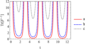
Figure 1: (Color online) Total precision limit, given by Eq. (44), as a function of time for $B=1$, $\theta=\pi/2$, and different values of $p_{0}$ ($p_{1}=1-p_{0}$). (a) $p_{0}=1$ (solid-red line). (b) $p_{0}=0.8$ (dashed-blue line). (c) $p_{0}=0.6$ (dot-dashed-gray line).

III QFI of a unitary process with two different parametrizations

Let us consider a unitary transformation parameterized in terms of two different classes of parameters $\bm{\alpha}=\{\alpha_{k}\}$ and $\bm{\beta}=\{\beta_{l}\}$, i.e. $U(\bm{\alpha})=U(\bm{\beta})$. Now the question is that if we start with the same initial state $\rho_{0}$ and encode these parameters on the state as

$$\rho_{\bm{\alpha}} = U(\bm{\alpha})\rho_{0}U^{\dagger}(\bm{\alpha})$$

$$= U(\bm{\beta})\rho_{0}U^{\dagger}(\bm{\beta})=\rho_{\bm{\beta}},$$

what is the relation between the QFI matrices of these two parametrizations?

To address this question we should first find a relation between $M$-matrices with respect to these classes of parameters. To do so, we write Eq. (5) for $\alpha_{k}$ and $\beta_{l}$ as ${M}_{\alpha_{k}}=iU^{\dagger}\frac{\partial U}{\partial{\alpha_{k}}}$ and ${M}_{\beta_{l}}=iU^{\dagger}\frac{\partial U}{\partial{\beta_{l}}}$, respectively. By using $\frac{\partial U}{\partial\beta_{l}}=\sum_{k}\frac{\partial U}{\partial\alpha_{k}}\frac{\partial\alpha_{k}}{\partial\beta_{l}}$, we get

$${M}_{\beta_{l}}=i\sum_{k}U^{\dagger}\frac{\partial U}{\partial\alpha_{k}}\frac{\partial\alpha_{k}}{\partial\beta_{l}}=\sum_{k}M_{\alpha_{k}}S_{\alpha_{k},\beta_{l}},$$ (46)

where we have defined the transfer matrix $S$ with matrix elements $S_{\alpha_{k},\beta_{l}}=\frac{\partial\alpha_{k}}{\partial\beta_{l}}$. Similarly, if we write Eq. (16) for $\alpha_{k}$ and $\beta_{l}$ and by using Eq. (46) we find a relation between SLD matrices with respect to these classes of parameters

$$\left(L_{\beta_{l}}\right)_{\tilde{a}\tilde{b}}=\sum_{k}\left(L_{\alpha_{k}}\right)_{\tilde{a}\tilde{b}}S_{\alpha_{k},\beta_{l}}.$$ (47)

Finally the relation between various parametrizations of the QFI can be expressed by

$$F_{{\beta_{l}}{\beta_{l^{\prime}}}}=\sum_{k}\sum_{k^{\prime}}S_{\alpha_{k},\beta_{l}}F_{{\alpha_{k}}{\alpha_{k^{\prime}}}}S_{\alpha_{k^{\prime}},\beta_{l^{\prime}}},$$ (48)

which can be written in a more compact form as

$$F^{\{\beta_{l}\}}=S^{\mathrm{t}}F^{\{\alpha_{k}\}}S.$$ (49)

Very recently a similar relation is presented in Ref. GoldbergPRA2018 , however it is for the special case of $SU(2)$ processes with the aim of calculating the QFI of arbitrary parameters of $SU(2)$ using the one of the Euler angles. Regarding this, Eq. (48) is general in a sense that it enables one to obtain the QFI matrix of an arbitrary unitary process for a given set of estimation parameters from the one of the other set of parameters, with no restriction on the number of the initial and final estimation parameters.

For the simplest case of $SU(2)$ processes, the relation between QFI of different parametrizations can be expressed in terms of a relation between $\bm{m}$-vectors of the corresponding parameters. Actually, if $\bm{m}_{\alpha_{k}}$ and $\bm{m}_{\beta_{l}}$ denote the $\bm{m}$-vectors of a unitary process in the $\{\alpha_{k}\}$ and $\{\beta_{l}\}$ parametrizations, respectively, we find from Eq. (46)

$${\bm{m}}_{\beta_{l}}=\sum_{k}\bm{m}_{\alpha_{k}}S_{\alpha_{k},\beta_{l}}.$$ (50)

In view of this, both $F_{\alpha_{k}\alpha_{k^{\prime}}}$ and $F_{\beta_{l}\beta_{l^{\prime}}}$ are given by the same relation (1) with their own $\bm{m}$-vectors replaced by $\bm{m}_{\theta_{i}}$. In order to show how the above algorithm works, in the example below we will obtain the QFI of a unitary process in the coset representation from the one in the canonical representation.

Example.—Consider again a system described by the Hamiltonian (22) and parametrization (28). The unitary evolution generated by this Hamiltonian provides the canonical mapping of the algebra onto the group GilmoreBook2012 . On the other hand, an arbitrary unitary matrix $U\in SU(2)$ can be written in a unique way as a product of two group elements GilmoreBook2012

$$U(\eta,\gamma,\xi)=\Omega^{\left(2\right)}(\gamma,\xi)\Omega^{\left(1\right)}(\eta),$$ (51)

where $\Omega^{\left(1\right)}(\eta)=\exp\{-i\eta\sigma_{z}/2\}$ is diagonal (in the computational basis $\{|0\rangle,|1\rangle\}$), corresponding to the one-dimensional Cartan subalgebra of $su(2)$, and $\Omega^{\left(2\right)}(\gamma,\xi)=\exp\{-i\gamma(\sigma_{x}\sin{\xi}+\sigma_{y}\cos{\xi})/2\}$ is an arbitrary element of the two-dimensional quotient space $S^{2}=SU(2)/U(1)$. The relation between the canonical parameters $\{r,\vartheta,\varphi\}$ and the aim parameters $\{\eta,\gamma,\xi\}$ is

$$r = \frac{1}{t}\cos^{-1}\left(\cos{\frac{\gamma}{2}}\cos\frac{\eta}{2}\right),$$ (52)

$$\vartheta = \cos^{-1}\left(\frac{\cos{\frac{\gamma}{2}}\sin{\frac{\eta}{2}}}{\sqrt{1-\cos^{2}{\frac{\gamma}{2}}\cos^{2}{\frac{\eta}{2}}}}\right),$$ (53)

$$\varphi = \tan^{-1}\left(\cot\left(\xi+\frac{\eta}{2}\right)\right),$$ (54)

which can be used to calculate the transfer matrix $S$. After calculating $S$, and regarding that we have an explicit expression for $\bm{m}$-vectors in the parameters $\{r,\vartheta,\varphi\}$, Eq (33), one can invoke Eq. (50) and get

$${\bm{m}_{\eta}} = \frac{1}{2}\left(0,0,1\right)^{\mathrm{t}},$$ (55)

$${\bm{m}_{\gamma}} = \frac{1}{2}\left(\sin\Gamma,\cos\Gamma,0\right)^{\mathrm{t}},$$ (56)

$${\bm{m}_{\xi}} = \sin{\frac{\gamma}{2}}\left(\cos\frac{\gamma}{2}\cos\Gamma,-\cos\frac{\gamma}{2}\sin\Gamma,-\sin\frac{\gamma}{2}\right)^{\mathrm{t}},$$ (57)

where $\Gamma=\xi+\eta$. Having these $\bm{m}$-vectors in hand, one can easily use Eq. (1) to calculate QFI of the coset parameters for an arbitrary initial state. For instance, when the initial state is diagonal in the computational basis $\{|0\rangle,|1\rangle\}$, we get

$$F(\eta,\gamma,\xi)=(p_{0}-p_{1})^{2}\begin{pmatrix}0&0&0\\ 0&1&0\\ 0&0&\sin^{2}{\gamma}\end{pmatrix}.$$ (58)

This simple form for $F(\eta,\gamma,\xi)$, in particular vanishing $F_{\eta\eta}(\eta,\gamma,\xi)$, is not surprising as we have assumed that $\rho_{0}$ is diagonal in the Cartan basis of the algebra, so that $\rho$ cannot encode any parameters of the Cartan subalgebra.

IV Conclusion

In this paper, we have considered the quantum Fisher information for unitary processes with special attention to $SU(2)$ processes. In particular, we have presented a new formulation to calculate QFI matrix in terms of vectors $\bm{m}_{\theta_{i}}\in\mathbb{R}^{3}$, associated to each estimation parameter $\theta_{i}$. Our method gives a closed relation for the QFI matrix and reveals, simply, its features. Furthermore, for a general Hamiltonian with arbitrary parametrization, we have provided a closed relation to calculate vectors $\bm{m}_{\theta_{i}}$. The relation is expressed in terms of derivatives of the Hamiltonian parameters with respect to the parameters under estimation. As an application we choose angle-axis parameters, both as Hamiltonian parametrization and estimation parameters, and calculate QFI. The generalization of the method to dimensions higher than two is not straightforward and is under further consideration.

Finally, using a linear transformation between two different parameter spaces of a unitary process, we find a relation between QFI matrices of two different classes of estimation parameters. This can be used, in particular, to calculate the QFI of a unitary process in terms of the one of the same process but with different parametrization, provided that the linear transformation between two parameter spaces is known. For illustration, we have applied this method for a spin-half system and obtained the QFI matrix of the coset parameters in terms of the one of the angle-axis parameters.

- (1) Giovannetti, V., Lloyd, S., Maccone, L.: Quantum-enhanced measurements: beating the standard quantum limit. Science 306, 1330-1336 (2004)
- (2) Giovannetti, V., Lloyd, S., Maccone, L.: Advances in quantum metrology. Nat. Photonics 5, 222-229 (2011)
- (3) Huang, J., Wu, S., Zhong, H., Lee, C.: Quantum Metrology With Cold Atoms. Annual Review of Cold Atoms and Molecules 2, 365-415 (2014)
- (4) Georgescu, I.: Quantum technology: The golden apple. Nat. Phys. 10, 474 (2014)
- (5) Giorda, P., Paris, M.G.A.: Gaussian Quantum Discord. Phys. Rev. Lett. 105, 020503 (2010)
- (6) Ollivier, H., Zurek, W. H.: Quantum Discord: A Measure of the Quantumness of Correlations. Phys. Rev. Lett. 88, 017901 (2001)
- (7) Braginsky, V., Vyatchanin, S.: Corner reflectors and quantum-non-demolition measurements in gravitational wave antennae. Phys. Lett. A 324, 345-360 (2004)
- (8) Adhikari, R.X.: Gravitational radiation detection with laser interferometry. Rev. Mod. Phys. 86, 121 (2014)
- (9) McGuirk, J. M., Foster, G.T., Fixler, J.B., Snadden, M.J., Kasevich, M.A.: Sensitive absolute-gravity gradiometry using atom interferometry. Phys. Rev. A 65, 033608 (2002)
- (10) Santarelli, G., Laurent, P., Lemonde, P.,Clairon, A., Mann, A.G., Chang, S., Luiten, A.N., Salomon, C.: Quantum Projection Noise in an Atomic Fountain: A High Stability Cesium Frequency Standard. Phys.Rev. Lett. 82, 4619 (1999)
- (11) Bollinger, J.J., Itano, W.M., Wineland, D.J., Heinzen, D.J.: Optimal frequency measurements with maximally correlated states. Phys. Rev. A 54, R4649 (1996)
- (12) Huelga, S.F., Macchiavello, C., Pellizzari, T., Ekert, A.K., Plenio, M.B., Cirac, J.I.: Improvement of frequency standards with quantum entanglement. Phys. Rev. Lett. 79, 3865 (1997)
- (13) Tsang, M.: Quantum Imaging beyond the Diffraction Limit by Optical Centroid Measurements. Phys. Rev. Lett. 102, 253601 (2009)
- (14) Giovannetti, V., Lloyd, S., Maccone, L., Shapiro, J.H.: Sub-Rayleigh-diffraction-bound quantum imaging. Phys. Rev. A 79, 013827 (2009)
- (15) Brida, G., Genovese, M., Berchera, I.R.: Experimental realization of sub-shot-noise quantum imaging. Nat. Photonics 4, 227-230 (2010)
- (16) Bužek, V., Derka, R., Massar, S.: Optimal Quantum Clocks. Phys. Rev. Lett. 82, 2207 (1999)
- (17) André, A., Sørensen, A.S., Lukin, M.D.: Stability of Atomic Clocks Based on Entangled Atoms. Phys. Rev. Lett. 92, 230801 (2004)
- (18) Louchet-Chauvet, A., Appel, J., Renema, J.J., Oblak, D., Kjaergaard, N., Polzik, E.S.: Entanglement-assisted atomic clock beyond the projection noise limit. New J. Phys. 12, 065032 (2010)
- (19) Borregaard, J., Sørensen, A.S.: Near-Heisenberg-Limited Atomic Clocks in the Presence of Decoherence. Phys. Rev. Lett. 111, 090801 (2013)
- (20) Kessler, E.M., Kómár, P., Bishof, M., Jiang, L., Sørensen, A.S., Ye, J., Lukin, M.D.: Heisenberg-Limited Atom Clocks Based on Entangled Qubits. Phys. Rev. Lett. 112, 190403 (2014)
- (21) Holevo, A.S.: Probabilistic and Statistical Aspects of Quantum Theory. North-Holland, Amsterdam (1982)
- (22) Helstrom, C.W.: Quantum Detection and Estimation Theory. Academic, New York (1976)
- (23) Braunstein, S.L., Caves, C.M.: Statistical distance and the geometry of quantum states. Phys. Rev. Lett. 72, 3439 (1994)
- (24) Braunstein, S.L., Caves, C.M., Milburn, G.J.: Generalized uncertainty relations: theory, examples, and Lorentz invariance. Ann. Phys. (N.Y.) 247, 135-173 (1996)
- (25) Petz, D.: Covariance and Fisher information in quantum mechanics. J. Phys. A: Math. Gen. 35, 929 (2002)
- (26) Petz, D.: Quantum Information Theory and Quantum Statistics. Springer, Berlin (2008)
- (27) Giovannetti, V., Lloyd, S., Maccone, L.: Quantum metrology. Phys. Rev. Lett. 96, 010401 (2006)
- (28) Lee, C.: Adiabatic Mach-Zehnder Interferometry on a Quantized Bose-Josephson Junction. Phys. Rev. Lett. 97, 150402 (2006)
- (29) Pezzé, L., Smerzi, A.: Entanglement, Nonlinear Dynamics, and the Heisenberg Limit. Phys. Rev. Lett. 102, 100401 (2009)
- (30) Fisher, R.A.: Theory of Statistical Estimation. Proc. Cambridge Philos. Soc. 22, 700 (1925)
- (31) Bures, D.: An extension of Kakutaniś thoerm on infinite product measures to the tensor product of semifinite w*-algebras. Trans. Amer. Math. Soc. 135, 199-212 (1969)
- (32) Uhlmann, A.: Parallel transport and ”quantum holonomy” along density operators. Rep. Math. Phys. 24, 229 (1986)
- (33) Hübner, M.: Explicit computation of the Bures distance for density matrices. Phys. Lett. A 163, 239-242 (1992)
- (34) Luo, S., Zhang, Q.: Informational distance on quantum-state space. Phys. Rev. A 69, 032106 (2004)
- (35) Sarovar, M., Milburn, G.: Optimal estimation of one-parameter quantum channels. J. Phys. A: Math. Gen. 39, 8487 (2006)
- (36) Monras, A., Paris, M.G.A.: Optimal quantum estimation of loss in bosonic channels. Phys. Rev. Lett. 98, 160401 (2007)
- (37) Watanabe, Y., Sagawa, T., Ueda, M.: Optimal measurement on noisy quantum systems. Phys. Rev. Lett. 104, 020401 (2010)
- (38) Lu, X., Wang, X., Sun, C.P.: Quantum Fisher information flow and non-Markovian process of open systems. Phys. Rev. A 82, 042103 (2010)
- (39) Escher, B.M., de Matos Filho, R.L., Davidovich, L.: General framework for estimating the ultimate precision limit in noisy quantum-enhanced metrology. Nat. Phys. 7, 406-411 (2011)
- (40) Ma, J., Huang, Y., Wang, X., Sun, C.P.: Quantum Fisher information of the Greenberger-Horne-Zeilinger state in decoherence channels. Phys. Rev. A 84, 022302 (2011)
- (41) Chin, A.W., Huelga, S.F., Plenio, M.B.: Quantum metrology in non-Markovian environments. Phys. Rev. Lett. 109, 233601 (2012)
- (42) Berrada, K., Abdel-Khalek, S., Obada, A.-S.F.: Quantum Fisher information for a qubit system placed inside a dissipative cavity. Phys. Lett. A 376, 1412-1416 (2012)
- (43) Zhong, W., Sun, Z., Ma, J., Wang, X., Nori, F.: Fisher information under decoherence in Bloch representation. Phys. Rev. A 87, 022337 (2013)
- (44) Berrada, K.: Non-Markovian effect in the precision of parameter estimation. Phys. Rev. A 88, 035806 (2013)
- (45) Ozaydin, F.: Phase damping destroys quantum Fisher information of W states. Phys. Lett. A 378, 3161-3164 (2014)
- (46) Alipour, S., Mehboudi, M., Rezakhani, A.T.: Quantum metrology in open systems: dissipative Cram’er-Rao bound. Phys. Rev. Lett. 112, 120405 (2014)
- (47) Ban, M.: Quantum Fisher information of a qubit initially correlated with a non-Markovian environment. Quantum Inf. Process. 14, 11, 4163-4177 (2015)
- (48) Pang, S., Brun, T.A.: Quantum metrology for a general Hamiltonian parameter. Phys. Rev. A 90, 022117 (2014)
- (49) Liu, J., Xiong, H.-N., Song, F., Wang, X.: Fidelity susceptibility and quantum Fisher information for density operators with arbitrary ranks. Physica A: Stat. Mech. App. 410, 167 (2014)
- (50) Liu, J., Jing, X.-X., Zhong, W., Wang, X.-G.: Quantum Fisher Information for Density Matrices with Arbitrary Ranks. Commun. Theor. Phys. 61, 45 (2014)
- (51) Liu, J., Jing, X.-X., Wang, X.: Quantum metrology with unitary parametrization processes. Sci. Rep. 5, 8565, (2015)
- (52) Jing, X.-X., Liu, J., Xiong, H.-N., Wang, X.: Maximal quantum Fisher information for general su(2) parametrization processes. Phys. Rev. A 92, 012312 (2015)
- (53) Boixo, S., Flammia, S.T., Caves, C.M., Geremia, J.: Generalized Limits for Single-Parameter Quantum Estimation. Phys. Rev. Lett. 98, 090401 (2007)
- (54) Taddei, M.M., Escher, B.M., Davidovich, L., de Matos Filho, R.L.: Quantum Speed Limit for Physical Processes. Phys. Rev. Lett. 110, 050402 (2013)
- (55) Suzuki, J.: Parameter estimation of qubit states with unknown phase parameter. Int. J. Quant. Inf. 13, 1450044 (2015)
- (56) Suzuki, J.: Explicit formula for the Holevo bound for two-parameter qubit-state estimation problem. J. Math. Phys. 57, 042201 (2016)
- (57) Wilcox, R.M.: Exponential Operators and Parameter Differentiation in Quantum Physics. J. Math. Phys. 8, 962 (1967)
- (58) Goldberg, A.Z., James, D.F.V.: Quantum-limited Euler angle measurements using anticoherent states. Phys. Rev. A 98, 032113 (2018)
- (59) Gilmore, R.: Lie groups, Lie algebras, and some of their applications. Courier Corporation, (2012)