Analytic continuation of the kite family

Abstract

We consider results for the master integrals of the kite family, given in terms of ELi-functions which are power series in the nome $q$ of an elliptic curve. The analytic continuation of these results beyond the Euclidean region is reduced to the analytic continuation of the two period integrals which define $q.$ We discuss the solution to the latter problem from the perspective of the Picard-Lefschetz formula.

1 Introduction

In this talk, we consider the family of Feynman integrals associated to the kite graph, shown in fig. 1 (c). Certain master integrals of this family have recently served as interesting showcases for the problem that multiple polylogarithms are not always sufficient to express the coefficients of Feynman integrals in the Laurent expansion in $\epsilon$ of dimensional regularization. Elliptic generalizations of (multiple) polylogarithms can be used to express these integrals instead. In AdaBogSchWei a way to recursively obtain the master integrals of this family to arbitrary order in $\epsilon$ was presented for the Euclidean kinematic region. This computation and previous related work on the sunrise integral AdaBogWei1 ; AdaBogWei2 ; AdaBogWei3 ; AdaBogWei4 rely crucially on properties of an underlying elliptic curve and its periods, which were pointed out in BloVan . The results for the master integrals of the kite family are expressed in terms of a class of functions defined in AdaBogWei4 as power series in the nome $q$ of this elliptic curve. Alternative expressions in terms of iterated integrals of modular forms were found in AdaWei and results for the first order of the Laurent expansion were previously derived in RemTan2 .

Here we focus on the analytic continuation of the results for the kite family BogSchWei beyond the Euclidean region. By considering the periods of the underlying elliptic curve, we can reduce the analytic continuation of the Feynman integrals to the question how cycles on the elliptic curve behave under the variation of a kinematic invariant. The answer to this question is then very simple and can be deduced from an application of the Picard-Lefschetz formula Lef , as we want to emphasise with this presentation. In this way we arrive at analytic results for the master integrals which can be evaluated numerically at any real value of the kimematic invariant, the singular points being the only exceptions.

Under certain conditions, which are met in our problem, the Picard-Lefschetz formula determines the variation undergone by integration domains when an unintegrated variable of the integral is sent on a path in the complex plane around a value, where a pinch singularity of the integral occurs. It was known for a long time that at least in some well behaved cases, the formula would apply to Feynman integrals and predict their analytic structure. With this motivation in mind, the theory was extended by Fotiadi, Froissart, Lascoux and especially by Pham Fotetal ; Pha1 ; Pha2 in the sixties, using results of Thom Tho and Leray Ler . Related literature from the sixties and seventies shows that already for rather simple Feynman integrals a practical application of Picard-Lefschetz theory is far from trivial.

Since then, other methods to determine the analytic properties of Feynman integrals have become more important. Cutkosky rules predict the discontinuities in a handy, graphical way in terms of cut-integrals. Furthermore, if the Feynman integral can be computed in the Euclidean region in terms of sufficiently well-known functions such as multiple polylogarithms, the analytic continuation to other regions can be deduced from the analytic properties of these functions. However, the mentioned theory framework around the Picard-Lefschetz theorem seems to experience new attention in the recent literature on Feynman integrals. Extended Picard-Lefschetz theory was used in a recent proof of the Cutkosky rules in BloKre . Furthermore, in a series of articles Abretal1 ; Abretal2 ; Abretal3 which employs Leray’s residue theory for the definition of cut integrals, it is suggested that the discontinuities play a crucial role in a conjectured co-product structure on Feynman integrals, motivated from the co-product on polylogarithms. We take these recent developments as additional motivation to emphasise the role of homology in our application.

Our presentation is organized as follows: In the next section, we review the family of Feynman integrals associated to the kite graph and its underlying family of elliptic curves. In section 3 we reduce the problem of the analytic continuation of the master integrals of the kite family to the question how the periods of the elliptic curve behave under a particular variation of a kinematic parameter. Section 4 discusses the latter problem as an application of the Picard-Lefschetz formula.

2 The kite family and its elliptic curve

We consider the family of Feynman integrals associated to the kite graph of fig. 1 (c). The same particle mass $m$ is assigned to each of the three solid internal edges while the propagators drawn with dashed lines are massless. The graph has one external momentum $p$ and we define $t=p^{2}.$ The integrals of this family in $D$-dimensional Minkowski space are

$$I\left(\nu_{1},\nu_{2},\nu_{3},\nu_{4},\nu_{5}\right)=(-1)^{\nu}\int\frac{d^{D}l_{1}d^{D}l_{2}}{\left(i\pi^{\frac{d}{2}}\right)^{2}}\prod_{i=1}^{5}D_{i}^{-\nu_{i}}$$

with inverse propagators $D_{1}=l_{1}^{2}-m^{2},\,D_{2}=l_{2}^{2},\,D_{3}=(l_{1}-l_{2})^{2}-m^{2},\,D_{4}=(l_{1}-p)^{2},\,D_{5}=(l_{2}-p)^{2}-m^{2}$ and $\nu=\sum_{i=1}^{5}\nu_{i}.$ The integration is over loop-momenta $l_{1},l_{2}.$ These integrals are obviously functions of $D,t$ and $m^{2}$ which is suppressed in our notation. By integration-by-parts reduction, the integrals of this family with $\nu_{i}\in\mathbb{Z}$ can be expressed as linear combinations of eight master integrals, which can be chosen as $I(2,0,2,0,0),$ $I(2,0,2,1,0),$ $I(0,2,2,1,0),$ $I(0,2,1,2,0),$ $I(2,1,0,1,2),$ $I(1,0,1,0,1),$ $I(2,0,1,0,1),$ $I(1,1,1,1,1).$ The first five of these integrals can be expressed in terms of multiple polylogarithms Gon2 ; Gon1

$$\textrm{Li}_{n_{1},...,n_{r}}(z_{1},...,z_{r})=\sum_{j_{1}>j_{2}>...>j_{r}>0}\frac{z_{1}^{j_{1}}...z_{r}^{j_{r}}}{j_{1}^{n_{1}}...j_{r}^{n_{r}}}\textrm{ for }\left|z_{i}\right|<1.$$

The latter three integrals correspond to the graphs in fig. 1 respectively. For the computation of these inegrals, multiple polylogarithms are not sufficient. In particular the sunrise integral $I(1,0,1,0,1)$ has been essential in recent developments to extend the classes of functions applied in Feynman integral computations beyond multiple polylogarithms. We refer to Abletal ; AdaChaWei1 ; AdaChaWei2 ; AdaWei2 ; BloKerVan1 ; BloKerVan2 ; BroDuhetal1 ; BroDuhetal2 ; BroDuhetal3 ; Broe1 ; Bro2 ; Bro3 ; Bro4 ; ManTan ; PriTan ; PriTan2 ; RemTan3 for some of these recent developments in quantum field theory and string theory.

The master integrals of the kite family can be computed by use of the method of differential equations, deriving a system of ordinary first-order differential equations in the variable $t.$ It was shown in AdaBogSchWei ; RemTan2 that certain changes of the basis of master integrals simplifies the system of equations and in AdaWei2 it was shown that by a non-algebraic change of variables, the system can even be written in canonical form Hen2 . Results for the master integrals were given in terms of elliptic generalizations of (multiple) polylogarithms. In AdaBogSchWei it was shown that in the Euclidean region where $t<0$ the master integrals can be expressed in terms of functions

$$\textrm{ELi}_{n;m}(x;y;q)=\sum_{j=1}^{\infty}\sum_{k=1}^{\infty}\frac{x^{j}}{j^{n}}\frac{y^{k}}{k^{m}}q^{jk}=\sum_{k=1}^{\infty}\frac{y^{k}}{k^{m}}\textrm{Li}_{n}(q^{k}x),$$ (1)

and multi-variable generalizations

$$\textrm{ELi}_{n_{1},...,n_{l};m_{1},...,m_{l};2o_{1},...,2o_{l-1}}\left(x_{1},...,x_{l};y_{1},...,y_{l};q\right)$$

$$=\sum_{j_{1}=1}^{\infty}...\sum_{j_{l}=1}^{\infty}\sum_{k_{1}=1}^{\infty}...\sum_{k_{l}=1}^{\infty}\frac{x_{1}^{j_{1}}}{j_{1}^{n_{1}}}...\frac{x_{l}^{j_{l}}}{j_{l}^{n_{l}}}\frac{y_{1}^{k_{1}}}{k_{1}^{m_{1}}}..\frac{y_{l}^{k_{l}}}{k_{l}^{m_{l}}}\frac{q^{j_{1}k_{1}+...+j_{l}k_{l}}}{\prod_{i=1}^{l-1}\left(j_{i}k_{i}+...+j_{l}k_{l}\right)^{o_{i}}}$$ (2)

to all orders in $\epsilon=(4-D)/2.$ Results in terms of iterated integrals over modular forms were derived in AdaWei . For the purpose of this presentation, aiming at the analytic continuation of the results beyond the Euclidean region, the precise shape of the results for the master integrals is not relevant. The following discussion merely uses the fact that up to simple prefactors the results can be expressed as power series in $q=q(t)$ which is the nome of a family of elliptic curves, with the parameter of the family being the kinematic invariant $t.$

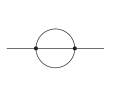
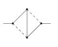
(a)                                         (b)                                        (c)

Figure 1: The sunrise graph (a), the sunrise with one raised index (b), and the kite graph (c).

This family of elliptic curves is derived from the sunrise integral $I(1,0,1,0,1)$ following BloVan . The second Symanzik polynomial reads

$$\mathcal{F}=-x_{1}x_{2}x_{3}t+m^{2}\left(x_{1}+x_{2}+x_{3}\right)\left(x_{1}x_{2}+x_{2}x_{3}+x_{1}x_{3}\right).$$

A change of variables transforms the equation $\mathcal{F}=0$ to the Weierstrass normal form

$$y^{2}=4\left(x-e_{1}\right)\left(x-e_{2}\right)\left(x-e_{3}\right)$$

with the three roots

$$e_{1} = \frac{1}{24}\left(-t^{2}+6m^{2}t+3m^{4}+3\left(m^{2}-t\right)^{\frac{3}{2}}\left(9m^{2}-t\right)^{\frac{1}{2}}\right)$$

$$e_{2} = \frac{1}{24}\left(-t^{2}+6m^{2}t+3m^{4}-3\left(m^{2}-t\right)^{\frac{3}{2}}\left(9m^{2}-t\right)^{\frac{1}{2}}\right)$$

$$e_{3} = \frac{1}{24}\left(2t^{2}-12m^{2}t-6m^{4}\right)$$

of the cubical polynomial in $x,$ satisfying $e_{1}+e_{2}+e_{3}=0.$ The family of elliptic curves degenerates at the values $0,\,m^{2},\,9m^{2},\,\infty$ of the parameter $t.$ In the Euclidean region $t<0$ the three roots are real and separated as $e_{1}>e_{3}>e_{2}$. Here we define the period integrals

$$\psi_{1}=2\int_{e_{2}}^{e_{3}}\frac{dx}{y},\;\psi_{2}=2\int_{e_{1}}^{e_{3}}\frac{dx}{y}$$

which evaluate to

$$\psi_{1}=\frac{4}{\left(m^{2}-t\right)^{\frac{3}{4}}\left(9m^{2}-t\right)^{\frac{1}{4}}}K(k),\;\psi_{2}=\frac{4i}{\left(m^{2}-t\right)^{\frac{3}{4}}\left(9m^{2}-t\right)^{\frac{1}{4}}}K(k^{\prime})$$

with the complete elliptic integral of the first kind

$$K(k)=\int_{0}^{1}\frac{dt}{\sqrt{\left(1-t^{2}\right)\left(1-k^{2}t^{2}\right)}}$$ (3)

where the modulus $k$ and the complementary modulus $k^{\prime}$ are given by

$$k=\frac{e_{3}-e_{2}}{e_{1}-e_{2}},\;k^{\prime 2}=1-k^{2}=\frac{e_{1}-e_{3}}{e_{1}-e_{2}}.$$

With these periods we introduce

$$\tau=\frac{\psi_{2}}{\psi_{1}},\,\,\,q=e^{i\pi\tau}.$$

The mentioned results of AdaBogSchWei for the eight master integrals in the Euclidean are expressed in terms of the functions of eqs. 1 and 2 with the nome $q.$ Up to simple general prefactors involving the first period $\psi_{1},$ this is their only dependence of the kinematic invariant $t.$

3 Analytic continuation

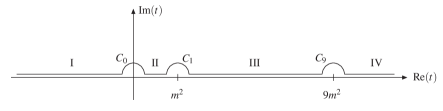
Figure 2: Variation contour in the complex $t$-plane.

The previous section has shown that the analytic continuation of the eight master integrals of the kite family can be reduced to the analytic continuation of the two period integrals $\psi_{1},\psi_{2}.$ We are interested in the analytic behaviour of the periods $\psi_{1},\psi_{2}$ as $t$ varies along the real axis beyond the Euclidean region. As singular points and branch cuts of the period integrals correspond to real values of $t,$ we consider the variation of $t$ in the complex $t$-plane and shift the contour of this variation slightly away from the real axis by Feynman’s prescription $t\rightarrow t+i\delta.$ Here $\delta$ is small, real, positive and sent to zero in the end for evaluations on the real axis. We choose the contour such that it furthermore circumvents the singular points in small half circles. Fig. 2 shows the contour of the variation of $t.$

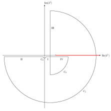
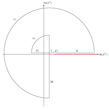
Figure 3: Variations in the complex plane of $k^{2}$ and $k^{\prime 2}.$

In order to discuss the branch cut behaviour of the periods, it is furthermore useful to consider the complete elliptic integral of the first kind in eq. 3 as a function of $k^{2}$ and note that it has only one branch cut $[1,\infty[$ in the complex $k^{2}$-plane. We study the question, where along the variation of $t$ this branch cut is crossed for the two periods. Fig. 3 shows the behaviour of $k^{2}$ and $k^{\prime 2}$ as $t$ is varied along the contour of fig. 2. We notice that $k^{\prime 2}$ does not cross the branch cut of the complete elliptic integral at all. The variable $k^{2}$ crosses the branch cut only once. This happens as $t$ is varied on the half circle $C_{1}$ around the singular point $t=m^{2}.$ Therefore it is this piece of the contour of $t$ along which we have to study the behaviour of the first period $\psi_{1}$ more closely.

The three quarters of the circle which $k^{2}$ takes in fig. 3 may be deformed to a full circle for convenience. In order to study this variation, we consider the Legendre form

$$y^{2}=x(x-\lambda)(x-1)$$

of the family of elliptic curves, where $\lambda=k^{2}.$ As $t$ varies along $C_{1},$ the parameter $\lambda$ moves in a small circle around $1.$ Equivalently, we can describe this variation by

$$y^{2}=x(x-e_{1}(\varphi))(x-e_{2}(\varphi))$$

with $e_{1}(\varphi)=1-re^{i\varphi},\,\,\,\,\,e_{2}(\varphi)=1+re^{i\varphi}$ where $r$ is a small, positive, real number and $\varphi$ is an angle whose value is 0 in the beginning and monotonously rises to $2\pi.$ In order to observe the change of the two periods along this variation, it is convenient to write them as integrals over cycles $\delta_{1},\delta_{2}$ which form a basis of the first homology group of the elliptic curve. We introduce

$$P_{1}(\varphi)=\int_{\delta_{1}}\frac{dx}{y},\,\,\,P_{2}(\varphi)=\int_{\delta_{2}}\frac{dx}{y},\,\,\,y=-\sqrt{x}\sqrt{x-e_{1}(\varphi)}\sqrt{x-e_{2}(\varphi)},$$

where the cycles $\delta_{1},\delta_{2}$ are oriented such that

$$P_{1}(0)=2\int_{0}^{e_{1}(0)}\frac{dx}{y}=-2\int_{e_{2}(0)}^{\infty}\frac{dx}{y}\,\,\,\textrm{ and \,\,\,}P_{2}(0)=2\int_{e_{2}(0)}^{e_{1}(0)}\frac{dx}{y}$$

with the integration contour on the right-hand side slightly shifted by a negative imaginary part for $x.$

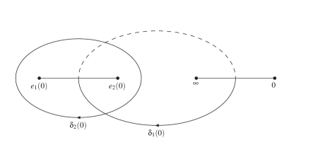
Figure 4: The cycles $\delta_{1}$ and $\delta_{2}$ before the variation.

Fig. 4 shows the cycles $\delta_{1},\delta_{2}$ on the elliptic curve. The use of dashed and straight lines indicates that $\delta_{1}$ has two parts in two different Riemann sheets of the elliptic curve, separated by the branch cuts. The question is: How do the two cycles change under the mentioned variation? This will be discussed in section 4. There we will see that $\delta_{1}$ becomes $\delta_{1}-2\delta_{2}$ while $\delta_{2}$ remains unchanged. We therefore obtain:

$$P_{1}(2\pi)=P_{1}(0)-2P_{2}(0)\,\,\,\textrm{and}\,\,\,P_{2}(2\pi)=P_{2}(0).$$

This is the behaviour of the periods as $t$ varies around the critical point $t=m^{2}.$ The above discussion has shown that the behaviour along all other pieces of the variation is trivial. We hence arrive at the analytic continuation of the two period integrals:

$$\left(\begin{array}[]{c}\psi_{2}(t+i\delta)\\ \psi_{1}(t+i\delta)\end{array}\right)=\frac{4}{\left(m^{2}-t-i\delta\right)^{\frac{3}{4}}\left(9m^{2}-t-i\delta\right)^{\frac{1}{4}}}M_{t}\left(\begin{array}[]{c}iK\left(k^{\prime}\left(t+i\delta\right)\right)\\ K\left(k\left(t+i\delta\right)\right)\end{array}\right)$$

with

$$M_{t}=\begin{cases}\left(\begin{array}[]{cc}1&0\\ 0&1\end{array}\right)&\textrm{ for }-\infty<t<m^{2},\\ \left(\begin{array}[]{cc}1&0\\ -2&1\end{array}\right)&\textrm{ for }m^{2}<t<\infty.\end{cases}$$

Applying this result in terms of

$$q(t+i\delta)=e^{i\pi\frac{\psi_{2}(t+i\delta)}{\psi_{1}(t+i\delta)}}$$

to the functions in eqs. 1 and 2, we obtain the analytic continuation of the results for the master integrals of the kite family. As an example, the results for the $\epsilon^{0}$-term for the kite integral $I(1,1,1,1,1)$ in $4-2\epsilon$ dimensions is plotted in fig. 5.

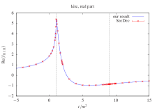
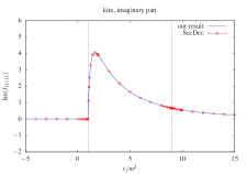
Figure 5: The real and imaginary parts of the $\epsilon^{0}$-term of the kite integral. The dashed vertical lines indicate $t=m^{2}$ and $t=9m^{2}.$ The blue line is our analytic result and the red dots are numerical data produced with the program SecDec Boretal .

4 An application of the Picard-Lefschetz formula

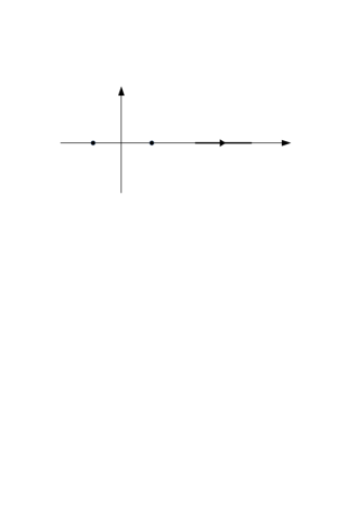
(a)                                                            (b)

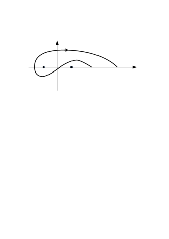
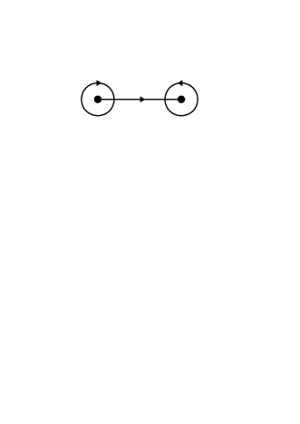
(c)                                                               (d)

Figure 6: Contours in the complex $x$-plane.

Before we discuss the deformation of $\delta_{1}$ which was left open in the previos section, let us recall the main idea of the Picard-Lefschetz formula with the help of a classical example HwaTep . We consider the integral

$$I(\lambda)=\int_{a}^{b}\frac{1}{x^{2}-\lambda}dx=\frac{1}{2\sqrt{\lambda}}\ln\left(\frac{\left(a+\sqrt{\lambda}\right)\left(b-\sqrt{\lambda}\right)}{\left(a-\sqrt{\lambda}\right)\left(b+\sqrt{\lambda}\right)}\right)$$

with real $b>a>0$ depending on a complex parameter $\lambda$. We are interested in the point $\lambda=0$ where the two singular points $e_{1}=-\sqrt{\lambda}$ and $e_{2}=\sqrt{\lambda}$ coincide. As long as the integration contour from $a$ to $b$ is not in between $e_{1}$ and $e_{2},$ this contour is not trapped when the two singular points approach each other. This is the situation of fig. 6 (a), corresponding to the principal sheet of the logarithm. There is no square-root singularity in this case.

The more interesting situation is shown in fig. 6 (b) where the integration contour is in between the points $e_{1}$ and $e_{2}$ and will be trapped for $\lambda=0.$ (This picture is obtained after sending $\lambda$ in a small circle around $a^{2}$ in anti-clockwise direction.) The situation at $\lambda=0$ is known as a simple pinch and it gives rise to a square-root singularity.

Let us now send $\lambda$ in a small circle around $0$ in anti-clockwise direction. We will call this the variation of $\lambda.$ This causes the points $e_{1}$ and $e_{2}$ to rotate around each other in anti-clockwise direction until they have changed positions. The result of this movement is shown in fig. 6 (c). The integration contour is deformed by this rotation as shown in the figure. Along the variation of $\lambda,$ the integral $I(\lambda)$ picks up a discontinuity, which is an integral with the same integrand and the integration contour given by two small cycles $c_{1},c_{2}$ around $e_{1},e_{2}$ with orientations shown in fig. 6 (d). It is easy to see that these two cycles are in a homological sense the difference between the integration contours of $I(\lambda)$ before and after the variation of $\lambda$.

It is this change of integration contours after variations around a simple pinch which is computed in the Picard-Lefschetz formula. The formula can be written as

$$c\rightarrow c+k\cdot h,$$ (4)

where $c$ is a path or cycle, in our case the contour of integration of $I(\lambda),$ the arrow indicates the change along the variation of $\lambda$, $k$ is an integer and $h$ is another cycle. Both, the integer $k$ and the cycle $h$ are determined from a so-called vanishing cycle associated to the pinch situation. In our simple example, the relevant vanishing cycle is the straight line $s$ oriented from $e_{1}$ to $e_{2}$ as shown in fig. 6 (d). This line is indeed vanishing if $\lambda$ goes to zero and it is a relative cycle in the relative homology of the complex plane modulo the set of points $\{e_{1},e_{2}\}.$ We may consider $s$ as an oriented 1-simplex and obtain its boundary as

$$\partial s=e_{2}-e_{1}.$$ (5)

The last ingredient in the construction of the cycle $h$ is the co-boundary operator $\delta$ of Leray Ler . The co-boundary of an $n$-dimensional cycle can be thought of as an $(n+1)$-dimensional tube wrapped around the cycle. In our case, we only need to construct the co-boundary of a point, which is a small circle around this point with anti-clockwise orientation. We obtain

$$h=\delta\left(\partial s\right)=c_{1}+c_{2}$$

where the minus sign in eq. 5 is reflected in the clockwise orientation of $c_{1}.$

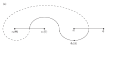
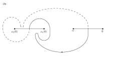
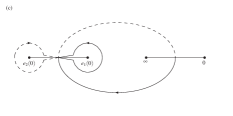
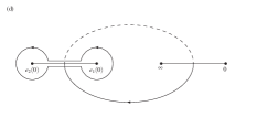
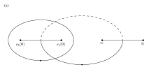
Figure 7: The deformation of $\delta_{1}$ on the elliptic curve.

It remains to determine the integer $k$ in the Picard-Lefschetz formula. Up to a sign, which depends on the dimension of the problem, this number is an intersection number or Kronecker index, depending only on the relative orientation of the cycle $c$ and the vanishing cycle at their intersection. In our case one simply obtains $k=1.$ In conclusion, the Picard-Lefschetz formula predicts $c\rightarrow c+c_{1}+c_{2}$ which is precisely what we have deduced from the figures above.

We are only two steps away from the answer to the question left open in section 3. On the elliptic curve, the points $e_{1}(\lambda),$ $e_{2}(\lambda)$ coincide for $\lambda=1$ and trap the cycle $\delta_{1}$ in a simple pinch, similar to the above example. In contrast to the warm-up example, these two points make not half of a rotation but a full rotation around each other as $\lambda$ is sent around the pinch point. We therefore have an additional factor $2$ in the Picard-Lefschetz formula and obtain

$$\delta_{1}(0)\rightarrow\delta_{1}(2\pi)=\delta_{1}(0)+2\left(c_{1}+c_{2}\right)$$

where $c_{1}$ and $c_{2}$ are the small circles around $e_{1}$ and $e_{2}$ again. The series of snapshots in fig. 7 shows in more detail how after half of a rotation, these circles arise in the deformation of $\delta_{1}$ and from these pictures it is clear, that $c_{1}$ and $c_{2}$ are located in different Riemann sheets. In order to express the change of $\delta_{1}$ in terms of the basis of the first homology group, $\delta_{1}(0),\delta_{2}(0),$ we may pull $c_{1}$ over to the same sheet as $c_{2}.$ This is the step from in fig. 7 (c) to fig. 7 (d). We see that they combine to the cycle $-\delta_{2}(0)$ and arrive at the result

$$\delta_{1}(0)\rightarrow\delta_{1}(2\pi)=\delta_{1}(0)-2\delta_{2}(0)$$

applied in section 3.

We remark that this deformation on the elliptic curve is also a well-known example. Detailed discussions with slightly different visualizations can be found e.g. in Caretal ; Zol where the Riemann sheets, glued together to a torus, are viewed as twisted against each other.

References

- (1) J. Ablinger, J. Blümlein, A. De Freitas, M. van Hoeij, E. Imamoglu, C.G. Raab, C.-S. Radu and C. Schneider, Iterated Elliptic and Hypergeometric Integrals for Feynman Diagrams, arXiv:1706.01299 [hep-th].
- (2) S. Abreu, R. Britto, C. Duhr and E. Gardi, Cuts from residues: the one-loop case, JHEP 1706 (2017) 114, arXiv:1702.03163 [hep-th].
- (3) S. Abreu, R. Britto, C. Duhr and E. Gardi, Algebraic Structure of Cut Feynman Integrals and the Diagrammatic Coaction, Phys. Rev. Lett. 119 (2017) no.5, 051601, arXiv:1703.05064 [hep-th].
- (4) S. Abreu, R. Britto, C. Duhr and E. Gardi, Diagrammatic Hopf algebra of cut Feynman integrals: the one-loop case, JHEP 1712 (2017) 090, arXiv:1704.07931 [hep-th].
- (5) L. Adams, C. Bogner, A. Schweitzer and S. Weinzierl, The kite integral to all orders in terms of elliptic polylogarithms, J. Math. Phys. 57 (2016) 122302, arXiv:1607.01571 [hep-ph].
- (6) L. Adams, C. Bogner, and S. Weinzierl, The two-loop sunrise graph with arbitrary masses, J. Math. Phys. 54 (2013) 052303, arXiv:1302.7004 [hep-ph].
- (7) L. Adams, C. Bogner, and S. Weinzierl, The two-loop sunrise graph in two space-time dimensions with arbitrary masses in terms of elliptic dilogarithms, J. Math. Phys. 55 (2014) 10, 102301,arXiv:1405.5640 [hep-ph].
- (8) L. Adams, C. Bogner, and S. Weinzierl, The two-loop sunrise integral around four space-time dimensions and generalisations of the Clausen and Glaisher functions towards the elliptic case, J. Math. Phys. 56 (2015) no.7, 072303, arXiv:1504.03255 [hep-ph].
- (9) L. Adams, C. Bogner, and S. Weinzierl, The iterated structure of the all-order result for the two-loop sunrise integral, J. Math. Phys. 57 (2016) no.3, 032304, arXiv:1512.05630 [hep-ph].
- (10) L. Adams, E. Chaubey and S. Weinzierl, The planar double box integral for top pair production with a closed top loop to all orders in the dimensional regularisation parameter, arXiv:1804.11144 [hep-ph].
- (11) L. Adams, E. Chaubey and S. Weinzierl, Analytic results for the planar double box integral relevant to top-pair production with a closed top loop, arXiv:1806.04981 [hep-ph].
- (12) L. Adams and S. Weinzierl, Feynman integrals and iterated integrals of modular forms, arXiv:1704.08895 [hep-ph].
- (13) L. Adams and S. Weinzierl, The -form of the differential equations for Feynman integrals in the elliptic case, Phys. Lett. B781 (2018) 270-278, arXiv:1802.05020 [hep-ph].
- (14) S. Bloch, M. Kerr and P. Vanhove, A Feynman integral via higher normal functions, Compos. Math. 151 (2015) 2329-2375, arXiv:1406.2664 [hep-th].
- (15) S. Bloch, M. Kerr and P. Vanhove, Local mirror symmetry and the sunset Feynman integral, Adv. Theor. Math. Phys. 21 (2017) 1373-1453, arXiv:1601.08181 [hep-th].
- (16) S. Bloch and D. Kreimer, Cutkosky Rules and Outer Space, arXiv:1512.01705 [hep-th].
- (17) S. Bloch and P. Vanhove, The elliptic dilogarithm for the sunset graph, Journal of Number Theory 148 (2015) 328–364, arXiv:1309.5865 [hep-th].
- (18) C. Bogner, A. Schweitzer and S. Weinzierl, Analytic continuation and numerical evaluation of the kite integral and the equal mass sunrise integral, Nucl. Phys. B922 (2017) 528-550, arXiv:1705.08952 [hep-ph].
- (19) S. Borowka, G. Heinrich, S.P. Jones, M. Kerner, J. Schlenk and T. Zirke, SecDec-3.0: numerical evaluation of multi-scale integrals beyond one loop, Comput. Phys. Commun. 196 (2015) 470-491, arXiv:1502.06595 [hep-ph].
- (20) J. Broedel, C. Duhr, F. Dulat and L. Tancredi, Elliptic polylogarithms and iterated integrals on elliptic curves. Part I: general formalism, JHEP 1805 (2018) 093, arXiv:1712.07089 [hep-th].
- (21) J. Broedel, C. Duhr, F. Dulat and L. Tancredi, Elliptic polylogarithms and iterated integrals on elliptic curves II: an application to the sunrise integral, Phys. Rev. D97 (2018) no.11, 116009, arXiv:1712.07095 [hep-ph].
- (22) J. Broedel, C. Duhr, F. Dulat, B. Penante and L. Tancredi, Elliptic symbol calculus: from elliptic polylogarithms to iterated integrals of Eisenstein series, arXiv:1803.10256 [hep-th].
- (23) J. Broedel, C.R. Mafra, N. Matthes and O. Schlotterer, Elliptic multiple zeta values and one-loop superstring amplitudes, JHEP 1507 (2015) 112, arXiv:1412.5535 [hep-th].
- (24) J. Broedel, N. Matthes and O. Schlotterer, Relations between elliptic multiple zeta values and a special derivation algebra, J. Phys. A49 (2016) no.15, 155203, arXiv:1507.02254 [hep-th].
- (25) J. Broedel, N. Matthes, G. Richter and O. Schlotterer, Twisted elliptic multiple zeta values and non-planar one-loop open-string amplitudes, J. Phys. A51 (2018) no.28, 285401, arXiv:1704.03449 [hep-th].
- (26) J. Broedel, O. Schlotterer and F. Zerbini, From elliptic multiple zeta values to modular graph functions: open and closed strings at one loop, arXiv:1803.00527 [hep-th].
- (27) J. Carlson, S. Müller-Stach and C. Peters, Period Mappings and Period Domains, Cambridge University Press, 2003.
- (28) W. Ebeling, Funktionentheorie, Differentialtopologie und Singularit"aten, Vieweg Verlag, 2001.
- (29) D. Fotiadi, M. Froissart, J. Lascoux and F. Pham, Applications of an isotopy theorem, Topology 4 (1965), 159-191.
- (30) A.B. Goncharov, Multiple polylogarithms, cyclotomy and modular complexes, Math. Res. Lett. 5 (1998) 497-516, arXiv:1105.2076 [math.AG].
- (31) A.B. Goncharov, Multiple polylogarithms and mixed Tate motives, (2001), math.AG/0103059.
- (32) J.M. Henn, Multiloop integrals in dimensional regularization made simple, Phys. Rev. Lett. 110 (2013) 251601, arXiv:1304.1806 [hep-th].
- (33) E. D’Hoker, M.B. Green, O. Gurdogan and P. Vanhove, Modular Graph Functions, Commun. Num. Theor. Phys. 11 (2017) 165-218, arXiv:1512.06779 [hep-th].
- (34) R.C. Hwa and V.L. Teplitz, Homology and Feynman integrals, W.A. Benjamin, Inc., New York, 1966.
- (35) S. Lefschetz, L’analysis situs et la géometrie algébrique, Gauthier-Villars, Paris, (1924).
- (36) J. Leray, Le calcul différentiel et intégral sur une variété analytique complexe (Problème de Cauchy, III), Bull. Soc. Math. France, 87 (1959), 81-180.
- (37) A. v. Manteuffel and L. Tancredi, A non-planar two-loop three-point function beyond multiple polylogarithms, JHEP 1706 (2017) 127, arXiv:1701.05905 [hep-ph].
- (38) F. Pham, Formules de Picard-Lefschetz généralisées et ramification des intégrales, Bull. Soc. Math. France 93, (1965), 333-367.
- (39) F. Pham, Intégrales Singulières, EDP Sciences, CNRS Éditions, Paris, (2005).
- (40) A. Primo and L. Tancredi, On the maximal cut of Feynman integrals and the solution of their differential equations, Nucl. Phys. B916 (2017) 94-116, arXiv:1610.08397 [hep-ph].
- (41) A. Primo and L. Tancredi, Maximal cuts and differential equations for Feynman integrals. An application to the three-loop massive banana graph, Nucl. Phys. B921 (2017) 316-356, arXiv:1704.05465 [hep-ph].
- (42) E. Remiddi and L. Tancredi, Differential equations and dispersion relations for Feynman amplitudes. The two-loop massive sunrise and the kite integral, Nucl. Phys. B907 (2016) 400-444, arXiv:1602.01481 [hep-ph].
- (43) E. Remiddi and L. Tancredi, An Elliptic Generalization of Multiple Polylogarithms, Nucl. Phys. B925 (2017) 212-25, arXiv:1709.03622 [hep-ph].
- (44) R. Thom, Les singularités des applications différentiables, Ann. Inst. Fourier 6 (1956), 43-87.
- (45) H. Zoladek, The Monodromy Group, Monografie Matematyczne Vol. 67, Birkhäuser Verlag, 2006. ————————————————————————