Collisionless Dynamics in Two-Dimensional Bosonic Gases

Abstract

We study the dynamics of dilute and ultracold bosonic gases in a quasi two-dimensional (2D) configuration and in the collisionless regime. We adopt the 2D Landau-Vlasov equation to describe a three-dimensional gas under very strong harmonic confinement along one direction. We use this effective equation to investigate the speed of sound in quasi 2D bosonic gases, i.e. the sound propagation around a Bose-Einstein distribution in collisionless 2D gases. We derive coupled algebraic equations for the real and imaginary parts of the sound velocity, which are then solved taking also into account the equation of state of the 2D bosonic system. Above the Berezinskii-Kosterlitz-Thouless critical temperature we find that there is rapid growth of the imaginary component of the sound velocity which implies a strong Landau damping. Quite remarkably, our theoretical results are in good agreement with very recent experimental data obtained with a uniform 2D Bose gas of ⁸⁷Rb atoms.
PACS Numbers: 05.30.-d: 67.85.-d; 52.20.-j

Introduction. The Boltzmann-Vlasov equation is the most relevant tool to investigate the kinetics of three-dimensional (3D) quantum gases made of out-of-condensate atoms kirkpatrick1983 ; kirkpatrick1985-lowtemp ; zaremba1998 ; nikuni1999 ; zaremba1999-lowtemp ; griffin-book . In the collisionless regime this equation reduces to the Landau-Vlasov equation, where the collisional integral is neglected but the mean-field interaction potential is still present and supports collective modes vlasov1945 ; landau1946 ; landau . In the case of fermionic gases the speed of sound in this collisionless regime is the well-know zero-sound velocity of fermions around the Fermi-Dirac distribution landau ; baym-book .

In two-dimensional (2D) uniform systems the Mermin-Wagner-Hohenberg theorem mermin ; hohenberg precludes Bose-Einstein condensation at finite temperature, but quasi-condensation and superfluidity is possible below the Berezinskii-Kosterlitz-Thouless critical temperature $T_{c}$ berezinskii ; kosterlitz . Very recently the speed of sound in a uniform quasi-2D Bose gas made of ⁸⁷Rb atoms has been measured dalibard2017-pra ; dalibard2017-ictp . These experimental results are in agreement with theoretical predictions ota2017 based on the two fluids hydrodynamics of Landau-Khalatnikov only well below $T_{c}$.

The authors of dalibard2017-pra ; dalibard2017-ictp explain the discrepancy above $T_{c}$ by suggesting that the experimental conditions are such that in this case collisions are not efficient enough to ensure the local thermodynamic equilibrium required by hydrodynamics and therefore the dynamics is collisionless.

In this paper we suppose that also below $T_{c}$, where the superfluid component is present, the dynamics of the normal component is collisionless. and therefore the dynamics of the whole fluid is not collisional. To substantiate this hypothesis we investigate the collisionless regime by using an effective 2D Landau-Vlasov equation. We study the speed of sound around a spatially-uniform Bose-Einstein distribution. We derive algebraic formulas for the real and imaginary parts of the speed of sound as a function of both temperature and interaction strength. Quite remarkably, our theoretical results for the real part of the sound velocity are in good agreement with the experimental data of Ref. dalibard2017-pra ; dalibard2017-ictp . Moreover, we find that the imaginary part of the sound velocity is negligible below the critical temperature $T_{c}$ while it becomes sizable close and above $T_{c}$, again in agreement with the recent experiment dalibard2017-ictp .

Kinetic approach for the 2D Bose gas. Let us begin by considering a dilute and ultracold three-dimensional (3D) gas made of $N$ identical bosonic atoms of mass $m$, whose mutual interaction is modelled through a zero-range pseudo-potential where $g=4\pi\hbar^{2}a_{s}/m$ is the 3D interaction strength and $a_{s}$ the 3D s-wave scattering length. We assume that the bosonic system is under external confinement given by the trapping potential

$$U_{\text{ext}}(\mathbf{r},z)=\mathcal{U}(\mathbf{r})+\frac{1}{2}m\omega_{z}^{2}z^{2}\;,$$ (1)

that is the sum of a generic potential $\mathcal{U}(\mathbf{r})$ in the plane $x-y$ with $\mathbf{r}=(x,y)$ the 2D position and a harmonic confinement along the $z$ axis.

An effective two-dimensional (2D) configuration can be realized when the harmonic confinement along the $z$ axis is tigt enough. In order to effectively constrain atoms on a plane, the energy $\hbar\omega_{z}$ of longitudinal confinement must be much larger than the planar average kinetic energy $(p_{x}^{2}+p_{y}^{2})/(2m)$ with $\mathbf{p}=(p_{x},p_{y})$ the planar linear momentum, a condition actual experiments can provide quite easily. The 3D system is then forced to occupy the longitudinal ground state along the confining axis and one finds baldovin2016 that the planar distribution $f(\mathbf{r},\mathbf{p})$ of atoms in the 4D single-particle phase space ($(\mathbf{r,p})=(x,y,p_{x},p_{y})$) satisfies the effective 2D Landau-Vlasov equation landau ; baym-book .

$$\bigg{[}\frac{\partial}{\partial t}+\frac{\mathbf{p}}{m}\cdot\nabla_{\mathbf{r}}-\nabla_{\mathbf{r}}\Big{(}\mathcal{U}+\mathcal{U}_{\text{mf}}\Big{)}\cdot\nabla_{\mathbf{p}}\bigg{]}f(\mathbf{r},\mathbf{p},t)=0\;,$$ (2)

where

$$\mathcal{U}_{\text{mf}}(\mathbf{r},t)=g_{2D}\int\frac{d^{2}\mathbf{p}}{(2\pi\hbar)^{2}}\;f(\mathbf{r},\mathbf{p},t)\;$$ (3)

is the self-consistent Hartree-Fock dynamical mean-field term griffin-book ; prokofev2001 ; prokofev2002 , and the memory of the original 3D character of the system is encoded in the renormalized 2D coupling constant

$$g_{2D}=\frac{\sqrt{8\pi}\hbar^{2}}{m}\bigg{(}\frac{a_{s}}{a_{z}}\bigg{)}$$ (4)

with $a_{z}=\sqrt{\hbar/(m\omega_{z})}$ the characteristic length of the axial harmonic confinement.

Collective dynamics in collisionless 2D Bose gas. The calculation of transport quantities requires the solution of Eq. (2). In the following we prove that a collisionless dynamical description based on Eq. (2) recovers experimental data obtained in a homogeneous configuration of area $L^{2}$, realized by implementing a box potential on the $x-y$ plane dalibard2017-pra ; dalibard2017-ictp . Thus, we set $\mathcal{U}(\mathbf{r})=0$ and also

$$f(\mathbf{r},\mathbf{p},t)=f_{0}({\bf p})+\delta f(\mathbf{r},\mathbf{p},t)$$ (5)

where $f_{0}(\mathbf{p})$ is a stationary and isotropic distribution and $\delta f(\mathbf{r},\mathbf{p},t)$ a very small perturbation around it. It follows that the linearized Landau-Vlasov equation for $\delta f(\mathbf{r},\mathbf{p},t)$ reads

$$\bigg{[}\frac{\partial}{\partial t}+\frac{\mathbf{p}}{m}\cdot\nabla_{\mathbf{r}}\Bigg{]}\delta f(\mathbf{r},\mathbf{p},t)=g_{2D}\int{d^{2}\mathbf{p}^{\prime}\over(2\pi\hbar)^{2}}\nabla_{\mathbf{r}}\delta f(\mathbf{r},\mathbf{p}^{\prime},t)\cdot\nabla_{\mathbf{p}}f_{0}(\mathbf{p})\;.$$ (6)

Performing the Fourier transform of this equation according to ${\widehat{\delta f}}(\mathbf{k},\mathbf{p},\omega)=\int{dt}\int{d^{2}\mathbf{r}}\,{\delta f}(\mathbf{r},\mathbf{p},t)\exp{\left(i(\mathbf{k}\cdot\mathbf{r}-\omega t)\right)}$ with $\mathbf{k}$ a 2D wavevector and $\omega$ the angular frequency, one finds an implicit formula for the dispersion relation landau , given by

$$1-g_{2D}\int{d^{2}\mathbf{p}\over(2\pi\hbar)^{2}}\;\frac{\mathbf{k}\cdot\nabla_{\mathbf{p}}f_{0}(\mathbf{p})}{\mathbf{p}\cdot\mathbf{k}/m-\omega}=0\;.$$ (7)

Note that this equation is nothing else than the condition to find the pole of the dynamic response function of the system within the random-phase approximation (RPA) baym-book . Equation (6) is also called linearized Boltzmann transport equation without collisional term. In Ref. ota2018 it has been solved numerically by preparing the system at equilibrium in the presence of a weak stationary potential generating a sinusoidal density modulation of a given wavelength. Then the potential has been suddenly removed to generate a damped time-dependent oscillation and hence the speed of sound.

On the contrary, here we directly solve Eq. (7) by a fully analytical approach.

In Eq. (7) there is a singularity on the integration path for $\omega=\mathbf{p}\cdot\mathbf{k}/m$. In order to attach a meaning to the integral, we must interpret $\omega$ as a complex quantity, i.e. $\omega=\omega_{R}+i\omega_{I}$, where $\omega_{I}>0$ in order to avoid an exponential growth of the perturbation landau .

Eq. (7) can be further simplified by assuming, without loss of generality, that $\mathbf{k}\parallel\hat{e}_{x}$, i.e. $\mathbf{k}=(k,0)$. In this way one finds

$$1-g_{2D}\int{dp_{x}\over(2\pi\hbar)}\frac{\partial\tilde{f}_{0}(p_{x})}{\partial p_{x}}{1\over\frac{p_{x}}{m}-c}=0\;$$ (8)

where $c=\omega/k$ and $\tilde{f}_{0}(p_{x})=\int f_{0}(p_{x},p_{y}){dp_{y}/(2\pi\hbar)}$. Clearly, from Eq. (8) one can extract the speed $c$ of sound in our collisionless regime. This velocity is, in general, a complex number such that $c=\omega/k=c_{R}+ic_{I}$ with $c_{R}=\omega_{R}/k$ and $c_{I}=\omega_{I}/k$.

In the limit of weakly damped wave, i.e. $c_{I}\ll c_{R}$, an elegant formulation is provided for the real and imaginary part of $c$ baldovin2016 . In particular, one finds two coupled equations for the real part $c_{R}$ and the imaginary part $c_{I}$ of the speed of sound. The equation derived from the real part of Eq. (8) reads

$$1-g_{2D}\mathcal{P}\int{dp_{x}\over(2\pi\hbar)}\Big{[}\dfrac{\partial\tilde{f}_{0}(p_{x})/\partial p_{x}}{p_{x}/m-c_{R}}\Big{]}-\pi c_{I}\frac{\partial\phi(c)}{\partial c}\bigg{|}_{c_{R}}=0\;,$$ (9)

where we denote $\phi(c)=\frac{mg_{2D}}{(2\pi\hbar)}\frac{\partial\tilde{f}_{0}}{\partial p_{x}}\Big{|}_{p_{x}=mc}$ and $\mathcal{P}$ means principal value.

The equation derived from the imginary part of Eq. (8) is instead given by

$$c_{I}=\frac{\pi\frac{\partial\tilde{f}_{0}(p_{x})}{\partial p_{x}}\Big{|}_{p_{x}=mc_{R}}}{\frac{\partial}{\partial c_{R}}\bigg{\{}\mathcal{P}\int{dp_{x}\over(2\pi\hbar)}\Big{[}\dfrac{\partial\tilde{f}_{0}(p_{x})/\partial p_{x}}{p_{x}/m-c_{R}}\Big{]}\bigg{\}}}\;.$$ (10)

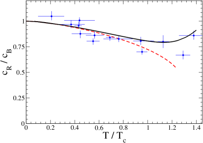
Figure 1: Sound velocity $c_{R}$ in units of $c_{B}=\sqrt{g_{2D}n/m}$ as a function of the scaled temperature $T/T_{c}$ for $\tilde{g}_{2D}\simeq 0.16$. The solid black line represents our prediction based on Eqs. (14) and (15) while the blue dots are the experimental data of Ref. dalibard2017-ictp . The red dashed line is obtained by using Eq. (14) with $c_{I}=0$. On the basis of universal relations prokofev2002 , for $\tilde{g}_{2D}$ the Berezinskii-Kosterlitz-Thouless critical temperature is $T_{c}=0.13\;T_{B}$.

Sound velocity for the 2D Bose gas. In order to describe the behaviour of the quasi-2D uniform Bose gas below or just above the critical temperature, we choose the Bose-Einstein distribution function

$$f_{0}(\mathbf{p})=\frac{1}{L^{2}}\frac{1}{e^{\beta({p^{2}\over 2m}+g_{2D}n-\mu)}-1}\,$$ (11)

as the thermal equilibrium distribution of 2D weakly-interacting bosonic atoms with uniform 2D number density $n=N/L^{2}$, where $\beta\equiv(k_{B}T)^{-1}$, $k_{B}$ is the Boltzmann constant and $T$ is the absolute temperature. Here $\mu$ is the 2D chemical potential of the interacting system. Clearly the Hartree interaction term $g_{2D}n$ can be formally removed by introducing a shifted chemical potential ${\tilde{\mu}}=\mu-g_{2D}n$.

The equation of state, relating the shifted chemical potential ${\tilde{\mu}}$ to the number density $n=N/L^{2}$, is simply derived from the normalization condition

$$N=\int{d^{2}\mathbf{r}d^{2}\mathbf{p}\over(2\pi\hbar)^{2}}f_{0}(\mathbf{p})\;,$$ (12)

resulting in

$${\tilde{\mu}}=k_{B}T\ \ln{\left(1-e^{-T_{B}/T}\right)}$$ (13)

where $k_{B}T_{B}=2\pi\hbar^{2}n/m$ is the temperature of Bose degeneracy and clearly ${\tilde{\mu}}<0$.

The analytical computation of the dispersion relation can be simplified for temperatures $T\ll T_{B}$ and, at the same time, $c_{R}^{2}\ll k_{B}T/m$. Within this range of parameters one is allowed to write $f_{0}(\mathbf{p})L^{2}\simeq k_{B}T/(p^{2}/(2m)-{\tilde{\mu}})$ from which $L^{2}{\tilde{f}}_{0}(p_{x})=k_{B}T/(\hbar\sqrt{(p_{x}^{2}/m)-2{\tilde{\mu}}})$. Consequently, the coupled Eqs. (9) and (10) for the real and imaginary part of the zero-sound velocity respectively read

$$1+\frac{\tilde{g}_{2D}k_{B}T}{2\pi}\Big{[}\frac{2}{mc_{R}^{2}-2{\tilde{\mu}}}+\frac{\sqrt{mc_{R}^{2}}}{(mc_{R}^{2}-2{\tilde{\mu}})^{3/2}}\ln{\bigg{(}\frac{\sqrt{mc_{R}^{2}-2{\tilde{\mu}}}-\sqrt{mc_{R}^{2}}}{\sqrt{mc_{R}^{2}-2{\tilde{\mu}}}+\sqrt{mc_{R}^{2}}}\bigg{)}}\Big{]}+\tilde{g}_{2D}k_{B}Tc_{I}\frac{mc_{R}^{2}+{\tilde{\mu}}}{\sqrt{m}(mc_{R}^{2}-2{\tilde{\mu}})^{5/2}}=0\;,$$ (14)

$$c_{I}=-\frac{\frac{c_{R}}{\sqrt{m}(mc_{R}^{2}-2{\tilde{\mu}})^{3/2}}}{\frac{6\,c_{R}}{(mc_{R}^{2}-2{\tilde{\mu}})^{2}}+\frac{2(mc_{R}^{2}+{\tilde{\mu}})}{\sqrt{m}(mc_{R}^{2}-2{\tilde{\mu}})^{5/2}}\log\Big{(}\frac{\sqrt{mc_{R}^{2}-2{\tilde{\mu}}}-\sqrt{mc_{R}^{2}}}{\sqrt{mc_{R}^{2}-2{\tilde{\mu}}}+\sqrt{mc_{R}^{2}}}\Big{)}}\;.$$ (15)

By inserting Eq. (15) in Eq. (14) we get an equation for $c_{R}$. This equation can be easily solved numerically and, taking into account Eq. (13), one finds the real part $c_{R}$ of the zero-sound velocity as a function of temperature $T$ and adimensional interaction strength ${\tilde{g}}_{2D}$.

In Fig. 1 we compare the solution of Eq. (14) with the experimental data reported in Ref. dalibard2017-ictp . The agreement between our results and the experimental points is excellent in the low-temperature regime and still good close to the superfluid threshold given by the Berezinskii-Kosterlitz-Thouless critical temperature $T_{c}$. The velocity $c_{R}$ does not display any discontinuity at the critical temperature $T_{c}$. This feature marks a crucial difference with respect to first-sound and second-sound velocities calculated within the superfluid Landau-Khalatnikov model, which intrinsically relies upon a collisional dynamics of the normal component ozawa2014 ; stringari-book . Despite the similar behaviour exhibited far below $T_{c}$ by the second-sound velocity $c_{2}$ ota2017 and our collisionless velocity $c_{R}$, the former is related to the superfluid density and consequently it jumps to zero at $T_{c}$ ota2017 .

The dashed line of Fig. 1 is obtained by using Eq. (14) with $c_{I}=0$. Comparing the dashed line with the solid line, which is instead derived solving the coupled Eqs. (14) and (15), one clearly sees the increasingly relevant role played by the imaginary part $c_{I}$ (the so-called Landau damping) above $T_{c}$.

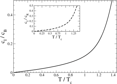
Figure 2: Main panel: Imaginary part $c_{I}$ of the sound velocity in units of $c_{B}=\sqrt{g_{2D}n/m}$ as a function of the scaled temperature $T/T_{c}$ for $\tilde{g}_{2D}\simeq 0.16$. The solid black line is obtained from Eq. (15) where $c_{R}$ has derived by solving Eq. (14). Inset: Ratio between the imaginary and the real part of $c$ as a function of the temperature.

In Fig. 2 we report the absolute value of $c_{I}$ as predicted by Eq. (15), where $c_{R}$ is simply the solution of Eq. (14). We remark that Eq. (9) and (10) are derived by assuming a weakly-damped perturbation, i.e. $c_{I}\ll c_{R}$. ¿From Fig. 2 it appears clear that our approximation scheme is surely reliable for low temperatures, where Landau damping plays a negligible role, but also in the proximity of the transition temperature $T_{c}$. Quite remarkably, the rapid growth of $c_{I}/c_{R}$ with the temperature $T$ above $T_{c}$ is in agreement with the large damping of sound oscillations found in Ref. dalibard2017-ictp . A large value of $c_{I}/c_{R}$ also signals the breaking of our theoretical scheme, also if the theoretical results reproduce the experimental data.

Conclusions. We have analyzed the sound propagation in collisionless bosonic gases assuming a 2D configuration. By solving the linearized 2D Landau-Vlasov equation in the degenerate regime, where bosonic statistical effects play a relevant role, we have derived an integral equation for the speed of sound as a function of temperature and interaction strength. From this integral equation we have obtained two coupled algebraic equations for the real and imaginary part of the sound velocity. We have then compared our theoretical results with experimental data of a recent experiment dalibard2017-pra ; dalibard2017-ictp , where the ⁸⁷Rb atoms of the bosonic cloud are expected to be in the collisionless regime. This expectation is fully confirmed: the agreement betweeen our theory and the experiment is very encouraging. Our theoretical analysis strongly suggests that the density perturbation used in the experiment of Ref. dalibard2017-ictp has excited the ”bosonic zero sound”, i.e. the sound of a collisionless bosonic fluid. For a superfluid system, a density perturbation can be used to excite the second sound only if the system is weakly interacting and collisional ota2017 . By increasing the interaction strength $g_{2D}$ the 2D bosonic system enters in the collisional regime where the Landau-Vlasov equation (2) loses its validity. The collisional regime is in fact correctly described by the two-fluid model of Landau-Khalatnikov which reduces to the usual hydrodynamics above the critical temperature $T_{c}$.

During the final stage of this work, a theoretical preprint on the same topic appeared ota2018 . The conclusions of Ref. ota2018 , based on stochastic Gross-Pitaevskii equation and dynamic response function, are similar to ours.

Acknowledgments. The authors thank Franco Dalfovo for useful discussions. LS acknowledges for partial support the FFABR grant of Italian Ministry of Education, University and Research.

References

- (1) T. R. Kirkpatrick and J. R. Dorfman, Phys. Rev. A 28, 2576(R) (1983).
- (2) T. R. Kirkpatrick and J. R. Dorfman, J. Low Temp. Phys. 58, 301-332 (1985).
- (3) E. Zaremba, A. Griffin and T. Nikuni, Phys. Rev. A 57, 4695 (1998).
- (4) T. Nikuni, E. Zaremba, and A. Griffin, Phys. Rev. Lett. 83, 10 (1999).
- (5) E. Zaremba, T. Nikuni, and A. Griffin, J. Low Temp. Phys. 116, 277-345 (1999).
- (6) A. Griffin, T. Nikuni, and E. Zaremba, Bose-Condensed Gases at Finite Temperatures (Cambridge University Press, New York, 2009).
- (7) A. Vlasov, J. Phys. USSR 9, 25 (1945).
- (8) L. D. Landau, J. Phys. USSR 10, 25 (1946)
- (9) L. D. Landau and E. M. Lifshitz, Course of Theoretical Physics 10: Physical Kinetics (Pergamon International Library, Exeter, 1981).
- (10) L. Kadanoff and G. Baym, Quantum Statistical Mechanics: Green’s Function Methods in Equilibrium and Nonequilibrium Problems (W.A. Benjamin, New York, 1962).
- (11) N. D. Mermin and H. Wagner, Phys. Rev. Lett. 17, 133 (1966).
- (12) P.C. Hohenberg, Phys. Rev. 158, 383 (1967).
- (13) V. L. Berezinskii, Sov. Phys. JETP 34, 610 (1972).
- (14) J. M. Kosterlitz and D. J. Thouless, J. Phys. C: Solid State Phys. 6, 1181 (1973).
- (15) V. P. Singh, C. Weitenberg, J. Dalibard, and L. Mathey, Phys. Rev. A 95, 043631 (2017).
- (16) J.L. Ville, R. Saint-Jalm, E. Le Cerf, M. Aidelsburger, S. Nascimbéne, J. Dalibard, and J. Beugnon, arXiv:1804.04037 (2018).
- (17) M. Ota and S. Stringari, Phys. Rev. A 97, 033604 (2018).
- (18) N. Prokof’ev, O. Ruebenacker and B. Svistunov, Phys. Rev. Lett. 87, 270402 (2001).
- (19) N. Prokof’ev, O. Ruebenacker, and B. Svistunov, Phys. Rev. A 66, 043608 (2002).
- (20) M. Ota, F. Larcher, F. Dalfovo, L. Pitaevskii, N.P. Proukakis, and S. Stringari, arXiv:1804.04032 (2018).
- (21) F. Baldovin, A. Cappellaro, E. Orlandini, and L. Salasnich, J. Stat. Mech. 063303 (2016).
- (22) T. Ozawa and S. Stringari, Phys. Rev. Lett. 112, 025302 (2014).
- (23) L. P. Pitaevskii and S. Stringari, Bose-Einstein Condensation and Superfluidity (Oxford University Press, Oxford, 2016).