Kelvin knots in superconducting state

The failed “vortex-atoms” theory of matter by Kelvin and Tait Thomson (1867); Tait (1898) had a profound impact on mathematics and physics. Building on the understanding of vorticity by Helmholtz, and observing stability of smoke rings, they hypothesised that elementary particles (at that time atoms) are indestructible knotted vortices in luminiferous aether: the hypothetical ideal fluid filling the universe. The vortex-atoms theory identified chemical elements as topologically different vortex knots, and matter was interpreted as bound states of these knotted vortices. This work initiated the field of knot theory in mathematics. It also influenced modern physics, where a close although incomplete analogy exists with the theory of superfluidity, which started with Onsager’s and Feynman’s introduction of quantum vortices Onsager (1949); Feynman (1955). Indeed many macroscopic properties of superconductors and superfluids are indeed determined by vortex lines forming different “aggregate states”, such as vortex crystals and liquids. While crucial importance of knots was understood for many physical systems in the recent years, there is no known physical realization of the central element of Kelvin theory: the stable particle-like vortex knot. Indeed, vortex loops and knots in superfluids and ordinary superconductors form as dynamical excitations and are unstable by Derrick theorem Derrick (1964). This instability in fact dictates many of the universal macroscopic properties of superfluids. Here we show that there are superconducting states with principally different properties of the vorticity: where vortex knots are intrinsically stable. We demonstrate that such features should be realised near certain critical points, where the hydro-magneto-statics of superconducting states yields stables vortex knots which behave similar to those envisaged in Kelvin and Tait’s theory of vortex-atoms in luminiferous aether.

Kelvin’s theory was falsified, when Michelson and Morley’s experiment ruled out the existence of aether. Yet the principle to associate vortices in some underlying field with “elementary particles” re-emerged in two important concepts in modern condensed matter physics: the particle-vortex duality and the interpretation of collective vortex states as “vortex matter”, most notably in superfluidity and superconductivity. These analogies follow developments of three paradigm-shifting concepts introduced in Onsager’s work on superfluids Onsager (1949). First concept was the observation that superfluid velocity circulation is quantized, hence vortices carry a quantized topological charge. Second observation was that rotation of a superfluid results in the formation of a lattice or a liquid of quantum vortices, i.e. the vortex matter realisation of crystals and liquids. The third crucial concept is that vortex matter controls many of the key responses of superfluids. For example, the superfluid to normal state phase transition is a thermal generation and proliferation of vortex loops and knots Onsager (1949). Subsequently this theory was put on firm theoretical grounds by Feynman Feynman (1955). Superconducting phase transition was demonstrated to be driven likewise by proliferation of vortex loops Dasgupta and Halperin (1981). A remarkable analogy with Kelvin’s theory resides in the Berezinskii, Kosterlitz and Thouless theory of two-dimensional superfluids, where vortices with opposite circulations are mapped onto particles and antiparticles. In three dimensions the thermal and quench responses, and turbulent states are collective states of vortex loops and knots. However, the crucial difference with the Kelvin’s theory is that vortex loops and knots are intrinsically unstable, as follows from Derrick’s theorem Derrick (1964). This implies that an excited system forms vortex loops and knots which, however, tend to collapse as the kinetic energy of the superflow always decreases for a smaller loops or knots.

Research on models supporting stable knotted solitons has been of great interest in mathematics and physics after stability of these objects was found in the so-called Skyrme-Faddeev model Faddeev (1975); Gladikowski and Hellmund (1997); Faddeev and Niemi (1997) (for a review, see Radu and Volkov (2008)). It was further observed that there exist a formal relation between Skyrme-Faddeev’s model and ostensibly unrelated, Ginzburg-Landau theories for multicomponent superconductors Babaev et al. (2002); Babaev (2002). Namely, two-component Ginzburg-Landau models can be mapped onto a Skyrme-Faddeev model coupled to an additional massive vector field. This observation motivated the conjecture that multicomponent superconductors may support stable knots. Detailed numerical studies however did not found stability Jäykkä et al. (2008). The reasons for the instability were subsequently discussed both using physical estimates Babaev (2009), and formal mathematical approach Jäykkä and Speight (2011). Despite different analytical arguments in favour of the (meta)stability Babaev (2009); Gorsky et al. (2013), and findings of the stability of knots in mathematical generalisations of Skyrme-Faddeev model coupled to gauge fields Ward (2002); Jäykkä and Speight (2011), the prevalent opinion today is that knotted vortices are unstable in theories of superconductivity as in superfluids.

We demonstrate in this paper, that stable vortex knots exist in two-component superconducting states in a certain parameter range. Many of the superconducting states of interest today have multiple components, for various reasons: e.g. spin-triplet pairing, or nematic states (for recent examples see e.g. Wang et al. (2016); Wang and Fu (2017)), or coexistence of superconductivity of electrons and nucleons Sjöberg (1976); Babaev et al. (2004); Babaev and Ashcroft (2007); Jones (2006). A generic feature of multicomponent superconductors and superfluids is the existence intercomponent current-current interaction, also known as the Andreev-Bashkin effect Andreev and Bashkin (1975); Svistunov et al. (2015). Namely, in superfluid mixtures of two components (labelled “1” and “2”), because of the intercomponent interaction between particles, the current of a given component ${\bm{j}}_{1,2}$ generically depends on the superfluid velocities ${\bm{v}}_{1,2}$ of both, as follows:

$${\bm{j}}_{1}=\rho_{11}{\bm{v}}_{1}+\rho_{12}{\bm{v}}_{2}\,,\leavevmode\nobreak\ \leavevmode\nobreak\ \leavevmode\nobreak\ \text{and}\leavevmode\nobreak\ \leavevmode\nobreak\ \leavevmode\nobreak\ {\bm{j}}_{2}=\rho_{22}{\bm{v}}_{2}+\rho_{21}{\bm{v}}_{1}\,.$$ (1)

There, the coefficients $\rho_{12}$ and $\rho_{21}$ determine the fraction of the density of one of the superfluid component carried by the superfluid velocity of the other: i.e. the intercomponent drag. The drag coefficients $\rho_{12}$ and $\rho_{21}$ can be very large, for example, in spin-triplet superconductors and superfluids Leggett (1975), Fermi-liquids mixtures Sjöberg (1976) or strongly correlated systems Kuklov and Svistunov (2003); Sellin and Babaev (2018).

Two-component superconductors are described by a doublet $\Psi=(\psi_{1},\psi_{2})^{\mathrm{T}}$, of complex fields $\psi_{a}=|\psi_{a}|\text{e}^{i\varphi_{a}}$ (with $a=1,2$), whose squared moduli $|\psi_{a}|^{2}$ represent the density of individual superconducting components. Each of the components is coupled, via the gauge derivative ${\bm{D}}={\bm{\nabla}}+ig{\bm{A}}$, to the vector potential ${\bm{A}}$ of the magnetic field ${\bm{B}}={\bm{\nabla}}\times{\bm{A}}$. Such a system is described by the Ginzburg-Landau free energy $E=\int\mathcal{E}d{\bf r}$, whose density reads as:

$$\mathcal{E} =\frac{{\bm{B}}^{2}}{2}+\sum_{a=1,2}\frac{\gamma_{a}}{2}|{\bm{D}}\psi_{a}|^{2}+\sum_{a,b=1,2}\frac{\mu_{ab}}{2}{\bm{J}}_{a}\cdot{\bm{J}}_{b}$$ (2a)

$$\leavevmode\nobreak\ \leavevmode\nobreak\ \leavevmode\nobreak\ \leavevmode\nobreak\ \leavevmode\nobreak\ \leavevmode\nobreak\ +{\nu}\left(\Psi^{\dagger}\Psi-1\right)^{2}+V[\Psi,\Psi^{\dagger}]\,.$$ (2b)

$$\text{where}\leavevmode\nobreak\ \leavevmode\nobreak\ {\bm{J}}_{a}=\mathrm{Im}(\psi_{a}^{*}{\bm{D}}\psi_{a})=|\psi_{a}|^{2}({\bm{\nabla}}\varphi_{a}+g{\bm{A}})\,.$$

The terms $\mu_{12}=\mu_{21}$ of the current coupling matrix $\hat{\mu}$, describe the intercomponent drag Andreev and Bashkin (1975); Leggett (1975); Sjöberg (1976); Kuklov and Svistunov (2003); Sellin and Babaev (2018). The total current, is the sum of the supercurrents in individual components, which have a similar structure as in (1). The first term in (2b) is responsible for the condensation of superconducting electrons such that, in the ground state, $\Psi^{\dagger}\Psi\neq 0$. Many two-component superconducting states spontaneously break $\mathrm{U}(1)\!\times\!\mathrm{U}(1)$, $\mathrm{U}(1)\!\times\!\mathbb{Z}_{2}$ or $\mathrm{U}(1)$ symmetries (see e.g. Wang et al. (2016); Wang and Fu (2017); Babaev et al. (2004); Babaev and Ashcroft (2007); Jones (2006)). The corresponding symmetry breaking potential terms are collected in $V[\Psi,\Psi^{\dagger}]$. For strongly type-II superconductors a good approximation is the constant-density (London limit), which is equivalent to $\nu\to\infty$ in (2b). The results of this paper were verified to hold for a wide variety of the symmetry-breaking potential terms, whose detailed structure is described in the Methods section.

In two-component superconductors, the simplest vortices feature a $2\pi$ phase winding only in one of the components, e.g. when on a close contour surrounding the vortex core $\oint{\bm{\nabla}}\varphi_{1}\!\cdot\!d{\bm{\ell}}=2\pi$, while $\oint{\bm{\nabla}}\varphi_{2}\!\cdot\!d{\bm{\ell}}=0$. These are called fractional vortices (for details, see e.g. Svistunov et al. (2015)). Topologically nontrivial knotted vortex loops consist of linked or knotted loops of fractional vortices in each component. Like in Kelvin’s theory, there are infinitely many ways to knot and link such objects. Topological considerations imply that knotted vortices are characterized by an integer topological index ${\cal Q}$ (see e.g. discussions in Refs. Faddeev (1975); Faddeev and Niemi (1997); Babaev et al. (2002); Babaev (2002); Jäykkä et al. (2008); Radu and Volkov (2008); Babaev (2009)). This index, which is conserved when fractional vortices in different components cannot cross each other, is defined as (see details in Methods):

$${\cal Q}=-\frac{1}{12\pi^{2}}\int_{\mathbb{R}^{3}}\varepsilon_{ijk}\varepsilon_{abcd}\,\zeta_{a}\frac{\partial\zeta_{b}}{\partial r_{i}}\frac{\partial\zeta_{c}}{\partial r_{j}}\frac{\partial\zeta_{d}}{\partial r_{k}}d{\bf r}\,,$$ (3)

where ${\bm{\zeta}}=\left(\mathrm{Re}\,\psi_{1},\mathrm{Im}\,\psi_{1},\mathrm{Re}\,\psi_{2},\mathrm{Im}\,\psi_{2}\right)/\sqrt{\Psi^{\dagger}\Psi}$, and $\varepsilon$ is the Levi-Civita symbol. The index ${\cal Q}$ is always an integer, unless $\Psi$ has zeros. The situation $\Psi=0$ can appear if cores of fractional vortices overlap. Transient vortex states characterised by such topological index are natural for two-component superfluids and were experimentally observed Lee et al. (2018). In superfluids, however such vortex knots represent non-stationary object: the vortex knots are unstable against shrinkage and the topological index vanishes when the loops shrink.

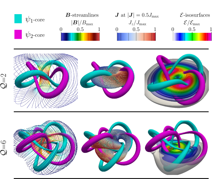
Figure 1: Detailed structure of two stable vortex knots with different morphology. Cyan and magenta tubes denote the positions of the cores of the (fractional) vortices defined as the lines where the densities of a given component, $|\psi_{1}|^{2}$ or $|\psi_{2}|^{2}$, vanish. The tubes here are the density-isosurfaces such that $|\psi_{1,2}|^{2}=2.5\times 10^{-2}$. The panels on the first column show, in addition to the vortex cores, a selection of magnetic field streamlines which circulate within the knot (colored according to the magnitude of $|{\bm{B}}|$), showing chiral structure of the magnetic field. The second column displays the total current structure ${\bm{J}}$ on a selected isosurface where $|{\bm{J}}|/J_{\mathrm{max}}=0.5$. This also shows their chiral structure (the coloring denotes the values of the component $J_{z}$). The last panels show isosurfaces of the energy densities of the vortex knots solutions.

In order to investigate the existence of stable knotted vortices, in two-component superconductors, we performed numerical minimisation of the free energy functional (2), starting from various initial states of knotted and linked vortex loops. The numerical computations are related, in a way, to the relaxation processes of vortex tangles formed due thermal fluctuations or quench. Such three dimensional optimisation problem is a highly computationally demanding task, which we addressed with a code designed for GPUs (see Methods for details). Upon finding stable knotted solutions for various parameters of the model (2), a detailed investigation of solutions for various values of topological index ${\cal Q}$ was performed in the London limit where $\Psi^{\dagger}\Psi=1$ (see Methods for details). We confirm that typically for superconducting models, vortex knots are unstable. This agrees with the phenomenology of common superconducting materials, where, just like in superfluids, the vortex loops minimize their energy by shrinking. However we find that the properties of knotted vorticity become principally different, when the Andreev-Bashkin couplings $\hat{\mu}$ are substantially larger than usual gradient couplings $\gamma_{a}$. Such a disparity between coefficients occurs near two kinds critical points. First is the phase transition to paired phases caused by strong correlations Kuklov and Svistunov (2003); Svistunov et al. (2015); Sellin and Babaev (2018). There the ratio of the stiffnesses of counter- and co-flows of the two components vanishes: which implies that the superconductor acquires arbitrarily strong Andreev-Bashkin coupling by approaching close enough that critical point Sellin and Babaev (2018). Second example is the phase transition to Fulde-Ferrel-Larkin-Ovchinnikov, where the coefficients $\gamma_{a}$ change signs (see e.g. Buzdin and Kachkachi (1997)), while the Andreev-Bashkin interaction remains non-zero. Hence, even systems with relatively weak Andreev-Bashkin interactions $\mu_{ab}$ fullfill the above requirements of the disparity of the coefficients, sufficiently close to Fulde-Ferrel-Larkin-Ovchinnikov phase transition. We find that in such regimes, the energy minimization from entangled vorticity relaxes to stable vortex knots.

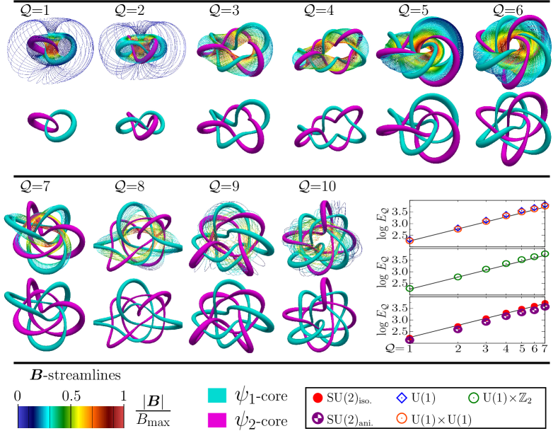
Figure 2: Each panel shows stable knots with increasing topological index ${\cal Q}$=1-10. They consist of two pictures; the lower image displays core structure where, as in Fig. 1, cyan and magenta tubes denote the positions of the core of the (fractional) vortices in each components. The upper image shows in addition to the vortex cores, a selection of magnetic field streamlines circulating within the knot. Note that when increasing the topological index, the structure of magnetic field streamlines becomes increasingly more complex. The last panel shows the dependence of the vortex knots energy $E_{\cal Q}$, as a function the topological index ${\cal Q}$. The curves labelled $\mathrm{SU}(2)_{\mathrm{iso.}}$, $\mathrm{U}(1)\!\times\!\mathbb{Z}_{2}$ , $\mathrm{U}(1)\!\times\!\mathrm{U}(1)$ and $\mathrm{U}(1)$ correspond to knotted solutions in different models with various symmetry-breaking potentials, while the case $\mathrm{SU}(2)_{\mathrm{ani.}}$ corresponds to a symmetry-breaking gradient terms.

The detailed structure for two obtained stable vortex knots is displayed on Fig. 1, for a $\mathrm{U}(1)\!\times\!\mathrm{U}(1)$ superconductor where the parameters $\gamma_{a}=0.02$ and $\mu_{ab}=1$, correspond to a system in the vicinity of the above mentioned phase transitions. Both topologically different solutions consist of linked and knotted loops of fractional vortices, which are visualized by the tubes corresponding to constant-density-isosurfaces around their cores. The energy density of knotted solutions is localized near the knot center, thus emphasizing that these objects are particle-like topological solitons (i.e. localised lumps of energy). The mechanism responsible for the stability of the solutions follows from the nontrivial scaling of magnetic field energy, produced by knotted currents. During the energy minimisation process that starts from a large vortex tangle, the solution first shrinks in order to minimise the kinetic energy of supercurrents. This energy gain is eventually counterbalanced by the raise of magnetic field energy due to the knotted current configuration. By contrast a topologically trivial vortex loop that does not feature helical or knotted currents (such as a loop of a single fractional vortex) trivially shrinks to zero size.

Akin, to the picture envisaged in Kelvin’s theory, the superconducting states here support infinitely many stable solutions corresponding to topologically different ways to tie vortex knots. Figure 2 displays ten stable knotted vortex loops, with smallest topological indices ${\cal Q}=$1-10, in the case of a $\mathrm{U}(1)\!\times\!\mathrm{U}(1)$ superconductor. Animations showing the structure of knotted vortices, and their formation can be found in Supplementary Material. We obtained similar stable solutions for two-component models that break $\mathrm{SU}(2)$, $\mathrm{U}(1)\!\times\!\mathbb{Z}_{2}$ and $\mathrm{U}(1)$ symmetries. The last panel of Fig. 2 shows that the energy of knotted vortices scales with the topological charge as $E_{\cal Q}\propto|{\cal Q}|^{3/4}$. Remarkably the power law is similar to the Vakulenko-Kapitansky law which was derived for the solutions of the Skyrme-Faddeev model. Thus when increasing the topological index, knotted vortices minimize their energy by forming complex bound states of knotted and linked fractional vortices. This is again similar to the picture of matter formation envisaged in Kelvin’s atom theory. The solutions with ${\cal Q}$=1-4 consist of two linked fractional vortex loops twisted around each other different number of times. For ${\cal Q}$=5 the solution instead is a bound state of two pairs of linked fractional vortex loops. The ${\cal Q}$=6 knot consists of two linked trefoils knots. For higher topological indices ${\cal Q}$=7-10, we find that topological structures of the vorticity in different components are inequivalent, the solutions thus forming “isomers”. For example the ${\cal Q}$=7 knot features a fractional vortex in one component forming a trefoil knot, linked with two twisted fractional vortex loops of the other component. For each such isomer solution there is an energetically equivalent solution where the linked vorticity structure is interchanged between the components.

In conclusion, the vortex-atom theory of Kelvin identified chemical elements with knotted vortex loop in luminiferous aether. Remarkably, this theory has profound similarities, but also some important differences with the physics of superconductivity, developed a century later. In particular, the Meissner effect dictates that superconductors can carry magnetic fields and current only in a thin layer near their surface, unless they form quantum vortices. An external magnetic field create vortex lines that terminate on superconductor’s surface. The field-induced vortices form different collective states: lattices, liquids and glasses, all featuring distinct transport properties. To create a current in the bulk of a superconductor, in the absence of an external field, it is required to form a closed vortex loop. Closed loops form dynamically: e.g. due to quenches or thermal fluctuations. The crucial difference with Kelvin’s theory is that in ordinary superconductors vortex loops are not energetically stable. This intrinsic instability of a vortex loop determines the response of superconductors to an external magnetic field, their post-quench relaxation, and their critical properties. We demonstrated that under certain conditions the properties of vortex excitations in a superconductor change radically and knotted vortex loops become stable, akin envisaged in Kelvin theory. We find that this occurs in multicomponent superconductors, at least near certain critical points, for example in the vicinity of Fulde-Ferrel-Larkin-Ovchinnikov states. The energy associated with knotted vorticity starts increasing if vortex knots shrink beyond certain size. Moreover the knots form complicated bound states which is strikingly similar to the matter formation envisaged in Kelvin theory. This stability property of vorticity implies radically different hydro-magnetostatics, compared to ordinary superconductors. This opens-up further questions on the macroscopic properties of these states.

Online Content Methods, along with any additional Extended Data display items and Source Data, are available in the online version of the paper; references unique to these sections appear only in the online paper.

Supplementary Information is available in the online version of the paper.

Acknowledgements We acknowledge fruitful discussions with Johan Carlström, Juha Jäykkä, during various stages of this work. The work was supported by the Swedish Research Council Grants No. 642-2013-7837, No. VR2016-06122 and Göran Gustafsson Foundation for Research in Natural Sciences and Medicine. The computations were performed on resources provided by the Swedish National Infrastructure for Computing (SNIC) at National Supercomputer Center at Linköping, Sweden.

Author Contributions F. N. R. performed finite-difference computations. J. G. performed finite-element computations. All authors contributed to writing the paper.

Methods

Calculation of topological index of vortex knots. Different vortex knots are characterised by an integer index/invariant ${\cal Q}$, associated with the topological properties of the maps $\mathbb{S}^{3}\to\mathbb{S}^{3}_{\Psi}$. To calculate that invariant, the superconducting order parameter field $\Psi$ is cast into a 4-dimensional vector ${\bm{\zeta}}=\left(\mathrm{Re}\,\psi_{1},\mathrm{Im}\,\psi_{1},\mathrm{Re}\,\psi_{2},\mathrm{Im}\,\psi_{2}\right)/\sqrt{\Psi^{\dagger}\Psi}$. Note that for ${\bm{\zeta}}$ to be well defined, there should be no zeros of $\Psi$, i.e. no overlap of the core centers of fractional vortices in both components. If cores of fractional vortices in different components can cross each other, it generates a point where $\Psi^{\dagger}\Psi=0$ and the topological index ${\cal Q}$ is not necessarily an invariant. Namely, it can discretely change from different integer values, when fractional vortices in different components cross each other. The non-crossing requirement is always satisfied in the constant total density limit, i.e. the London limit ($\Psi^{\dagger}\Psi=\mathrm{const}$). Note that when knots are unstable, the invariant changes when they collapse to a size comparable with the numerical lattice size.

Finiteness of the energy implies that the superconductor should be in the ground state at spatial infinity. It follows that infinity is identified with a single field configuration (up to gauge transformations). Hence, the vector field ${\bm{\zeta}}(\mathbf{r})$ is a map from the one-point compactified space to the target 3-sphere ${\bm{\zeta}}:\mathbb{S}^{3}\,[\cong\mathbb{R}^{3}\cup\{\infty\}]\to\mathbb{S}^{3}_{\Psi}$. Maps between 3-spheres fall into disjoint homopoty classes, the elements of the third homotopy group $\pi_{3}(\mathbb{S}^{3}_{\Psi})$, which is isomorphic to integers: $\pi_{3}(\mathbb{S}^{3}_{\Psi})=\mathbb{Z}$. Thereby, ${\bm{\zeta}}$ is associated with an integer number, the degree of the map ${\bm{\zeta}}$: $\mathrm{deg}\,{\bm{\zeta}}$, which counts how many times the target sphere $\mathbb{S}^{3}_{\Psi}$ is wrapped, while covering the whole $\mathbb{R}^{3}$ space. Field configurations are thus characterized by the topological index ${\cal Q}:=\mathrm{deg}\,{\bm{\zeta}}$ which is calculated using equation (3). As discussed, for example, in Jäykkä et al. (2008); Jäykkä and Palmu (2011), the degree of ${\bm{\zeta}}$, ${\cal Q}$ is equal to the Hopf charge of the combined Hopf map $h\circ{\bm{\zeta}}:\mathbb{S}^{3}\to\mathbb{S}^{2}$. The formula (3) was used to calculate the topological invariant of the numerically obtained stable knotted vortex configurations. It was found numerically to be an integer, with the accuracy of a few percent.

Numerical methods and details of the model. The free energy (2) features a potential term $U=\nu(\Psi^{\dagger}\Psi-1)^{2}$, responsible for the nonzero superconducting ground state $\Psi^{\dagger}\Psi\neq 0$. It is supplemented by additional terms, which explicitly break global $\mathrm{SU}(2)$ symmetry of $U$ down to different subgroups

$$V[\Psi,\Psi^{\dagger}]=\sigma|\psi_{1}|^{2}|\psi_{2}|^{2}+\eta\left(\psi_{1}\psi_{2}^{*}+\psi_{1}^{*}\psi_{2}\right)\,.$$ (4)

The solutions were obtained for the parameters of kinetic term $\gamma_{a}=0.02$ and of the current coupling coefficients $\mu_{ab}=1$ for $a,b=1,2$ (except in the $\mathrm{SU}(2)_{\mathrm{ani.}}$ case described below). The gauge coupling constant, used to parametrize the London penetration depth, was set to $g=1$. In order to demonstrate that the existence of stable knotted vortices does not rely on a specific symmetry of the model, we performed computations for various representative symmetry breaking potentials: $\bm{\mathrm{U}(1)}$: $\sigma=-10^{-4}$, $\eta=-5\cdot 10^{-5}$; $\bm{\mathrm{U}(1)\!\times\!\mathbb{Z}_{2}}$: $\sigma=10^{-4}$, $\eta=0$; $\bm{\mathrm{U}(1)\!\times\!\mathrm{U}(1)}$: $\sigma=-10^{-4}$, $\eta=0$; $\bm{\mathrm{SU}(2),\mathrm{iso.}}$: $\sigma=0$, $\eta=0$; $\bm{\mathrm{SU}(2),\mathrm{ani.}}$: for this particular case the ground state is invariant under $\mathrm{SU}(2)$ rotations, but the current-current coupling coefficients were chosen to break that symmetry: $\mu_{11}=\mu_{22}=0.97$ and $\mu_{12}=\mu_{21}=1$. The symmetry-breaking parameters were chosen to be small to avoid important changes in the intrinsic length scales, and thus to prevent substantial changes of the solution size relative to the numerical lattice spacing. That allowed a quantitatively accurate comparison of knotted solutions for different symmetry-breaking potentials.

In our preliminary simulations, we considered various values of the coefficient $\nu$. When stable vortex knots exits they have no zeroes of total density. The stability properties of the solutions were typically better by increasing $\nu$ (i.e. stronger type-II regimes). However, such a regime significantly inhibits the convergence of conventional methods of minimization. This phenomenon is directly related with a well-known disadvantage of penalty function method. Thus after finding stable solutions, with different indices ${\cal Q}$, in several simulations with variable total density, we reduced the size of the parameter space by focusing on the London limit where $\Psi^{\dagger}\Psi=1$ in order to systematically investigate the solutions with topological index ranging from ${\cal Q}=1$ to ${\cal Q}=10$.

For computationally efficient investigation of the London limit we used the “Atlas” method, which is based on an efficient navigation in the coordinate charts for the order parameter manifold, which here is an $\mathbb{S}^{3}_{\Psi}$. (for details of the method see Supplementary Material in Ref. Rybakov et al. (2015)). Its advantage is that it automatically satisfies the constraint, being in conjunction with conventional unconstrained minimisation techniques.

The fields were discretised using a second-order accuracy finite-difference scheme, on an homogeneous cuboidal mesh with lattice spacing $0.5$. The grid used consist on $160^{3}$ nodes for the solutions with $Q\leq 7$ and $224^{3}$ nodes, for higher topological charges. In order to ensure that the solutions are not artefacts of a finite simulation domain, we considered both ‘fixed’ and ‘free’ boundary conditions. The energy was minimised using a nonlinear conjugate gradient (NCG) method with Polak-Ribière-Polyak formula Polak and Ribière (1969); Polyak (1969). We used a branched approach to standard NCG by separating all degrees of freedom into two sets. One associated with gauge degrees of freedom $\mathbf{A}$, and another with the superconducting degrees of freedom $\psi_{a}$. Accordingly, the conventional linear search routine for NCG method was replaced by two-dimensional search. By separating the numerical degrees of freedom according to their physical nature, this approach significantly accelerates the convergence speed of the algorithm. The termination criterion for convergence was chosen according to Gill et al. (1981) with a function tolerance $\tau_{F}\!=\!10^{-10}$. The algorithm was parallelized for NVIDIA CUDA-enabled graphics processor units. Calculations were performed on a set of two video cards with microprocessors GP102-350-K1-A1. In order to achieve maximum performance, most computations were realized using single-precision floating-point format (32 bits). To offset the truncation errors from the single-precision arithmetic, we used Kahan summation algorithm Kahan (1965) and a parallel reduction technique suitable for CUDA Luitjens (2014).

In order to cross-validate our results, we performed few simulations beyond the London limit using a different approach based on a finite-element methods, and found consistent results. The fields were discretized within a framework provided by the FreeFem++ library Hecht (2012). The simulations were typically performed on four, two-sockets nodes, with 8-core Intel Xeon E5-2660 processors.

Initial states for energy-minimization calculations. The energy minimization calculations were seeded with a vorticity-generating initial state based on a hedgehog-type texture Skyrme (1961)

$$(\zeta^{\prime}_{1},\zeta^{\prime}_{2},\zeta^{\prime}_{3})=\mathbf{m}\sin(\chi),\quad\zeta^{\prime}_{4}=\cos(\chi)\,,$$ (5)

where the unit vector field $\mathbf{m}$ is defined as

$$m_{1}+im_{2}=\sin(\vartheta)e^{-iQ\phi},\quad m_{3}=\cos(\vartheta),$$

and the shape function

$$\chi=\pi\left(1+(r/r_{0})^{2}e^{(r/r_{0})^{2}}\right)^{-1}\,,$$

where $r$, $\vartheta$, $\phi$ are the spherical coordinates, and $r_{0}$ is a tunable parameter which sets the appropriate scale of the texture. For the initial state to satisfy the appropriate behaviour at $r\rightarrow\infty$, the vector $\mathbf{\zeta^{\prime}}$ has to be rotated: $\mathbf{\zeta}=R\cdot\mathbf{\zeta^{\prime}}$. The generic rotation matrix, and a particular one, $\tilde{R}$, in the case of the potential yielding a $\mathrm{U}(1)\!\times\!\mathbb{Z}_{2}$ symmetry of the ground state, are defined

$$R=\frac{1}{2}\begin{pmatrix}1&1&-1&1\\ -1&1&1&1\\ 1&-1&1&1\\ -1&-1&-1&1\end{pmatrix}\,,\leavevmode\nobreak\ \leavevmode\nobreak\ \tilde{R}=\frac{1}{\sqrt{2}}\begin{pmatrix}0&0&-1&1\\ 0&0&1&1\\ 1&-1&0&0\\ -1&-1&0&0\end{pmatrix}\,.$$ (6)

Thus, at the boundaries of simulation domain the superconducting degrees of freedom assume ${\bm{\zeta}}=(1,1,1,1)/2$, except in the case of the $\mathrm{U}(1)\!\times\!\mathbb{Z}_{2}$ symmetry where ${\bm{\zeta}}=(1,1,0,0)/\sqrt{2}$. The vector potential is initially set to be a pure gauge $\mathbf{A}\!=\!0$.

Such initial state generates linked vorticity for which the topological charge $Q$ is an input parameter. We observed that for regimes with stable knots the total topological charge remains invariant in the process of minimization. To obtain solutions with high topological index ${\cal Q}$, we placed two separated textures along the main diagonal of computational domain with charges ${\cal Q}_{1,2}$ such that ${\cal Q}_{1}+{\cal Q}_{2}={\cal Q}$. For example, to construct a ${\cal Q}$=1 solution, the starting configuration was ${\cal Q}_{1}$=-1, ${\cal Q}_{2}$=2; for ${\cal Q}$=2 we used ${\cal Q}_{1}={\cal Q}_{2}=1$, etc. During the minimization process, the two initially separated textures attracted and eventually merged into a single one. Such an approach starting with two well separated vorticity-seeding initial states, instead of a single one is very efficient because it breaks spatial symmetries, thus minimizing chances of being trapped in long-living unstable or weakly metastable states.

References

- Thomson (1867) William Thomson, “On Vortex Atoms,” Proceedings of the Royal Society of Edinburgh VI, 94–105 (1867), [Reprinted in Phil. Mag. Vol. XXXIV, 1867, pp. 15-24.].
- Tait (1898) P. G. Tait, “On Knots I II, and III,” Scientific Papers (Cambridge University Press) 1, 273–347 (1898).
- Onsager (1949) L. Onsager, “Statistical hydrodynamics,” Il Nuovo Cimento 6, 279–287 (1949).
- Feynman (1955) R.P. Feynman, “Application of Quantum Mechanics to Liquid Helium,” Progress in Low Temperature Physics Volume 1, 17–53 (1955).
- Derrick (1964) G. H. Derrick, “Comments on Nonlinear Wave Equations as Models for Elementary Particles,” Journal of Mathematical Physics 5, 1252–1254 (1964).
- Dasgupta and Halperin (1981) C. Dasgupta and B. I. Halperin, “Phase Transition in a Lattice Model of Superconductivity,” Phys. Rev. Lett. 47, 1556–1560 (1981).
- Faddeev (1975) L. D. Faddeev, “Quantization of Solitons,” in Preprint IAS Print-75-QS70 (Inst. Advanced Study, Princeton, NJ) (1975).
- Gladikowski and Hellmund (1997) Jens Gladikowski and Meik Hellmund, “Static solitons with non-zero Hopf number,” Phys. Rev. D 56, 5194–5199 (1997).
- Faddeev and Niemi (1997) L. D. Faddeev and Antti J. Niemi, “Knots and particles,” Nature 387, 58 (1997).
- Radu and Volkov (2008) Eugen Radu and Mikhail S. Volkov, “Existence of stationary, non-radiating ring solitons in field theory: knots and vortons,” Phys. Rept. 468, 101–151 (2008).
- Babaev et al. (2002) Egor Babaev, L. D. Faddeev, and Antti J. Niemi, “Hidden symmetry and knot solitons in a charged two- condensate Bose system,” Phys. Rev. B 65, 100512 (2002).
- Babaev (2002) Egor Babaev, “Dual Neutral Variables and Knot Solitons in Triplet Superconductors,” Phys. Rev. Lett. 88, 177002 (2002).
- Jäykkä et al. (2008) Juha Jäykkä, Jarmo Hietarinta, and Petri Salo, “Topologically nontrivial configurations associated with Hopf charges investigated in the two-component Ginzburg-Landau model,” Phys. Rev. B 77, 094509 (2008).
- Babaev (2009) Egor Babaev, “Non-Meissner electrodynamics and knotted solitons in two- component superconductors,” Phys. Rev. B 79, 104506 (2009).
- Jäykkä and Speight (2011) J. Jäykkä and J. M. Speight, “Supercurrent coupling destabilizes knot solitons,” Phys. Rev. D 84, 125035 (2011).
- Gorsky et al. (2013) A. Gorsky, M. Shifman, and A. Yung, “Revisiting the Faddeev-Skyrme model and Hopf solitons,” Phys. Rev. D 88, 045026 (2013).
- Ward (2002) R S Ward, “Stabilizing textures with magnetic fields,” Phys. Rev. D 66, 041701 (2002).
- Wang et al. (2016) Yuxuan Wang, Gil Young Cho, Taylor L. Hughes, and Eduardo Fradkin, “Topological superconducting phases from inversion symmetry breaking order in spin-orbit-coupled systems,” Phys. Rev. B 93, 134512 (2016).
- Wang and Fu (2017) Yuxuan Wang and Liang Fu, “Topological Phase Transitions in Multicomponent Superconductors,” Phys. Rev. Lett. 119, 187003 (2017).
- Sjöberg (1976) O. Sjöberg, “On the Landau effective mass in asymmetric nuclear matter,” Nuclear Physics A 265, 511–516 (1976).
- Babaev et al. (2004) E. Babaev, A. Sudbø, and N. W. Ashcroft, “A superconductor to superfluid phase transition in liquid metallic hydrogen,” Nature 431, 666–668 (2004).
- Babaev and Ashcroft (2007) Egor Babaev and N. W. Ashcroft, “Violation of the London law and Onsager-Feynman quantization in multicomponent superconductors,” Nature Physics 3, 530–533 (2007).
- Jones (2006) P. B. Jones, “Type I and two-gap superconductivity in neutron star magnetism,” Monthly Notices of the Royal Astronomical Society 371, 1327–1333 (2006).
- Andreev and Bashkin (1975) A. F. Andreev and E. P. Bashkin, “Three-velocity hydrodynamics of superfluid solutions,” Soviet Journal of Experimental and Theoretical Physics 42, 164 (1975), zh. Eksp. Teor. Fiz. 69, 319-326 (1975).
- Svistunov et al. (2015) B.V. Svistunov, E.S. Babaev, and N.V. Prokof’ev, Superfluid States of Matter (Taylor & Francis, 2015).
- Leggett (1975) Anthony J. Leggett, “A theoretical description of the new phases of liquid 3He,” Rev. Mod. Phys. 47, 331–414 (1975).
- Kuklov and Svistunov (2003) A. B. Kuklov and B. V. Svistunov, “Counterflow Superfluidity of Two-Species Ultracold Atoms in a Commensurate Optical Lattice,” Phys. Rev. Lett. 90, 100401 (2003).
- Sellin and Babaev (2018) Karl Sellin and Egor Babaev, “Superfluid drag in the two-component Bose-Hubbard model,” Phys. Rev. B 97, 094517 (2018).
- Lee et al. (2018) Wonjae Lee, Andrei H. Gheorghe, Konstantin Tiurev, Tuomas Ollikainen, Mikko Möttönen, and David S. Hall, “Synthetic electromagnetic knot in a three-dimensional skyrmion,” Science Advances 4 (2018).
- Buzdin and Kachkachi (1997) A.I. Buzdin and H. Kachkachi, “Generalized Ginzburg-Landau theory for nonuniform FFLO superconductors ,” Physics Letters A 225, 341 – 348 (1997).

References

- Jäykkä and Palmu (2011) Juha Jäykkä and Joonatan Palmu, “Knot solitons in a modified Ginzburg-Landau model,” Phys. Rev. D 83, 105015 (2011).
- Rybakov et al. (2015) Filipp N. Rybakov, Aleksandr B. Borisov, Stefan Blügel, and Nikolai S. Kiselev, “New Type of Stable Particlelike States in Chiral Magnets,” Phys. Rev. Lett. 115, 117201 (2015).
- Polak and Ribière (1969) E. Polak and G. Ribière, “Note sur la convergence de directions conjuguée,” Revue française d’informatique et de recherche opérationnelle. Série rouge 3, 35–43 (1969).
- Polyak (1969) B.T. Polyak, “The conjugate gradient method in extremal problems,” USSR Computational Mathematics and Mathematical Physics 9, 94 – 112 (1969), [ Zh. vy’chisl. Mat. mat. Fiz., 9, 4, 807-821 ( 1969)].
- Gill et al. (1981) P.E. Gill, W. Murray, and M.H. Wright, Practical optimization (Academic Press, 1981).
- Kahan (1965) W. Kahan, “Pracniques: Further Remarks on Reducing Truncation Errors,” Commun. ACM 8, 40 (1965).
- Luitjens (2014) J. Luitjens, Faster Parallel Reductions on Kepler, NVIDIA Documentation (2014).
- Hecht (2012) F. Hecht, “New development in freefem++,” J. Numer. Math. 20, 251–265 (2012).
- Skyrme (1961) T. H. R. Skyrme, “A Nonlinear field theory,” Proc. Roy. Soc. Lond. A260, 127–138 (1961).