Close evaluation of layer potentials in three dimensions

Abstract

We present a simple and effective method for evaluating double- and single-layer potentials for Laplace’s equation in three dimensions close to the boundary. The close evaluation of these layer potentials is challenging because they are nearly singular integrals. The method we propose is based on writing these layer potentials in spherical coordinates where the point at which their kernels are peaked maps to the north pole. An $N$-point Gauss-Legendre quadrature rule is used for integration with respect to the the polar angle rather than the cosine of the polar angle. A $2N$-point periodic trapezoid rule is used to compute the integral with respect to the azimuthal angle which acts as a natural and effective averaging operation in this coordinate system. The numerical method resulting from combining these two quadrature rules in this rotated coordinate system yields results that are consistent with asymptotic behaviors of the double- and single-layer potentials at close evaluation distances. In particular, we show that the error in computing the double-layer potential, after applying a subtraction method, is quadratic with respect to the evaluation distance from the boundary, and the error is linear for the single-layer potential. We improve upon the single-layer potential by introducing an alternate approximation based on a perturbation expansion and obtain an error that is quadratic with respect to the evaluation distance from the boundary.

Keywords: Nearly singular integrals, close evaluation problem, potential theory, boundary integral equations, numerical quadrature.

1 Introduction

The close evaluation problem arises when using boundary integral methods to solve boundary value problems for linear, elliptic partial differential equations. In boundary integral methods, the solution of the boundary value problem is given in terms of double- and single-layer potentials, integrals of a kernel multiplied by a density over the boundary of the domain. The kernel for the single-layer potential is the fundamental solution of the elliptic partial differential equation and the kernel for the double-layer potential is the normal derivative of that fundamental solution. Each of these kernels has an isolated singularity at a known point on the boundary. When evaluating layer potentials at points close to the boundary, the associated kernel is regular, but is sharply peaked. For this reason, we say that layer potentials evaluated close to the boundary are nearly singular integrals.

Nearly singular integrals are more challenging to compute numerically than weakly singular ones, resulting from evaluating layer potentials at points on the boundary. When computing weakly singular integrals, one explicitly addresses the singularity in the kernel. There are several high-order methods available to compute weakly singular integrals (e.g. [6, 11, 19, 17, 10]). For example, they can be computed accurately using high-order product Nyström methods [6, 14] that analytically treat integration over the singular point. These product Nyström methods are often used to solve the boundary integral equations for the density. However, for a nearly singular integral, there is no singularity to address. Nonetheless, without effectively addressing the peaked behavior in a nearly singular integral for an evaluation point fixed close to the boundary, one must increase the number of quadrature points to obtain accuracy commensurate with evaluation points that are far from the boundary.

There are two factors that affect the accuracy of a numerical method for the close evaluation problem: the distance from the boundary and the number of quadrature points. Based on these two factors, one can design a new competitive numerical method (improving the convergence rate with respect to the number of quadrature points), or one can provide corrections to existing ones (improving the convergence rate with respect to the distance for a fixed number of quadrature points). Here, we focus on this second consideration.

The close evaluation problem has been studied extensively for two-dimensional problems. Schwab and Wendland [28] have developed a boundary extraction method based on a Taylor series expansion of the layer potentials. Beale and Lai [8] have developed a method that first regularizes the nearly singular kernel and then adds corrections for both the discretization and the regularization. The result of this approach is a uniform error in space. Helsing and Ojala [22] developed a method that combines a globally compensated quadrature rule and interpolation to achieve very accurate results over all regions of the domain. Barnett [7] has used surrogate local expansions with centers placed near, but not on, the boundary. These results led to the work by Klöckner et al. [25] that introduces Quadrature By Expansion (QBX). QBX uses expansions about accurate evaluation points far away from the boundary to compute accurate evaluations for points close to it. The convergence of QBX has been studied in [15]. Moreover, fast implementations of QBX have since been developed [1, 26, 30], and rigorous error estimates have been derived for the method [2]. Recently, the authors have developed a method that involves matched asymptotic expansions for the kernel of layer potentials [12]. In that method, the asymptotic expansion that captures the peaked behavior of the kernel can be integrated exactly using Fourier series, and the relatively smooth remainder is integrated numerically, resulting in a highly accurate method.

There are fewer results for three-dimensional problems. Beale et al. [9] have extended the regularization method to three-dimensional problems. Additionally, QBX has been used for three-dimensional problems [1, 30]. In principle, the matched asymptotic expansion method developed by the authors for two dimensions can be extended to three-dimensional problems (using spherical harmonics instead). However, we do not pursue that approach because the method we present here is direct and simple to implement. The development of accurate numerical methods in three dimensions can be challenging and there is a need for such methods that are straightforward to implement.

Further, there exist quadrature methods to specifically deal with nearly singular integrals. Johnston and Elliot [24] introduce a hyperbolic sine transformation to cluster quadrature points around the near singularity of the kernel. This clustering of points is dependent on the peakedness of the kernel and location of the singularity. Iri, Moriguti, and Takasawa  [23] have developed a method for nearly singular integrals that takes advantage of the spectral accuracy of the periodic trapezoid rule. This method also results in a clustering of quadrature points around the near singularity of the kernel.

In this paper, we study the close evaluation of double- and single-layer potentials for Laplace’s equation in three dimensions. We compute the double- and single-layer potentials in spherical coordinates where the isolated singular point on the boundary is aligned with the north pole, possibly after a rotation. At close evaluation distances, we show that the leading asymptotic behaviors for the kernels of both the double- and single-layer potentials are azimuthally invariant. It follows that integrating over the azimuth in this spherical coordinate system introduces a natural averaging operation that effectively smooths the nearly singular behavior of the layer potentials. We use these asymptotic results to introduce a simple and effective numerical method for computing the close evaluation of double- and single-layer potentials. Comparisons with other quadrature methods designed for nearly singular integrals show that the proposed method is more accurate.

We precisely define the close evaluation problem for the double and single-layer potentials in Section 2. We present in Section 3 some prior quadrature methods for the close evaluation problem. In Section 4, we derive the asymptotic behavior of the contributions to the double and single-layer potentials made by a small region of the boundary containing the point where the kernels are peaked. By doing so, we find a natural numerical method to evaluate these nearly singular integrals. This numerical method is given in Section 5, and improvements for the single-layer potential are considered in Section 6. Several examples demonstrating the accuracy of this numerical method are presented in Section 7. Section 8 gives our conclusions. The details of the method we use to rotate the integrals in spherical coordinates is given in A.

2 Close evaluation of layer potentials

Consider a simply connected, open set denoted by $D\subset\mathbb{R}^{3}$ with smooth oriented boundary, $B$, and let $\bar{D}=D\cup B$. The function $u\in C^{2}(D)\cap C^{1}(\bar{D})$ satisfying Laplace’s equation, $\Delta u=0$, can be expressed using a representation formula, a combination of double- and single-layer potentials [21]:

$$u(x)=-\frac{1}{4\pi}\int_{B}\frac{n(y)\cdot(x-y)}{|x-y|^{3}}u(y)\,\mathrm{d}\sigma_{y}+\frac{1}{4\pi}\int_{B}\frac{1}{|x-y|}\partial_{n}u(y)\,\mathrm{d}\sigma_{y},\quad x\in D,$$ (2.1)

where $n(y)$ is the outward unit normal at $y\in B$ and $\mathrm{d}\sigma_{y}$ is the surface element.

Throughout this paper, we consider (2.1), which corresponds to the representation formula for interior problems. To consider the representation formula for exterior problems, $n(y)$ can just be replaced by $-n(y)$ in (2.1). The solution of the interior Dirichlet problem for Laplace’s equation is often represented using only the double-layer potential (first term in (2.1)) with $u$ replaced by a general density $\mu$. The solution of the exterior Neumann problem for Laplace’s equation is often represented using only the single-layer potential (second term in (2.1)) with $\partial_{n}u$ replaced by a general density $\rho$. For those problems, the densities $\mu$ and $\rho$ satisfy boundary integral equations which can be solved accurately using Nyström methods [6, 14]. Nonetheless, the close evaluation problem for the double-layer potential for the interior Dirichlet problem and for the single-layer potential for the exterior Neumann problem still remains a subject of active investigation. Here, we choose to study the close evaluation of (2.1) since it includes both the close evaluation of the double- and single-layer potentials.

Assuming that both $u$ and $\partial_{n}u$ on $B$ are known, one can use high-order quadrature rules [14] to evaluate (2.1) with high accuracy. However, this high accuracy is lost for evaluation points that are close to, but off the boundary. To understand why this happens, we write a close evaluation point $x\in D$ as,

$$x=y^{\star}-\varepsilon\ell n^{\star},$$ (2.2)

where $0<\varepsilon\ll 1$ is a small, dimensionless parameter, $y^{\star}\in B$ is the point closest to $x$ on the boundary, $n^{\star}=n(y^{\star})$ is the unit, outward normal from $D$ at $y^{\star}$, and $\ell$ is a characteristic length of $B$ associated with $y^{*}$, such as the radius of mean curvature, as shown in Fig. 1.

Figure 1: Schematic presenting the notation given in (2.2).

By substituting (2.2) into (2.1), and making use of Gauss’ law [21],

$$\frac{1}{4\pi}\int_{B}\frac{n(y)\cdot(x-y)}{|x-y|^{3}}\mathrm{d}\sigma_{y}=\begin{cases}-1&x\in D,\\ -\frac{1}{2}&x\in B,\\ \,\,\,\,0&x\in\mathbb{R}^{3}\backslash\bar{D},\end{cases}$$ (2.3)

we can rewrite the representation formula, (2.1), evaluated at the close evaluation point, (2.2), as

$$u(y^{\star}-\varepsilon\ell n^{\star})=u(y^{\star})-\frac{1}{4\pi}\int_{B}\frac{n(y)\cdot(y^{\star}-y-\varepsilon\ell n^{\star})}{|y^{\star}-y-\varepsilon\ell n^{\star}|^{3}}\left[u(y)-u(y^{\star})\right]\mathrm{d}\sigma_{y}+\frac{1}{4\pi}\int_{B}\frac{1}{|y^{\star}-y-\varepsilon\ell n^{\star}|}\partial_{n}u(y)\,\mathrm{d}\sigma_{y}.$$ (2.4)

We call (2.4) the modified representation formula resulting from applying a subtraction method [14] to the double-layer potential in (2.1).

The close evaluation of (2.4) corresponds to the asymptotic limit, $\varepsilon\to 0^{+}$ and in that case the integrals in (2.4) are nearly singular. Setting $\varepsilon=0$ in (2.4) we find that the kernels become singular at $y=y^{\star}$, but those singularities are integrable. Nearly singular integrals place high demands on any numerical integration method since there are no explicit singularities that can be treated analytically. Consequently, these nearly singular integrals require the development of specialized methods to handle the sharply peaked integrands, which is challenging if the error is to be uniformly bounded over the entire domain.

In our analysis and presentation of a new method, we assume $B$ is an analytic and closed oriented surface that can be parameterized using spherical coordinates, $y=y(s,t)$ with $s\in[0,\pi]$ and $t\in[-\pi,\pi]$, where $s$ denotes the polar angle, and $t$ denotes the azimuthal angle. In these coordinates, we assume we have rotated the domain to set $y^{\star}=y(0,\cdot)$, where $y(0,\cdot)$ denotes the spherical mean, $y(0,\cdot):=\lim\limits_{s\to 0^{+}}\displaystyle\frac{1}{2\pi}\int_{-\pi}^{\pi}y(s,t)\,dt$. In other words, $y^{\star}$ is aligned with the north pole, where we make use of the spherical mean to define all quantities. This notation will be used throughout the paper to denote the spherical mean. Note that one can always apply a rotation so that any chosen $y^{\star}$ maps to $y(0,\cdot)$. The expression of the transformation matrix we use for this rotation can be found in A. Using this parametrization and rotation, we write the integrals in (2.4) as,

$$I(y^{\star})=\frac{1}{4\pi}\int_{-\pi}^{\pi}\int_{0}^{\pi}\tilde{F}(s,t)\,\mathrm{d}s\mathrm{d}t\,,$$ (2.5)

with

$$\tilde{F}(s,t)=-\frac{\tilde{n}(s,t)\cdot(y(0,\cdot)-y(s,t)-\varepsilon\ell n^{\star})}{|y(0,\cdot)-y(s,t)-\varepsilon\ell n^{\star}|^{3}}\tilde{J}(s,t)\left[\tilde{\mu}(s,t)-\tilde{\mu}(0,\cdot)\right]+\frac{1}{|y(0,\cdot)-y(s,t)-\varepsilon\ell n^{\star}|}\tilde{J}(s,t)\tilde{\rho}(s,t)\,,$$ (2.6)

where $\tilde{J}(s,t)=|\partial_{s}y(s,t)\times\partial_{t}y(s,t)|$, $\tilde{n}(s,t)=n(y(s,t))$, $\tilde{\mu}(s,t)=\mu(y(s,t))$, and $\tilde{\rho}(s,t)=\rho(y(s,t))$. Note that $n^{\star}=\tilde{n}(0,\cdot)$. For simplicity, we have replaced $u$ by $\mu$ and $\partial_{n}u$ by $\rho$, and we assume $\mu$ and $\rho$ are known and smooth.

3 Prior quadrature methods developed for the close evaluation problem

In this manuscript, we present a new numerical method for computing (2.4) that is based on an asymptotic analysis as $\varepsilon\to 0^{+}$. As stated in the introduction, quadrature methods have been previously developed to accurately approximate nearly singular integrals. In this section, we give three examples of commonly used existing methods that we will compare to our new method in Section 7.

The three quadrature rules we present here are (1) the product Gauss quadrature rule by Atkinson [3] (PGQ) which uses Gauss-Legendre quadrature abscissas in the polar angle, (2) a hyperbolic sine tranformation presented by Johnston and Elliot in [24] (SINH), and (3) a quadrature formula presented by Iri, Moriguti, and Takasawa in [23] with the implementation as given in Robinson and Doncker [27] (IMT). All three methods are defined on a domain, $(z,t)\in[-1,1]\times[-\pi,\pi]$, and use the common substitution for the polar angle for integrals in spherical coordinates, $z=\cos(s)$ where $s\in[0,\pi]$ [3]. Let $z_{i}\in(-1,1)$ for $i=1,\cdots,N$ denote the $N$-point quadrature rule abscissas with corresponding weights, $w_{i}$ and then $s_{i}=\cos^{-1}(z_{i})$ for the abscissas in the polar angle. For all three methods, we use the periodic trapezoid rule in the azimuthal direction. Let $t_{j}=-\pi+\pi(j-1)/N\in[-\pi,\pi]$ for $j=1,\cdots,2N$ denote the equi-spaced grid points for the periodic trapezoid rule. This results in the numerical method

$$I(y^{\star})\approx I^{N}(y^{\star})=\frac{1}{4N}\sum_{i=1}^{N}\sum_{j=1}^{2N}w_{i}\tilde{F}(s_{i},t_{j})\,,$$ (3.1)

to evaluate (2.5) where $s_{i}$ and $w_{i}$ differ between the three methods.

We present numerical results for the solution of Laplace’s equation using the modified representation formula, (2.4), for close evaluation points interior to a peanut-shaped domain presented in Atkinson [4, 5]. The boundary of this domain is given by,

$$y(\theta,\varphi)=r(\theta)(\sin\theta\cos\varphi,2\sin\theta\sin\varphi,\cos\theta),\quad\theta\in[0,\pi],\quad\varphi\in[-\pi,\pi],$$ (3.2)

where

$$r(\theta)=\sqrt{\cos 2\theta+\sqrt{1.1-\sin^{2}2\theta}}.$$ (3.3)

Recall, for each $y^{\star}$, the boundary and domain is rotated from the $(\theta,\phi)$ coordinate system to the $(s,t)$ coordinate system so that $y^{\star}=y(0,\cdot)$. We present results for all three methods at one $y^{\star}$ with varying $\varepsilon$ ($\ell=1$) values, as shown in Fig. 2A. We consider the exact solution, from Beale et al. [9],

$$u_{\text{ex}}(x_{1},x_{2},x_{3})=e^{x_{3}}(\sin x_{1}+\sin x_{2}),$$ (3.4)

with $(x_{1},x_{2},x_{3})$ denoting an ordered triple in a Cartesian coordinate system. We substitute (3.4) evaluated on the boundary and its normal derivative evaluated on the boundary into (2.4) and compute numerical approximations of this harmonic function using (3.1).

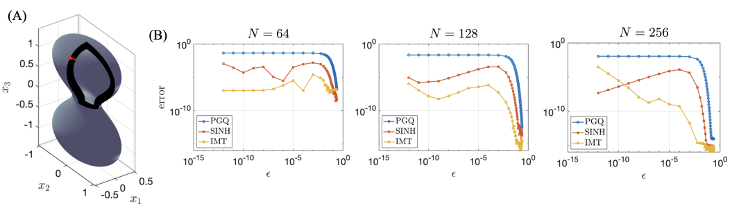
Figure 2: (A) The peanut-shaped domain and the point $y^{\star}=(-0.4349,0,1.1819)$ (red star) with varying $\varepsilon$ values (red line) at which we compute the error in evaluating (2.4) using (3.1) with three different methods. (B) The logarithmic error as a function of $\varepsilon$ for the three quadrature rules used, PGQ, SINH, and IMT, to evaluate (3.1) for three fixed values of $N$.

In Fig. 2B, we present the error with respect to $\varepsilon$ when evaluating (2.4) with the three numerical methods for different fixed $N$ values, $N=64$, $128$, and $256$. The PGQ is a method often used for evaluating double- and single-layer potentials in three dimensions but does not treat the close evaluation problem directly. This is what we observe here as the PGQ has large errors for all values of fixed $N$ as $\varepsilon\to 0^{+}$. The other two quadrature methods, SINH and IMT, are specifically designed for nearly singular integrals and choose abscissas such that more quadrature points are located near the nearly singular point, $s=0$, see Fig. 5. We refer the reader to [23, 24, 27] for details on how these abscissas and corresponding weights are chosen. We point out the implementation of these two methods pose some challenges, including that the IMT quadrature requires the use of a table for the abscissas and weights and the SINH quadrature rule requires using $\varepsilon$ to determine appropriate abscissas and weights. We first observe in Fig. 2 that the SINH and IMT methods do improve the error in the close evaluation problem and the errors are not monotonic in $\varepsilon$. The SINH quadrature for a fixed $N$ that is large, $N=256$, does exhibit some convergence but is at a rate significantly less than $O(\varepsilon)$.

Furthermore, for these methods we do not see convergence for a fixed $\varepsilon$ as $N$ increases from $64$ to $256$. For these moderate $N$ values, the error is dominated by the close evaluation error. Note all of these methods should be convergent as $N\to\infty$ for a fixed $\varepsilon$ provided that the number of quadrature points, $N$, is sufficiently large. The challenge with these problems is that the value of a sufficiently large $N$ is necessarily huge for these nearly singular integrals.

In this paper, we develop a numerical method and quadrature rule that takes into account the underlying behavior of these integrals which we investigate through a local analysis. We develop a method that does well for a fixed N, in particular that is not large, as $\varepsilon\to 0^{+}$. Furthermore, the implementation of this method is straightforward, similar to PGQ.

4 Local analysis

Since the sharply peaked behavior of (2.4) about $y=y^{\star}$ is the major cause for error in its evaluation, we analyze the contribution made by a small, fixed region about $y=y^{\star}$ in the asymptotic limit, $\varepsilon\to 0^{+}$. This setting represents the situation in which the distance of the evaluation point from the boundary, $\varepsilon\ell$, is smaller than the discretization used by a numerical integration method at a fixed resolution, $N$, for (2.4). Through the following local analysis, we obtain valuable insight into the asymptotic behavior of (2.4) as $\varepsilon\to 0^{+}$.

Let $B_{\delta}$ denote a fixed, small portion of $B$ that contains the point $y^{\star}$, where $(s,t)\in[0,\delta]\times[-\pi,\pi]$, and let

$$U^{\delta}(y^{\star};\varepsilon) = \frac{1}{4\pi}\int_{B_{\delta}}\frac{n(y)\cdot(y^{\star}-y-\varepsilon\ell n^{\star})}{|y^{\star}-y-\varepsilon\ell n^{\star}|^{3}}\left[\mu(y)-\mu(y^{\star})\right]\mathrm{d}\sigma_{y}$$ (4.1)

$$= {\frac{1}{4\pi}\int_{-\pi}^{\pi}\int_{0}^{\delta}\frac{\tilde{n}(s,t)\cdot(y(0,\cdot)-y(s,t)-\varepsilon\ell n^{\star})}{|y(0,\cdot)-y(s,t)-\varepsilon\ell n^{\star}|^{3}}J(s,t)\left[\tilde{\mu}(s,t)-\tilde{\mu}(0,\cdot)\right]\sin(s)\,\mathrm{d}s\mathrm{d}t,}$$ (4.2)

denote the contribution to the double-layer potential made by $B_{\delta}$, and let

$$V^{\delta}(y^{\star};\varepsilon) = \frac{1}{4\pi}\int_{B_{\delta}}\frac{1}{|y^{\star}-y-\varepsilon\ell n^{\star}|}\rho(y)\,\mathrm{d}\sigma_{y}$$ (4.3)

$$= {\frac{1}{4\pi}\int_{-\pi}^{\pi}\int_{0}^{\delta}\frac{J(s,t)}{|y(0,\cdot)-y(s,t)-\varepsilon\ell n^{\star}|}\tilde{\rho}(s,t)\sin(s)\,\mathrm{d}s\mathrm{d}t,}$$ (4.4)

denote the contribution to the single-layer potential made by $B_{\delta}$. Here, the spherical Jacobian, $\sin(s)$, is explicitly included in the integral and $J(s,t)=|\partial_{s}y(s,t)\times\partial_{t}y(s,t)|/\sin(s)=\tilde{J}(s,t)/\sin(s)$. The global Jacobian, $\tilde{J}(s,t)=J(s,t)\sin(s)=|\partial_{s}y(s,t)\times\partial_{t}y(s,t)|$, remains bounded.

In the results that follow, where (4.2) and (4.4) are analyzed in the limit as $\varepsilon\to 0^{+}$, we provide insight into the close evaluation of the double- and single-layer potentials which leads to a numerical method. Layer potentials in spherical coordinates are well known [16], but their asymptotic behavior, especially using the expressions (4.2)-(4.4), is not well studied.

4.1 Local analysis of the double-layer potential

The kernel in (4.2) is given by

$$K(s,t;\varepsilon)=\frac{\tilde{n}(s,t)\cdot(y_{d}(s,t)-\varepsilon\ell n^{\star})}{|y_{d}(s,t)-\varepsilon\ell n^{\star}|^{3}}J(s,t),$$ (4.5)

with $y_{d}(s,t)=y(0,\cdot)-y(s,t)$. To study the asymptotic behavior of $K$ as $\varepsilon\to 0^{+}$, we introduce the stretched coordinate, $s=\varepsilon S$. Note that $\tilde{n}(\varepsilon S,t)=n^{\star}+O(\varepsilon)$ and $y_{d}(\varepsilon S,t)=-\varepsilon Sy_{s}(0,\cdot)+O(\varepsilon^{2})$ where $y_{s}(0,\cdot)\neq 0$ is a vector that lies on the tangent plane orthogonal to $n^{\star}$. Recall, that this vector, $y_{s}(0,\cdot)$, is defined by averaging the $t$ coordinate using the spherical mean. We find by expanding $K(\varepsilon S,t;\varepsilon)$ about $\varepsilon=0$ that

$$K(\varepsilon S,t;\varepsilon)=-\frac{\ell J(0,\cdot)}{\varepsilon^{2}(S^{2}|y_{s}(0,\cdot)|^{2}+\ell^{2})^{3/2}}+O(\varepsilon^{-1}).$$ (4.6)

There are two key observations about this leading behavior of $K$. In the limit as $\varepsilon\to 0^{+}$, $K=O(\varepsilon^{-2})$ which characterizes the nearly singular behavior of the double-layer potential. In addition, the leading behavior of $K$ given in (4.6) is independent of the azimuthal angle, $t$. In other words, $K$ is azimuthally invariant about $y^{\star}$ in the limit as $\varepsilon\to 0^{+}$ to leading order.

When we substitute $s=\varepsilon S$ into (4.2), replace $K$ by its leading behavior given in (4.6), and use $\sin(\varepsilon S)=\varepsilon S+O(\varepsilon^{3})$, we find

$$U^{\delta}(y^{\star};\varepsilon)=-\frac{\ell J(0,\cdot)}{2}\int_{0}^{\delta/\varepsilon}\left(\frac{S}{(S^{2}|y_{s}(0,\cdot)|^{2}+\ell^{2})^{3/2}}+O(\varepsilon)\right)\left[\frac{1}{2\pi}\int_{-\pi}^{\pi}\left(\tilde{\mu}(\varepsilon S,t)-\tilde{\mu}(0,\cdot)\right)\mathrm{d}t\right]\mathrm{d}S\,.$$ (4.7)

Note that the integration in $t$ in the square brackets above is the average of $\tilde{\mu}(\varepsilon S,t)-\tilde{\mu}(0,\cdot)$ over a circle about $y^{\star}$. Naively, it appears that because $\tilde{\mu}(\varepsilon S,t)-\tilde{\mu}(0,\cdot)=O(\varepsilon)$ that the integral in $t$ will be $O(\varepsilon)$. However, we find that

$$\frac{1}{2\pi}\int_{-\pi}^{\pi}\left[\tilde{\mu}(\varepsilon S,t)-\tilde{\mu}(0,\cdot)\right]\mathrm{d}t =\frac{1}{2\pi}\int_{0}^{\pi}\left[\tilde{\mu}(\varepsilon S,t)+\tilde{\mu}(\varepsilon S,t-\pi)-2\tilde{\mu}(0,\cdot)\right]\mathrm{d}t$$

$$=\frac{1}{2\pi}\int_{0}^{\pi}\left[\tilde{\mu}(\varepsilon S,t)+\tilde{\mu}(-\varepsilon S,t)-2\tilde{\mu}(0,\cdot)\right]\mathrm{d}t$$

$$=\varepsilon^{2}S^{2}\frac{1}{2\pi}\int_{0}^{\pi}\partial_{s}^{2}\tilde{\mu}(0,\cdot)\,\mathrm{d}t+O(\varepsilon^{4})\,.$$ (4.8)

In fact, the averaging operation yields a result that is $O(\varepsilon^{2})$. Here, we have used the regularity of $\tilde{\mu}$ over the north pole to substitute $\tilde{\mu}(\varepsilon S,t-\pi)=\tilde{\mu}(-\varepsilon S,t)$. Furthermore, it has been shown by the authors [13] that

$$\frac{1}{2\pi}\int_{0}^{\pi}\partial_{s}^{2}\tilde{\mu}(0,\cdot)\mathrm{d}t=\frac{1}{4}\varDelta_{S}\tilde{\mu}(0,\cdot),$$ (4.9)

with $\varDelta_{S}\tilde{\mu}(0,\cdot)$ denoting the spherical Laplacian of $\tilde{\mu}$ evaluated at the north pole. Substituting (4.8) and (4.9) into (4.7), we obtain

$$U^{\delta}(y^{\star};\varepsilon)=-\frac{\ell J(0,\cdot)}{8}\varDelta_{S}\tilde{\mu}(0,\cdot)\int_{0}^{\delta/\varepsilon}\frac{\varepsilon^{2}S^{3}}{(S^{2}|y_{s}(0,\cdot)|^{2}+\ell^{2})^{3/2}}\,\mathrm{d}S+O(\varepsilon^{3})\,.$$ (4.10)

In the asymptotic limit corresponding to $0<\varepsilon\ll\delta\ll 1$, we find that

$$\int_{0}^{\delta/\varepsilon}\frac{\varepsilon^{2}S^{3}}{(S^{2}|y_{s}(0,\cdot)|^{2}+\ell^{2})^{3/2}}\,\mathrm{d}S=\delta\frac{\varepsilon}{|y_{s}(0,\cdot)|^{3}}+O(\varepsilon^{2}).$$ (4.11)

It follows that

$$U^{\delta}(y^{\star};\varepsilon,\delta)=-\delta\frac{\varepsilon\ell J(0,\cdot)}{8|y_{s}(0,\cdot)|^{3}}\varDelta_{S}\tilde{\mu}(0,\cdot)+O(\varepsilon^{2}).$$ (4.12)

This result gives the leading behavior for $U^{\delta}$. The results (4.6), (4.11) and (4.12) provide the following insights about the close evaluation problem.

• The kernel is azimuthally invariant about $y^{\star}$ as $\varepsilon\to 0^{+}$ to leading order.

• Integrating the difference $\mu(y)-\mu(y^{\star})$ over a closed circuit surrounding $y^{\star}$ introduces an averaging operation that effectively smooths that difference as shown in (4.8).

• It follows that the leading order behavior gives $U^{\delta}(y^{\star};\varepsilon)=O(\varepsilon)$ as $\varepsilon\to 0^{+}$.

For integrals in spherical coordinates, it is common to substitute $s$ by $z=\cos(s)$ and use Gauss-Legendre quadrature to integrate in $z$ [3]. This is the PGQ method presented in Section 3. In this $(z,t)$-spherical coordinate system (4.2) becomes

$$\tilde{U}^{h}(y^{\star};\varepsilon) =\frac{1}{4\pi}\int_{-\pi}^{\pi}\int_{1-h}^{1}\frac{\hat{n}(z,t)\cdot(y(1,\cdot)-y(z,t)-\varepsilon\ell n^{\star})}{|y(1,\cdot)-y(1,t)-\varepsilon\ell n^{\star}|^{3}}\hat{J}(z,t)\left[\hat{\mu}(z,t)-\hat{\mu}(1,\cdot)\right]\mathrm{d}z\mathrm{d}t$$

$$=\frac{1}{4\pi}\int_{-\pi}^{\pi}\int_{1-h}^{1}K(z,t)\left[\hat{\mu}(z,t)-\hat{\mu}(1,\cdot)\right]\mathrm{d}z\mathrm{d}t,$$ (4.13)

with $\hat{n}(z,t)=n(y(z,t))$, $\hat{\mu}(z,t)=\mu(y(z,t))$, $h=1-\cos(\delta)$, and $\hat{J}(z,t)=|\partial_{z}y(z,t)\times\partial_{t}y(z,t)|$. To study the asymptotic behavior of $K(z,t)$, we substitute $z=1-\varepsilon Z$, expand $K(1-\varepsilon Z,t;\varepsilon)$ about $\varepsilon=0$ and find that

$$K(1-\varepsilon Z,t;\varepsilon)=\displaystyle-\frac{\ell\hat{J}(1,\cdot)}{\varepsilon^{2}(Z^{2}|y_{z}(1,\cdot)|^{2}+\ell^{2})^{3/2}}+O(\varepsilon^{-1}).$$ (4.14)

This asymptotic behavior is the same as in (4.6). However, integrating in the $(s,t)$-coordinate system includes the factor $\sin(s)$, which effectively reduces the peak about $s=0$ that causes the nearly singular behavior of this integral. To show this, we plot in Fig. 3 a comparison between $K(s,t)\sin(s)$ and $K(z,t)=K(\cos(s),t)$ for the case in which the boundary is the unit sphere. Note, the factor $\sin(s)$, used explicitly, contributes to remove the nearly peaked behavior in the integrand. Furthermore, in the asymptotic analysis above, this factor of $\sin(s)$ contributes an $O(\varepsilon)$ factor leading to (4.12). This observation leads us to choose a different substitution to go from $s\in[0,\pi]$ to $z\in[-1,1]$, $z=\frac{2}{\pi}s-1$, which allows us to naturally take advantage of the explicit $\sin(s)$ factor. Then, we can apply a quadrature method in $z\in[-1,1]$ that addresses the close evaluation problem.

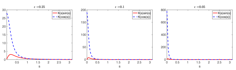
Figure 3: Plots of $K(s,t)\sin(s)$ (red solid) and $K(z,t)=K(\cos(s),t)$ (blue dashed) for the case in which the boundary is the unit sphere for different values of $\varepsilon\ell$ ($\ell=1$). For the unit sphere, we have $K(s,t)\sin(s)=K(s)\sin(s)=(2\varepsilon-\varepsilon^{2})\sin(s)\left[2(1-\varepsilon)(1-\cos s)+\varepsilon^{2}\right]^{-3/2}$ and $K(z,t)=K(z)=(2\varepsilon-\varepsilon^{2})\left[2(1-\varepsilon)(1-z)+\varepsilon^{2}\right]^{-3/2}$.

4.2 Local analysis of the single-layer potential

We now study the asymptotic behavior of $V^{\delta}(y^{\star};\varepsilon)$ as $\varepsilon\to 0^{+}$. The steps that we take here follow those used above for $U^{\delta}(y^{\star};\varepsilon)$. In particular, we introduce the stretched coordinate $s=\varepsilon S$ and find that the kernel in (4.4), which we denote by $G$, has the leading behavior,

$$G(\varepsilon S,t;\varepsilon)=\frac{J(\varepsilon S,t)}{|y_{d}(\varepsilon S,t)-\varepsilon\ell\tilde{n}(0,\cdot)|}=\frac{J(0,\cdot)}{\varepsilon(S^{2}|y_{s}(0,\cdot)|^{2}+\ell^{2})^{1/2}}+O(1).$$ (4.15)

In the limit as $\varepsilon\to 0^{+}$, we find that $G=O(\varepsilon^{-1})$ which characterizes its nearly singular behavior. Just as with the double-layer potential, we find that the leading behavior of this kernel is independent of $t$ and hence is azimuthally invariant about $y^{\star}$. When we substitute $s=\varepsilon S$ into (4.4) and replace $G$ by its leading behavior given in (4.15), we find after integrating with respect to $t$,

$$V^{\delta}(y^{\star};\varepsilon)=\frac{1}{2}J(0,\cdot)\tilde{\rho}(0,\cdot)\int_{0}^{\delta/\varepsilon}\frac{\varepsilon S}{(S^{2}|y_{s}(0,\cdot)|^{2}+\ell^{2})^{1/2}}\,\mathrm{d}S+O(\varepsilon^{2})\,.$$ (4.16)

In the asymptotic limit corresponding to $0<\varepsilon\ll\delta\ll 1$, we find that

$$\int_{0}^{\delta/\varepsilon}\frac{\varepsilon S}{(S^{2}|y_{s}(0,\cdot)|^{2}+\ell^{2})^{1/2}}\,\mathrm{d}S=\delta\frac{1}{|y_{s}(0,\cdot)|}+O(\varepsilon)\,.$$ (4.17)

It follows that

$$V^{\delta}(y^{\star};\varepsilon)=\delta\frac{1}{2}\frac{J(0,\cdot)\tilde{\rho}(0,\cdot)}{|y_{s}(0,\cdot)|}+O(\varepsilon).$$ (4.18)

In contrast to $U^{\delta}$, we find that the leading order behavior gives $V^{\delta}(y^{\star};\varepsilon)=O(1)$ as $\varepsilon\to 0^{+}$.
For the same reasons as discussed above for the double-layer potential, one finds that $G(s,t)\sin(s)$ is a smoother integrand than $G(z,t)=G(\cos(s),t)$. In Fig. 4 we present an example for the case of the unit sphere. Once again, this observation leads us to choose the substitution, $z=\frac{2}{\pi}s-1$.

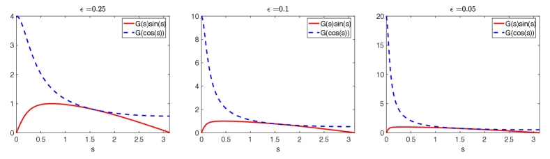
Figure 4: Plots of $G(s,t)\sin(s)$ (red solid) and $G(z,t)=G(\cos(s),t)$ (blue dashed) for the case in which the boundary is the unit sphere for different values of $\varepsilon\ell$ ($\ell=1$). For the unit sphere, we have $G(s,t)\sin(s)=G(s)\sin(s)=\sin(s)\left[2(1-\varepsilon)(1-\cos s)+\varepsilon^{2}\right]^{-1/2}$ and $G(z,t)=G(z)=\left[2(1-\varepsilon)(1-z)+\varepsilon^{2}\right]^{-1/2}$.

4.3 Results from this local analysis

The contribution by $B_{\delta}$ to (2.4) is given by

$$u^{\delta}(y^{\star}-\varepsilon\ell n^{\star})=u(y^{\star})-U^{\delta}(y^{\star};\varepsilon)+V^{\delta}(y^{\star};\varepsilon).$$ (4.19)

Using the results for the leading behaviors of $U^{\delta}$ and $V^{\delta}$ from above, we expect the error made by the leading behavior of $U^{\delta}$ given by (4.12) to be $O(\varepsilon^{2})$ and the error made by the leading behavior of $V^{\delta}$ given by (4.18) to be $O(\varepsilon)$. Consequently, the error made by the leading behavior of $u^{\delta}$ is $O(\varepsilon)$.

The asymptotic behavior computed above provides valuable insight into developing an accurate numerical method for (2.4). For any numerical integration method used to compute (2.4) at close evaluation points, large errors are likely to occur when the normal distance from $B$, given by $\varepsilon\ell$, is smaller than the fixed discretization length, $\pi/N$, see PGQ in Fig. 2. In that case, the kernels become sharply peaked about $y^{\star}$ which cannot be adequately resolved on the fixed boundary mesh.

The local analysis above indicates that it is advantageous in this setting to consider: (i) a rotated spherical coordinate system defined with respect to $y^{\star}$ that enhances the asymptotic behavior of the double- and single-layer potentials, and (ii) the use of the spherical Jacobian on the unit sphere, $\sin(s)$, explicitly that yields a smoother integrand. Following the above guidelines, one can guarantee an approximation of (2.4) that converges linearly with respect to distance from the boundary, $\varepsilon$, for a fixed resolution, $N$.

5 Numerical method for the close evaluation of layer potentials

We present a new numerical method for computing (2.4) that makes use of the results from the the asymptotic analysis in Section 4. By rotating the integrals as described above, azimuthal integration in this rotated coordinate system will naturally achieve the averaging operation that reveals the asymptotic behavior of the layer potentials. Recall, to rotate the integrals in this way, we apply the tranformation matrix described in A. The result of this rotation leads to

$$I(y^{\star})=\frac{1}{4\pi}\int_{-\pi}^{\pi}\int_{0}^{\pi}{F}(s,t)\sin(s)\,\mathrm{d}s\mathrm{d}t,$$ (5.1)

with

$${F(s,t)=-\frac{\tilde{n}(s,t)\cdot(y(0,\cdot)-y(s,t)-\varepsilon\ell n^{\star})}{|y(0,\cdot)-y(s,t)-\varepsilon\ell n^{\star}|^{3}}J(s,t)\left[\tilde{\mu}(s,t)-\tilde{\mu}(0,\cdot)\right]+\frac{1}{|y(0,\cdot)-y(s,t)-\varepsilon\ell n^{\star}|}J(s,t)\tilde{\rho}(s,t)}\,.$$ (5.2)

Since the local analysis also benefited from the explicit consideration of the factor of $\sin(s)$ appearing in the integral, compare (2.5) with (5.1), we choose to integrate with respect to the polar angle $s$ rather than the cosine of the polar angle as is typically done. Let $z_{i}\in(-1,1)$ for $i=1,\cdots,N$ denote the $N$-point Gauss-Legendre quadrature rule abscissas with corresponding weights, $w_{i}$ for $i=1,\cdots,N$. Let $t_{j}=-\pi+\pi(j-1)/N$ for $j=1,\cdots,2N$ denote an equi-spaced grid for $t\in[-\pi,\pi]$ for the periodic trapezoid rule. To compute (5.1) numerically, we introduce the substitution $s_{i}=\pi(z_{i}+1)/2$ for $i=1,\cdots,N$ and use the following quadrature rule,

$$I(y^{\star})\approx I^{N}(y^{\star})=\frac{\pi}{8N}\sum_{i=1}^{N}\sum_{j=1}^{2N}w_{i}\sin(s_{i})F(s_{i},t_{j}).$$ (5.3)

In (5.3) a factor of $\pi/2$ appears due to the scaling of the quadrature weights, $w_{i}$ for $i=1,\cdots,N$, that is required for the substitution from $z$ to $s$.

The quadrature rule given in (5.3) is a modification of the PGQ rule by Atkinson [3] presented in Section 3. There are two factors that make integrating with respect to $s$ more effective than integrating with respect to $\cos(s)$: (1) the inclusion of the factor $\sin(s)$ effectively smooths the peaks of the kernels in the double- and single-layer potentials about $s=0$ and (2) mapping the Gauss-Legendre points from $(-1,1)$ to $(0,\pi)$ clusters the quadrature points about $s=0$ where the kernels for the double- and single-layer potentials are peaked. In Fig. 5, we compare $s_{i}=\pi(z_{i}+1)/2$, $i=1,\dots,64$, denoted $O(\varepsilon)$, and $\cos^{-1}(z_{i})$, the PGQ method presented in Section 3, where $z_{i}$ are the $64$-point Gauss-Legendre quadrature abscissas. The two other quadrature methods presented in Section 3, SINH and IMT, are designed to effectively cluster points near $s=0$ to resolve the nearly singular behavior. We also include the SINH and IMT abscissas in Fig. 5. The new method and the IMT quadrature cluster in a similar way, while the SINH quadrature points cluster more, and the PGQ points do not cluster, as expected. Note that since the SINH abscissas depend on $\varepsilon$, one moderate choice, $\varepsilon=10^{-7}$, is presented here. To develop a method that successfully clusters to resolve these integrals, the nearly peaked region should have more quadrature points, yet not too many points should be removed from other regions. Observe that the SINH method is decreasing resolution quite significantly away from the peaked region and this leads to larger errors than IMT, as shown in Fig. 2B. We have chosen to use the Gauss-Legendre quadrature points in our method, based on PGQ, but one could also choose to use the IMT quadrature points with the mapping we suggest, $s_{i}=\pi(z_{i}+1)/2$. We choose to modify the PGQ as that is a commonly used quadrature and does not require a tabulation as IMT quadrature does.

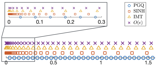
Figure 5: Comparison of the abscissas for PGQ, SINH quadrature, IMT quadrature, and our new method, denoted $O(\varepsilon)$. Each method has a resolution of $N=64$ between $0$ and $\pi$. Here, we present the quadrature points from $[0,\pi/2]$. and show a close up from $[0,0.3]$. The abscissas location for the SINH quadrature is dependent on $\varepsilon$ and we choose $\varepsilon=10^{-7}$ to show here.

We also note that since the Gauss-Legendre quadrature is an open rule, it does not include the end points $z=\pm 1$. Consequently, the mapping $s=\pi(z+1)/2$ does not include the end points $s=0$ and $s=\pi$. Therefore, the quadrature rule (5.3) does not require the explicit computation of $F(0,\cdot)$ which is the peak responsible for the nearly singular nature of this integral.

The quadrature rule given in (5.3) is effective for computing (2.4) because it excludes the need to evaluate the function to be integrated at its peak, smoothes the integrand (vanishing at the close evaluation point), clusters the quadrature points near the peaked behavior, and also includes the correct averaging operation introduced by azimuthal integration in the rotated coordinate system. Naively implementing this method to approximate the representation formula (2.4) for one evaluation point has the same computational cost as the PGQ method, $O(N^{2})$. This is quite expensive, especially due to the rotation that is required for these methods. We have not focused in this paper on fast implementations but do believe that it is possible to speed up this method using ideas that have been previously developed including the fast multipole method [20], the spherical grid rotations of Gimbutas and Veerapaneni [18], and considering surface patches rather than the entire surface.

6 Extension to $O(\varepsilon^{2})$

When quadrature rule (5.3) is adequately resolved for $F$ defined in (5.2), we expect it to exhibit an $O(\varepsilon)$ error in the limit as $\varepsilon\to 0^{+}$, consistent with the local analysis presented in Section 4. To obtain a smaller error, we need to address the $O(\varepsilon)$ error produced by the single-layer potential. Instead of considering the single-layer potential directly, we consider the asymptotic approximation,

$$\frac{1}{4\pi}\int_{B}\frac{\rho(y)}{|y^{\star}-y-\varepsilon\ell n^{\star}|}\,\mathrm{d}\sigma_{y}=\frac{1}{4\pi}\int_{B}\frac{\rho(y)}{|y^{\star}-y|}\,\mathrm{d}\sigma_{y}+\varepsilon\ell\frac{1}{4\pi}\int_{B}\frac{n^{\star}\cdot(y^{\star}-y)}{|y^{\star}-y|^{3}}\rho(y)\,\mathrm{d}\sigma_{y}-\frac{\varepsilon\ell}{2}\rho(y^{\star})+O(\varepsilon^{2})\,,$$ (6.1)

resulting from expanding the single-layer potential about $\varepsilon=0$, and using the boundary integral equation [21],

$$\frac{1}{4\pi}\frac{\partial}{\partial{n^{\star}}}\int_{B}\frac{\rho(y)}{|y^{\star}-y|}\,\mathrm{d}\sigma_{y}=-\frac{1}{2}\rho(y^{\star})+\frac{1}{4\pi}\int_{B}\frac{n^{\star}\cdot(y^{\star}-y)}{|y^{\star}-y|^{3}}\rho(y)\,\mathrm{d}\sigma_{y}.$$

The asymptotic approximation given in (6.1) is a sum of weakly singular integrals defined on $B$. Unlike the double-layer potential, the single-layer potential is continuous as $\varepsilon\to 0^{+}$. We consider (2.4) with the single-layer potential replaced with (6.1),

$$u(y^{\star}-\varepsilon\ell n^{\star})=u(y^{\star})-\frac{1}{4\pi}\int_{B}\frac{n(y)\cdot(y^{\star}-y-\varepsilon\ell n^{\star})}{|y^{\star}-y-\varepsilon\ell n^{\star}|^{3}}\left[\mu(y)-\mu(y^{\star})\right]\mathrm{d}\sigma_{y}\\ +\frac{1}{4\pi}\int_{B}\frac{1}{|y^{\star}-y|}\rho(y)\,\mathrm{d}\sigma_{y}+\varepsilon\ell\frac{1}{4\pi}\int_{B}\frac{n^{\star}\cdot(y^{\star}-y)}{|y^{\star}-y|^{3}}\rho(y)\,\mathrm{d}\sigma_{y}-\frac{\varepsilon\ell}{2}\rho(y^{\star}){+O(\varepsilon^{2})}.$$ (6.2)

To compute a numerical approximation of the integrals in (6.2), we apply the same quadrature rule described in Section 5 to the function

$${F(s,t)=-\frac{\tilde{n}(s,t)\cdot(y(0,\cdot)-y(s,t)-\varepsilon\ell n^{\star})}{|y(0,\cdot)-y(s,t)-\varepsilon\ell n^{\star}|^{3}}J(s,t)\left[\tilde{\mu}(s,t)-\tilde{\mu}(0,\cdot)\right]}\\ {+\frac{1}{|y(0,\cdot)-y(s,t)|}J(s,t)\tilde{\rho}(s,t)+\varepsilon\ell\frac{n^{\star}\cdot\left[y(0,\cdot)-y(s,t)\right]}{|y(0,\cdot)-y(s,t)|^{3}}J(s,t)\tilde{\rho}(s,t)\,.}$$ (6.3)

Provided that quadrature rule (5.3) is adequately resolved for (6.3), we expect it to exhibit an $O(\varepsilon^{2})$ error as $\varepsilon\to 0^{+}$.

7 Numerical results

We present numerical results for the solution of Laplace’s equation using representation formula (2.1) for close evaluation points. The new numerical method, detailed in Section 5, is used to solve the formulas given in (2.4) or (6.2). We consider exact solution (3.4), and proceed as in Section 3.

We test our method using two domains presented in Atkinson [4, 5]: (1) the peanut-shaped domain, given by (3.2) and (3.3) and (2) a mushroom cap domain given by (3.2) where

$$r(\theta)=2-\frac{1}{1+100(1-\cos\theta)^{2}}.$$ (7.1)

In the results that follow, we have set $\ell=1$ for both of these domains.

7.1 Results for peanut-shaped domain

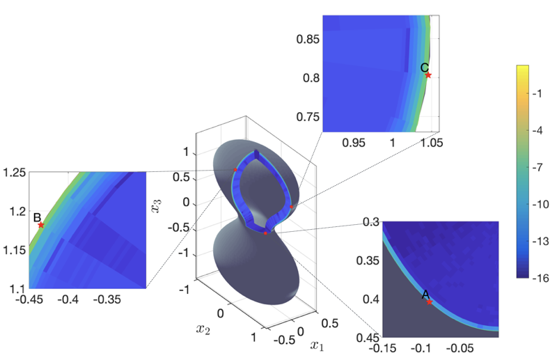
Figure 6: The logarithmic error for the new numerical method with $N=128$ applied to (2.4) when solving the close evaluation problem interior of the peanut-shaped domain. We have zoomed in around three points, A: $(-0.0894,0.4040,0)$, B: $(-0.4349,0,1.1819)$, and C: $(0,1.0456,0.8032)$. Further data for these three points is shown in Figs. 7 and 8.

In Fig. 6, we present the error interior of the peanut-shaped domain when using our newly developed numerical method with $N=128$ to approximate (2.4) with the expectation of $O(\varepsilon)$ error. In Fig. 7 and Fig. 8 we present the error as a function of $\varepsilon$ for this $O(\varepsilon)$ method compared to the three prior methods that were introduced in Section 3, the PGQ method, SINH method, and IMT method, starting at the three points (A, B, and C) labeled in Fig. 6. In Fig. 7, all four methods use $N=128$ and in Fig. 8, all methods use $N=256$. We observe that in all cases our method is $O(\varepsilon)$ as $\varepsilon\rightarrow 0^{+}$, as expected. Notably, this is even true for a moderate resolution of $N=128$. Also, we note that in the case of higher resolution, $N=256$, our method still has less error than all of the other three methods and further, the new method is the only one that has a consistent convergent behavior as $\varepsilon\rightarrow 0^{+}$.

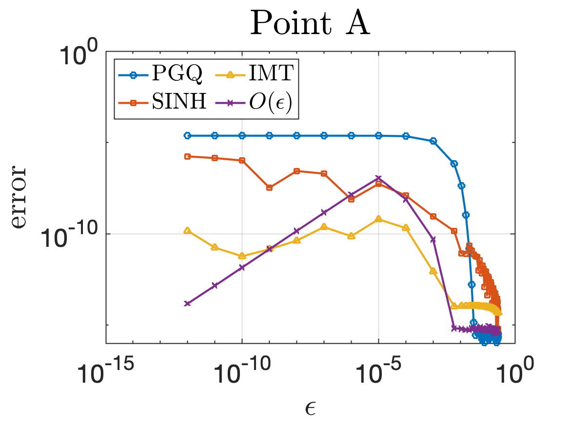
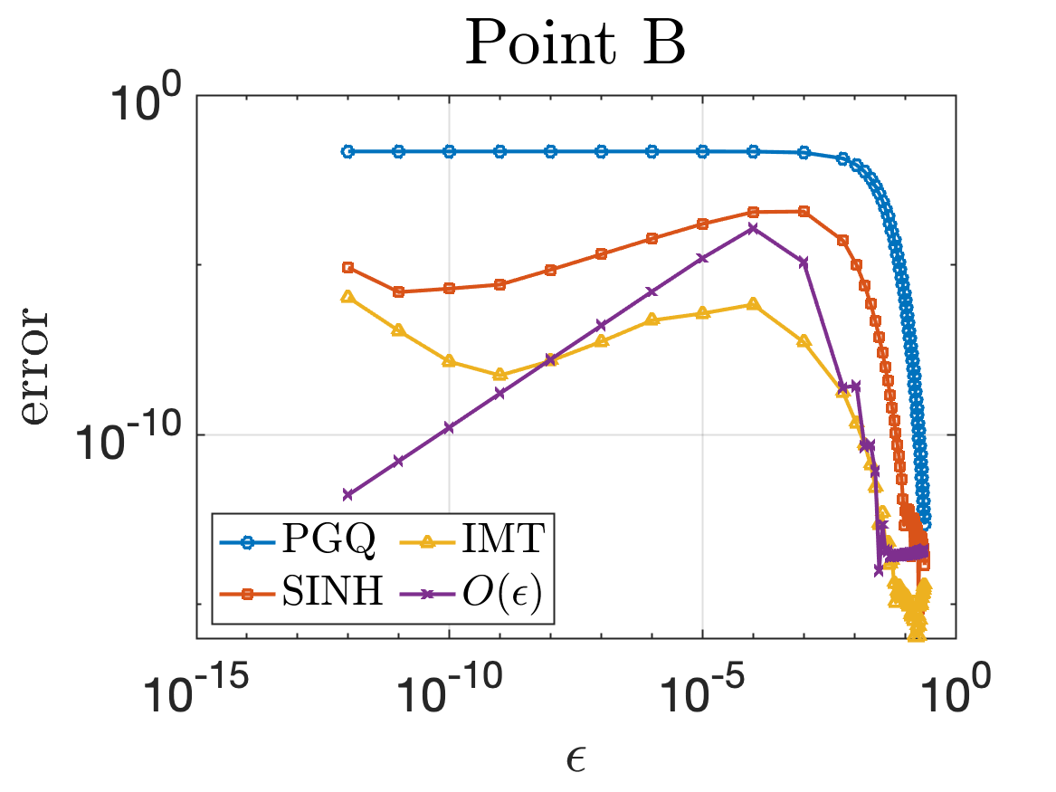
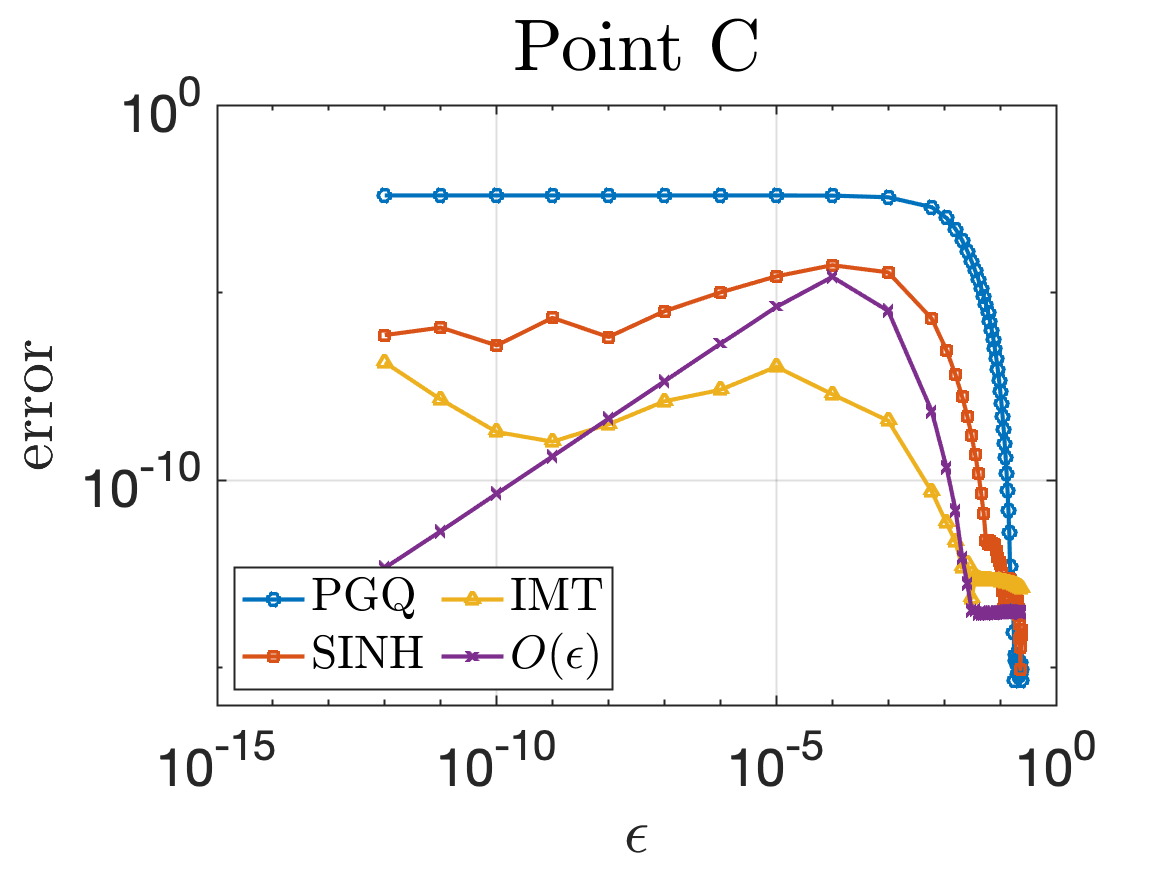
Figure 7: The logarithmic error for the new numerical method applied to (2.4) ($O(\varepsilon)$), PGQ method, SINH method, and IMT method with $N=128$ at the three zoomed in points, A, B, and C of Fig. 6 when solving the close evaluation problem interior of the peanut-shaped domain as a function of $\varepsilon$.

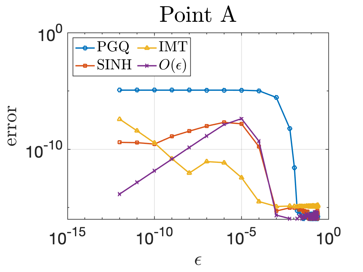
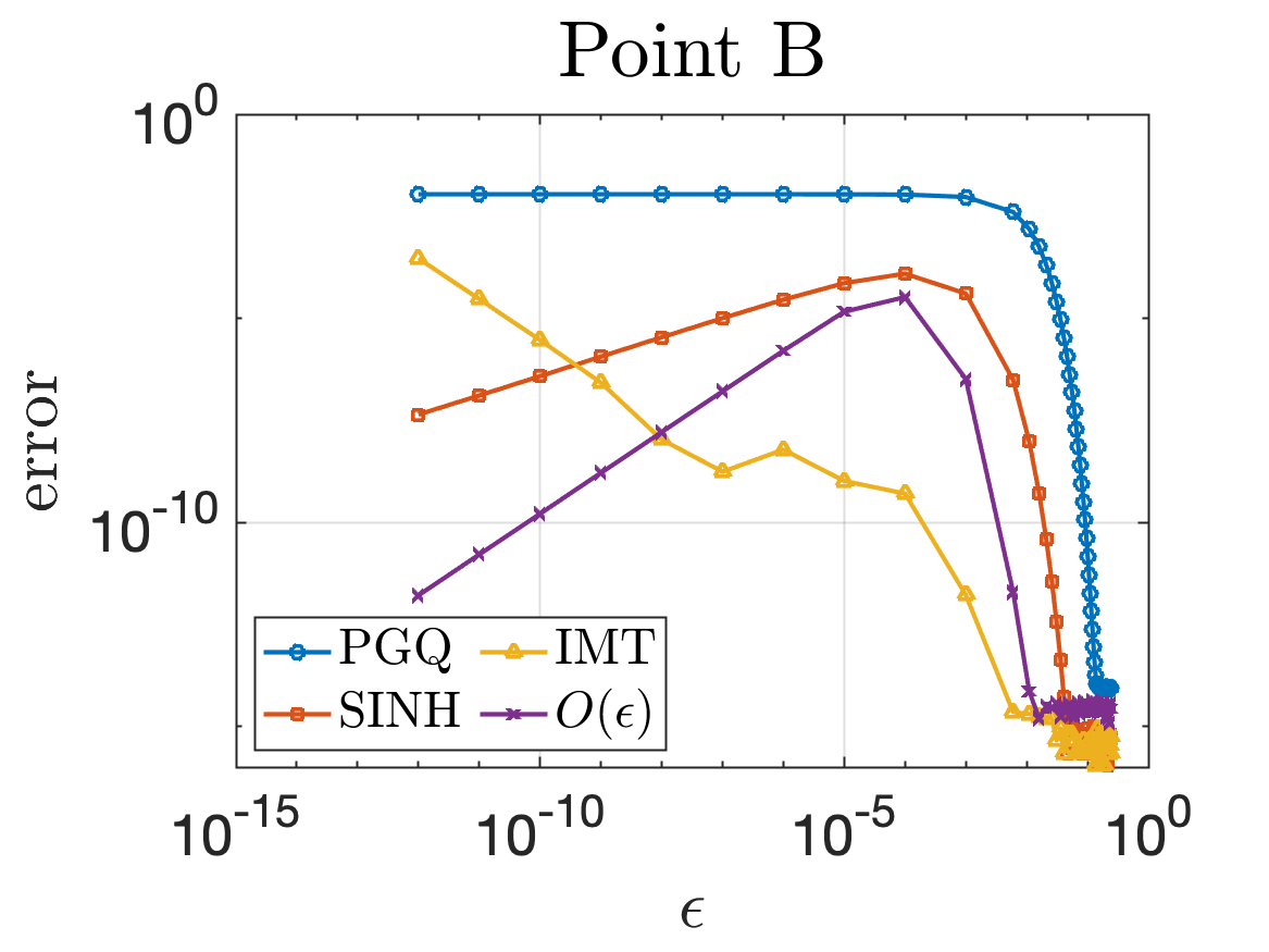
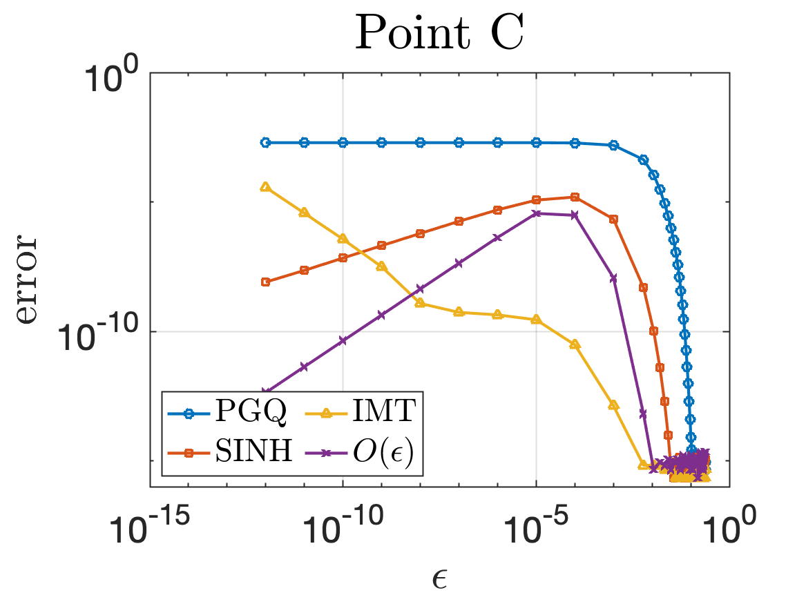
Figure 8: The logarithmic error for the new numerical method applied to (2.4) ($O(\varepsilon)$), PGQ method, SINH method, and IMT method with $N=256$ at the three zoomed in points, A, B, and C of Fig. 6 when solving the close evaluation problem interior of the peanut-shaped domain as a function of $\varepsilon$.

7.2 Results for mushroom cap domain

We now show the same analysis within the mushroom cap domain. In Fig. 9, we present the error interior of the mushroom cap domain when using the new numerical method with $N=128$ to approximate (2.4) In Fig. 10 we present the error as a function of $\varepsilon$ for all four methods starting at the three points (A, B, and C) labeled in Fig. 9. Once again, we observe, as expected, that our new method has an $O(\varepsilon)$ error as $\varepsilon\rightarrow 0^{+}$.

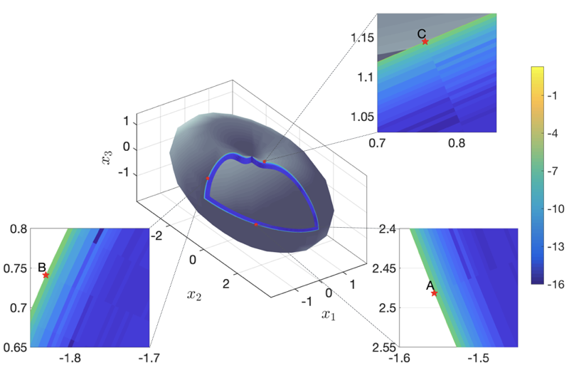
Figure 9: The logarithmic error for the new numerical method with $N=128$ applied to (2.4) when solving the close evaluation problem interior of the mushroom cap domain. We have zoomed in around three points, A: $(-1.5559,2.4816,0)$, B: $(-1.8307,0,0.7412)$, and C: $(0,0.7601,1.1446)$. Further data for these three points is shown in Fig. 10.

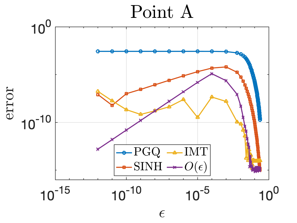
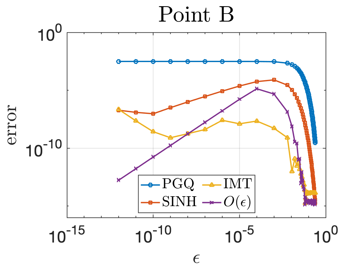
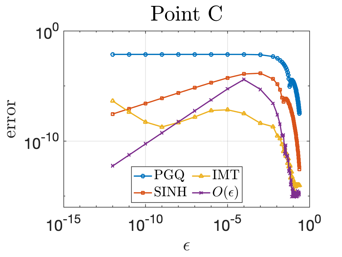
Figure 10: The logarithmic error for the new numerical method applied to (2.4) ($O(\varepsilon)$), PGQ method, SINH method, and IMT method with $N=128$ at the three zoomed in points, A, B, and C of Fig. 9 when solving the close evaluation problem interior of the mushroom cap domain as a function of $\varepsilon$.

7.3 Extension to $O(\varepsilon^{2})$

In this section, we present results of when the new numerical method, detailed in Section 5, is used to solve both (2.4), the $O(\varepsilon)$ method shown above, and (6.2). In the latter case, we expect the error to be $O(\varepsilon^{2})$ as $\varepsilon\rightarrow 0^{+}$.

In Fig. 11, we show the logarithmic error for both the $O(\varepsilon)$ method and the $O(\varepsilon^{2})$ method starting at the three $y^{\star}$ points (A, B, and C), labeled in Fig. 6, interior to the peanut-shaped domain with $N=128$. Similarly, in Fig. 12, we show the error of the two methods for the three points labeled in Fig. 9, interior to the mushroom cap domain. Observe that the numerical method applied to (6.2) has an $O(\varepsilon^{2})$ error as $\varepsilon\rightarrow 0^{+}$ and reaches machine precision for small $\varepsilon$. Note that this method is different from the $O(\varepsilon)$ method because it depends on an asymptotic expansion of the single-layer potential as $\varepsilon\rightarrow 0^{+}$ and therefore exhibits larger errors as $\varepsilon$ increases.

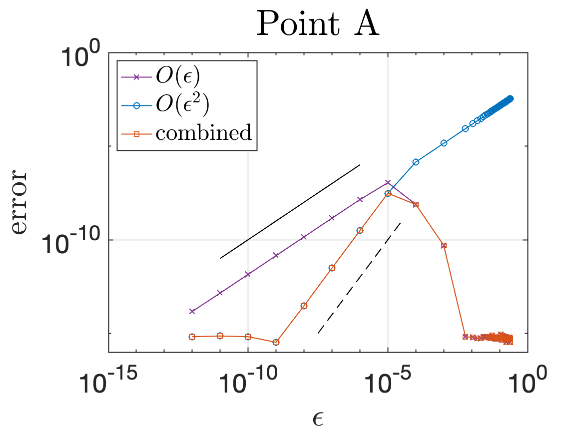
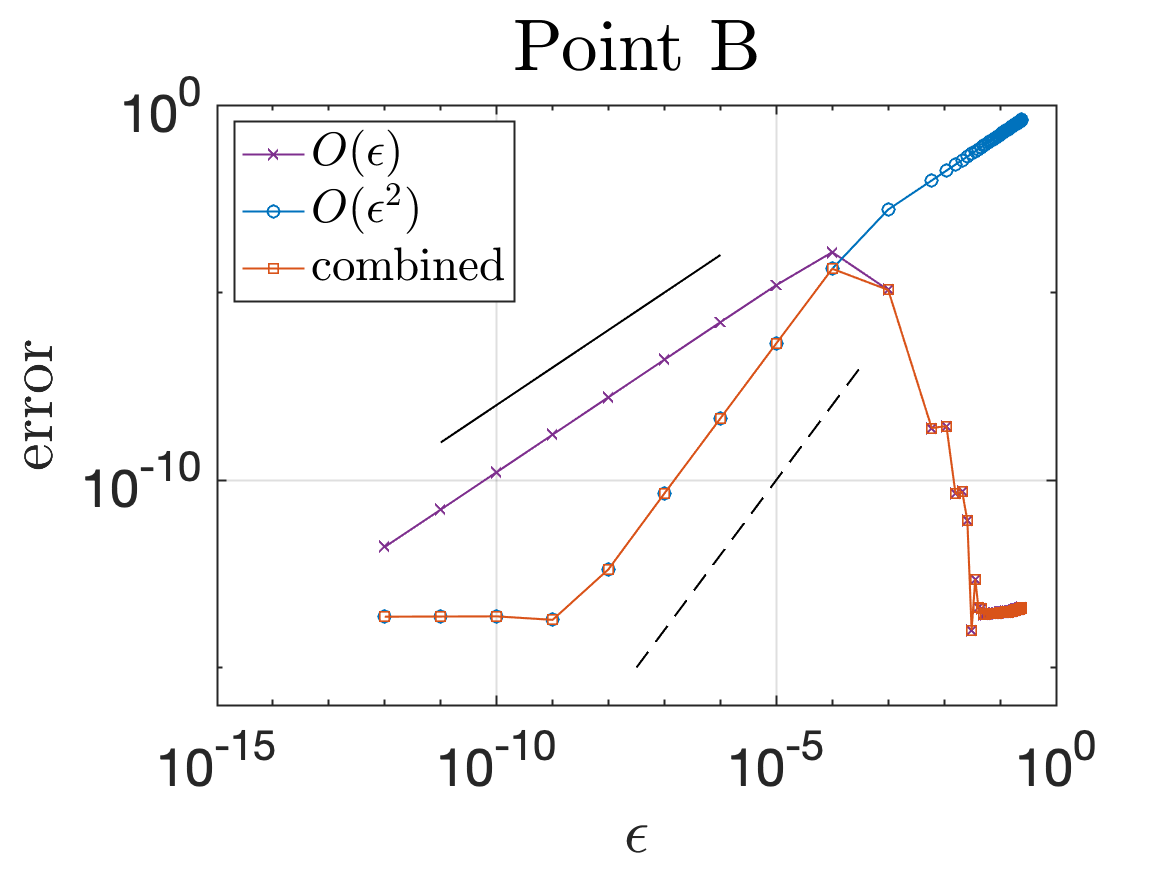
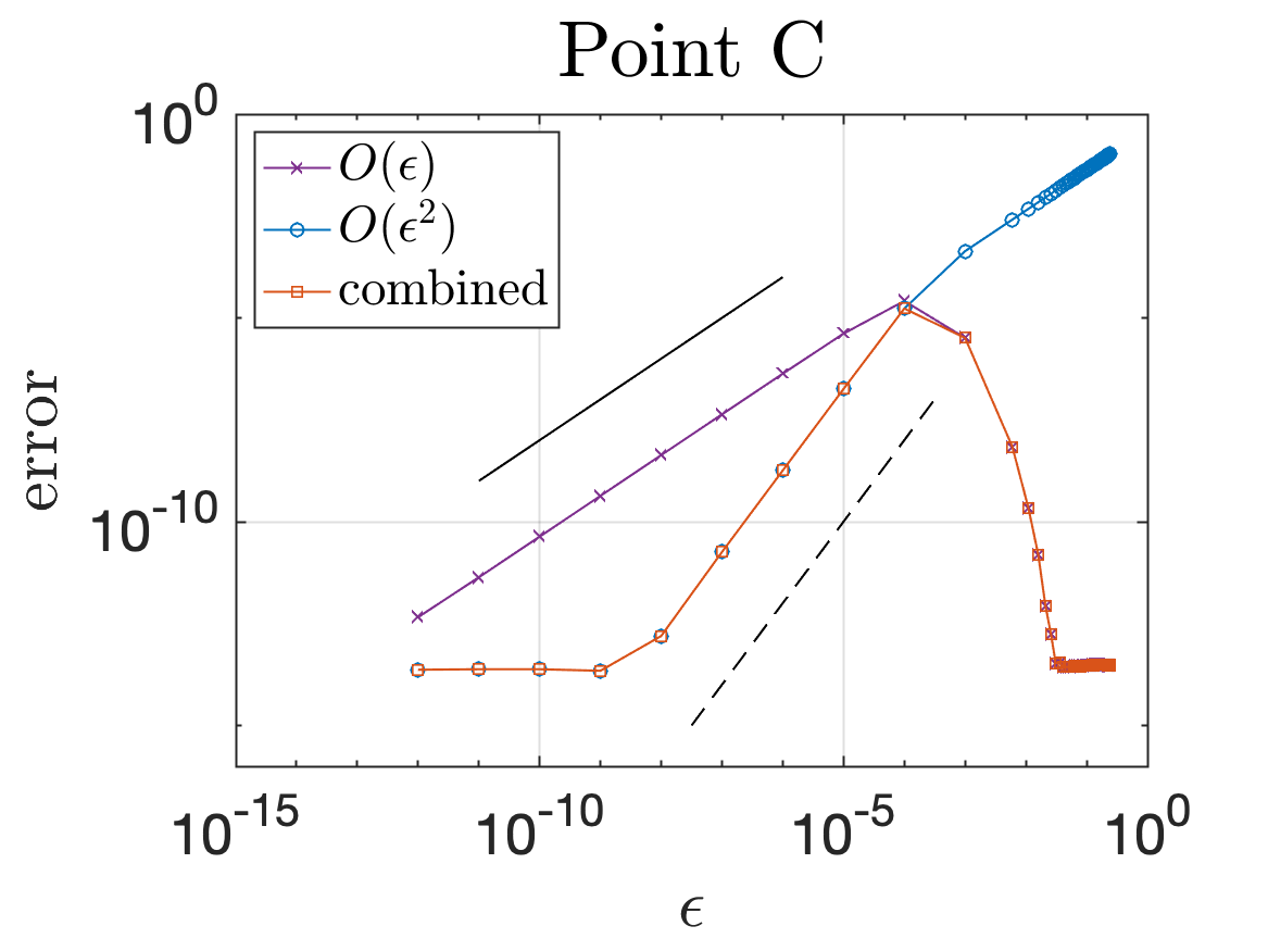
Figure 11: The logarithmic error for the new numerical method applied to (2.4) ($O(\varepsilon)$) and to (6.2) ($O(\varepsilon^{2})$) and the combined method with $N=128$ at the three zoomed in points, A, B, and C of Fig. 6 when solving the close evaluation problem interior of the peanut-shaped domain as a function of $\varepsilon$. The solid black line demonstrates $O(\varepsilon)$ convergence and the dashed black line demonstrates $O(\varepsilon^{2})$ convergence.

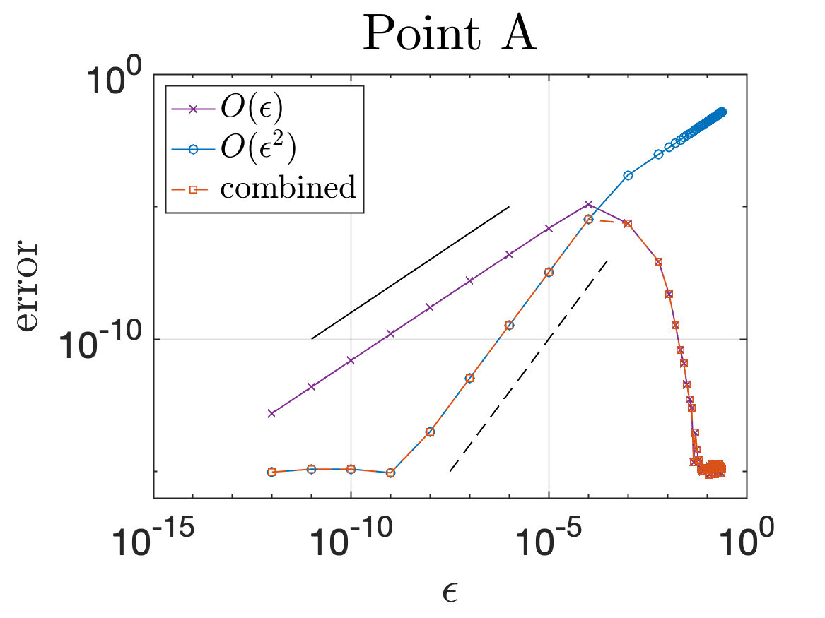
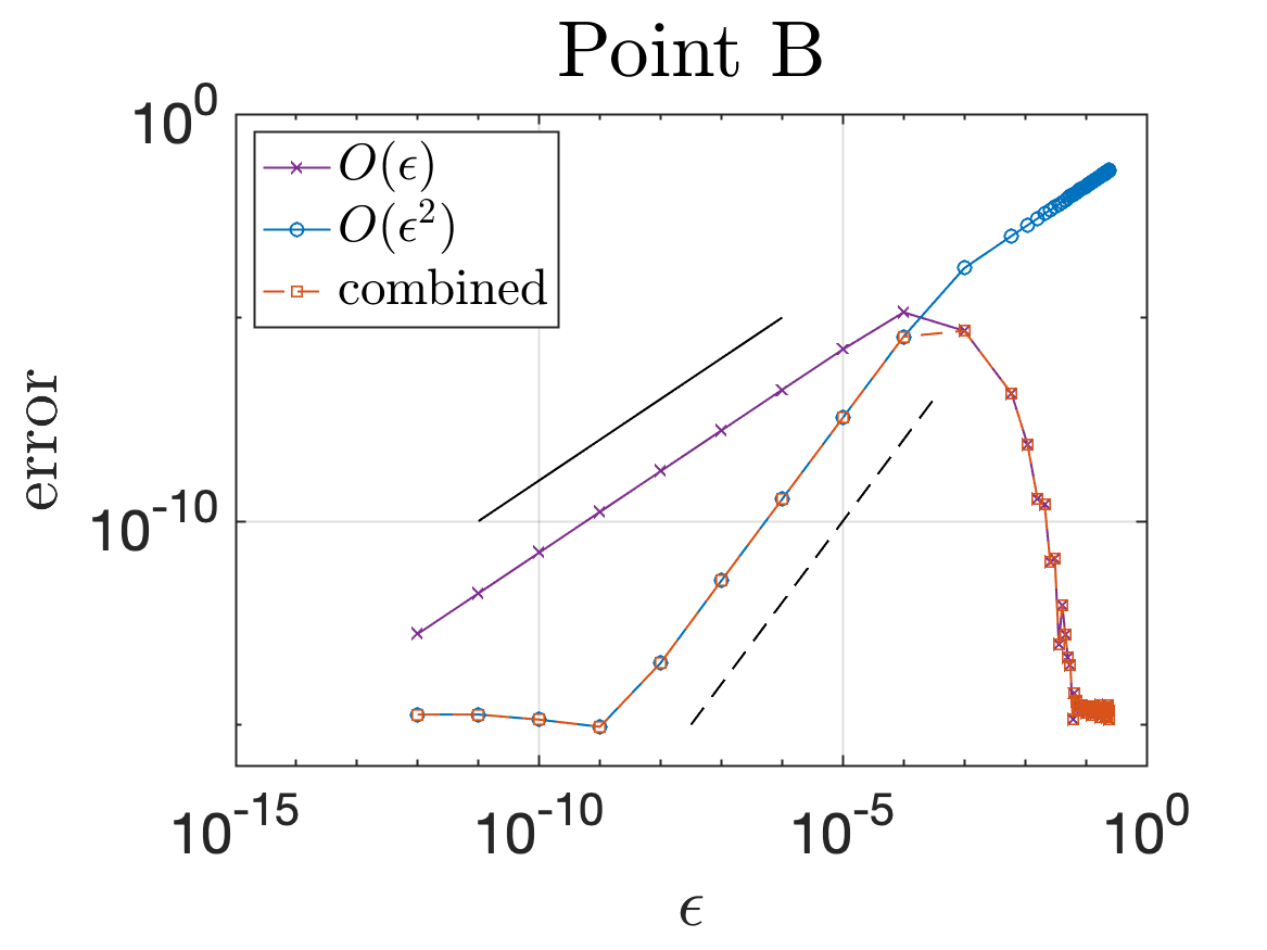
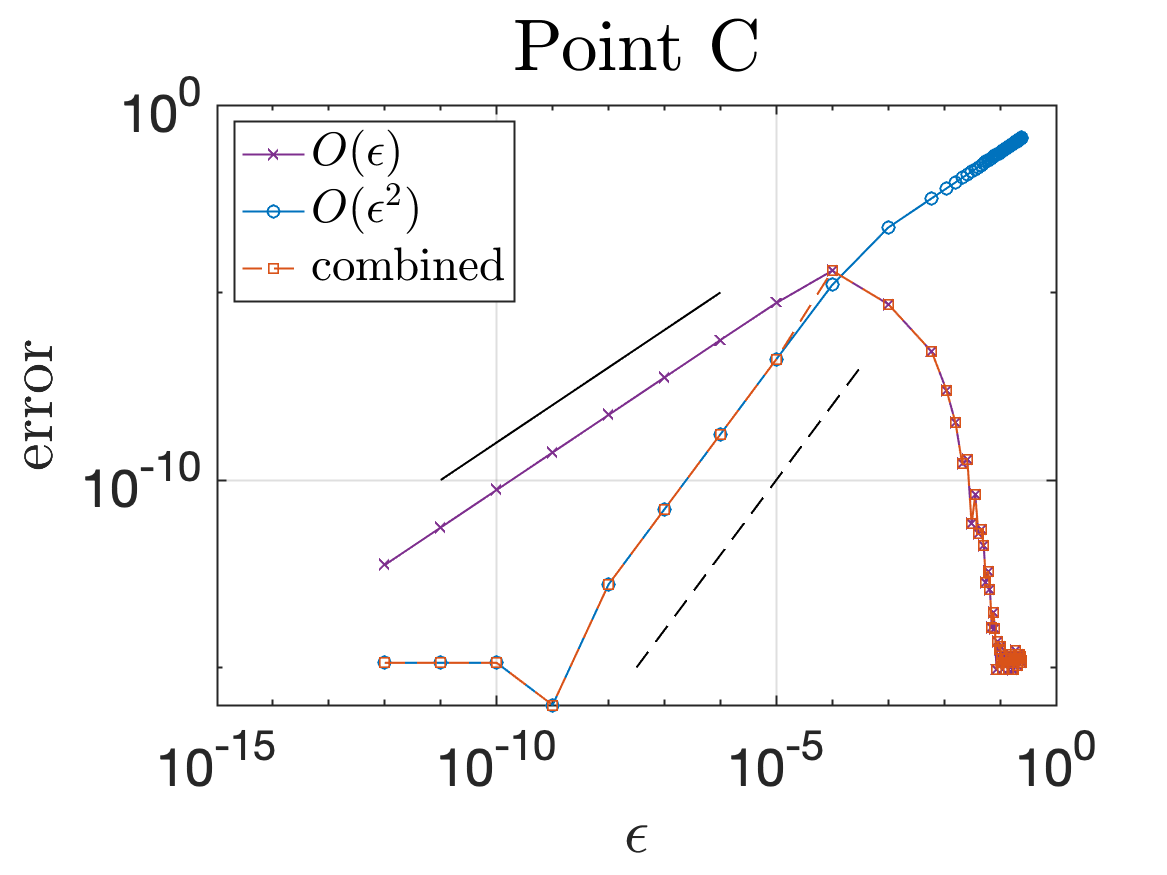
Figure 12: The logarithmic error for the new numerical method applied to (2.4) ($O(\varepsilon)$) and to (6.2) ($O(\varepsilon^{2})$) and the combined method with $N=128$ at the three zoomed in points, A, B, and C of Fig. 9 when solving the close evaluation problem interior of the mushroom cap domain as a function of $\varepsilon$. The solid black line demonstrates $O(\varepsilon)$ convergence and the dashed black line demonstrates $O(\varepsilon^{2})$ convergence.

Even though the focus of this work is to study the behavior of the close evaluation problem when using a fixed $N$-point quadrature and varying $\varepsilon$, we present in Fig. 13 the logarithmic error as both $\varepsilon$ and $N$ vary for the $O(\varepsilon)$ method and the $O(\varepsilon^{2})$ method at point B labeled in Fig. 6 for the peanut-shaped domain. Similarly, we present the logarithmic error as both $\varepsilon$ and $N$ vary for point B labeled in Fig. 9 for the mushroom cap domain. For both methods, $N$ must be large enough to resolve the domain to not observe $O(1)$ errors. As stated above, for the $O(\varepsilon^{2})$ method, since we have used an expansion for the single-layer potential, the method exhibits larger errors far from the boundary. For the newly developed methods here, once past a minimum $N$ value ($N\approx 100$ here), the error is constant in $N$ for small values of $\varepsilon$. This is expected for the numerical methods developed here based on our asymptotic analysis in $\varepsilon$, as presented in Section 4. Once again, we observe that the methods are $O(\varepsilon)$ and $O(\varepsilon^{2})$, as expected, and the $O(\varepsilon^{2})$ method reaches machine precision for small $\varepsilon$.

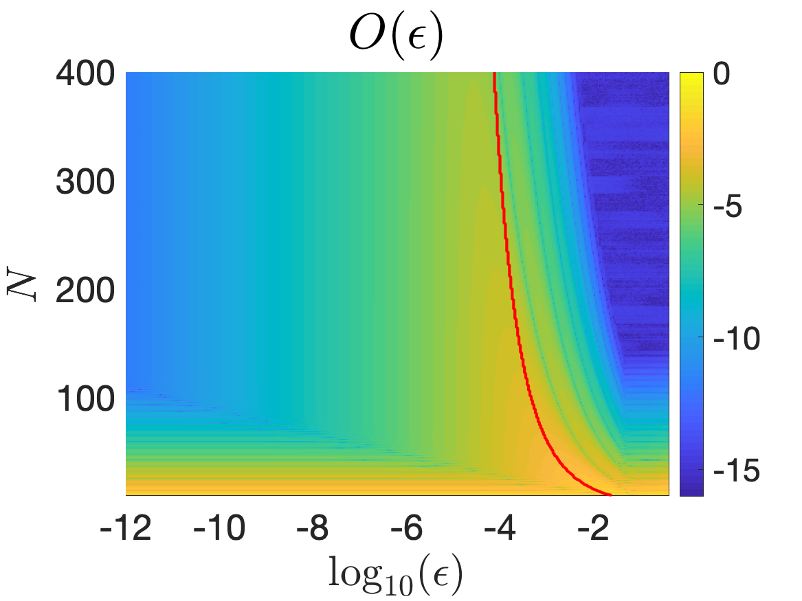
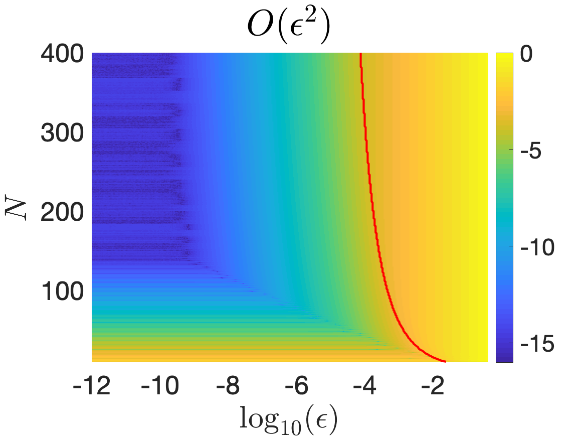
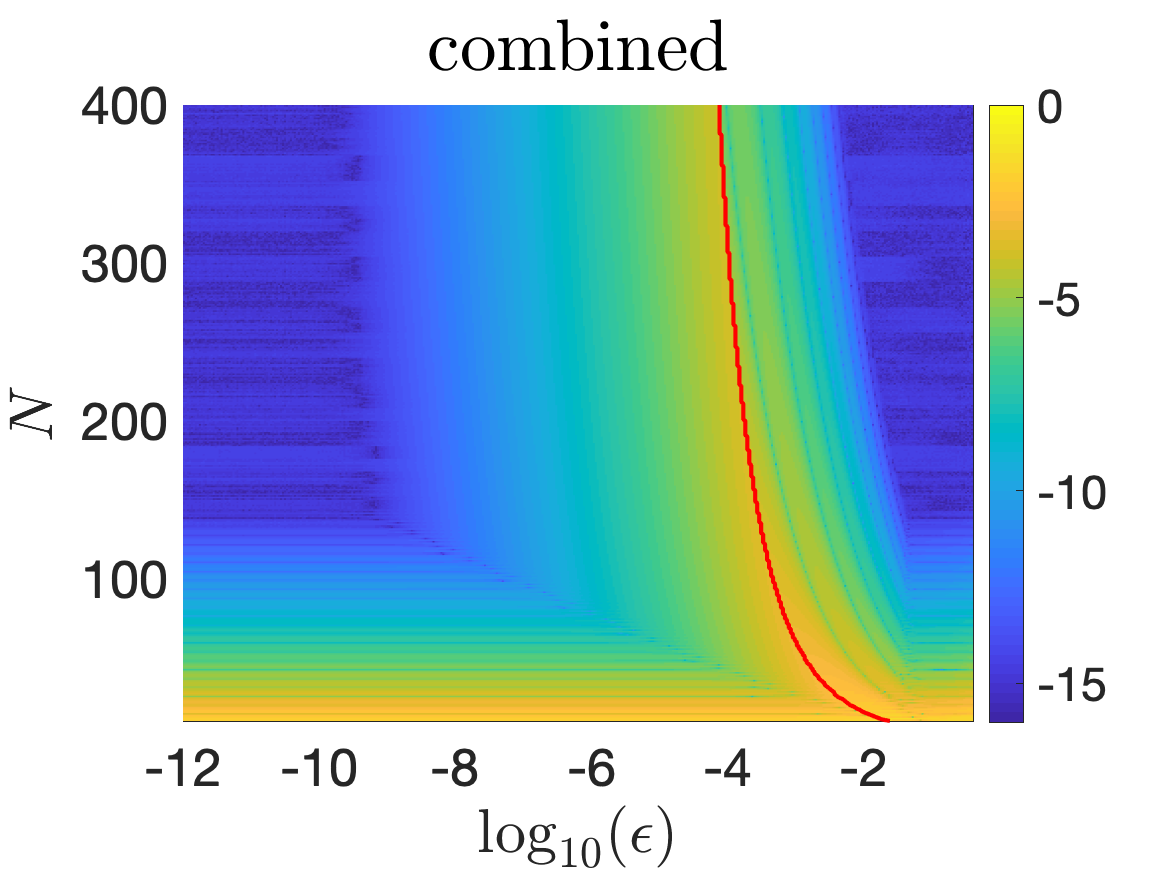
Figure 13: The logarithmic error for the $O(\varepsilon)$ method, the $O(\varepsilon^{2})$ method, and the combined method at the zoomed in point B of Fig. 6 when solving the close evaluation problem interior of the peanut-shaped domain as a function of $N$ and $\varepsilon$. The red curve on each plot shows where we switch from the $O(\varepsilon^{2})$ method to the $O(\varepsilon)$ method in the combined method.

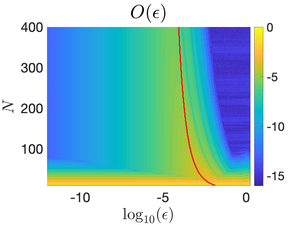
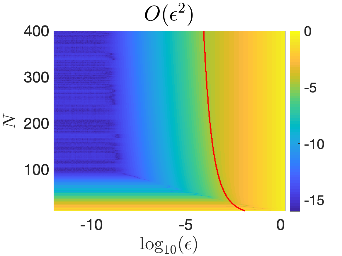
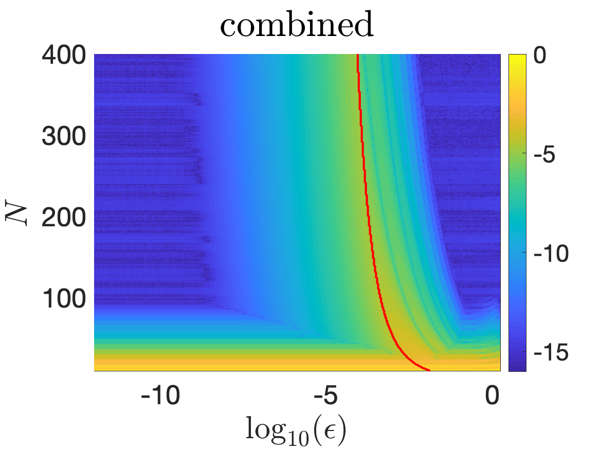
Figure 14: The logarithmic error for the $O(\varepsilon)$ method, the $O(\varepsilon^{2})$ method, and the combined method at the zoomed in point B of Fig. 9 when solving the close evaluation problem interior of the mushroom cap domain as a function of $N$ and $\varepsilon$. The red curve on each plot shows where we switch from the $O(\varepsilon^{2})$ method to the $O(\varepsilon)$ method in the combined method.

The optimized numerical method would combine the $O(\varepsilon^{2})$ method for the smallest values of $\varepsilon$ with the $O(\varepsilon)$ method for larger values. This combined method is also presented in Figs. 11 and 12 and in Figs. 13 and 14. To determine at which value of $\varepsilon$ to switch between methods, in particular in general cases when there is not a known exact solution, we extend an idea we developed in two dimensions [12] to three dimensions. For a fixed $y^{\star}$ and fixed resolution, $N$, we evaluate Gauss’ Law, (2.3), for varying $\varepsilon$ using the PGQ method and compute the error. This method will suffer from the close evaluation problem and the error approaches $O(1)$ as $\varepsilon\rightarrow 0^{+}$. We choose a tolerance for the error to Gauss’ Law, close to where it first approaches $O(1)$. In all cases presented in this paper, this tolerance was chosen to be $0.495$. This error tolerance then corresponds to an $\varepsilon$ value for the fixed $y^{\star}$ and fixed resolution, $N$, which is then used as the $\varepsilon$ value at which to switch between the two methods. In the plots in Figs. 13 and 14, the red curves give the $\varepsilon$ values for each $N$ at which we switch between the $O(\varepsilon^{2})$ method and the $O(\varepsilon)$ method in the combined method. We observe in Figs. 11 and 12 and in Figs. 13 and 14 that the $\varepsilon$ value at which we switch between the methods is the ideal value, allowing the combined method to benefit from the best of each of the $O(\varepsilon)$ and $O(\varepsilon^{2})$ methods.

7.4 Effect of Curvature

In the above results presented, we have focused on two domains, the peanut-shaped domain and the mushroom cap domain. It is well known that the curvature plays a role in the error observed in the close evaluation problem [7, 12]. Here, we present results to systematically study the robustness of the new method when considering curvature. We test our new method on four different domains, one sphere and three ellipsoids, as shown in Fig. 15,

$$y(\theta,\varphi)=(\sin\theta\cos\varphi,b\sin\theta\sin\varphi,\cos\theta),\quad\theta\in[0,\pi],\quad\varphi\in[-\pi,\pi],$$ (7.2)

where $b=1$ for the sphere and $b=2,4,8$ for the ellipsoids. In Fig. 15, we present the logarithmic error as a function of $\varepsilon$ starting at two values of $y^{\star}$ on each boundary, $(-1,0,0)$ (Point A) and $(0,b,0)$ (Point B) when using the combined method, as discussed above in Section 7.3. We observe that our new numerical is robust to variations in curvature and there is no appreciable difference in the errors as the curvature of the boundary increases.

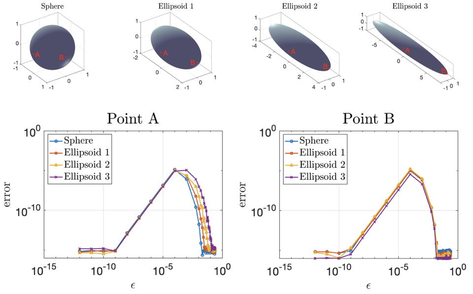
Figure 15: The logarithmic error for the new numerical method with $N=128$ when solving the close evaluation problem interior to four different domains, a sphere and three ellipsoids (top row) at two points, A: $(-1,0,0)$ and B: $(0,b,0)$ where $b=1,2,4$ or $8$.

7.5 Summary of the results

For both the peanut-shaped and mushroom cap domains, we have found that the new numerical method we have developed here provides the most accurate evaluation of the representation formula for close evaluation points exhibiting an error that is $O(\varepsilon^{2})$ as $\varepsilon\rightarrow 0^{+}$. The $O(\varepsilon)$ method is the next most accurate due to the increased error from the single-layer potential. These error results are expected based on the analysis provided in Section 4 and the extension given in Section 6. These results are consistent for two very different three-dimensional domains and robust when systematically studying the curvature of the boundary. Thus, these results demonstrate that the numerical method developed here is accurate and effective for the close evaluation problem.

8 Conclusions

We have presented a simple and effective numerical method for the close evaluation of double- and single-layer potentials in three dimensions. The close evaluation of these layer potentials are challenging to numerically compute because they are nearly singular integrals. Through a local analysis of the close evaluation of double- and single-layer potentials about the point at which their kernels are sharply peaked, we have identified a natural way to compute these nearly singular integrals.

Under the simplifying assumption that the boundary can be parameterized using spherical coordinates, we work in a rotated coordinate system in which the singular point maps to the north pole of a sphere. This rotated coordinate system highlights the axisymmetry of the kernels for the double- and single-layer potentials at close evaluation points. We then propose a numerical quadrature rule for the double- and single-layer potentials written in spherical coordinates. In this rotated coordinate system, azimuthal integration acts as a natural averaging operation about the singular point, which enhances its asymptotic behavior at close evaluation points. The quadrature rule also integrates over the polar angle directly rather than integrating over the cosine of the polar angle. By doing so, the numerical integration includes a factor of sine of the polar angle (the natural Jacobian for the spherical coordinate system) which is important for effectively computing these nearly singular integrals. Finally, because we use an open Gauss-Legendre quadrature rule for the polar angle, we do not require explicit evaluation of the kernels at the peaked points.

We have computed results for evaluating the representation formula interior to a boundary for two different domains and observed the expected behavior. Further, we have shown that our method is robust to variations in curvature through a systematic study. This method can easily be extended to evaluating the representation formula exterior to a boundary. One obtains these results by taking care of the outward normals in the formulas used throughout this discussion and in Gauss’ law.

We have assumed that the boundary is closed, oriented, and analytic in this paper. However, as long as a portion of the boundary about the singular point is sufficiently smooth and can be parameterized using spherical coordinates (in other words integrating over a cap of a sphere), these results hold. Thus, this method can be extended to finite-sized patches covering a surface [11, 29].

Finally, the analysis shown here can be extended to other problems. In particular, this method is broadly applicable to weakly singular and nearly singular integrals over two-dimensional surfaces. These weakly singular and nearly singular integrals may correspond to solutions of other elliptic partial differential equations including Helmholtz’s equation and the Stokes’ equations.

Appendix A Rotations on the sphere

We give the explicit rotation formulas over the sphere used throughout this paper. Consider $v,v^{\star}\in S^{2}$, with $S^{2}$ denoting the unit sphere. The $(\hat{\i},\hat{\j},\hat{{\rm k}})$-coordinate system corresponds to the laboratory reference frame. We introduce the parameters $\theta\in[0,\pi]$ and $\varphi\in[-\pi,\pi]$ and write

$$v=v(\theta,\varphi)=\sin\theta\cos\varphi\,\hat{\i}+\sin\theta\sin\varphi\,\hat{\j}+\cos\theta\,\hat{{\rm k}}.$$ (A.1)

The specific parameters $\theta^{\star}$ and $\varphi^{\star}$ are defined through the relation $v^{\star}=v(\theta^{\star},\varphi^{\star})$. We would like to work in the rotated, $(\hat{e}_{1},\hat{e}_{2},\hat{e}_{3})$-coordinate system in which

$$\hat{e}_{1} =\cos\theta^{\star}\cos\varphi^{\star}\,\hat{\i}+\cos\theta^{\star}\sin\varphi^{\star}\,\hat{\j}-\sin\theta^{\star}\,\hat{{\rm k}},$$ (A.2)

$$\hat{e}_{2} =-\sin\varphi^{\star}\,\hat{\i}+\cos\varphi^{\star}\,\hat{\j},$$

$$\hat{e}_{3} =\sin\theta^{\star}\cos\varphi^{\star}\,\hat{\i}+\sin\theta^{\star}\sin\varphi^{\star}\,\hat{\j}+\cos\theta^{\star}\,\hat{{\rm k}}.$$

In this rotated system we have $\hat{e}_{3}=v^{\star}$. For this rotated coordinate system, we introduce the parameters $s\in[0,\pi]$ and $t\in[-\pi,\pi]$ such that

$$v=v(s,t)=\sin s\cos t\,\hat{e}_{1}+\sin s\sin t\,\hat{e}_{2}+\cos s\,\hat{e}_{3}.$$ (A.3)

It follows that $\hat{e}_{3}=v^{\star}=v(0,\cdot)$. This corresponds to setting $v^{\star}$ to be the north pole of the rotated sphere. By equating (A.1) and (A.3) and substituting (A.2) into that result, we obtain

$$\begin{bmatrix}\sin\theta\cos\varphi\\ \sin\theta\sin\varphi\\ \cos\theta\end{bmatrix}=\begin{bmatrix}\cos\theta^{\star}\cos\varphi^{\star}&-\sin\varphi^{\star}&\sin\theta^{\star}\cos\varphi^{\star}\\ \cos\theta^{\star}\sin\varphi^{\star}&\cos\varphi^{\star}&\sin\theta^{\star}\sin\varphi^{\star}\\ -\sin\theta^{\star}&0&\cos\theta^{\star}\end{bmatrix}\begin{bmatrix}\sin s\cos t\\ \sin s\sin t\\ \cos s\end{bmatrix}.$$ (A.4)

Let us rewrite (A.4) compactly as $v(\theta,\varphi)=R(\theta^{\star},\varphi^{\star})v(s,t)$ with $R(\theta^{\star},\varphi^{\star})$ denoting the $3\times 3$ matrix given above. It is a rotation matrix. Hence, it is orthogonal.

We now seek to write $\theta=\theta(s,t)$ and $\varphi=\varphi(s,t)$. To do so, we introduce

$$\xi(s,t;\theta^{\star},\varphi^{\star}) =\cos\theta^{\star}\cos\varphi^{\star}\sin s\cos t-\sin\varphi^{\star}\sin s\sin t+\sin\theta^{\star}\cos\varphi^{\star}\cos s,$$ (A.5)

$$\eta(s,t;\theta^{\star},\varphi^{\star}) =\cos\theta^{\star}\sin\varphi^{\star}\sin s\cos t+\cos\varphi^{\star}\sin s\sin t+\sin\theta^{\star}\sin\varphi^{\star}\cos s,$$ (A.6)

$$\zeta(s,t;\theta^{\star},\varphi^{\star}) =-\sin\theta^{\star}\sin s\cos t+\cos\theta^{\star}\cos s.$$ (A.7)

From (A.5) - (A.7), we find that

$$\theta=\arctan\left(\frac{\sqrt{\xi^{2}+\eta^{2}}}{\zeta}\right),$$ (A.8)

and

$$\varphi=\arctan\left(\frac{\eta}{\xi}\right).$$ (A.9)

These results give the formulas needed to evaluate $\theta=\theta(s_{i},t_{j})$ and $\varphi=\varphi(s_{i},t_{j})$ that are used in Sections 3 and 5. This $\theta$ and $\phi$ are used to evaluate $y(s_{i},t_{j})=y(\theta(s_{i},t_{j}),\varphi(s_{i},t_{j}))$ using (3.2) or (7.2) in the quadrature rules (3.1) and (5.3).

References

- [1] L. af Klinteberg, A.-K. Tornberg, A fast integral equation method for solid particles in viscous flow using quadrature by expansion, J. Comput. Phys. 326 (2016) 420–445.
- [2] L. af Klinteberg, A.-K. Tornberg, Error estimation for quadrature by expansion in layer potential evaluation, Adv. Comput. Math. 43 (1) (2017) 195–234.
- [3] K. E. Atkinson, Numerical integration on the sphere, ANZIAM J. 23 (3) (1982) 332–347.
- [4] K. E. Atkinson, The numerical solution Laplace’s equation in three dimensions, SIAM J. Numer. Anal. 19 (2) (1982) 263–274.
- [5] K. E. Atkinson, Algorithm 629: An integral equation program for Laplace’s equation in three dimensions, ACM Trans. Math. Softw. 11 (2) (1985) 85–96.
- [6] K. E. Atkinson, The Numerical Solution of Integral Equations of the Second Kind, Cambridge University Press, 1997.
- [7] A. H. Barnett, Evaluation of layer potentials close to the boundary for Laplace and Helmholtz problems on analytic planar domains, SIAM J. Sci. Comput. 36 (2) (2014) A427–A451.
- [8] J. T. Beale, M.-C. Lai, A method for computing nearly singular integrals, SIAM J. Numer. Anal. 38 (6) (2001) 1902–1925.
- [9] J. T. Beale, W. Ying, J. R. Wilson, A simple method for computing singular or nearly singular integrals on closed surfaces, Commun. Comput. Phys. 20 (3) (2016) 733–753.
- [10] J. Bremer, Z. Gimbutas, V. Rokhlin, A nonlinear optimization procedure for generalized gaussian quadratures, SIAM J. Sci. Comput. 32 (4) (2010) 1761–1788.
- [11] O. P. Bruno, L. A. Kunyansky, A fast, high-order algorithm for the solution of surface scattering problems: basic implementation, tests, and applications, J. Comput. Phys. 169 (1) (2001) 80–110.
- [12] C. Carvalho, S. Khatri, A. D. Kim, Asymptotic analysis for close evaluation of layer potentials, J. Comput. Phys. 355 (2018) 327–341.
- [13] C. Carvalho, S. Khatri, A. D. Kim, Asymptotic approximations for the close evaluation of double-layer potentials, SIAM J. Sci. Comput. 42 (1) (2020) A504–A533.
- [14] L. M. Delves, J. L. Mohamed, Computational Methods for Integral Equations, Cambridge University Press, 1988.
- [15] C. L. Epstein, L. Greengard, A. Klöckner, On the convergence of local expansions of layer potentials, SIAM J. Numer. Anal. 51 (5) (2013) 2660–2679.
- [16] G. B. Folland, Introduction to partial differential equations, vol. 102, Princeton university press, 1995.
- [17] M. Ganesh, I. Graham, A high-order algorithm for obstacle scattering in three dimensions, J. Comput. Phys. 198 (1) (2004) 211–242.
- [18] Z. Gimbutas, S. Veerapaneni, A fast algorithm for spherical grid rotations and its application to singular quadrature, SIAM J. Sci. Comput. 35 (6) (2013) A2738–A2751.
- [19] I. G. Graham, I. H. Sloan, Fully discrete spectral boundary integral methods for Helmholtz problems on smooth closed surfaces in , Numerische Mathematik 92 (2) (2002) 289–323.
- [20] L. Greengard, V. Rokhlin, A new version of the Fast Multipole Method for the Laplace equation in three dimensions, Acta Numerica 6 (1997) 229–269.
- [21] R. B. Guenther, J. W. Lee, Partial Differential Equations of Mathematical Physics and Integral Equations, Dover Publications, 1996.
- [22] J. Helsing, R. Ojala, On the evaluation of layer potentials close to their sources, J. Comput. Phys. 227 (5) (2008) 2899–2921.
- [23] M. Iri, S. Moriguti, Y. Takasawa, On a certain quadrature formula, J. Comput. Appl. Math 17 (1-2) (1987) 3–20.
- [24] P. R. Johnston, D. Elliott, A sinh transformation for evaluating nearly singular boundary element integrals, Int. J. Numer. Meth. Eng. 62 (4) (2005) 564–578.
- [25] A. Klöckner, A. Barnett, L. Greengard, M. O’Neil, Quadrature by expansion: A new method for the evaluation of layer potentials, J. Comput. Phys. 252 (2013) 332–349.
- [26] M. Rachh, A. Klöckner, M. O’Neil, Fast algorithms for quadrature by expansion i: Globally valid expansions, J. Comput. Phys. 345 (2017) 706–731.
- [27] I. Robinson, E. De Doncker, Algorithm 45. Automatic computation of improper integrals over a bounded or unbounded planar region, Computing 27 (3) (1981) 253–284.
- [28] C. Schwab, W. Wendland, On the extraction technique in boundary integral equations, Math. Comput. 68 (225) (1999) 91–122.
- [29] M. Siegel, A.-K. Tornberg, A local target specific quadrature by expansion method for evaluation of layer potentials in 3d, J. Comput. Phys. 364 (2018) 365–392.
- [30] M. Wala, A. Klöckner, A fast algorithm for quadrature by expansion in three dimensions, J. Comput. Phys. 388 (2019) 655–689.