Self-Similar Approach for Rotating Magnetohydrodynamic Solar and Astrophysical Structures

Abstract

Rotating magnetic structures are common in astrophysics, from vortex tubes and tornados in the Sun all the way to jets in different astrophysical systems. The physics of these objects often combine inertial, magnetic, gas pressure and gravitational terms. Also, they often show approximate symmetries that help simplify the otherwise rather intractable equations governing their morphology and evolution. Here we propose a general formulation of the equations assuming axisymmetry and a self-similar form for all variables: in spherical coordinates $(r,\theta,\phi)$, the magnetic field and plasma velocity are taken to be of the form: ${\bf B}={\bf f}(\theta)/r^{n}$ and ${\bf v}={\bf g}(\theta)/r^{m}$, with corresponding expressions for the scalar variables like pressure and density. Solutions are obtained for potential, force-free, and non-force-free magnetic configurations. Potential-field solutions can be found for all values of $n$. Non-potential force-free solutions possess an azimuthal component $B_{\phi}$ and exist only for $n\geq 2$; the resulting structures are twisted and have closed field lines but are not collimated around the system axis. In the non-force free case, including gas pressure, the magnetic field lines acquire an additional curvature to compensate for an outward pointing pressure gradient force. We have also considered a pure rotation situation with no gravity, in the zero-$\beta$ limit: the solution has cylindrical geometry and twisted magnetic field lines. The latter solutions can be helpful in producing a collimated magnetic field structure; but they exist only when $n<0$ and $m<0$: for applications they must be matched to an external system at a finite distance from the origin.

1. Introduction

Rotating magnetic structures are very common in astrophysics and solar physics. Rotating astrophysical jets of many kinds may be produced (e.g., Ferrari et al., 2011; Smith, 2012) following accretion processes in compact objects such as white dwarfs, neutron stars and black holes. Stars that can produce rotating jets include pulsars, cataclysmic variable stars, X-ray binaries and gamma-ray bursters (Gracia et al., 2009). Stellar-mass black holes can produce microquasars (Blundell & Hirst, 2011). Other jets in star-forming regions are associated with T Tauri stars and Herbig-Haro objects, where the jets interact with the interstellar medium. Bipolar jets are also found with protostars (Tsinganos et al., 2009) or evolved post-AGB stars and planetary nebulae. Indeed, weak jets occur in many binary systems. The largest and most active jets (Boettcher et al., 2012; Fabian et al., 2014) are created by super massive black holes in the centres of active galaxies such as quasars and radio galaxies and within galaxy clusters. Such jets can extend millions of parsecs in length.

In the Sun photospheric vortex tubes are a natural occurrence in convection simulations at downdraft junctions of cells (Cattaneo et al., 2003; Nordlund et al., 2009). They have been discovered in Swedish Solar Telescope and SUNRISE movies of the photosphere near magnetic elements (Bonet et al., 2008, 2010; Steiner et al., 2010), with lifetimes of 5–10 mins and rotation periods of about 30 min. They occur preferentially at the edges of mesogranules and supergranules and are associated with strong magnetic fields (Requerey et al., 2017).

In the solar atmosphere, vortex tubes exist with a large range of sizes and lifetimes, just as for magnetic flux tubes. A twisting erupting prominence is an example of a large vortex tube with a length of 60–600 Mm. Rotating macrospicules (or “macrospicule tornadoes”) are jets of chromospheric plasma often seen in coronal holes and have an intermediate size with a length of 4–40 Mm. Surges are large, cool ejections, often occurring at the leading edge of an active region and reaching heights of 20–100 Mm. Rotational motions are often seen in them (see e.g., Gu et al., 1994; Canfield et al., 1996; Jibben & Canfield, 2004). Type II spicules are much smaller jets of chromospheric plasma ejected from supergranule boundaries with lengths of 2–10 Mm and torsional motions of 15–20 ${\mathrm{\,km\,s^{-1}}}$ (De Pontieu et al., 2012, 2014). They are examples of tiny vortex tubes and are sometimes called “spicule tornadoes”. Vertical rotating structures have also been observed in prominence feet called “barb tornadoes” (e.g., Orozco Suárez et al., 2012; Su et al., 2012, 2014; Levens et al., 2015). The observations show that the cool barb and surrounding hot coronal plasma are rotating with velocities of 5–10 ${\mathrm{\,km\,s^{-1}}}$ persistently for several hours. The relationship between photospheric vortex tubes and the different kinds of tornado is not yet clear. The continuation of such a tube up into the chromosphere and corona to give a macrospicule or barb tornado has, however, been detected with the Swedish Solar Telescope and the Solar Dynamics Observatory (Wedemeyer-Böhm & Rouppe van der Voort, 2009; Wedemeyer-Böhm et al., 2012; Srivastava et al., 2017), but it is not known whether that is a general feature and whether it applies to other kinds of tornado.

In view of the ubiquity of magnetized rotating structures in the Sun and wider universe, it is of interest to develop analytical solutions to the MHD equations that can describe different aspects of such structures. Analytical studies provide insights into the basic structures and solutions that complement what can be found from numerical simulations. On the one hand, the analytical approach includes some of the key physical processes and is able to deduce the way the results depend on the dimensionless parameters. It is also able to act as a guide for and check on numerical experiments. The latter, however, have the advantage of being able to include more physical effects, but the disadvantage of being able to be run for a limited range of parameters. Tsinganos & Sauty (1992), Tsinganos et al. (2006) and Tsinganos (2007, 2010) have developed a whole range of solutions for rotating stars. Lynden-Bell & Boily (1994) discovered self-similar solutions that are force-free, steady state ($\partial/\partial t=0$), and axisymmetric ($\partial/\partial\phi=0$) in terms of spherical polar coordinates ($r,\theta,\phi$), such that the vertical axis $\theta=0$ is the axis of symmetry. They also assumed that all field lines form loops that start and end at the origin, which could be a compact object or a concentrated source of magnetic flux.

The goal of the present paper is to provide a general formulation of the equations that describe a self-similar rotating MHD system including the effects of flow, pressure gradient and magnetic forces and gravity and to find first solutions for them. In this work, the self-similar approach is assumed in order to simplify the full set of MHD equations, so that analytical solutions are possible. The equations are obtained by adopting the general shape $f(\theta)/r^{n}$ for the plasma velocity, the magnetic field components, the pressure and the density, with both the power ($n$) and the angular dependence being different for each physical variable. Our formulation, therefore, considerably generalizes the approach of Lynden-Bell & Boily (1994). Various solutions are found ranging from potential cases, through force-free field solutions, and to non-force-free ones for which, in addition to the magnetic forces, either the inertial forces associated with rotation or the gas pressure gradient are included. In the paper, we first derive the general equations adequate for an axisymmetric, rotating MHD system with gravity (Section 2), thereafter imposing the self-similar ansatz (Section 3). This is followed by discussion of the potential (Section 4.1) and force-free solutions (Section 4.2). The final section is devoted to non-force-free cases (Section 5), in particular to cases that include gas pressure gradients (Section 5.1) and pure rotation 5.2), thus disregarding poloidal flows and the gravity.

2. Basic equations

In this work, we consider stationary axisymmetric magnetic structures with the axis of symmetry in the vertical $z$-direction. The magnetic field and plasma velocity possess components in vertical planes through the $z$-axis and also in the azimuthal $\phi$-direction about it. The structure is governed by the steady-state ideal-MHD equations with $\partial/\partial t=0$, namely,

$$0 = \nabla\cdot{\vec{B}}\,,$$ (1)

$$0 = \nabla\cdot\left(\rho\,{\vec{v}}\right)\,,$$ (2)

$$0 = \nabla\times({\vec{v}}\times{\vec{B}})~{},$$ (3)

$$0 = -\rho({\vec{v}}\cdot\nabla){\vec{v}}-\nabla p+\frac{1}{\mu_{0}}(\nabla\times{\vec{B}})\times{\vec{B}}+\rho\,\vec{g}\,,$$ (4)

where $\rho$, ${\vec{v}}$, ${\vec{B}}$, $p$ and $\vec{g}=-g\,\vec{e}_{z}$ are the plasma density, the velocity, magnetic field, plasma pressure and gravity, respectively being $g$ constant. In the following, we use spherical coordinates $\left(r,\theta,\phi\right)$ with $\theta=0$ along the vertical axis.

In agreement with the self-similar nature that we seek in this paper, we now write dimensionless versions of the foregoing equations by introducing units of length, $L$, time, $\tau$, and magnetic field strength, $B_{0}$. The units of pressure and density can therefore be chosen as $B_{0}^{2}/\mu_{0}$ and $L_{0}^{-2}\,\tau^{2}\,B_{0}^{2}/\mu_{0}$. Finally, the magnetic field in the equations is written in terms of $\vec{B}/\sqrt{\mu_{0}}$. We then rewrite Equations (1) through (4) in terms of the dimensionless variables (e.g., by adding a hat to them) and then drop the hats, since there should be no confusion. After carrying out these operations Equations (1) – (3) retain exactly the same shape and Equation (4) becomes:

$$0=-\rho\,({\vec{v}}\,\cdot\nabla)\,{\vec{v}}\;-\;\nabla p\;+\;(\nabla\times{\vec{B}})\times{\vec{B}}\;+\;\rho\,\vec{g}\,,$$ (5)

with ${\vec{g}}$ now the dimensionless gravity. When ${\vec{g}}$ is uniform, its magnitude is the only external parameter appearing in the equations. In the rest of the paper we will use the dimensionless variables and equations exclusively. The dimensionless electric field ${\vec{E}}$ and current ${\vec{j}}$, in particular, are defined such that they fulfill the dimensionless ideal Ohm’s and Ampère’s law, namely:

$${\vec{E}}=-{\vec{v}}\,\times\,{\vec{B}}\;,$$ (6)

$${\vec{j}}=\nabla\,\times\,{\vec{B}}\;.$$ (7)

Both the plasma velocity and magnetic field can be naturally decomposed into poloidal and toroidal components,

$${\vec{v}} = {\vec{v}}_{p}+{\vec{v}}_{t}={\vec{v}}_{p}+v_{\phi}\,{\vec{e}_{\phi}}~{},$$ (8)

$${\vec{B}} = {\vec{B}}_{p}+{\vec{B}}_{t}={\vec{B}}_{p}+B_{\phi}\,{\vec{e}_{\phi}}~{},$$ (9)

with ${\vec{v}}_{p}\cdot{\vec{e}_{\phi}}={\vec{B}}_{p}\cdot{\vec{e}_{\phi}}=0$, ${\vec{v}}_{t}=v_{\phi}\,{\vec{e}_{\phi}}$, and ${\vec{B}}_{t}=B_{\phi}\,{\vec{e}_{\phi}}$. The poloidal components are thus contained in $\phi=\mathrm{constant}$ planes, whereas the toroidal parts are just the azimuthal component of the vectors. For axisymmetric situations $\partial/\partial\phi=0$, a natural way of defining the angular velocity $\Omega(r,\theta)$ is by:

$$\vec{v}_{t}=r\,\sin\theta\,\Omega(r,\theta)\,{\vec{e}_{\phi}}$$ (10)

Let us now write the equations in terms of their components and derivatives in spherical coordinates. Equations (1) and (2) become

$$\frac{1}{r^{2}}\frac{\partial(r^{2}\,B_{r})}{\partial r}+\frac{1}{r\sin\theta}\frac{\partial(\sin\theta B_{\theta})}{\partial\theta}=0\,,$$ (11)

and

$$\frac{1}{r^{2}}\frac{\partial(r^{2}\,\rho\,v_{r})}{\partial r}+\frac{1}{r\sin\theta}\frac{\partial(\sin\theta\rho\,v_{\theta})}{\partial\theta}=0\,.$$ (12)

The electric field can also be naturally decomposed into poloidal and toroidal components,

$$\vec{E}=-{\vec{v}}\times{\vec{B}}=\vec{E}_{p}+E_{\phi}\,{\vec{e}_{\phi}}\,,$$ (13)

with

$$E_{\phi}\,{\vec{e}_{\phi}} = -{\vec{v}}_{p}\times{\vec{B}}_{p}$$ (14)

$$\vec{E}_{p} = -{\vec{v}}_{p}\times{\vec{B}}_{t}-{\vec{v}}_{t}\times{\vec{B}}_{p}\,.$$ (15)

As Mestel (1961) stresses, in an axisymmetric and stationary situation there is no toroidal electric field, since otherwise the $r$ and $\theta$ components of the induction Equation (3) would imply

$$E_{\phi}=\frac{C}{r\sin\theta}\,,$$ (16)

which is singular at the origin except when $C=0$. This condition implies, from Equation (14), that the poloidal components of velocity and magnetic field must be parallel (or zero), and that the following relation:

$$E_{\phi}=v_{r}\,B_{\theta}-B_{r}\,v_{\theta}=0\,$$ (17)

must be fulfilled. The induction Equation (3) can then be written as

$$-\nabla\times\vec{E}_{p}=\nabla\times\left({\vec{v}}_{p}\times{\vec{B}}_{t}+{\vec{v}}_{t}\times{\vec{B}}_{p}\right)=0\,,$$ (18)

or, using Equation (10),

$$\frac{1}{r}{\vec{v}}_{p}\cdot\nabla(r^{2}\Omega)+\frac{1}{{}r}{\vec{B}}_{p}\cdot\nabla(rB_{\phi})=0\,,$$ (19)

which gives a relation between $\Omega$ and $B_{\phi}$ following a field line. With this relation we can find a conservation law along the field involving $\Omega$ and $B_{\phi}$, which is well known for axisymmetric rotating structures (see e.g., Lovelace et al., 1986). Despite the relevance of conservation laws, we are here more interested in explicit relations between the field components, so we rewrite Eq. (18) as:

$$\frac{\partial}{\partial r}(rB_{r}v_{\phi}-rB_{\phi}v_{r})+\frac{\partial}{\partial\theta}(B_{\theta}v_{\phi}-B_{\phi}v_{\theta})=0\,.$$ (20)

The momentum Equation (3) may be written in terms of the vector components as:

$$-\rho\left(v_{r}\frac{\partial v_{r}}{\partial r}+\frac{v_{\theta}}{r}\frac{\partial v_{r}}{\partial\theta}-\frac{v_{\theta}^{2}+v_{\phi}^{2}}{r}\right)-\frac{B_{\theta}}{{}r}\frac{\partial(rB_{\theta})}{\partial r}+\frac{B_{\theta}}{{}r}\frac{\partial B_{r}}{\partial\theta}-\frac{B_{\phi}}{{}r}\frac{\partial(rB_{\phi})}{\partial r}-\frac{\partial p}{\partial r}-\rho\,g\,\cos\theta = 0,$$ (21)

$$-\rho\left(v_{r}\frac{\partial v_{\theta}}{\partial r}+\frac{v_{\theta}}{r}\frac{\partial v_{\theta}}{\partial\theta}+\frac{v_{\theta}v_{r}}{r}-\frac{\cos\theta}{r\sin\theta}v_{\phi}^{2}\right)-\frac{B_{\phi}}{{}r\sin\theta}\frac{\partial\sin\theta B_{\phi}}{\partial\theta}+\frac{B_{r}}{{}r}\left(\frac{\partial rB_{\theta}}{\partial r}-\frac{\partial B_{r}}{\partial\theta}\right)-\frac{1}{r}\frac{\partial p}{\partial\theta}+\rho\,g\,\sin\theta = 0,$$ (22)

$$-\rho\left(v_{r}\frac{\partial v_{\phi}}{\partial r}+\frac{v_{r}v_{\theta}}{r}+\frac{v_{\theta}}{r\sin\theta}\frac{\partial\sin\theta v_{\phi}}{\partial\theta}\right)+\frac{B_{\theta}}{{}r\sin\theta}\frac{\partial\sin\theta B_{\phi}}{\partial\theta}+\frac{B_{r}}{{}r}\frac{\partial rB_{\phi}}{\partial r}~{}~{}~{}~{}~{}~{}~{}~{}~{}~{}~{}~{}~{}~{} = 0.$$ (23)

From Equations (1) and (2) the poloidal components of ${\vec{B}}$ and $\rho\,{\vec{v}}$ can be written in terms of potential functions $\hat{A}(r,\theta)$ and $\hat{\Psi}(r,\theta)$, respectively, as

$${\vec{B}}_{p} = \nabla\times\left(\frac{\hat{A}}{r\sin\theta}\,{\vec{e}_{\phi}}\right)\,,$$ (24)

$$\rho\,{\vec{v}}_{p} = \nabla\times\left(\frac{\hat{\Psi}}{r\sin\theta}\,{\vec{e}_{\phi}}\right)\,,$$ (25)

whose spherical coordinate components are

$$B_{r} = \frac{1}{r^{2}\sin\theta}\frac{\partial\hat{A}}{\partial\theta}\,,$$ (26)

$$B_{\theta} = \frac{-1}{r\sin\theta}\frac{\partial\hat{A}}{\partial r}\,,$$ (27)

$$\rho v_{r} = \frac{1}{r^{2}\sin\theta}\frac{\partial\hat{\Psi}}{\partial\theta}\,,$$ (28)

$$\rho v_{\theta} = \frac{-1}{r\sin\theta}\frac{\partial\hat{\Psi}}{\partial r}\,.$$ (29)

From Equation (24), or from Equations (26)-(27), we see that the projected field lines on the poloidal planes are just the lines $\hat{A}=$ const.

3. Self-similar solutions

We seek self-similar solutions for the physical variables with the following dependence on distance ($r$) from the origin and angle ($\theta$):

$${\vec{B}}=\frac{\widetilde{{\vec{B}}}(\theta)}{r^{n}}\,,\,\,{\vec{v}}=\frac{\widetilde{{\vec{v}}}(\theta)}{r^{m}}\,,\,\,\rho=\frac{\widetilde{\rho}(\theta)}{r^{q}}\,,\,\,p=\frac{\widetilde{p}(\theta)}{r^{s}}\,,$$ (30)

where, at this stage, the constants $n$, $m$, $q$, $s$ could be positive or negative. It is important to note that we are assuming self-similarity in order to reduce the complexity of the MHD Equations (21)-(23). Many astrophysical and solar systems (see Sec. 1) have large-scale complex structures different from the self-similar shape. However, localized regions of those structures can be described by the self-similar fields of Equation (30). In addition, solutions with $n,m,q,s>0$ are singular at $r=0$ and so the model is valid only down to a small finite distance from the origin.

Comparing the $r$-dependences of the terms in Equations (21)-(23) we obtain the following relations between the constants:

$$q =2\,n-2\,m\,,$$ (31)

$$s =2\,n\,.$$ (32)

In addition, the gravity term in Equations (21) and (22) constrains $m=-1/2$. However, if gravity is neglected this constraint disappears and $m$ can take any real value. Using the ideal gas law (i.e., $p=R\,\rho\,T$) the temperature scaling with $r$ becomes

$$T=\frac{\widetilde{T}(\theta)}{r^{2\,m}}\,,$$ (33)

so the temperature increases or decreases with distance from the origin depending on whether $m<0$ or $m>0$, respectively. In the $g\neq 0$ case with $m=-1/2$, $T=r\,\widetilde{T}(\theta)$ and the temperature increases with $r$. From Equations (26) to (29) the scaling laws for the potentials are

$$\hat{A}(r,\theta) = \frac{\widetilde{A}(\theta)}{r^{n-2}}\,,$$ (34)

$$\hat{\Psi}(r,\theta) = \frac{\widetilde{\Psi}(\theta)}{r^{2(n-1)-m}}\,,$$ (35)

The constancy of $\hat{A}(r,\theta)$ along the field lines implies that also $\widetilde{A}/r^{n-2}$ is constant along them. For $n>2$, this implies that the field line must approach the origin wherever $\widetilde{A}=0$. The poloidal components of the magnetic field and velocity (Eqs. 26 to 29) become

$$B_{r} = \frac{1}{r^{n}\sin\theta}\;\widetilde{A}^{\prime}\,,$$ (36)

$$B_{\theta} = \frac{n-2}{r^{n}\sin\theta}\;\widetilde{A}\,,$$ (37)

and

$$v_{r} = \frac{1}{\widetilde{\rho}\,r^{m}\sin\theta}\;\widetilde{\Psi}^{\prime}\,,$$ (38)

$$v_{\theta} = \frac{2(n-1)-m}{\widetilde{\rho}\,r^{m}\sin\theta}\;\widetilde{\Psi}\,,$$ (39)

where $()^{\prime}\equiv d/d\theta$. To simplify the resulting equations, we can also write the toroidal components in terms of generic functions $\tilde{b}(\theta)$ and $\tilde{U}(\theta)$ as:

$$B_{\phi} = \frac{\tilde{b}}{r^{n}\sin\theta}\,,$$ (40)

$$v_{\phi} = \frac{\tilde{U}}{\widetilde{\rho}\,r^{m}\sin\theta}\,.$$ (41)

We also define a new independent variable, namely,

$$x=1-\cos\theta\,$$ (42)

so that $\sin\theta=\sqrt{x\,(2-x)}$ and

$$\frac{1}{\sin\theta}\frac{d}{d\theta}=\frac{d}{dx}\,.$$ (43)

Finally, the derivatives with respect to the new angular variable $x$ are indicated with a dot, $\dot{()}\equiv d/dx$. Using this notation, we see that the magnetic field components (Equations 36, 37, and 40) can be written in the form:

$$B_{r} = \frac{\dot{A}}{r^{n}}\,,$$ (44)

$$B_{\theta} = \frac{(n-2)}{\sqrt{x(2-x)}}\,\frac{A}{r^{n}}\,$$ (45)

$$B_{\phi} = \frac{1}{\sqrt{x(2-x)}}\,\frac{b}{r^{n}}\;,$$ (46)

with corresponding expressions for the components of the momentum in terms of $\Psi$, $\dot{\Psi}$ and $U/\rho$. For later use we also include here the expression for the electric current:

$${\vec{j}}\; = \;\frac{1}{r^{n+1}}\left\{\dot{b}\;{\vec{e}_{r}}+\;\frac{n-1}{\sqrt{x(2-x)}}\;b\,{\vec{e}_{\theta}}\right.$$

$$-\; \left.\frac{(n-2)(n-1)A+x(2-x)\ddot{A}}{\sqrt{x(2-x)}}\;{\vec{e}_{\phi}}\right\}\,.$$ (47)

With all the previous definitions, the full set of self-similar equations then becomes

$$(2-n)\dot{\Psi}A+\left(2n-m-2\right)\dot{A}\Psi = 0\,,$$ (48)

$$\left(n+m-1\right)\left(U\dot{A}-\dot{\Psi}b\right)+\rho\,x\left(2-x\right)\frac{d}{dx}\left\{\frac{1}{\rho\,x\left(2-x\right)}\left[\left(2n-m-2\right)\Psi b-(n-2)UA\right]\right\} = 0\,,$$ (49)

$$m\,x\left(2-x\right)\dot{\Psi}^{2}-\left(2n-2-m\right)x\left(2-x\right)\rho\Psi\frac{d}{dx}\left(\frac{\dot{\Psi}}{\rho}\right)+\left(2n-2-m\right)^{2}\Psi^{2}+U^{2}+2n\,\rho\,p\,x\left(2-x\right)+$$

$$+\rho\left\{(n-1)\left[b^{2}+(n-2)^{2}A^{2}\right]+(n-2)x\left(2-x\right)A\ddot{A}\right\}-\rho^{2}x\left(1-x\right)\left(2-x\right)\,g = 0\,,$$ (50)

$$(m-1)(2n-2-m)\Psi\dot{\Psi}-\left(2n-2-m\right)^{2}\sqrt{x\left(2-x\right)}\rho\Psi\frac{d}{dx}\left(\frac{\Psi}{\rho\sqrt{x\left(2-x\right)}}\right)+\frac{\left(1-x\right)}{x\left(2-x\right)}U^{2}$$

$$-\rho\,\dot{p}\,x\left(2-x\right)-\rho\left[\,x\left(2-x\right)\dot{A}\ddot{A}+b\dot{b}+(n-2)(n-1)A\dot{A}\right]+\rho^{2}x\left(2-x\right)\,g = 0\,,$$ (51)

$$2(1-m)\dot{\Psi}U+2(2n-2-m)\rho\Psi\frac{d}{dx}\left(\frac{U}{\rho}\right)+2\rho\left[(n-1)\dot{A}b+(2-n)A\dot{b}\right] = 0\,,$$ (52)

keeping in mind that $m=-1/2$ for the particular case when gravity is included (otherwise it can take on any real value). Equations (48)-(52) are derived from the poloidal component of the induction equation (Equation 17), the toroidal component of the induction equation (Equation 20), and the three components of the momentum equation (21) to (23). From Equation (48) we obtain

$$|\Psi|=C_{\mathrm{ind}}|A|^{\frac{2n-m-2}{n-2}}\,,$$ (53)

implying that the isosurfaces of $\Psi$ and $A$ coincide, which implies the fact, already mentioned, that the poloidal components of magnetic field and velocity are parallel.

3.1. Behaviour Close to the Vertical Axis

The axisymmetry condition constrains the vector solutions of the equations. When approaching the vertical axis ($x\to 0$), the horizontal components of the vector fields must tend to zero, so the $\theta$ and $\phi$ components must vanish there. From (45), this implies $A(\theta=0)=0$. If $A$ then behaves as $x^{l}$ for some constant $l$ when $x\to 0$, we see, from (44) and (45), that:

$$B_{r} \to x^{\,l-1}\,,$$ (54)

$$B_{\theta} \to x^{\,l-1/2}\,.$$ (55)

Thus, to have a non-singular and non-zero field on the vertical axis ($r>0$, $x=0$), we need to impose $l=1$. Alternatively, if the magnetic field vanishes on the vertical axis, $l>1$. In addition, close to the axis the vertical component is approximately $B_{r}$ and the horizontal component is approximately $B_{\theta}$. The resulting inclination $\alpha$ of the magnetic field to the vertical is given by

$$\tan\alpha=\frac{B_{\theta}}{B_{r}}\approx\frac{x^{l-1/2}}{x^{l-1}}=x^{1/2}\,,$$ (56)

so $\alpha\to 0$ as the vertical axis is approached. This means that the magnetic field becomes vertical when approaching the vertical symmetry axis, as expected.

A similar argument applies to the gas pressure gradient constraining the shape of $p=\widetilde{p}/r^{2n}$ given by Equations (30) and (32). The $\theta$-component of the pressure gradient is

$$\frac{1}{r}\frac{\partial p}{\partial\theta}=-\frac{1}{r^{2n+1}}\sin\theta\frac{d\widetilde{p}}{dx}=-\frac{\sqrt{x(2-x)}}{r^{2n+1}}\;\dot{\widetilde{p}}\,.$$ (57)

Assuming the general asymptotic shape $\widetilde{p}\sim x^{\delta}$ as $x\to 0$, the $\theta$-component of the pressure gradient will vanish at the origin only if $\delta>1/2$. Similarly, the condition that the horizontal components vanish at the $z$-axis can also be applied to the $v_{\theta}$, $B_{\phi}$ and $v_{\phi}$ components. Assuming that $\rho(x)\sim x^{\sigma}$ with $\sigma\geq 0$, $\Psi\sim x^{\xi}$, $b\sim x^{\omega}$ and $U\sim x^{\nu}$ and using Equations (38) to (41) we find that

$$\xi-\sigma\geq 1\;,$$ (58)

$$\omega>1/2\;,$$ (59)

$$\nu-\sigma\geq 1/2\;.$$ (60)

In many situations, the density at the axis does not vanish implying that $\sigma=0$ and thus $\xi\geq 1$ and $\nu\geq 1/2$.

In this paper we are primarily interested in solutions valid for the half space above $z=0$, hence for the angular variable $x$ between $0$ and $1$. This allows us to obtain a large family of solutions in which the magnetic field intersects the equatorial plane. Yet, some of the solutions for integer $n$ (positive or negative) allow an extension to the whole space (i.e., $x$ between $0$ and $2$). In those cases, the asymptotic behaviour when approaching the negative $z$ axis must be taken into account, and leads to conditions equivalent to those just discussed [e.g., $A(x=2)=0$, or Equations (54) and (55) for $(2-x)$ instead of for $x$]. The condition on $A(x=2)$ guarantees that the field is aligned with the negative vertical axis, but, also, that the total magnetic flux traversing any $r=$const $>0$ spherical surface vanishes. On the other hand, in the cases covering the positive-$z$ semi-space alone, the total magnetic flux traversing a hemi-spherical surface of radius $r$ is $2\,\pi\,r^{2-n}A(x=1)$.

3.2. Polytropic or Adiabatic Behaviour

Suppose the energy equation can be approximated by a polytropic or adiabatic law

$$p\,\rho^{-\gamma}=K\,,$$ (61)

where $\gamma$ and $K$ are constants. Then relations (31) and (32) imply that

$$m=\frac{\gamma-1}{\gamma}n\,,$$ (62)

or

$$\gamma=\frac{n}{n-m}\,,$$ (63)

which implies that the plasma cannot be isothermal (i.e. $\gamma=1$) whenever $m\neq 0$. Additionally, when gravity is non-zero (hence $m=-1/2$, as seen above),

$$n=-\frac{\gamma}{2(\gamma-1)}\,,$$ (64)

or equivalently

$$\gamma=\frac{2n}{2n+1}\,.$$ (65)

4. The potential and force free field cases

To obtain the equations for the force-free problem, one must just calculate the Lorentz force using the self-similar prescriptions for the magnetic field introduced in Section 3, and set it equal to zero. Equivalently, one can impose the condition that the electric current (47) be parallel to the magnetic field itself (44)-(46). That condition yields two independent equations, namely

$$(n-1)\left[b^{2}+(n-2)^{2}A^{2}\right]+(n-2)\,x\left(2-x\right)A\,\ddot{A}=0~{},$$ (66)

$$(n-1)\,\dot{A}\,b+(2-n)\,A\,\dot{b}=0~{}.$$ (67)

with the second one, in particular, just stating that the poloidal components of ${\vec{j}}$ and ${\vec{B}}$ are parallel. Integrating the last equation one obtains

$$|b|=c_{\phi}\,{|A|}^{\frac{n-1}{n-2}},\quad c_{\phi}\geq 0\,,$$ (68)

reflecting the fact that there is no sign relation between $b$ and $A$, i.e., that dextral and sinistral twisted structures are equivalent. In the general case $n\neq 2$, using (68) in (66) and dividing by $A$ one obtains

$$x\,(2-x)\,\ddot{A}\, + \,\frac{(n-1)}{(n-2)}\;c_{\phi}^{2}\;\hbox{sign}(A)\;|A|^{\frac{n}{n-2}}\,+$$ (69)

$$+ \,(n-2)\,(n-1)\,A\quad=\quad 0\,.$$

One can also check that the terms in Equation (69) correspond to the magnetic pressure gradient (term with the second derivative $\ddot{A}$), the magnetic tension force due to the curvature of the azimuthal component of the field (term containing $c_{\phi}$) and the magnetic tension force associated with the curvature of the poloidal field (linear term in $A$).

Equation (69) was found and studied by Lynden-Bell & Boily (1994), who assume as boundary conditions that $A=0$ both at $x=0$ and $x=1$, i.e., both on the vertical axis and on the equatorial plane. This implies that the latter is necessarily a flux surface. They also focus on solutions with $A$ positive, which yields field lines that form loops originating and ending at $r=0$. They non-dimensionalise the equation by setting the maximum value of $A$ equal to unity, and then proceed to solve the second-order differential equation as an eigenvalue problem to determine the value of $n$ for each value of $c_{\phi}$. They find solutions for $n>2$ using numerical integration.

By considering instead fields in which the field lines start at the origin but go back down through any part of the equatorial plane and not just the origin, we explore here more general solutions. This is done by removing the boundary condition that $A$ vanish on $x=1$, replacing it by $\dot{A}(0)=1$ and also allowing for the possibility that $A(x)$ may change sign within the $(0,1)$ interval. The ODE is then solved as an initial-value problem. In the following, we first consider the potential situation (Section 4.1) followed by the non-potential but still force-free case.

4.1. Potential Field Solutions (${c}_{\phi}=0$)

From the expression for the electric current (Equation 47), we see that a necessary and sufficient condition for the self-similar magnetic configuration to be potential is that

$$b=0\quad\hbox{[equivalently, from (\ref{eq:b-of-A}): $c_{\phi}=0$]}\;,\hfill$$ (70)

and (71)

$$x\left(2-x\right)\ddot{A}+(n-2)(n-1)A=0\;.\hfill$$

The potential solution therefore has no azimuthal component.

The differential equation (71) has one solution that is singular at $x=0$ and one that is non-singular. However, the physical boundary condition at $x=0$ (the $z$-axis), namely, that $A(0)=0$, so that the horizontal field vanishes, eliminates the singular solution. In addition, the potential-field equation (71) is linear in $A$, so we can impose the condition $\dot{A}(0)=1$, which implies $B_{r}(r,\theta=0)=1/r^{n}$, and then obtain the complete set of solutions through multiplication by an arbitrary constant. With these boundary conditions the solution of Equation (71) is

$$A(x)=\textstyle{\frac{\displaystyle x}{\displaystyle 2}}\;\,{}_{2}F_{1}\hskip-2.0pt\left(2-n\,,\,n-1\,;\,2\,;\,\textstyle{\frac{1}{2}}x\right)~{},$$ (72)

in terms of the hypergeometric function ${}_{2}F_{1}$ (see Abramowitz & Stegun, 1972). It is plotted in Figure 1 for different values of the parameter $n$. We see that the solutions for $n$ and $3-n$ coincide, which follows from the dependence of Equation (71) on $n$ exclusively through the quadratic factor $(n-2)(n-1)$. The corresponding magnetic field lines are different, however, since $B_{r}$ and $B_{\theta}$ have additional dependences on $n$ through their variation with $r$, see Equations (44) and (45).

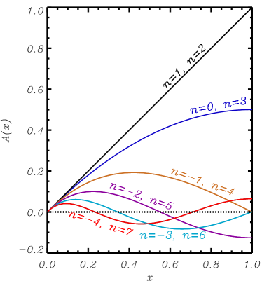
Figure 1.— Potential field solutions $A(x)$ for $n=-4$ (or 7), -3 (or 6), -2 (or 5), -1 (or 4), 0 (or 3), 1 (or 2), 2 (or 1), 3 (or 0), 4 (or -1) and 5 (or -2).

To visualize the magnetic field lines, we use the fact, explained in Section 2 following Equation (24), that the isolines of the magnetic potential $\hat{A}=A(x)/r^{n-2}$ in the poloidal plane are poloidal field lines. Further, equally spaced values of $\hat{A}$ correspond to isolines that contain the same amount of poloidal flux between them (see Sect. 2.9.3 of Priest, 2014). For the diagrams in this section (Figures 2, 3, and 4), however, for better visualization, we are choosing non-equally spaced values of $\hat{A}$ for the isolines. On the other hand, the arrow heads on the field lines in those figures indicate the direction of the magnetic field.

In Figures 2, 3, and 4, we have plotted the poloidal field lines for various cases with $n$ in the ranges $0<n\leq 2$, $n>2$, and $n<0$, respectively. For $n>0$ the origin is a singularity and the field strength declines with distance along each radius. In contrast, for $n<0$ the origin is a null point and the magnetic field strength increases with distance from the origin. For $n=0$ the magnetic field is uniform in space and parallel to the $z$-axis (see Fig. 2a). For $0<n<2$ the field lines bend towards the $z$-axis as $z$ increases (Figure 2, panels b and c). For $n=2$ equation (71) strongly simplifies to just $\ddot{A}=0$. The field lines in this case are straight, radiating in all directions from the origin (Figure 2d) – this solution corresponds to a pure magnetic monopole located at the origin of coordinates.

For $n>2$ the field lines curve away from the $z$-axis as $z$ increases, and form loops, closing down to meet the horizontal axis (Fig. 3c). For $n=3$ the field lines are vertical where they meet the surface $z=0$. For $n=4$ the field lines are loops that start and close at the origin with one lobe in between. For $n=5$ the structure is more complex with one lobe and one magnetic separatrix. In this situation the magnetic field is also vertical at the surface $z=0$. For larger $n$ values more complex structures are obtained such that for $n=6$ there are 2 lobes, for $n=8$ there are 3 lobes, for $n=10$ there are 4 lobes and so on.

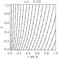
Figure 2.— Potential field solutions, showing the poloidal magnetic field for $n=0,0.5,1$, and $2$.

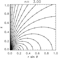
Figure 3.— Potential field solutions, showing the poloidal magnetic field for $n=3,4,5,6,7$, and $8$.

In Figure 4, we have plotted several cases with $n<0$, for which the magnetic field vanishes at the origin. The solutions with integral negative $n$ are particularly simple: they have field distributions on the horizontal plane that are either horizontal or vertical and the solution can easily be extended to the whole space including negative values of $z$. The case $n=-1$ turns out to be a standard 3D null point with the $z$-axis being the spine and the field in the horizontal plane being the fan (Priest & Titov, 1996). For arbitrary negative (but still integer) $n$, the value of $-n$ determines the number of fan surfaces (fan cones, in fact) possessed by the solution: $n=-5$, for instance has five fan surfaces (of which three are apparent in the quadrant shown in Figure 4, bottom right panel). In the general case when $n$ is not an integer, the magnetic field intersects the horizontal axis at an angle different from $0$ or $\pi/2$: for example, the ranges $3<n<4$ or $-2<n<-1$ yield an inclination between $\pi/2$ and $0$, while for $2<n<3$ or $-1<n<0$ the inclination lies between $\pi/2$ and $\pi$.

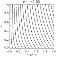
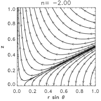
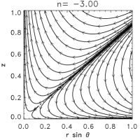
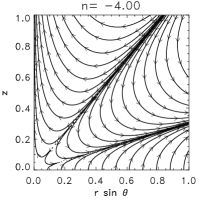
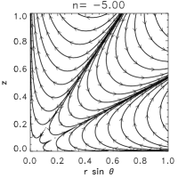
Figure 4.— Potential field solutions, showing the poloidal magnetic field for $n=-0.5,-1,-2,-3,-4$ and $-5$.

Simple trigonometric expressions can be found as solutions for $A$ in Equation (71) when $n$ is a positive or negative integer. Those solutions indicate the number of lobes (for $n>0$) or fan surfaces (for $n<0$) found above, and also justify the fact that the corresponding field lines are either tangential or perpendicular to the equatorial plane. We recall that the solution for $A$ is identical for $n$ and $3-n$. These trigonometric expressions can be found using the relation between the Hypergeometric functions, ${}_{2}F_{1}$ and the associated Legendre polynomials, $P^{1}_{n-2}(1-x)$. When $n=-1$ or $4$, $A=\cos\theta\sin^{2}\theta$, such that $n=4$ gives a single lobe and $n=-1$ gives a first-order null point with one spine and one fan surface. On the other hand $n=-3$ or 6 gives $A=\cos\theta\sin^{2}\theta(3-7\cos^{2}\theta)$, such that $n=6$ has two lobes and $n=-3$ gives a third-order null with two fans (see Fig. 4). Again $n=8$ gives three lobes, while $n=-5$ has three fans, and so on.

4.2. Non-potential Force-Free Field Solutions (${c}_{\phi}\neq 0$)

To obtain solutions for the non-potential force-free case, one must solve Equations (68) and (69) now with $c_{\phi}\neq 0$. We note in passing that the force-free ${\alpha_{ff}}$ coefficient such that $\nabla\times{\vec{B}}={\alpha_{ff}}\,{\vec{B}}$ can be written in our case:

$${\alpha_{ff}}=\pm\,\frac{n-1}{n-2}\,c_{\phi}\;\frac{|A|^{\frac{1}{n-2}}}{r}\;\;=\;\,\pm\,\frac{n-1}{n-2}\frac{|b|^{\frac{1}{n-1}}}{r}\,.$$ (73)

The first expression says that ${\alpha_{ff}}$ is essentially $c_{\phi}$ times a power of the magnetic potential $\hat{A}$ whose isolines coincided with the poloidal field lines: this agrees with the fact that ${\alpha_{ff}}$ must be invariant along each field line. From (73) we also see that the $c_{\phi}$ parameter provides a measure of the field line twist.

Equation (69) is non-linear in $A$, yet it fulfills the following scaling law: given any arbitrary constant $\lambda>0$, if $A=f(x;c_{\phi})$ is a solution, then

$$A=\lambda f(x;c_{\phi}\lambda^{\frac{1}{n-2}})$$ (74)

is also a solution. So, once we have found a solution for a given $c_{\phi}$, we immediately have a whole family of equivalent solutions for all strictly positive values of $c_{\phi}$. Alternatively: imagine you impose constraint $\dot{A}(0)=1$ and find solutions of the equation for all admissible $c_{\phi}$. Then you immediately have solutions for all other values of $\dot{A}(0)$ just by using the scaling law (74). In this sense we will use here again the normalization $\dot{A}(0)=1$ of Section 4.1 without loss of generality. Additionally, as explained earlier, one must impose the boundary condition that $A(0)=0$, for the field to be vertical on the $z$-axis. There exist solutions of Equation (69) only for $n>2$. For $n<2$ it is not possible to find a solution, since $|A|^{\frac{n}{n-2}}$ is singular and cannot be compensated by the other terms on the left-hand side: on the one hand, $A(x\to 0)\to 0$; on the other, the term $x(2-x)\ddot{A}$ behaves as $x^{l-1}$ when $x\to 0$, so it also tends to $0$ since $l\geq 1$ as seen above to make the horizontal field components vanish at the axis. We conclude that $n<2$ is a forbidden region for self-similar force-free field solutions. In particular, there are no solutions with $n<0$.

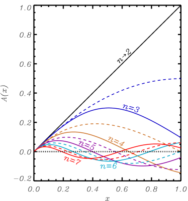
Figure 5.— Force-free solutions $A(x)$ for different values of $n\geq 2$. The solid lines correspond to the force-free field solutions with $c_{\phi}=5$. The dashed lines are the equivalent potential solutions (Sec. 4.1).

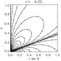
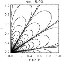
Figure 6.— Force-free field solutions, showing the poloidal magnetic field for $n=3,4,7$ and 8 when $c_{\phi}=5$.

We have solved numerically Equation (69) for $n>2$ with the boundary conditions mentioned above: the result, for the particular case $c_{\phi}=5$, can be seen in Figure 5. To highlight the difference to the potential solutions, the latter have been overplotted as dashed lines. In general the non-potential solutions have their extrema closer to the $x=0$ axis than the potential ones. For example, for $n=4$ the maximum of $A(x)$ is located at $x=0.4$ in the potential case but at $x=0.25$ in the force-free case. Also: the solution crosses the horizontal axis at $x=1$ for the potential case but at $x=0.63$ for the force-free situation. For a sufficiently large $c_{\phi}$ additional extrema and crossing points will appear between $x=0$ and $x=1$ in the force-free solutions when compared with the potential cases. The curve for $n\to 2$ in Figure 5 has been obtained as an asymptotic limit: equation (69) becomes singular in that limit, but the solutions for $A(x)$ tend to the straight line shown for values of $n$ increasingly close to $2$. This limit has been studied by Lynden-Bell & Boily (1994): they find a singularity at a surface $\theta=$const (called sheet discharge by them) which contains purely azimuthal field while in the remaining volume the field is purely radial.

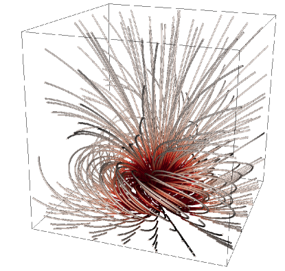
Figure 7.— Three-dimensional plot of the force-free magnetic field lines for $n=3$ and $c_{\phi}=5$. The red color of the lines indicates the intensity of the magnetic field. The darkest red indicate the stronger field intensity and the grey indicates the weaker values.

In Figure 6 the poloidal field lines are plotted for $n>2$. There are important differences compared to the potential situation without twist in Figure 3. For example, the potential field with $n=3$ is perpendicular to the horizontal axis; however, when twist is added the field lines are considerably inclined with respect to the vertical direction. In fact in this situation the field lines are almost closed. In general, the field lines are modified to a large extent at the bottom of the figures with respect to the potential field situation. There is a correspondence between the fans and lobes in both situations for all $n$ shown in the figure.

A balance between the magnetic pressure gradient and poloidal tension non longer holds and so the poloidal field is modified to compensate for the azimuthal magnetic tension. In Figure 7, the three-dimensional field lines for $n=3$ are shown. The magnetic field forms loops starting at the centre and returning to the bottom surface. The magnetic field intensity decreases with distance from the centre of the structure. The field structure has twist that is more pronounced close to the horizontal axis in this particular case. The reason is that $b_{\phi}$ and so the twist depend on $A(x)$ (Equation 68). This function has a maximum close to $x=0.5$ as we see in Figure 5 which corresponds to an angle of approximately 60 degrees with respect to the $z$-axis.

5. Non force-free solutions without poloidal flows ($\Psi=0$)

In this section we consider a more general case in which the Lorentz force is allowed to be non-zero. For the sake of compactness only specific cases are considered that can be analyzed in some detail. We focus on problems without poloidal flow by setting $\Psi=0$ but consider non-zero values of the density $\rho$. Equation (48) is then trivially satisfied. The $\phi$-components of the induction and momentum equations, (49) and (52), become:

$$\left(n+m-1\right)\frac{U}{\rho\,x\,\left(2-x\right)}\,\dot{A}~{}~{}~{}~{}~{}~{}~{}~{}~{}~{}~{}~{}~{}~{}~{}~{}~{}~{}~{}~{}$$

$$\,-\,\frac{d}{dx}\left\{(n-2)\frac{U}{\rho\,x\left(2-x\right)}\,A\right\}\; = 0\;,$$ (75)

$$(n-1)\dot{A}\,b+(2-n)A\,\dot{b}\; = 0\;.$$ (76)

These equations have simple algebraic solutions:

$${|U|\over\rho}\, = \,c_{U}\,\,x\,\left(2-x\right)|A|^{\frac{(m+1)}{(n-2)}}\,,$$ (77)

$$|b| = c_{\phi}\;\;{|A|}^{\frac{n-1}{n-2}}\,,$$ (78)

where the last equation is identical to Equation (68) for the force-free field situation: in the absence of poloidal flows, the $\phi$-component of the Lorentz force must vanish, which is the condition that led to Equations (67) and (68). The integration constants $c_{U}$ and $c_{\phi}$ are positive. The two remaining equations in the system (49)–(52) are the radial and $\theta$ components of the momentum equation, which for $\Psi=0$ simplify to:

$$\frac{U^{2}}{\rho}+2n\,\,p\,x\left(2-x\right)+$$ (79)

$$~{}~{}~{}~{}~{}~{}~{}~{}~{}~{}~{}-\rho gx\left(1-x\right)\left(2-x\right)\,+A\,\mathcal{F}(A,\ddot{A})=0\,,$$

$$\frac{\left(1-x\right)}{x\left(2-x\right)}\frac{U^{2}}{\rho}-\dot{p}\,x\left(2-x\right)+$$ (80)

$$~{}~{}~{}~{}~{}~{}~{}~{}~{}~{}~{}+\rho\,g\,x\,\left(2-x\right)\,-\frac{\dot{A}}{n-2}\mathcal{F}(A,\ddot{A})=0\,,$$

where

$$\mathcal{F}(A,\ddot{A}) \equiv (n-1)\;\hbox{sign}(A)\;c_{\phi}^{2}\;|A|^{n\over n-2}+$$

$$(n-2)^{2}(n-1)\,A\;+\;(n-2)\,x\,(2-x)\ddot{A}\,,$$

and Equation (78) has been used. Additionally, one must keep in mind the constraint discussed above that $m=-1/2$ whenever $g\neq 0$. Equations (79) and (80) represent two equations for the three variables $\rho$, $p$, and $A$. The system can be closed by adding a relation of the kind $p=p(\rho)$, such as, e.g., a polytropic relation $p\propto\rho^{\gamma}$ (discussed in Section 3.2). These two equations are coupled through the $\mathcal{F}$ term, and can be combined to give an instructive form

$$\left[\frac{\dot{A}}{(n-2)A}+\frac{1-x}{x(2-x)}\right]\,\frac{U^{2}}{x\,(2-x)\,\rho}+\left[\frac{2\,n\,p\,\dot{A}}{(n-2)A}-\dot{p}\right]=$$

$$~{}~{}~{}~{}~{}~{}~{}~{}~{}~{}~{}~{}~{}~{}~{}~{}~{}~{}~{}~{}~{}~{}~{}~{}~{}~{}~{}~{}~{}~{}~{}=\rho g\left[\frac{(1-x)\dot{A}}{(n-2)A}-1\right]\,,$$ (82)

which is the fundamental equation for the situation studied in this section, since it illustrates the relations between different parts of the system. Two different possibilities are discussed in the following sections, namely: studying the effects of the gas pressure in the absence of rotation and gravity ($U=0$, $g=0$; Section 5.1); including rotation but disregarding gas pressure (zero-$\beta$ limit) and gravity (Section 5.2). A third possibility exists: disregarding gas pressure (zero-$\beta$ limit) and rotation ($U=0$), but keeping gravity. However, in this case gravity cannot be balanced along the symmetry axis or, in other words, any solution to the equations must have a singularity along the symmetry axis. So no physical solutions can be found in that case.

By analyzing the asymptotic behavior of the different quantities as $x\to 0$ on the basis of the foregoing equations together with the general considerations of Section 3.1 one can obtain algebraic relations limiting the admissible ranges for the exponents $m$, $n$, etc. However, given that we are going to deal with specific solutions which have more restrictive conditions on the exponents, we shall treat the restrictions individually in each subsection.

5.1. Effect of gas pressure

The first case is a natural generalization of the force-free situation considered in Section 4.2. We limit ourselves to the case without rotation and without gravity, $U=0;g=0$. From Equation (82), we obtain

$$p=c_{p}|A|^{\frac{2n}{n-2}}\,,$$ (83)

implying that the isosurfaces of $p$ and $A$ coincide. Since $A(x\to 0)\to 0$, we see that, for the pressure not to become singular toward the axis either $n>2$ or $n\leq 0$. Combining this with (79) one finds

$$x\,(2-x)\,\ddot{A}\,+\,(n-2)\,(n-1)\,A+$$ (84)

$$~{}~{}~{}~{}~{}~{}~{}~{}+\frac{(n-1)}{(n-2)}\;c_{\phi}^{2}\;\hbox{sign}(A)\;|A|^{\frac{n}{n-2}}+$$

$$~{}~{}~{}~{}~{}~{}~{}~{}+\frac{2n}{(n-2)}\;c_{p}\;x\;(2-x)\;\hbox{sign}(A)\;|A|^{\frac{n+2}{n-2}}\quad=\quad 0\,,$$

which generalizes Lynden-Bell & Boily (1994)’s Equation (69) by adding the gas pressure term (last term in the equation). We first study the solutions for the case $n\geq 2$ and compare them with those found in section 4.2. In that section we had had to exclude the negative-$n$ cases since Equation (69) could not be fulfilled near the axis. At the end of this subsection we explore whether the extra term in Equation (84) can modify the negative result of the earlier section.

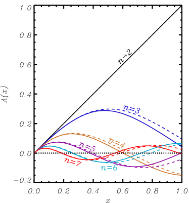
Figure 8.— Solid curves: solutions $A(x)$ for the case with gas pressure (Sec. 5.1) for different values of $n\geq 2$ with $c_{\phi}=5$ and $c_{p}=50$. The dashed lines are the corresponding force-free solutions (Sec. 4.2).

For $n>2$ we numerically integrate this equation to obtain $A(x)$ with the boundary condition $A(0)=0$; also, for specificity, we arbitrarily choose $\dot{A}(0)=1$ (but could use other values if we wanted to explore the parameter space). In Figure 8 several solutions are plotted for $A$ for $n\geq 2$ alongside the force-free solutions (dashed) already studied ; in Figure 9 the actual field lines are shown in the poloidal plane: in both figures the force-free solution is drawn solid and the non-force-free one dashed. We see that, at least for $n=3$ and $4$, the field lines close in on themselves nearer the central axis than in the force-free case. Checking with Figure 5, we see that, mathematically, this is due to the fact that the point $\dot{A}=0$ is reached for smaller $x$ in the potential than in the force-free case: since the field lines are isolines of $\hat{A}=A(x)/r^{n-2}$ (as follows from Equation 34), along each field line the points where $\dot{r}=0$ and $\dot{A}=0$ must coincide: the turning point of the field line (where $\dot{r}=0$) occurs at smaller $x$ for the non force-free case. The physical reason for this behaviour, on the other hand, can be seen as follows: the pressure gradient must be zero along each individual field line, since there is no Lorentz force component in that direction to compensate for it. So, looking at the plane drawn in Figure 9, the pressure gradient is parallel to the gradient of $\hat{A}$. The value of $\hat{A}$, in fact, decreases when jumping outward from one field line to the next, and so must the pressure. Hence the pressure gradient force points outward, and the Lorentz force must be reinforced to compensate for it: the extra curvature of the poloidal field lines helps in doing that; by studying the Lorentz force term ${\cal F}(A,\ddot{A})$ in Equations (79)–(5), one can conclude that both the azimuthal and poloidal field components help to reinforce the Lorentz force in this case. From the Figure we also see that, for these $n\geq 2$ solutions, the influence of the pressure is most marked at large $x$, i.e., large $\theta$, whereas it is unimportant near the axis.

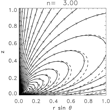
Figure 9.— Poloidal magnetic field for $n=3$, and $4$ for the situation with gas pressure with $c_{\phi}=5$ and $c_{p}=50$. In order to understand the role of the gas pressure in the equilibrium we have also plotted the force-free field as dashed lines.

We finish by considering the $n<0$ solutions. The reason why there were no such solutions in the force-free case of Section 4.2 was that the magnetic pressure term $x(2-x)\ddot{A}$ could not be balanced by any other term in Equation 69. Now we see that the new extra term, the gas pressure term, is in no position to compensate for it, either, so the negative-$n$ solutions must be excluded also here. The solutions in this section therefore have closed field lines and no open field lines are allowed. Thus, no collimated structures appear with the new gas pressure term.

5.2. Effect of rotation

To explore the effects of rotation, we here go to the zero-$\beta$ (i.e., no gas-pressure) limit without gravity; from (82) we then see that

$$\frac{\dot{A}}{A}=(2-n)\frac{1-x}{x(2-x)}\,,$$ (85)

which is easily integrable to

$$A(x)=c_{A}\left[x(2-x)\right]^{\frac{2-n}{2}}\,,$$ (86)

with $c_{A}$ an integration constant that coincides with $A(1)$. Given the definition of $x$, $A(x)$ is therefore monotonic and simply proportional to $\sin^{2-n}\theta$. We are free to select its global sign, and in the following assume $A(x)>0$. From (86), for $A$ to vanish at the axis, $(2-n)/2\geq~{}1$, i.e., $n\leq~{}0$. As we shall see, $n=0$ does not satisfy the asymptotic conditions for $b$ at the axis and so the allowed values are $n<0$ : it is interesting to see that in this case solutions with a collimated structure are found as in the case of a potential field (Sect. 4.1).

In Figure 10 several normalized solutions $A(x)/c_{A}$ are plotted for different values of $n$. For all the allowed $n$ values the derivative of $A$ at the origin is zero. For $n=-0.1$ the function rapidly grows very close to the origin. For smaller values of $n$ the growth is less pronounced, and for $n=-20$ the function is close to zero for a large portion of the domain.

Figure 10.— Pure rotation with no gravity and low temperature, showing the lowest-order magnetic potential $A(x)/c_{A}$ for several values of $n<0$.

From Equations (77) to (5) we find

$$\rho(x)=c_{\rho}\,\left[x\,(2-x)\right]^{m-n}\,,$$ (87)

where

$$c_{\rho}\equiv\frac{(1-n)c_{A}^{\frac{2}{n-2}}-n\,(n-2)^{2}\,c_{\phi}^{-2}}{c_{U}^{2}\,c_{\phi}^{-2}\,c_{A}^{\frac{2(3+m-n)}{n-2}}}\,.$$ (88)

Combining Equations (77), (78), (86), and (87) we obtain

$$U(x) = c_{U}\,c_{\rho}\,c_{A}^{\frac{1+m}{n-2}}\left[x(2-x)\right]^{\frac{1}{2}(m-2n+1)}\,,$$ (89)

$$b(x) = c_{\phi}\,c_{A}^{\frac{n-1}{n-2}}[x(2-x)]^{\frac{(1-n)}{2}}\,.$$ (90)

The exponents of the square bracket terms in (87), (89) and (90) directly give the asymptotic behavior of $\rho(x)$, $U(x)$ and $b(x)$ when $x\to~{}0$. In Section 3.1 we had given the symbols ${\sigma}$, $\nu$ and $\omega$, respectively, for those exponents and seen that they must fulfill relations (59) – (60), additionally to the condition ${\sigma}\geq 0$ for $\rho$ not to be singular at the axis. Putting all that together we conclude that $n\leq m<0$. In Figure 11 the region of allowed $m$ and $n$ is plotted as a shaded area. For $m$ and $n$ on the line $m-n=0$ (thick line), the density $\rho(x)$ is independent of $x$ according to Equation (87).

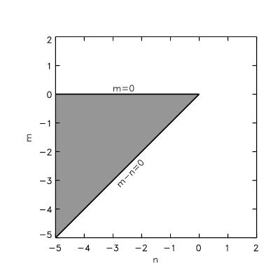
Figure 11.— Allowed values of $m$ and $n$ for pure rotation and a zero-$\beta$ plasma given by the axisymmetric conditions. In the white area at least one of the conditions is not fulfilled. The shaded area gives the allowed values for solutions of Equation (86). The solid thick lines are plotted to show that these values are included in the region of validity.

From Equation (88) we see that the four coefficients $c_{\rho},c_{A},c_{U}$, and $c_{\phi}$ are related. This implies that we have freedom to fix three of the four coefficients and the remaining one is set by this relation. For example, fixing the magnetic structure (with $c_{A}$ and $c_{\phi}$) and a given rotation velocity ($c_{U}$), the density ($c_{\rho}$) accommodates accordingly. Similarly, for a given magnetic field structure and density the plasma will rotate with a given profile. For the allowed values of $n<0$ the coefficient $c_{\rho}$ is always positive as expected.

The structure of the magnetic field in this situation is quite simple. Calling ${\varpi}$ the cylindrical radius, i.e., ${\varpi}=r\,\sin\theta=r\sqrt{x(2-x)}$, and ${B_{\varpi}}$ the field component in that direction, ${B_{\varpi}}=B_{r}\,\sin\theta+B_{\theta}\,\cos\theta$, we see that for all allowed values of $n$, the poloidal field is everywhere aligned with the $z$-axis:

$${B_{\varpi}} = 0\,,$$ (91)

$$B_{z} = B_{r}\,\cos\theta\,-\,B_{\theta}\sin\theta\,\;=\;\,(2-n)\,c_{A}\,{\varpi}^{-n}\;.$$ (92)

To obtain that result one must use Equations (44), (45) and (86). When written out in their full dependence with $r$ and $\theta$, the other magnitudes $B_{\phi}$, $\rho$, and $v_{\phi}$ can also be seen to depend ${\varpi}$ only, as follows:

$$B_{\phi}(r,\theta) = c_{\phi}\,c_{A}^{\frac{n-1}{n-2}}{\varpi}^{-n}\,,$$ (93)

$$\rho(r,\theta) = c_{\rho}\,{\varpi}^{2(m-n)}\,,$$ (94)

$$v_{\phi}(r,\theta) = c_{U}\,c_{A}^{\frac{1+m}{n-2}}\,{\varpi}^{-m}\,.$$ (95)

The system therefore has cylindrical symmetry; the index $n$ can take any negative value, indicating that the magnetic field always increases with the distance from the rotation axis. The index $m$ is constrained by the condition $0>m\geq n$ (see Fig. 11). Thus, the rotation velocity $v_{\phi}$ can increase ($m<0$) with distance from the rotation axis but never faster than the magnetic field. The density [Equation (94)] depends on the $m-n$ index, which is always positive (Fig. 11). For $m-n>0$ the density vanishes at the rotation axis and increases with distance from this axis. The profile of $\rho$ complements the constraint on $v_{\phi}$ in that $\rho v_{\phi}^{2}$ has the same dependence on ${\varpi}$ as $B_{\phi}^{2}$, expected to maintain dynamical equilibrium.

Figure 12 shows the three-dimensional magnetic field lines. The cylindrical symmetry of the system is apparent. In the cases shown the magnetic field vanishes at the rotation axis: for $n=-0.1$ (top panel) the magnetic field is more uniform than in the case of $n=-2$ (bottom panel), as follows from the simple power-laws of (92) and (93).

In general, the field line inclination is given by the ratio of $B_{\phi}/B_{z}$, which, after using Equations (92) and (93), becomes

$$\frac{B_{\phi}}{B_{z}}=\frac{1}{2-n}\,c_{\phi}\,c_{A}^{\frac{1}{n-2}}\,,$$ (96)

and so is independent of position.

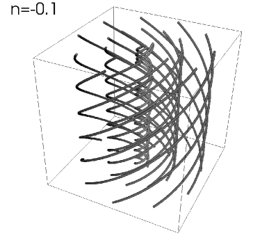
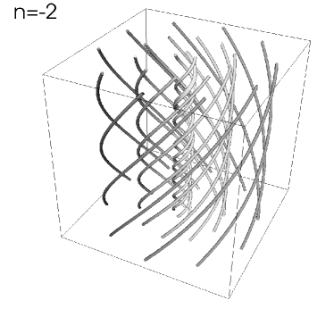
Figure 12.— Pure rotation in the zero-$\beta$ limit and with no gravity, showing the field lines for the magnetic field of Equations (86) and (90). The color code indicates the strength of the magnetic field from white to black. The magnetic field for $n=-0.1$ and $n=-2$ solutions are shown in the top and bottom panel, respectively. In both cases $c_{\phi}=2$ and $c_{A}=2$.

The uniformity of the ratio $B_{\phi}/B_{z}$ matches the visual impression in Figure 12. The maximum inclination is reached for $n=0$ and decreases when $n$ decreases for constant $c_{\phi}$ and $c_{A}$.

The physical quantities in the foregoing solutions ($B,\rho,v_{\phi}$) all increase with the cylindrical radius ${\varpi}$. Hence their application must necessarily be limited to a finite region of space, i.e., beyond a given radius they should be matched with an external solution via adequate boundary conditions. Wherever such matching can be carried out successfully, these solutions could provide useful insights into the nature of rotating MHD structures.

6. Discussion and Conclusions

In this work we have set up models for MHD structures that are axisymmetric and steady state. We have sought self-similar solutions of the form $f(\theta)/r^{n}$ with each variable having a different function $f(\theta)$ and power, $n$. We have proceeded from the simplest situation to ones of increasing complexity.

The first system we consider is a potential field , so necessarily with no electric current and no magnetic twist. We have found analytical solutions for different values of $n$. For $n>0$ the origin of coordinates is a source of magnetic field and its strength declines with distance. In contrast, for $n<0$ the origin is a null point and the magnetic field strength increases. For $n=0$ the magnetic field is uniform in space and parallel to the $z$-axis. For $0<n<2$ the field lines curve towards the the $z$-axis and for $n=2$ the field lines are straight, but radiate in all directions from the origin. For $n>2$ they curve away from the $z$-axis and form loops, closing back down to meet the horizontal axis. One of the most sets of interesting solutions is the set with $n<0$. Here the magnetic field at the origin vanishes and so there is a null point there with no closed lines. For $n=-0.5$ the field lines are curved with respect to the vertical field forming a collimated magnetic structure. For $n=-1$ the magnetic field is identical to a first-order null point with a typical X shape at the origin. For $n=-2$, the solution has a fan in the domain and for $n<-2$ the complexity increases with an increasing number of fans. This simple solution reveals that it is necessary to have $n$ negative to form a collimated structure around the axis. The collimated structure consists of open field lines that accumulate around the axis.

The second system we consider is force-free and includes twist. There exist solutions here only for $n\geq 2$ where the field forms loops starting at the centre returning again to the bottom surface as in the potential situation. However, the presence of the azimuthal component twists the loops around the axis. The case with $n\geq 2$ is similar to the case studied by Lynden-Bell & Boily (1994) but with different boundary conditions. In this case, the $n<0$ solutions are forbidden and no collimated magnetic structures appear: the extra force associated with the new azimuthal term cannot be balanced by the poloidal magnetic pressure and tension at the axis.

We then increased the complexity of the system by considering a more general situation, namely non-force free cases but still with no poloidal flows. This allows us to study structures with non-vanishing gas pressure, rotation, or gravity. The first case is a system with magnetic field and gas pressure but without rotation and gravity. This extends Lynden-Bell&Boily’s force-free solutions by adding gas pressure. The solutions have field lines that are more highly curved than in the force-free solutions: the extra pressure gradient must be balanced by the magnetic force. Also, the gas pressure is more important close to the horizontal axis. The allowed solutions have $n\geq 2$ indicating that the extra pressure cannot balance the magnetic pressure at the axis when $n<2$. As in the non-potential force-free situation the resulting structure is not collimated around the axis.

For rotating zero-$\beta$ plasma structures we find analytical solutions for the magnetic field, rotational velocity, and density fields. They all possess a cylindrical geometry and depend solely on distance from the rotation axis but they exist only for $n<0$. The magnetic field has twist that depends on the index $n$. The density and rotation velocity increase with the distance from the centre. The new velocity term introduces a centrifugal force, that contributes to the balance of the Lorentz force associated with the poloidal and azimuthal components of the magnetic field. In fact, the poloidal field consists of straight field lines indicating that the poloidal tension vanishes, and the centrifugal force balances the inward magnetic pressure and azimuthal tension forces.

Summarizing, in this paper we have formulated general equations for the steady-state ideal MHD problem assuming axisymmetry and self-similarity and including flows, gas pressure and gravity. Also, a number of solutions have been calculated including potential, force-free and non-force free ones. The results can be used as a starting point for future developements, such as, for example, including poloidal flows in the solutions. In Luna et al. (2015) we showed that the combination of magnetic twist and poloidal flow can induce a force along the axis of the structure. This is an interesting scenario for producing jets and supporting the cool plasma against gravity in the solar corona.

References

- Abramowitz & Stegun (1972) Abramowitz, M., & Stegun, I. A. 1972, Handbook of Mathematical Functions, ed. Abramowitz, M. & Stegun, I. A.
- Blundell & Hirst (2011) Blundell, K. M., & Hirst, P. 2011, ApJ, 735, L7
- Boettcher et al. (2012) Boettcher, M., Harris, D. E., & Krawczynski, H. 2012, Relativistic Jets from Active Galactic Nuclei
- Bonet et al. (2008) Bonet, J. A., Márquez, I., Sánchez Almeida, J., Cabello, I., & Domingo, V. 2008, ApJ, 687, L131
- Bonet et al. (2010) Bonet, J. A., Márquez, I., Sánchez Almeida, J., et al. 2010, ApJ, 723, L139
- Canfield et al. (1996) Canfield, R. C., Reardon, K. P., Leka, K. D., et al. 1996, ApJ, 464, 1016
- Cattaneo et al. (2003) Cattaneo, F., Emonet, T., & Weiss, N. O. 2003, ApJ, 588, 1183
- De Pontieu et al. (2012) De Pontieu, B., Carlsson, M., Rouppe van der Voort, L., et al. 2012, ApJ, 752, L12
- De Pontieu et al. (2014) De Pontieu, B., Rouppe van der Voort, L., McIntosh, S. W., et al. 2014, Science, 346, 1255732
- Fabian et al. (2014) Fabian, A. C., Walker, S. A., Celotti, A., et al. 2014, MNRAS, 442, L81
- Ferrari et al. (2011) Ferrari, A., Mignone, A., & Campigotto, M. 2011, in IAU Symposium, Vol. 274, Advances in Plasma Astrophysics, ed. A. Bonanno, E. de Gouveia Dal Pino, & A. G. Kosovichev, 410–415
- Gracia et al. (2009) Gracia, J., de Colle, F., & Downes, T., eds. 2009, Lecture Notes in Physics, Berlin Springer Verlag, Vol. 791, Jets From Young Stars V
- Gu et al. (1994) Gu, X. M., Lin, J., Li, K. J., et al. 1994, A&A, 282, 240
- Jibben & Canfield (2004) Jibben, P., & Canfield, R. C. 2004, ApJ, 610, 1129
- Levens et al. (2015) Levens, P. J., Labrosse, N., Fletcher, L., & Schmieder, B. 2015, A&A, 582, A27
- Lovelace et al. (1986) Lovelace, R. V. E., Mehanian, C., Mobarry, C. M., & Sulkanen, M. E. 1986, ApJS, 62, 1
- Luna et al. (2015) Luna, M., Moreno-Insertis, F., & Priest, E. 2015, ApJ, 808, L23
- Lynden-Bell & Boily (1994) Lynden-Bell, D., & Boily, C. 1994, MNRAS, 267, 146
- Mestel (1961) Mestel, L. 1961, Mon. Not. Roy. Astron. Soc., 122, 473
- Nordlund et al. (2009) Nordlund, Å., Stein, R. F., & Asplund, M. 2009, Liv. Rev. in Solar Phys., 6, 1
- Orozco Suárez et al. (2012) Orozco Suárez, D., Asensio Ramos, A., & Trujillo Bueno, J. 2012, ApJ, 761, L25
- Priest (2014) Priest, E. 2014, Magnetohydrodynamics of the Sun (Cambridge University Press)
- Priest & Titov (1996) Priest, E. R., & Titov, V. S. 1996, Philosophical Transactions of the Royal Society A: Mathematical, 354, 2951
- Requerey et al. (2017) Requerey, I. S., Del Toro Iniesta, J. C., Rubio, L. R. B., et al. 2017, ApJS, 229, 14
- Smith (2012) Smith, M. D. 2012, Astrophysical Jets and Beams
- Srivastava et al. (2017) Srivastava, A. K., Shetye, J., Murawski, K., et al. 2017, Scientific Reports, 7, 43147
- Steiner et al. (2010) Steiner, O., Franz, M., Bello González, N., et al. 2010, ApJ, 723, L180
- Su et al. (2014) Su, Y., Gömöry, P., Veronig, A., et al. 2014, ApJ, L2
- Su et al. (2012) Su, Y., Wang, T., Veronig, A., Temmer, M., & Gan, W. 2012, ApJ., 756, L41
- Tsinganos et al. (2006) Tsinganos, K., Meliani, Z., Sauty, C., Vlahakis, N., & Trussoni, E. 2006, in American Institute of Physics Conference Series, Vol. 848, Recent Advances in Astronomy and Astrophysics, ed. N. Solomos, 560–569
- Tsinganos et al. (2009) Tsinganos, K., Ray, T., & Stute, M. 2009, Astrophysics and Space Science Proceedings, 13
- Tsinganos & Sauty (1992) Tsinganos, K., & Sauty, C. 1992, A&A, 257, 790
- Tsinganos (2007) Tsinganos, K. C. 2007, in Lecture Notes in Physics, Berlin Springer Verlag, Vol. 723, Lecture Notes in Physics, Berlin Springer Verlag, ed. J. Ferreira, C. Dougados, & E. Whelan, 117–
- Tsinganos (2010) Tsinganos, K. C. 2010, Mem. della Soc. Astron. Ital., 15, 102
- Wedemeyer-Böhm & Rouppe van der Voort (2009) Wedemeyer-Böhm, S., & Rouppe van der Voort, L. 2009, A&A, 507, L9
- Wedemeyer-Böhm et al. (2012) Wedemeyer-Böhm, S., Scullion, E., Steiner, O., et al. 2012, Nature, 486, 505