Singular perturbation analysis of a regularized MEMS model

Abstract

Micro-Electro Mechanical Systems (MEMS) are defined as very small structures that combine electrical and mechanical components on a common substrate. Here, the electrostatic-elastic case is considered, where an elastic membrane is allowed to deflect above a ground plate under the action of an electric potential, whose strength is proportional to a parameter $\lambda$. Such devices are commonly described by a parabolic partial differential equation that contains a singular nonlinear source term. The singularity in that term corresponds to the so-called “touchdown” phenomenon, where the membrane establishes contact with the ground plate. Touchdown is known to imply the non-existence of steady-state solutions and blow-up of solutions in finite time.

We study a recently proposed extension of that canonical model, where such singularities are avoided due to the introduction of a regularizing term involving a small “regularization” parameter $\varepsilon$. Methods from dynamical systems and geometric singular perturbation theory, in particular the desingularization technique known as “blow-up”, allow for a precise description of steady-state solutions of the regularized model, as well as for a detailed resolution of the resulting bifurcation diagram. The interplay between the two principal model parameters $\varepsilon$ and $\lambda$ is emphasized; in particular, the focus is on the singular limit as both parameters tend to zero.

34B16, 34C23, 34E05, 34E15, 34L30, 35K67, 74G10

1 Introduction

Micro-Electro Mechanical Systems (MEMS) are very small structures that combine electrical and mechanical components on a common substrate to perform various tasks. In particular, electrostatic-elastic devices have found important applications in drug delivery [30], micro pumps [9], optics [1], and micro-scale actuators [31]. In these devices, an elastic membrane is allowed to deflect above a ground plate under the action of an electric potential $V$, where the distance between plate and membrane is typically much smaller than their diameter; see Fig. 1. When a critical voltage threshold $V^{\ast}$ (“pull-in voltage”) is reached, a phenomenon called touchdown or snap-through can occur, i.e., the membrane touches the ground plate, which may cause a short circuit.

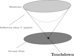
Figure 1: Schematic representation of an electrostatic-elastic MEMS device. The elastic membrane deflects towards the ground plate when an electric potential $V$ is applied (dashed curve). If $V$ exceeds a critical value $V^{*}$ (the so-called “pull-in voltage”), the membrane touches the ground plate, causing touchdown (dotted line).

The physical forces acting between the elastic components of the device – which can, e.g., be of Casimir or Van der Waals type – may lead to stiction, which causes complications in reverting the process in order to return to the original state. In the canonical mathematical models proposed in the literature [8, 18, 24, 25], such systems are described by partial differential equations involving the Laplacian or the bi-Laplacian and a singular source term. The touchdown phenomenon leads to non-existence of steady states, or blow-up of solutions in finite time, or both. Hence, no information on post-touchdown configurations can be captured by these models.

Recently, an extension of the canonical model has been proposed, where the introduction of a potential mimicking the effect of a thin insulating layer above the ground plate prevents physical contact between the elastic membrane and the substrate [20]. Mathematically, a nonlinear source term that depends on a small “regularization” parameter $\varepsilon$ is added to the partial differential equation. The resulting regularized models have been studied in relevant work by Lindsay et al.; see e.g. [20, 22] for the membrane case, while the case where the elastic structure is modelled as a beam is discussed in [19, 20, 22]. In one spatial dimension, the governing equations are given by

(1) $$\begin{split}u_{t}&=u_{xx}-\frac{\lambda}{(1+u)^{2}}+\frac{\lambda\varepsilon^{m-2}}{(1+u)^{m}}\\ &\quad\text{for }x\in[-1,1],\text{ with }u=0\text{ when }x=\mp 1\quad(\text{membrane})\\ \end{split}$$

and

(2) $$\begin{split}u_{t}&=-u_{xxxx}-\frac{\lambda}{(1+u)^{2}}+\frac{\lambda\varepsilon^{m-2}}{(1+u)^{m}}\\ &\quad\text{for }x\in[-1,1],\text{ with }u=\partial_{n}u=0\text{ when }x=\mp 1\quad(\text{beam}),\end{split}$$

respectively. Physically speaking, the variable $u$ denotes the (dimensionless) deflection of the surface, while the parameter $\lambda$ is proportional to the square of the applied voltage $V$. The regularizing term $\lambda\varepsilon^{m-2}(1+u)^{-m}$ with $\varepsilon>0$ and $m>2$, as introduced in [20], accounts for various physical effects that are of particular relevance in the vicinity of the ground plate, i.e., at $u=-1$; that term induces a potential which simulates the effect of an insulating layer whose non-dimensional width is proportional to $\varepsilon$. In the following, we will consider $m=4$, which corresponds to a Casimir effect; alternative choices describe other physical phenomena and can be studied in a similar fashion.

Here, we focus on steady-state solutions of the Laplacian case corresponding to a membrane; see LABEL:LiLap:

(3) $$u_{xx}=\frac{\lambda}{(1+u)^{2}}\bigg{[}1-\frac{\varepsilon^{2}}{(1+u)^{2}}\bigg{]}\qquad\text{ for }x\in[-1,1],\text{ with }u=0\text{ when }x=\mp 1.$$

For literature on the bi-Laplacian case, Equation 2, we refer to [20, 21, 22].

Remark 1.1.

Due to the symmetry of the boundary value problem Eq. 3 under the transformation $x\mapsto-x$, all solutions thereof must be even; the proof is straightforward, and is omitted here.

Before addressing the novel features of the regularized model which are the focus of the present article, we briefly summarize the main properties of the non-regularized case corresponding to $\varepsilon=0$ in Eq. 3, which are well understood [24, 25]. The numerically computed bifurcation diagram associated to Eq. 3 for $\varepsilon=0$ is shown in Fig. 2; it contains two branches of steady-state solutions, where the lower branch is stable and the upper one is unstable. The upper branch limits on the $\|u\|_{2}^{2}$-axis in the point $B=\left(0,\frac{2}{3}\right)$, which plays a crucial role in the bifurcation diagram of the regularized problem. The two branches are separated by a fold point that is located at $\lambda=\lambda^{\ast}$. For $\lambda>\lambda^{\ast}$, steady-state solutions of LABEL:LiLap cease to exist, with the transient dynamics leading to a blow-up in finite time. Sample solutions along the two branches are plotted in Fig. 2; in addition, the piecewise linear singular solution corresponding to the point $B$ is shown. That singular solution undergoes touchdown at $x=0$.

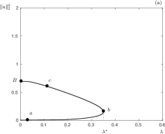
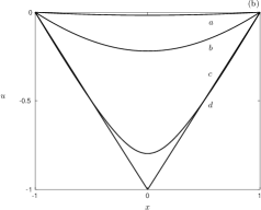
Figure 2: (a) Bifurcation diagram of the membrane model, Equation 3, for $\varepsilon=0$. The lower and upper branches consist of stable and unstable steady-state solutions, respectively. The solution labeled $d$ corresponds to the point $B$ and represents the singular solution for $\lambda=0$. (b) Corresponding solutions in $(x,u)$-space.

The inclusion of the $\varepsilon$-dependent regularizing term, where $0<\varepsilon\ll 1$, considerably alters the structure of the bifurcation diagram in Fig. 2. The principal new feature is the emergence of a third branch of stable steady-state solutions, resulting in the $S$-shaped curve shown in Fig. 3; that diagram was established numerically and via matched asymptotics in [20]. In addition to the fact that the fold point at $\lambda^{\ast}$ now depends on $\varepsilon$, there exists another fold point at $\lambda_{\ast}$ – which is also $\varepsilon$-dependent – such that, for $\lambda_{\ast}<\lambda<\lambda^{\ast}$, there are three branches of steady states, the middle one of which is unstable. Solutions on that newly emergent branch are in fact bounded below by $u=-1+\varepsilon$. With increasing $\lambda$, solutions exhibit a growing “flat” portion close to $u=-1+\varepsilon$; cf. the solution labeled $d$ in Fig. 3. For $\lambda<\lambda_{\ast}$ and $\lambda>\lambda^{\ast}$, there exists a unique stable steady state; in particular, and in contrast to the non-regularized case, numerical simulations indicate that a stable steady state exists for every value of $\lambda>0$.

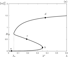
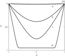
Figure 3: (a) Numerically computed bifurcation diagram of the one-dimensional membrane model, Equation 3, for $\varepsilon=0.05$. The gray circle indicates the point $B=\left(0,\frac{2}{3}\right)$. (b) Corresponding solutions in $(x,u)$-space.

For very small values of $\varepsilon$, the bifurcation diagram in Fig. 3 is difficult to resolve, even numerically. These difficulties are particularly prominent in the vicinity of the upper branch and the fold point at $\lambda_{\ast}(\varepsilon)$; see, e.g., Equation 4 and Remark 4.32 for details. The highly singular nature of the bifurcation diagram in Fig. 3, as well as the influence of the regularization parameter $\varepsilon$ on the structure thereof, are the principal features of interest to us here.
In the present work, we will give a detailed geometric analysis of Equation 3 for small values of $\varepsilon$; in particular, we will prove that the (numerically computed) bifurcation diagram, as shown in Fig. 3, is correct. Moreover, we will explain the underlying structure of that diagram. In summary, our main result can be expressed as follows:

Theorem 1.2.

For $\varepsilon\in(0,\varepsilon_{0})$, with $\varepsilon_{0}>0$ sufficiently small, and $\lambda\in[0,\Lambda]$, with $\Lambda=\mathcal{O}(1)$ positive and fixed, the bifurcation diagram for the boundary value problem Eq. 3 has the following properties:

• In the $(\lambda,\|u\|_{2}^{2})$-plane, the set of solutions to Eq. 3 corresponds to an $S$-shaped curve emanating from the origin. The curve consists of three branches – lower, middle, and upper – that are separated by two fold points which are located at $\lambda=\lambda_{\ast}(\varepsilon)$ and $\lambda=\lambda^{\ast}(\varepsilon)$. Specifically, there exists one steady-state solution to Eq. 3 for $\lambda<\lambda_{\ast}(\varepsilon)$ and $\lambda>\lambda^{\ast}(\varepsilon)$, while for $\lambda_{\ast}(\varepsilon)<\lambda<\lambda^{\ast}(\varepsilon)$, there exist three steady-state solutions.

• Along the lower and upper branches in Fig. 3, $\|u\|_{2}^{2}$ is a strictly increasing function of $\lambda$, whereas $\|u\|_{2}^{2}$ is a decreasing function of $\lambda$ along the middle branch.

• The function $\lambda_{\ast}(\varepsilon)$ is $C^{1}$ in $\varepsilon$ and smooth as a function of $(\varepsilon,\ln\varepsilon)$, and admits the expansion

  $$\lambda_{\ast}(\varepsilon)=\frac{3}{4}\varepsilon-\bigg{(}\sqrt{\frac{3}{2}}+\frac{9}{8}\bigg{)}\varepsilon^{2}\ln\varepsilon+\mathcal{O}(\varepsilon^{2}).$$

  Moreover, $\lambda^{\ast}(\varepsilon)$ is smooth in $\varepsilon$ and admits the expansion

  $$\lambda^{\ast}(\varepsilon)=\lambda_{0}^{\ast}+\lambda_{1}^{\ast}\varepsilon^{2}+\mathcal{O}(\varepsilon^{4}),$$

  with appropriately chosen coefficients $\lambda_{0}^{\ast}$ and $\lambda_{1}^{\ast}$.

• Outside of a fixed neighborhood of the point $B$, the lower and middle branches in Fig. 3 are smooth perturbations of the non-regularized bifurcation curve illustrated in Fig. 2, while the upper branch has the following expansion:

  (4) $$\|u\|_{2}^{2}=2\bigg{(}1-\frac{\sqrt{3}}{3}\sqrt{\frac{\varepsilon}{\lambda}}-2\varepsilon+\mathcal{O}(\varepsilon^{\frac{3}{2}}\ln\varepsilon)\bigg{)}.$$

The detailed asymptotic resolution of the bifurcation diagram associated to the boundary value problem Eq. 3, carried out in the proof of Theorem 1.2, is accomplished through separate investigation of three distinct, yet overlapping, regions in the diagram, both in the singular limit of $\varepsilon=0$ and for $\varepsilon$ positive and sufficiently small. To that end, we first reformulate Eq. 3 in a dynamical systems framework; then, identification of two principal parameters in the resulting equations yields a two-parameter singular perturbation problem. Careful asymptotic analysis of that problem will allow us to identify the corresponding limiting solutions, and to show how the third branch in the diagram found for non-zero $\varepsilon$ emerges from the singular limit of $\varepsilon=0$. On that basis, we will prove the existence and uniqueness of solutions close to these limiting solutions. While the three regions in the diagram share some common features, they need to be investigated separately for the structure of the diagram to be fully resolved.

Our analysis is based on a variety of dynamical systems techniques and, principally, on geometric singular perturbation theory [7, 10, 15] and the blow-up method, or “geometric desingularization” [3, 6, 13]. In particular, a combination of these techniques will allow us to perform a detailed study of the saddle-node bifurcation at the fold point at $\lambda_{\ast}$, and to obtain an asymptotic expansion (in $\varepsilon$) for $\lambda_{\ast}(\varepsilon)$. While such an expansion has been derived by Lindsay via the method of matched asymptotic expansions [20], cf. Figure 12 therein, as well as our Fig. 3, the leading-order coefficients in that expansion are calculated explicitly here. In the process, it is shown that the occurrence of logarithmic switchback terms in the steady-state asymptotics for Equation 3, which has also been observed via asymptotic matching in [20], is due to a resonance phenomenon in one of the coordinate charts after blow-up [26, 27, 28, 29]; cf. Section 4.1.5.

Without loss of generality, we fix $\Lambda=1$ in Theorem 1.2. The proof of Theorem 1.2 follows from a combination of Propositions 4.5, 4.23, and 4.28 below; each of these pertains to one of the three above-mentioned regions in the bifurcation diagram.

The article is structured as follows: in Section 2, we reformulate the boundary value problem Eq. 3 as a dynamical system. In Section 3, we introduce the principal blow-up transformation on which our analysis of the dynamics of Eq. 3 close to touchdown is based. In Section 4, we describe in detail the structure of the bifurcation diagram in Fig. 3 by investigating separately three main regions therein, as illustrated in Fig. 9 below. Finally, in Section 5, we discuss our findings, and we present an outlook to future research.

2 Dynamical Systems Formulation

For our analysis, we reformulate Equation 3 as a boundary value problem for a corresponding first-order system by introducing the new variable $w=u^{\prime}$; here, it is useful to keep in mind that $w$ represents the slope of the solution $u$ to Equation 3. Moreover, we append the trivial dynamics of both the spatial variable $x$, which we relabel as $\xi$, and the regularizing parameter $\varepsilon$, to the resulting system:

(5a) $$u^{\prime} =w,$$

(5b) $$w^{\prime} =\frac{\lambda}{(1+u)^{2}}\bigg{[}1-\frac{\varepsilon^{2}}{(1+u)^{2}}\bigg{]},$$

(5c) $$\xi^{\prime} =1,$$

(5d) $$\varepsilon^{\prime} =0;$$

here, the prime denotes differentiation with respect to $x$. Next, we multiply the right-hand sides in Equation 5 with a factor of $(1+u)^{4}$, which allows us to desingularize the flow near the touchdown singularity at $u=-1$. Finally, we define a shift in $u$ via

(6) $$\tilde{u}=1+u,$$

which translates that singularity to $\tilde{u}=0$.

Omitting the tilde and denoting differentiation with respect to the new independent variable by a prime, as before, we obtain the system

(7a) $$u^{\prime} =u^{4}w,$$

(7b) $$w^{\prime} =\lambda(u^{2}-\varepsilon^{2}),$$

(7c) $$\xi^{\prime} =u^{4},$$

(7d) $$\varepsilon^{\prime} =0$$

in $(u,w,\xi,\varepsilon)$-space, with parameter $\lambda$ and subject to the boundary conditions

(8) $$u=1\qquad\text{for }\xi=\mp 1.$$

Since $\varepsilon$ is small, it seems natural to attempt a perturbative construction of solutions to the boundary value problem {Eq. 7,Eq. 8}, which turns out to be non-trivial in spite of the apparent simplicity of the governing equations. For $\varepsilon=0$, Equation 7 can be solved explicitly and admits degenerate equilibria at $u=0$, which corresponds to the touchdown singularity at $u=-1$ in the original model, Equation 3. We denote the resulting manifold of equilibria for Eq. 7 as

(9) $$\SS^{0}=\big{\{}(0,w,\xi,0)\,\big{|}\,w\in\mathbb{R},\ \xi\in\mathbb{R}\big{\}}.$$

Figure 4: Projection of the singular flow of Equation 7 into $(u,w)$-space for $\varepsilon=0$ and $\lambda\neq 0$. The solid black line represents the invariant manifold $\SS^{0}$ defined in Eq. 9. In view of the boundary conditions in Eq. 8, solutions that originate and terminate at $u=1$ are shown. All such solutions stay to the right of the manifold $\SS^{0}$; those with large initial $w$-value tend arbitrarily close to $\SS^{0}$ without ever reaching it. Hence, the singular flow is not transverse to $\SS^{0}$.

One complication is introduced by the fact that, for $\lambda\neq 0$, the singular flow of Eq. 7 in $(u,w)$-space that is obtained for $\varepsilon=0$ is not transverse to $\SS^{0}$; cf. Fig. 4. As transversality is a necessary requirement of geometric singular perturbation theory [7, 15], we need to find a way to remedy the lack thereof.

For $\lambda=0$ in Eq. 7, the singular flow becomes even more degenerate; see Fig. 5. Furthermore, the set

(10) $$\mathcal{M}^{0}:=\big{\{}(u,0,\xi,0)\,\big{|}\,u\in\mathbb{R}^{+},\ \xi\in\mathbb{R}\big{\}}$$

now also represents a manifold of equilibria for Equations 7a and 7b.

Figure 5: Singular flow of Equation 7 in $(u,w)$-space for $\lambda=0$. Solid black lines represent the invariant manifolds $\SS^{0}$ and $\mathcal{M}^{0}$ that are defined in Eq. 9 and Eq. 10, respectively. Orbits with $w\neq 0$ in $(u,w)$-space are now transverse to $\SS^{0}$; for $w<0$, these orbits tend towards $\SS^{0}$, whereas they tend away from $\SS^{0}$ for $w>0$. All equilibria on $\SS^{0}$ are non-hyperbolic, as the corresponding linearization of the $(u,w)$-subsystem {Eq. 7a,Eq. 7b} has a double zero eigenvalue.

As it turns out, it is beneficial to introduce the following rescaling of $w$ first:

(11) $$w=\frac{\tilde{w}}{\delta},$$

where

(12) $$\delta=\sqrt{\frac{\varepsilon}{\lambda}}$$

is a new, non-negative parameter.

Remark 2.1.

The scaling of $w$ by $\sqrt{\lambda}$ in Eq. 11 shifts $\lambda$ from Eq. 7b to Eq. 7c, the $\xi$-equation, after a rescaling of time. The scaling with $\varepsilon^{-\frac{1}{2}}$ in  Eq. 11 reflects the fact that, for $\lambda=\mathcal{O}(1)$, $w=\mathcal{O}(\varepsilon^{-\frac{1}{2}})$, in agreement with numerical simulations and asymptotic analysis performed in [20].

Remark 2.2.

Some parts of our analysis are conveniently carried out in the parameters $\varepsilon$ and $\lambda$, while others are naturally described in terms of $\varepsilon$ and $\delta$. Hence, we will alternate between these two descriptions, as needed.

Substituting Eq. 11 into Eq. 7, multiplying the right-hand sides in the resulting equations with a factor of $\delta$, omitting the tilde and retaining the prime for differentiation with respect to the new independent variable, as before, we find

(13a) $$u^{\prime} =u^{4}w,$$

(13b) $$w^{\prime} =\varepsilon(u^{2}-\varepsilon^{2}),$$

(13c) $$\xi^{\prime} =\delta u^{4},$$

(13d) $$\varepsilon^{\prime} =0,$$

still subject to the boundary conditions

(14) $$u=1\qquad\text{for }\xi=\mp 1.$$

We remark that the fast-slow structure of Equation 13 is very simple, since Equations 13a and 13b decouple from Equation 13c; the latter induces a slow drift in $\xi$.

Equations 13 and 14 will form the basis for the subsequent analysis. Two strategies suggest themselves for constructing solutions to the boundary value problem {Eq. 13,Eq. 14}. The first such strategy involves two sets of boundary conditions, corresponding to suitable intervals of $w$-values that are defined at $\xi=-1$ and $\xi=1$, respectively. Flowing these two sets of boundary conditions forward and backward, respectively, we verify the transversality of the intersection of the two resulting manifolds at $\xi=0$. Each initial $w$-value $w_{0}$ for which these two manifolds intersect gives a solution to the boundary value problem {Eq. 13,Eq. 14}. In particular, that strategy will be used to prove Proposition 4.5.

Since all solutions to {Eq. 13,Eq. 14} are even, by Remark 1.1, another possible strategy consists of considering Equation 13 on the $\xi$-interval $[-1,0]$, with boundary conditions $u(-1)=1$ and $w(0)=0$. The set of initial conditions at $\xi=-1$ and $u=1$, but with arbitrary initial $w$-value $w_{0}$, is then tracked forward to the hyperplane $\{w=0\}$. The resulting manifold is naturally parametrized by $u(w,\varepsilon,\delta,w_{0})$ and $\xi(w,\varepsilon,\delta,w_{0})$; the unique “correct” value $w_{0}(\varepsilon,\delta)$ corresponding to a solution to the boundary value problem {Eq. 13,Eq. 14} is obtained by solving $\xi(w_{0},\varepsilon,\delta)=0$ under the constraint that $w(w_{0},\varepsilon,\delta)=0$. Details will be presented in the individual proofs below, in particular in those of Proposition 4.23 and Proposition 4.28. Given Remark 1.1, any solution can be obtained via that second strategy; in fact, the intrinsic symmetry of the problem is also clearly visible in Fig. 3.

Equation 13 constitutes a two-parameter fast-slow system in its fast formulation. The small parameter $\varepsilon$ represents the principal singular perturbation parameter here, while the limit of $\delta\to 0$ is also singular. For $\delta=\mathcal{O}(1)$, the variables $u$ and $\xi$ are fast, while $w$ is slow; however, for $\delta$ small, the variable $\xi$ is slow, as well. The manifold $\SS^{0}$ defined in Eq. 9 is still invariant under the flow of Eq. 13. Furthermore, for $\delta=0$, the manifold $\mathcal{M}^{0}$ defined in Eq. 10 also represents a set of equilibria for Eq. 13. (We remark that the same scenario occurs for $\lambda=0$ in Eq. 7.)

Setting $\varepsilon=0$ in Equation 13, we obtain the so-called layer problem

(15a) $$u^{\prime} =u^{4}w,$$

(15b) $$w^{\prime} =0,$$

(15c) $$\xi^{\prime} =\delta u^{4},$$

(15d) $$\varepsilon^{\prime} =0;$$

see Fig. 5 for an illustration of the corresponding phase portrait in $(u,w)$-space and, in particular, of the transversality of orbits of the layer problem to $\SS^{0}$. Rescaling the independent variable in Eq. 13 by multiplying it with $\varepsilon$ yields the slow formulation

(16a) $$\varepsilon\dot{u} =u^{4}w,$$

(16b) $$\dot{w} =u^{2}-\varepsilon^{2},$$

(16c) $$\varepsilon\dot{\xi} =\delta u^{4},$$

(16d) $$\dot{\varepsilon} =0.$$

The reduced problem, which is found by taking $\varepsilon\to 0$ in Eq. 16, reads

(17a) $$0 =u^{4}w,$$

(17b) $$\dot{w} =u^{2},$$

(17c) $$0 =\delta u^{4},$$

(17d) $$\dot{\varepsilon} =0.$$

For $\delta=0$, the manifolds $\SS^{0}$ and $\mathcal{M}^{0}$, as defined in Eq. 9 and Eq. 10, respectively, now represent two branches of the critical manifold for Equation 13; however, neither branch is normally hyperbolic, as the Jacobian of the linearization of the layer flow about both $\SS^{0}$ and $\mathcal{M}^{0}$ is nilpotent. Moreover, as is obvious from Eq. 17, the reduced flow on $\SS^{0}$ vanishes, and is hence highly degenerate. Therefore, standard geometric theory does not apply directly.

The underlying non-hyperbolicity can be remedied by means of the blow-up method  [3, 6, 13, 14]. A blow-up with respect to $\varepsilon$ will allow us to describe the dynamics of Eq. 7 in a neighborhood of the manifold $\SS^{0}$; cf. Section 3. Our analysis relies on a number of dynamical systems techniques, such as classical geometric singular perturbation theory [7], normal form transformations [32], and the Exchange Lemma [11, 12, 15], the combination of which will result in precise and rigorous asymptotics for Equation 13.

To determine the appropriate blow-up transformation, we focus on the $(u,w)$-subsystem {Eq. 13a,Eq. 13b}, which for $\varepsilon>0$ admits two saddle equilibria at $(\pm\varepsilon,0)$. As we restrict to $u\geq 0$, we consider the positive equilibrium only. The scaling $u=\varepsilon\hat{u}$ transforms {Eq. 13a,Eq. 13b} into

$$\hat{u}^{\prime} =\varepsilon^{3}\hat{u}^{4}w,$$

$$w^{\prime} =\varepsilon^{3}(\hat{u}^{2}-1),$$

which yields the integrable system

(18a) $$\hat{u}^{\prime} =\hat{u}^{4}w,$$

(18b) $$w^{\prime} =\hat{u}^{2}-1$$

after division through the common factor $\varepsilon^{3}$. The saddle equilibrium at $(1,0)$, together with its stable and unstable manifolds, will play a crucial role in the following; the line $\hat{u}=0$ is invariant, with $w$ decreasing thereon. The corresponding phase portrait is shown in Fig. 6.

Figure 6: The saddle point $(1,0)$ of Equation 18 and its stable and unstable manifolds.

3 Geometric Desingularization (“Blow-Up”)

In this section, we introduce the blow-up transformation that will allow us to desingularize the flow of Equation 13 near the non-hyperbolic manifold $\SS^{0}$. The discussion at the end of Section 2 suggests the following blow-up:

(19) $$u=\bar{r}\bar{u},\quad w=\bar{w},\quad\xi=\bar{\xi},\quad\text{and}\quad\varepsilon=\bar{r}\bar{\varepsilon},$$

where $(\bar{w},\bar{\xi})\in\mathbb{R}^{2}$ and $(\bar{u},\bar{\varepsilon})\in S^{1}$, i.e., $\bar{u}^{2}+\bar{\varepsilon}^{2}=1$. Moreover, $\bar{r}\in[0,r_{0})$, with $r_{0}>0$. We note that the equilibrium at $(u,\varepsilon)=(0,0)$ is blown up to the circle $\{\bar{r}=0\}$; here, we emphasize that we do not blow up the variables $w$ and $\xi$.

The vector field that is induced by Eq. 13 on the cylindrical manifold in $(\bar{u},\bar{w},\bar{\xi},\bar{\varepsilon},\bar{r})$-space is best described in coordinate charts. We require two charts here, $K_{1}$ and $K_{2}$, which are defined by $\bar{u}=1$ and $\bar{\varepsilon}=1$, respectively:

(20a) $$K_{1}:\ (u,w,\xi,\varepsilon)=(r_{1},w_{1},\xi_{1},r_{1}\varepsilon_{1}),$$

(20b) $$K_{2}:\ (u,w,\xi,\varepsilon)=(r_{2}u_{2},w_{2},\xi_{2},r_{2}).$$

Remark 3.1.

The phase-directional chart $K_{1}$ describes the “outer” regime, which corresponds to the transient dynamics from $u=1$ to $u=0$, while the rescaling chart $K_{2}$ – also known as the scaling chart – covers the “inner” regime where $u\approx 0$, in the context of Equation 13; in particular, in chart $K_{2}$, we recover Equation 18.

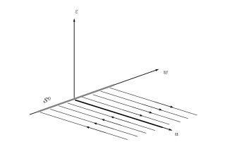
(a) Flow in $(u,w,\varepsilon)$-space; the thick gray line represents the critical manifold $\SS^{0}$.

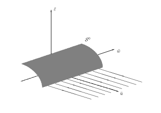
(b) Geometry in blown-up $(\bar{u},\bar{w},\bar{\varepsilon})$-space; $\SS^{0}$ is now represented by the cylinder corresponding to $\bar{u}^{2}+\bar{\varepsilon}^{2}=1$.

Figure 7: Flow of Equation 13 for $\varepsilon=0$ (a) before and (b) after the blow-up in Eq. 19.

The change of coordinates between charts $K_{1}$ and $K_{2}$, which we denote by $\kappa_{12}$, can be written as

(21) $$\kappa_{12}:\ (u_{2},w_{2},\xi_{2},r_{2})=\big{(}\varepsilon_{1}^{-1},w_{1},\xi_{1},r_{1}\varepsilon_{1}\big{)},$$

while its inverse $\kappa_{21}$ is given by

(22) $$\kappa_{21}:\ (r_{1},w_{1},\xi_{1},\varepsilon_{1})=\big{(}r_{2}u_{2},w_{2},\xi_{2},u_{2}^{-1}\big{)}.$$

To obtain the governing equations in $K_{1}$, we substitute the transformation from Eq. 20a into Equation 13; a straightforward calculation yields

(23a) $$r_{1}^{\prime} =r_{1}^{4}w_{1},$$

(23b) $$w_{1}^{\prime} =r_{1}^{3}\varepsilon_{1}(1-\varepsilon_{1}^{2}),$$

(23c) $$\xi_{1}^{\prime} =\delta r_{1}^{4},$$

(23d) $$\varepsilon_{1}^{\prime} =-r_{1}^{3}\varepsilon_{1}w_{1}.$$

Since $\varepsilon=r_{1}\varepsilon_{1}$, the singular limit of $\varepsilon=0$ corresponds to the restriction of the flow of Eq. 23 to one of the invariant planes $\{r_{1}=0\}$ or $\{\varepsilon_{1}=0\}$. In order to obtain a non-vanishing vector field for $r_{1}=0$, we desingularize Equation 23 by dividing out a factor of $r_{1}^{3}$ from the right-hand sides, which again represents a rescaling of the corresponding independent variable:

(24a) $$r_{1}^{\prime} =r_{1}w_{1},$$

(24b) $$w_{1}^{\prime} =\varepsilon_{1}(1-\varepsilon_{1}^{2}),$$

(24c) $$\xi_{1}^{\prime} =\delta r_{1},$$

(24d) $$\varepsilon_{1}^{\prime} =-\varepsilon_{1}w_{1}.$$

The governing equations in $K_{2}$ are obtained by substituting the transformation in Eq. 20b into Eq. 13, which gives

(25a) $$u_{2}^{\prime} =r_{2}^{3}u_{2}^{4}w_{2},$$

(25b) $$w_{2}^{\prime} =r_{2}^{3}(u_{2}^{2}-1),$$

(25c) $$\xi_{2}^{\prime} =\delta r_{2}^{4}u_{2}^{4}.$$

(25d) $$r_{2}^{\prime} =0.$$

Desingularizing as before, by dividing out a factor of $r_{2}^{3}$ from the right-hand sides in Eq. 25, we find

(26a) $$u_{2}^{\prime} =u_{2}^{4}w_{2},$$

(26b) $$w_{2}^{\prime} =u_{2}^{2}-1,$$

(26c) $$\xi_{2}^{\prime} =\delta r_{2}u_{2}^{4},$$

(26d) $$r_{2}^{\prime} =0.$$

Here, we remark that, by construction, the $(u_{2},w_{2})$-subsystem {Eq. 26a,Eq. 26b} corresponds to Equation 18.

Finally, we define various sections for the blown-up vector field, which will be used throughout the following analysis: in $K_{1}$, we will require the entry and exit sections

(27a) $$\Sigma_{1}^{\rm in} :=\big{\{}(\rho,w_{1},\xi_{1},\varepsilon_{1})\,\big{|}\,w_{1}\in[w_{-},w_{+}],\ \xi_{1}\in[\xi_{-},\xi_{+}],\text{ and }\varepsilon_{1}\in[0,\sigma]\big{\}}\quad\text{and}$$

(27b) $$\Sigma_{1}^{\rm out} :=\big{\{}(r_{1},w_{1},\xi_{1},\sigma)\,\big{|}\,r_{1}\in[0,\rho],\ w_{1}\in[w_{-},w_{+}],\text{ and }\xi_{1}\in[\xi_{-},\xi_{+}]\big{\}},$$

respectively, where $0<\rho<1$ and $0<\sigma<1$ are appropriately defined constants, while $w_{\mp}$ and $\xi_{\mp}$ are real constants, with $w_{-}<-\frac{2}{\sqrt{3}}$ and $w_{+}>\frac{2}{\sqrt{3}}$. Similarly, in chart $K_{2}$, we will employ the section

(28) $$\Sigma_{2}^{\rm in}:=\big{\{}(\sigma^{-1},w_{2},\xi_{2},r_{2})\,\big{|}\,w_{2}\in[w_{-},w_{+}],\ \xi_{2}\in[\xi_{-},\xi_{+}],\text{ and }r_{2}\in[0,\rho\sigma]\big{\}};$$

here, we note that $\Sigma_{2}^{\rm in}=\kappa_{21}\big{(}\Sigma_{1}^{\rm out}\big{)}$.

Equations 24 and 26 will allow us to construct solutions of {Eq. 13,Eq. 14}. Following the strategy outlined in Section 2, we will focus our attention on the $\xi$-interval $[-1,0]$ with boundary conditions $u(-1)=1$ and $w(0)=0$; in particular, and as indicated in Remark 3.1, the “outer” regime will be realized in terms of the flow between the sections $\Sigma_{1}^{\rm in}$ and $\Sigma_{1}^{\rm out}$ in chart $K_{1}$. Translating the resulting asymptotics into chart $K_{2}$ via the transformation in Equation 21, we will then construct solutions in the “inner” regime between the section $\Sigma_{2}^{\rm in}$ and the hyperplane corresponding to $\{w=0\}$.

Remark 3.2.

In the following, we will denote a given general variable $z$ in blown-up space with $\bar{z}$. In charts $K_{i}$, $i=1,2$ that variable will instead be labeled with the corresponding subscript, as $z_{i}$.

4 Analysis of Bifurcation Diagram – Proof of Theorem 1.2

In this section, we establish the bifurcation diagram in Fig. 3 for $\varepsilon$ positive and sufficiently small, proving Theorem 1.2. To that end, we investigate the existence and uniqueness of solutions to Equation 13, subject to the boundary conditions in Eq. 14.

All such solutions arise as perturbations of certain limiting solutions that are obtained in the limit of $\varepsilon=0$. We denote these limiting solutions as singular solutions, as is usual in geometric singular perturbation theory. The approach adopted thereby is the following: first, singular solutions are constructed by analyzing the dynamics in charts $K_{1}$ and $K_{2}$ separately in the limit as $\varepsilon\to 0$. Then, the persistence of singular solutions for non-zero $\varepsilon$ is shown via the shooting argument outlined in Section 2, which relies on the transversality of the geometric objects involved. That transversality translates into the existence of solutions to the boundary value problem {Eq. 13,Eq. 14} along the branches depicted in the bifurcation diagram in Fig. 3.

Definition 4.1.

We distinguish three types of singular solutions to the boundary value problem {Eq. 13,Eq. 14}; see Fig. 8:

Type I.

Solutions of type I satisfy $u=0$ for $x\in I$, where $I$ is an interval centered at $x=0$. Consequently, the slope of such solutions must initially satisfy $|w|>1$, in terms of the original $w$-variable. Type I-solutions, which will henceforth be illustrated in blue, occur in two subtypes: the ones corresponding to $\lambda=\mathcal{O}(\varepsilon)$ have constant finite slope $w$ outside of $I$, while the ones corresponding to $\lambda=\mathcal{O}(1)$ vanish on $I=(-1,1)$.

Type II.

Solutions of type II are those of slope $w\equiv\mp 1$, in terms of the original $w$-variable. These solutions exhibit “touchdown”, reaching $\{u=0\}$ at one point only, namely at $\xi=0$. Type II-solutions will be indicated in green in all subsequent figures.

Type III.

Solutions of type III never reach $\{u=0\}$; hence, no touchdown phenomena occur. These solutions correspond to solutions of the non-regularized model, with $\varepsilon=0$ in Equation 3 [24, 25].

Remark 4.2.

The usage of the plural in the definition of type II-solutions requires additional clarification. For Equation 7, there exists just one singular solution of type II for $\lambda=0$ with slope $w=\mp 1$; see the solution labeled $d$ in Figure Fig. 2. However, in our blow-up analysis, that singular solution corresponds to a one-parameter family of type II-solutions.

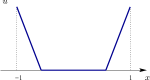
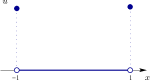
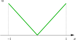
Figure 8: Singular solutions to Equation 13, as specified in Definition 4.1: (a) type I-solutions for $\lambda=\mathcal{O}(\varepsilon)$ (left panel) and $\lambda=\mathcal{O}(1)$ (right panel), (b) type II-solutions, and (c) type III-solutions.

For $\varepsilon>0$, we divide the bifurcation diagram in Fig. 3 into three overlapping regions, as shown in Fig. 9.

Remark 4.3.

Henceforth, we will refer to the norm $\|u\|_{2}^{2}$ in terms of the original variable $u$ in order to be able to compare our analysis with that in [20]; see Figs. 2 and 3.

Region $\mathcal{R}_{1}$ is defined as

(29) $$\mathcal{R}_{1}:=[0,1]\times\bigg{[}\frac{2}{3}+\nu_{1},2\bigg{]},\qquad\text{with }\nu_{1}>0;$$

that region covers the upper part of the bifurcation diagram, where we find the newly emergent branch of solutions for $\varepsilon>0$ in Eq. 3 by perturbing from singular solutions of type I. Region $\mathcal{R}_{2}$, which is defined as

(30) $$\mathcal{R}_{2}:=[0,\varepsilon\lambda_{2}]\times\bigg{[}\frac{2}{3}-\nu_{2},\frac{2}{3}+\nu_{2}\bigg{]},\qquad\text{with }\lambda_{2}>0\text{ and }\nu_{2}>0$$

for $\nu_{2}>\nu_{1}$ and $\lambda_{2}$ large, but fixed, represents a small neighborhood of the point $B$ that is depicted as a rectangle in Fig. 9. That region shrinks with decreasing $\varepsilon$, collapsing to the segment $\{0\}\times\big{[}\frac{2}{3}-\nu_{2},\frac{2}{3}+\nu_{2}\big{]}$ as $\varepsilon\to 0$. The branch of solutions contained in this “transition” region is constructed by perturbation from singular solutions of types I and II. Finally, region $\mathcal{R}_{3}$ is defined as

(31) $$\mathcal{R}_{3}:=[0,1]\times\bigg{[}0,\frac{2}{3}+\nu_{2}\bigg{]}\setminus[0,\varepsilon\lambda_{3}]\times\bigg{[}\frac{2}{3}-\nu_{3},\frac{2}{3}+\nu_{2}\bigg{]},\qquad\text{with }\lambda_{3}>0\text{ and }\nu_{3}>0,$$

where $\nu_{3}<\nu_{2}$ and $\lambda_{3}$ is again large, but fixed, with $\lambda_{3}<\lambda_{2}$. Region $\mathcal{R}_{3}$ covers the lower part of the bifurcation diagram in Fig. 3, and contains the branch of solutions which is obtained by perturbing from solutions of types II and III.

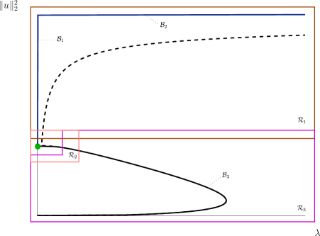
Figure 9: Covering of the bifurcation diagram for the boundary value problem {Eq. 13,Eq. 14} by three overlapping regions $\mathcal{R}_{1}$ (brown), $\mathcal{R}_{2}$ (pink), and $\mathcal{R}_{3}$ (magenta), for $\varepsilon$ positive and small. (For improved visibility, the regions have been extended slightly below $\|u\|_{2}^{2}=0$, above $\|u\|_{2}^{2}=2$, and to negative $\lambda$, respectively; also, we recall Remark 4.3 with regard to the interpretation of $\|u\|_{2}^{2}$ in this context.) The branches of solutions to the boundary value problem {Eq. 13,Eq. 14} for $\varepsilon=0.01$ (dotted curve) and $\varepsilon=0$ (solid curve) are also displayed. In $\mathcal{R}_{3}$, these branches overlap almost entirely. For $\varepsilon=0$, the blue branch reduces to the union of a vertical part $\mathcal{B}_{1}$, corresponding to $\lambda=\mathcal{O}(\varepsilon)$, and a horizontal part $\mathcal{B}_{2}$ which corresponds to $\lambda=\mathcal{O}(1)$. The green dot at $B$ represents the singular solution of type II for $\lambda=0$ that is labeled $d$ in Fig. 2. The black curve, corresponding to the branch of solutions to the non-regularized model, is labeled $\mathcal{B}_{3}$. In the limit as $\varepsilon\to 0$, $\mathcal{R}_{2}$ shrinks to a segment on the $\|u\|_{2}^{2}$-axis that contains the point $B$, cf. Eq. 30, while region $\mathcal{R}_{3}$ grows to a rectangle minus a smaller segment on the $\|u\|_{2}^{2}$-axis containing the point $B$; recall Eq. 31.

The true meaning of these regions becomes clearer when we consider a blow-up of the bifurcation diagram in parameter space, i.e., with respect to $\lambda$ and $\varepsilon$, as illustrated in Fig. 10. (That same point of view will also prove useful in parts of the following analysis.) We first embed the diagram, which depends on $(\lambda,\|u\|_{2}^{2})$, into $\mathbb{R}^{3}$ by including the third variable $\varepsilon$. Then, we blow up the line $\{(0,0)\}\times\mathbb{R}$ by introducing $\bar{r},\bar{\lambda}$, and $\bar{\varepsilon}$ such that

$$\lambda=\bar{r}\bar{\lambda}\qquad\text{and}\qquad\varepsilon=\bar{r}\bar{\varepsilon}$$

with $\bar{\lambda}^{2}+\bar{\varepsilon}^{2}=1$, i.e., for $(\bar{\lambda},\bar{\varepsilon})\in S^{1}$, and $\bar{r}\in[0,r_{0})$, where $r_{0}>0$. In the blown-up space $S^{1}\times\mathbb{R}^{2}$, the line $\{(0,0)\}\times\mathbb{R}$ is hence blown up to a cylinder $S^{1}\times\{0\}\times\mathbb{R}$.

After blow-up, the curve of singular solutions obtained for $\varepsilon=0$ consists of three portions which correspond to singular solutions of types I, II, and III, cf. Fig. 8, and which are shown in blue, green, and black, respectively. The black curve (type III) is located in $\bar{\varepsilon}=0$, while the green curve (type II) lies on the cylinder, i.e., in $\{\bar{r}=0\}$, with $\|u\|_{2}^{2}=\frac{2}{3}$ constant. Finally, the blue curve (type I) consists of a branch on the cylinder, corresponding to $\lambda=\mathcal{O}(\varepsilon)$, and of another branch in the plane $\{\bar{\varepsilon}=0\}$ that corresponds to $\lambda=\mathcal{O}(1)$. In the former case, type I-solutions resemble the one shown in the left panel of Fig. 8; in the second case, type I-solutions are as in the right panel of Fig. 8. These two branches correspond to $\mathcal{B}_{1}$ and $\mathcal{B}_{2}$, respectively, as defined in Fig. 9.

Loosely speaking, in blown-up space, a neighborhood of the green curve is hence covered by region $\mathcal{R}_{2}$ and part of $\mathcal{R}_{3}$. The blue curve is mostly covered by region $\mathcal{R}_{1}$, with a small portion close to $\delta=\frac{2}{\sqrt{3}}$ covered by $\mathcal{R}_{2}$. Finally, region $\mathcal{R}_{3}$ covers the remainder of the green curve close to $\delta=0$, and the black curve. The curve obtained for $0<\varepsilon\ll 1$, which is depicted in red in Fig. 10, lifts off from the singular curve corresponding to the limit of $\varepsilon=0$.

Remark 4.4.

When referring to regions $\mathcal{R}_{i}$, $i=1,2,3$, in blown-up space, we need to consider the preimages of $\mathcal{R}_{i}\times[0,\varepsilon_{0}]$ under the blow-up transformation defined above, strictly speaking. However, for the sake of simplicity, we will use the two notations interchangeably.

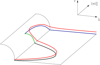
Figure 10: Bifurcation diagram for the boundary value problem {Eq. 13,Eq. 14} in blown-up parameter space. In the singular limit corresponding to $\varepsilon=0$, the diagram consists of the union of the blue, green, and black solid curves, which are covered by $\mathcal{R}_{1}$, $\mathcal{R}_{2}$, and $\mathcal{R}_{3}$, respectively. The portion of the blue curve which lies on the cylinder corresponds to the line $\mathcal{B}_{1}$, while the portion contained in the $\{\bar{\varepsilon}=0\}$-plane corresponds to $\mathcal{B}_{2}$. The red curve which lifts off from the {$\varepsilon=0$}-curve represents solutions to the boundary value problem {Eq. 13,Eq. 14} for $\varepsilon$ positive, but small.

As stated in Theorem 1.2, we consider $\lambda\in[0,\Lambda]$, where we take $\Lambda=1$ for the sake of simplicity. In region $\mathcal{R}_{3}$, away from the point $B$, the perturbation with $\varepsilon$ is regular. As will be shown below, singular solutions in regions $\mathcal{R}_{1}$ and $\mathcal{R}_{2}$ exist only for $\lambda\geq\frac{3}{4}\varepsilon$ or, equivalently, for $\delta\leq\frac{2}{\sqrt{3}}$; cf. Sections 4.1 and 4.2. Hence, in these regions, we need to take $\lambda\in\big{[}\frac{3}{4}\varepsilon,1\big{]}$, i.e.,

(32) $$\delta\in\bigg{[}\sqrt{\varepsilon},\frac{2}{\sqrt{3}}\bigg{]},$$

which corresponds to the region shaded in gray in Fig. 11.

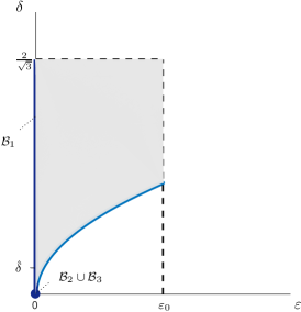
Figure 11: Region in $(\varepsilon,\delta)$-space, as considered in our analysis. The region, which is shaded in gray, is bounded from below by $\{\delta=\sqrt{\varepsilon}\}$ (light blue curve) and from above by $\{\delta=\frac{2}{\sqrt{3}}\}$ (dashed horizontal line); cf. Eq. 32. The dark blue segment of the $\delta$-axis corresponds to the union of the two portions of the blue curve shown in Figs. 9 and 10. The vertical line corresponds to the line $\mathcal{B}_{1}$, which is divided into two segments at some $\hat{\delta}>0$ small, while the dot corresponds to the curve $\mathcal{B}_{2}\cup\mathcal{B}_{3}$.

As evidenced in Fig. 11, $\delta=0$ occurs only when $\varepsilon=0$, which is the point represented by the blue dot therein. The corresponding, highly degenerate limit gives a singular orbit of type I with very singular structure, as shown in the right panel in Fig. 8. Hence, the whole line $\mathcal{B}_{2}$ in the bifurcation diagram for $\varepsilon=0$ shown in Fig. 9 corresponds to that one singular solution.

4.1 Region $\mathcal{R}_{1}$

Region $\mathcal{R}_{1}$ in the bifurcation diagram in Fig. 9 corresponds to solutions that reduce to those of type I in the singular limit; cf. Definition 4.1. For $\varepsilon$ positive and sufficiently small, solutions on that branch come very close to $\{u=\varepsilon\}$; moreover, the length of the interval $I$ where $u\approx\varepsilon$ grows with $\lambda$. In the singular limit of $\varepsilon=0$, the slope of the respective solutions is moderate for $\lambda=\mathcal{O}(\varepsilon)$, corresponding to $0<\delta<\frac{2}{\sqrt{3}}$, while it tends to infinity for $\lambda=\mathcal{O}(1)$ – i.e., as $\delta\to 0$ – along the two segments where $u$ changes from $u=0$ to $u=1$. These observations are confirmed by the rescaling of $w$ in Eq. 11: for $\lambda=\mathcal{O}(\varepsilon)$, that rescaling translates into $w=\mathcal{O}(1)$, while it gives $w\to\infty$ for $\lambda=\mathcal{O}(1)$; cf. Fig. 8. Interestingly, the proof of our main result in this section, which is stated below, is very similar for these two $\lambda$-regimes:

Proposition 4.5.

Given $\delta_{1}$ fixed, with $0<\delta_{1}<\frac{2}{\sqrt{3}}$ and $\delta_{1}\approx\frac{2}{\sqrt{3}}$, there exists $\varepsilon_{0}>0$ sufficiently small such that in region $\mathcal{R}_{1}$, the boundary value problem {Eq. 13,Eq. 14} has a unique branch of solutions for $\varepsilon\in(0,\varepsilon_{0})$ and $\lambda\in\big{[}\frac{\varepsilon}{\delta_{1}^{2}},1\big{]}$. As $\varepsilon\to 0$, these solutions limit on a singular solution $\Gamma$ of type I.

Remark 4.6.

The singular solution $\Gamma$ depends on $\lambda$ or, equivalently, on $\delta$. Interpreted in terms of $\delta$, the range for which singular solutions exist corresponds to $\delta\in\big{[}\sqrt{\varepsilon},\delta_{1}\big{]}$; recall Eq. 12.

To prove Proposition 4.5, we construct solutions corresponding to the branch that is contained in region $\mathcal{R}_{1}$ for fixed $\lambda$ in the regime considered here. For $\delta$ fixed, a unique singular orbit $\Gamma$ is determined in blown-up phase space by investigating the dynamics of the boundary value problem {Eq. 13,Eq. 14} separately in charts $K_{1}$ and $K_{2}$, and by then combining the results obtained in these charts. Finally, the singular orbit $\Gamma$, which is essentially determined by the dynamics in chart $K_{2}$, is shown to persist for $\varepsilon$ positive and sufficiently small.

4.1.1 Dynamics in chart $K_{2}$

The flow of Equation 13 from the section $\Sigma_{2}^{\rm in}$ back to itself, whereby the sign of $w$ changes from negative to positive, is naturally described in chart $K_{2}$; cf. Fig. 12.

Recalling that $r_{2}=\varepsilon$, we observe that Equation 26 constitutes a fast-slow system in the standard form of geometric singular perturbation theory [7, 10, 15], with $(u_{2},w_{2})$ the fast variables and $\xi_{2}$ the slow variable. The fast system is given by Eq. 26, whence the corresponding slow system is obtained by a rescaling of the independent variable with $r_{2}$:

(33a) $$r_{2}\dot{u}_{2} =u_{2}^{4}w_{2},$$

(33b) $$r_{2}\dot{w}_{2} =u_{2}^{2}-1,$$

(33c) $$\dot{\xi}_{2} =\delta u_{2}^{4},$$

(33d) $$\dot{r}_{2} =0.$$

The associated layer and reduced problems, which are obtained by setting $r_{2}=0$ in Eq. 26 and Eq. 33, respectively, read

(34a) $$u_{2}^{\prime} =u_{2}^{4}w_{2},$$

(34b) $$w_{2}^{\prime} =u_{2}^{2}-1,$$

(34c) $$\xi_{2}^{\prime} =0,$$

(34d) $$r_{2}^{\prime} =0$$

and

(35a) $$0 =u_{2}^{4}w_{2},$$

(35b) $$0 =u_{2}^{2}-1,$$

(35c) $$\dot{\xi}_{2} =\delta u_{2}^{4},$$

(35d) $$\dot{r}_{2} =0,$$

respectively. (We note that the $(u_{2},w_{2})$-subsystem {Eq. 34a,Eq. 34b} is precisely equal to Equation 18.) The critical manifold for Equation 35 is given by the line

(36) $$\SS_{2}^{0}:=\big{\{}(1,0,\xi_{2},0)\,\big{|}\,\xi_{2}\in[\xi_{-},\xi_{+}]\big{\}},$$

where the constants $\xi_{\mp}$ are defined as before.

Remark 4.7.

While steady states are also found for $u_{2}=-1$ in Eq. 26, these states are irrelevant, since $u_{2}$ and $r_{2}$ are both non-negative and since $\{u_{2}=0\}$ is an invariant hyperplane for Eq. 26 which the flow cannot cross.

Linearization of Eq. 34 about the critical manifold $\SS_{2}^{0}$ shows that any point $Q_{2}=(1,0,\xi_{2},0)\in\SS_{2}^{0}$ is a saddle, with Jacobian

$$\Bigg{[}\begin{array}[]{cc}4u_{2}^{3}w_{2}&u_{2}^{4}\\ 2u_{2}&0\end{array}\Bigg{]}\Bigg{|}_{(u_{2},w_{2})=(1,0)}=\Bigg{[}\begin{array}[]{cc}0&1\\ 2&0\end{array}\Bigg{]}$$

and eigenvalues $\pm\sqrt{2}$. Hence, the manifold $\SS_{2}^{0}$ is normally hyperbolic. The reduced flow thereon is described by $\dot{\xi}_{2}=\delta$, which corresponds to a constant drift in the positive $u_{2}$-direction with speed $\delta$.

To describe the integrable layer flow away from $\SS_{2}^{0}$, we introduce $u_{2}$ as the independent variable, dividing Eq. 34b formally by Eq. 34a:

$$\frac{{\rm d}w_{2}}{{\rm d}u_{2}}=\frac{u_{2}^{2}-1}{u_{2}^{4}w_{2}(u_{2})}.$$

Solving the above equation with $w_{2}(1)=0$, we find

(37) $$w_{2}^{\mp}(u_{2})=\mp\sqrt{\frac{4}{3}-\frac{2}{u_{2}}+\frac{2}{3u_{2}^{3}}}.$$

In particular, it follows from Eq. 37 that, for any fixed choice of $\xi_{2}$, the stable and unstable manifolds of $Q_{2}$ can be written as graphs over $u_{2}$:

(38a) $$\mathcal{W}_{2}^{\rm s}(Q_{2}) =\big{\{}(u_{2},w_{2}^{-}(u_{2}),\xi_{2},0)\,\big{|}\,u_{2}\in[1,\infty)\big{\}},$$

(38b) $$\mathcal{W}_{2}^{\rm u}(Q_{2}) =\big{\{}(u_{2},w_{2}^{+}(u_{2}),\xi_{2},0)\,\big{|}\,u_{2}\in[1,\infty)\big{\}}.$$

We have the following result.

Lemma 4.8.

Let $r_{2}\in(0,r_{0})$, with $r_{0}$ positive and sufficiently small. Then, the following statements hold for Equation 33:

1. The normally hyperbolic critical manifold $\SS_{2}^{0}$ perturbs to a slow manifold

   $$\SS_{2}^{r_{2}}=\big{\{}(1,0,\xi_{2},r_{2})\,\big{|}\,\xi_{2}\in[\xi_{-},\xi_{+}]\big{\}},$$

   where $\xi_{\mp}$ are appropriately chosen constants. In particular, we emphasize that $(u_{2},w_{2})=(1,0)\in\SS_{2}^{r_{2}}$.

2. The corresponding stable and unstable foliations $\mathcal{F}_{2}^{\rm s}(\SS_{2}^{r_{2}})$ and $\mathcal{F}_{2}^{\rm u}(\SS_{2}^{r_{2}})$ are identical to $\mathcal{F}_{2}^{\rm s}(\SS_{2}^{0})$ and $\mathcal{F}_{2}^{\rm u}(\SS_{2}^{0})$, except for their constant $r_{2}$-component. For $r_{2}\in[0,r_{0})$ fixed, these foliations may be written as

   (39a) $$\mathcal{F}_{2}^{\rm s}(\SS_{2}^{r_{2}}) =\big{\{}(u_{2},w_{2}^{-}(u_{2}),\xi_{2},r_{2})\,\big{|}\,u_{2}\in[1,\infty),\ \xi_{2}\in[\xi_{-},\xi_{+}]\big{\}}\quad\text{and}$$

   (39b) $$\mathcal{F}_{2}^{\rm u}(\SS_{2}^{r_{2}}) =\big{\{}(u_{2},w_{2}^{+}(u_{2}),\xi_{2},r_{2})\,\big{|}\,u_{2}\in[1,\infty),\ \xi_{2}\in[\xi_{-},\xi_{+}]\big{\}}.$$

Proof 4.9.

Both statements follow immediately from standard geometric singular perturbation theory [7], in combination with the preceding analysis; in particular, the fact that the plane $\{(u_{2},w_{2})=(1,0)\}$ is invariant for Equation 26 irrespective of the choice of $r_{2}$ implies that the restrictions of $\SS_{2}^{r_{2}}$ and $\SS_{2}^{0}$ to $(u_{2},w_{2},\xi_{2})$-space do not depend on $r_{2}$.

Remark 4.10.

The fast-slow structure of Equation 26 is very simple, since the $(u_{2},w_{2})$-subsystem {Eq. 26a,Eq. 26b} decouples from Equation 26c. Even for $\varepsilon>0$, the fast dynamics is determined by that integrable planar system, and organized by the saddle point at $(1,0)$ and the stable and unstable manifolds thereof. The slow flow on the slow manifold $\SS_{2}^{r_{2}}$ is just the drift given by $\dot{\xi}=\delta$.

In the limit as $u_{2}\to\infty$, $w_{2}^{\mp}(u_{2})$ converges to $w_{2}^{\mp}(\infty)=\mp\frac{2}{\sqrt{3}}$; recall Eq. 37. Transforming the stable manifold $\mathcal{W}_{2}^{\rm s}(Q_{2})$ and the unstable manifold $\mathcal{W}_{2}^{\rm u}(Q_{2})$ to chart $K_{1}$, via the coordinate change $\kappa_{21}$ defined in Eq. 22, we see that these manifolds limit on the points $\big{(}0,\mp\frac{2}{\sqrt{3}},\xi_{1},0\big{)}$, respectively, for $\xi_{1}$ fixed; see Fig. 12.

4.1.2 Dynamics in chart $K_{1}$

The portions of the singular orbit $\Gamma$ corresponding to the flow between two sets of boundary conditions that are located at $\xi=\mp 1$ and the section $\Sigma_{1}^{\rm out}$ are studied in chart $K_{1}$. A simple calculation reveals that Equation 24 admits a line of steady states at

(40) $$\SS_{1}^{0}:=\big{\{}(0,0,\xi_{1},1)\,\big{|}\,\xi_{1}\in[\xi_{-},\xi_{+}]\big{\}},$$

as well as the plane of steady states

(41) $$\pi_{1}:=\big{\{}(0,w_{1},\xi_{1},0)\,\big{|}\,w_{1}\in[w_{-},w_{+}]\text{ and }\xi_{1}\in[\xi_{-},\xi_{+}]\big{\}};$$

here, $w_{\mp}$ and $\xi_{\mp}$ are defined as in Eq. 27. (Another set of equilibria, with $\varepsilon_{1}=-1$, is irrelevant to us due to our assumption that $r_{1}$ and $\varepsilon_{1}$ are both non-negative.) The line $\SS_{1}^{0}$ corresponds to the saddle equilibrium at $(\hat{u},w)=(1,0)$ of Equation 18, and coincides with the critical manifold $\SS_{2}^{0}$ introduced in chart $K_{2}$; cf. Equation 36.

In chart $K_{1}$, the singular limit of $\varepsilon=0$ corresponds to either $r_{1}=0$ or $\varepsilon_{1}=0$ in Equation 24, which yields the following two limiting systems in the corresponding invariant hyperplanes:

(42a) $$r_{1}^{\prime} =0,$$

(42b) $$w_{1}^{\prime} =\varepsilon_{1}(1-\varepsilon_{1}^{2}),$$

(42c) $$\xi_{1}^{\prime} =0,$$

(42d) $$\varepsilon_{1}^{\prime} =-\varepsilon_{1}w_{1}$$

and

(43a) $$r_{1}^{\prime} =r_{1}w_{1},$$

(43b) $$w_{1}^{\prime} =0,$$

(43c) $$\xi_{1}^{\prime} =\delta r_{1},$$

(43d) $$\varepsilon_{1}^{\prime} =0,$$

respectively. Equation 42 is equivalent to Equation 34 in chart $K_{2}$ under the coordinate change $\kappa_{21}$ defined in Eq. 22; these equations describe the portion of the singular orbit $\Gamma$ in chart $K_{1}$ that is located between $\Sigma_{1}^{\rm out}$ and the hyperplane $\{\varepsilon_{1}=0\}$. Equation 43, on the other hand, determines the portion of the singular orbit which connects the hyperplane $\{r_{1}=0\}$ with the boundary conditions imposed at $r_{1}=1$. Hence, we first focus our attention on that limiting system.

The value of $w_{1}$ in Equation 43 is constant: $w_{1}\equiv w_{0}$, for some constant $w_{0}$. Since $w_{0}$ must match the $w_{2}$-value obtained in the limit $u_{2}\to\infty$ in Eq. 37 in chart $K_{2}$, see Fig. 12, $w_{1}\equiv\mp\frac{2}{\sqrt{3}}$ must hold in the hyperplane $\{\varepsilon_{1}=0\}$. The corresponding orbits of Eq. 43 are then easily found by dividing Eq. 43c formally by Eq. 43a: $\frac{{\rm d}\xi_{1}}{{\rm d}r_{1}}=\frac{\delta}{w_{0}}$. For any initial condition $\xi_{1}(1)=\xi_{0}$, the solution to that equation reads

(44) $$\xi_{1}(r_{1})=\frac{\delta}{w_{0}}(r_{1}-1)+\xi_{0}.$$

The boundary conditions in Eq. 14 imply $\xi_{0}=\mp 1$; hence, and since $w_{0}=\mp\frac{2}{\sqrt{3}}$, we obtain

(45) $$\xi_{1}^{\mp}(r_{1})=\mp\frac{\sqrt{3}}{2}\delta(r_{1}-1)\mp 1.$$

Any orbit of Eq. 43 can then be written as

(46) $$\bigg{\{}\bigg{(}r_{1},\mp\frac{2}{\sqrt{3}},\xi_{1}^{\mp}(r_{1}),0\bigg{)}\,\bigg{|}\,r_{1}\in[0,1]\bigg{\}}.$$

Orbits of the integrable Equation 42 can be found by introducing $\varepsilon_{1}$ as the independent variable: dividing Eq. 42b formally by Eq. 42d, we obtain $\frac{{\rm d}w_{1}}{{\rm d}\varepsilon_{1}}=-\frac{1-\varepsilon_{1}^{2}}{w_{1}(\varepsilon_{1})}$, which can be solved explicitly with $w_{1}(0)=\mp\frac{2}{\sqrt{3}}$ to yield

(47) $$w_{1}^{\mp}(\varepsilon_{1})=\mp\sqrt{\frac{4}{3}-2\varepsilon_{1}+\frac{2}{3}\varepsilon_{1}^{3}},$$

where the sign in Eq. 47 equals that of the initial $w_{1}$-value. (We remark that Eq. 47 corresponds to Equation 37, after transformation to $K_{1}$-coordinates.) The corresponding values of $\xi_{1}$ are constant, and must equal the respective values of $\xi_{1}^{\mp}(r_{1})$ in Eq. 45 at $r_{1}=0$, i.e.,

(48) $$\xi_{1}^{\mp}(0)=\pm\frac{\sqrt{3}}{2}\delta\mp 1.$$

Remark 4.11.

For $\delta=\frac{2}{\sqrt{3}}$, it follows that $\xi_{1}^{\mp}(0)=0$, i.e., we obtain a singular orbit of type II; see Figs. 8 and 15. Hence, we must assume $\delta<\frac{2}{\sqrt{3}}$ in the statement of Proposition 4.5.

Any orbit of Eq. 42 can thus be represented as

(49) $$\big{\{}(0,w_{1}^{\mp}(\varepsilon_{1}),\xi_{1}^{\mp}(0),\varepsilon_{1})\,\big{|}\,\varepsilon_{1}\in[0,\sigma]\big{\}},$$

where $\sigma$ is as in the definition of the section $\Sigma_{1}^{\rm out}$; recall Eq. 27.

Concatenation of the two orbit segments defined in Equations 46 and 49 with the respective signs will yield the singular orbits $\Gamma_{1}^{-}$ and $\Gamma_{1}^{+}$, which are located between the sections $\mathcal{V}_{1_{0}}^{-}$ and $\Sigma_{1}^{\rm out}$ and $\Sigma_{1}^{\rm out}$ and $\mathcal{V}_{1_{0}}^{+}$, respectively. Here,

(50) $$\mathcal{V}_{1_{0}}^{\mp}:=\big{\{}(1,w,\mp 1,0)\,\big{|}\,w\in I^{\mp}\big{\}},$$

with $I^{\mp}$ being appropriately defined neighborhoods of the points $w_{0}^{-}=-\frac{2}{\sqrt{3}}$ and $w_{0}^{+}=\frac{2}{\sqrt{3}}$, respectively; see Fig. 12.

4.1.3 Singular orbit $\Gamma$

A singular orbit $\Gamma$ for Equation 13 can now be constructed on the basis of the dynamics in charts $K_{1}$ and $K_{2}$, by taking into account the corresponding boundary conditions in Equation 14.

After transformation to $K_{1}$, the manifolds $\mathcal{W}_{2}^{\rm s}(Q_{2})$ and $\mathcal{W}_{2}^{\rm u}(Q_{2})$ meet the portions of the orbits $\Gamma_{1}^{-}$ and $\Gamma_{1}^{+}$, respectively, as given by Eq. 49, in the points

(51) $$P_{1}^{\mp}=\bigg{(}0,\mp\frac{2}{\sqrt{3}},\pm\frac{\sqrt{3}}{2}\delta\mp 1,0\bigg{)}.$$

These points are contained in the two lines

(52a) $$\ell_{1}^{-} =\big{\{}(0,-\tfrac{2}{\sqrt{3}},\xi_{1},0)\,\big{|}\,\xi_{1}\in[\xi_{-},\xi_{+}]\big{\}}\quad\text{and}$$

(52b) $$\ell_{1}^{+} =\big{\{}(0,\tfrac{2}{\sqrt{3}},\xi_{1},0)\,\big{|}\,\xi_{1}\in[\xi_{-},\xi_{+}]\big{\}},$$

respectively, in the hyperplane $\{\varepsilon_{1}=0\}$, which are both located in the plane of steady states $\pi_{1}$; cf. Eq. 41. The portions of the singular orbit $\Gamma$ that lie in chart $K_{1}$ can hence finally be written as

(53a) $$\begin{split}\Gamma_{1}^{-}&=\big{\{}(r_{1},-\tfrac{2}{\sqrt{3}},-\tfrac{\sqrt{3}}{2}\delta(r_{1}-1)-1,0)\,\big{|}\,r_{1}\in(0,1]\big{\}}\cup P_{1}^{-}\\ &\cup\big{\{}(0,-\sqrt{\tfrac{4}{3}-2\varepsilon_{1}+\tfrac{2}{3}\varepsilon_{1}^{3}},\tfrac{\sqrt{3}}{2}\delta-1,\varepsilon_{1})\,\big{|}\,\varepsilon_{1}\in(0,\sigma]\big{\}}\quad\text{and}\end{split}$$

(53b) $$\begin{split}\Gamma_{1}^{+}&=\big{\{}(r_{1},\tfrac{2}{\sqrt{3}},\tfrac{\sqrt{3}}{2}\delta(r_{1}-1)+1,0)\,\big{|}\,r_{1}\in(0,1]\big{\}}\cup P_{1}^{+}\\ &\cup\big{\{}(0,\sqrt{\tfrac{4}{3}-2\varepsilon_{1}+\tfrac{2}{3}\varepsilon_{1}^{3}},-\tfrac{\sqrt{3}}{2}\delta+1,\varepsilon_{1})\,\big{|}\,\varepsilon_{1}\in(0,\sigma]\big{\}}.\end{split}$$

It remains to identify the portion of $\Gamma$ that is located in chart $K_{2}$; we denote the corresponding singular orbit by $\Gamma_{2}$. We note that, for $r_{2}=0$, Equation 34 implies $\xi_{2}\equiv{\rm constant}$ on $\Gamma_{2}$. Given the definition of $\Gamma_{1}^{\mp}$ and the fact that $\xi_{2}=\xi_{1}$, we define the points

(54) $$Q_{2}^{\mp}=\bigg{(}1,0,\pm\frac{\sqrt{3}}{2}\delta\mp 1,0\bigg{)}\in\SS_{2}^{0};$$

therefore, we may write

(55) $$\Gamma_{2}=\mathcal{W}_{2}^{\rm s}(Q_{2}^{-})\cup Q_{2}^{-}\cup\big{\{}(1,0,\xi_{2},0)\,\big{|}\,\xi_{2}\in(\tfrac{\sqrt{3}}{2}\delta-1,-\tfrac{\sqrt{3}}{2}\delta+1)\big{\}}\cup Q_{2}^{+}\cup\mathcal{W}_{2}^{\rm u}(Q_{2}^{+}),$$

recall Equation 38, where $u_{2}$ now varies in the range $[1,\sigma^{-1}]$. The orbit $\Gamma_{2}$ is hence defined as the union of three segments, with the first being the stable manifold of $Q_{2}^{-}$, the second corresponding to the slow drift in $\xi_{2}$ from $Q_{2}^{-}$ to $Q_{2}^{+}$, as shown in the inset of Fig. 12, and the third being the unstable manifold of $Q_{2}^{+}$.

The sought-after singular orbit $\Gamma$, which represents the singular solution to the boundary value problem {Eq. 13,Eq. 14}, can then be written as the union of $\Gamma_{1}^{-}$, $\Gamma_{2}$, and $\Gamma_{1}^{+}$ in blown-up space:

$$\Gamma:=\Gamma_{1}^{-}\cup\Gamma_{2}\cup\Gamma_{1}^{+}.$$

A visualization of the orbit $\Gamma$ is given in Fig. 12.

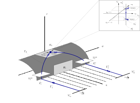
Figure 12: Geometry of the singular orbit $\Gamma=\Gamma_{1}^{-}\cup\Gamma_{2}\cup\Gamma_{1}^{+}$ for Equation 13 in blown-up space. The orbit $\Gamma$ is shown in blue, corresponding to a singular solution of type I. The inset resolves in detail the fast-slow structure in $(u_{2},w_{2},\xi_{2})$-space in chart $K_{2}$; in particular, the critical manifold $\SS_{2}^{0}$ and the resulting singular connection between $Q_{2}^{-}$ and $Q_{2}^{+}$ is shown.

4.1.4 Persistence of $\Gamma$ – Proof of Proposition 4.5

The proof of Proposition 4.5 is based on the shooting argument outlined in Section 2, which is implemented by approximating the dynamics of Equation 13 for $\varepsilon$ small in the two coordinate charts $K_{1}$ and $K_{2}$. We begin by defining the two manifolds

(56) $$\mathcal{V}_{1_{\varepsilon}}^{\mp}:=\big{\{}(1,w,\mp 1,\varepsilon)\,\big{|}\,w\in I^{\mp}\big{\}}\qquad\text{for }\varepsilon\in[0,\varepsilon_{0}),$$

which represent the boundary conditions in Eq. 14 in chart $K_{1}$, with $r_{1}=1$ for $\xi_{1}=\mp 1$; hence, it also follows that $\varepsilon_{1}=\frac{\varepsilon}{r_{1}}=\varepsilon$ there. (We note that, for $\varepsilon=0$, the manifolds $\mathcal{V}_{1_{\varepsilon}}^{\mp}$ in Eq. 56 reduce to $\mathcal{V}_{1_{0}}^{\mp}$, respectively, as defined in Eq. 50.) The intervals $I^{-}$ and $I^{+}$ are defined as neighborhoods of the points $w_{0}^{-}=-\frac{2}{\sqrt{3}}$ and $w_{0}^{+}=\frac{2}{\sqrt{3}}$, respectively, as before.

We note that the manifolds $\mathcal{V}_{1_{\varepsilon}}^{\mp}$ are mapped onto each other by the transformation $(r_{1},w_{1},\xi_{1},\varepsilon_{1})\mapsto(r_{1},-w_{1},-\xi_{1},\varepsilon_{1})$, in accordance with the symmetry properties of the boundary value problem {Eq. 13,Eq. 14}, as discussed in Section 1. It is hence sufficient to consider the transition from $\mathcal{V}_{1_{\varepsilon}}^{-}$ to $\Sigma_{1}^{\rm out}$ under the flow of Eq. 24, as its counterpart, the transition between $\Sigma_{1}^{\rm out}$ and $\mathcal{V}_{1_{\varepsilon}}^{+}$, can be obtained in a symmetric fashion.

We now introduce $\varepsilon_{1}$ as the independent variable in Equation 24, whence

(57a) $$\frac{{\rm d}r_{1}}{{\rm d}\varepsilon_{1}} =-\frac{r_{1}}{\varepsilon_{1}},$$

(57b) $$\frac{{\rm d}w_{1}}{{\rm d}\varepsilon_{1}} =-\frac{1-\varepsilon_{1}^{2}}{w_{1}(\varepsilon_{1})},$$

(57c) $$\frac{{\rm d}\xi_{1}}{{\rm d}\varepsilon_{1}} =-\delta\frac{r_{1}(\varepsilon_{1})}{\varepsilon_{1}w_{1}(\varepsilon_{1})}.$$

Here, we remark that $w_{1}(\varepsilon_{1})$ remains non-zero for $\varepsilon$ sufficiently small, as we know that $w_{1}=\mp\frac{2}{\sqrt{3}}+\mathcal{O}(\varepsilon_{1})\neq 0$ in the singular limit, i.e., for $\varepsilon=0$. Solving Equations 57a and 57b, with initial condition $(1,w,-1,\varepsilon)\in\mathcal{V}_{1_{\varepsilon}}^{-}$, we find

(58) $$r_{1}(\varepsilon_{1})=\frac{\varepsilon}{\varepsilon_{1}}\quad\text{and}\quad w_{1}^{-}(\varepsilon_{1})=-\sqrt{w^{2}+2(\varepsilon-\varepsilon_{1})-\frac{2}{3}(\varepsilon^{3}-\varepsilon_{1}^{3})}.$$

Substituting the expressions in Eq. 58 into Eq. 57c and expanding the result for $\varepsilon_{1}$ small, we obtain

$$\frac{{\rm d}\xi_{1}}{{\rm d}\varepsilon_{1}} =\delta\frac{\varepsilon}{\varepsilon_{1}^{2}}\frac{1}{\sqrt{w^{2}+2(\varepsilon-\varepsilon_{1})-\frac{2}{3}(\varepsilon^{3}-\varepsilon_{1}^{3})}}$$

$$=\delta\frac{\varepsilon}{\varepsilon_{1}}\frac{1}{\sqrt{w^{2}+2\varepsilon-\frac{2}{3}\varepsilon^{3}}}\bigg{[}\frac{1}{\varepsilon_{1}}+\frac{1}{w^{2}+2\varepsilon-\frac{2}{3}\varepsilon^{3}}\bigg{]}+\mathcal{O}(1),$$

which can be solved to the order considered here and evaluated in $\Sigma_{1}^{\rm out}$ – i.e., for $\varepsilon_{1}=\sigma$ – to yield

(59) $$\xi_{1}^{{\rm out}-}=-1-\frac{\delta}{w}+\frac{\delta}{w^{3}}\varepsilon\ln\varepsilon+\mathcal{O}(\varepsilon).$$

Similarly, evaluating Eq. 58 in $\Sigma_{1}^{\rm out}$, we find

$$\big{(}r_{1}^{{\rm out}-},w_{1}^{{\rm out}-},\xi_{1}^{{\rm out}-},\varepsilon_{1}^{{\rm out}-}\big{)}\\ =\bigg{(}\frac{\varepsilon}{\sigma},-\sqrt{w^{2}+2(\varepsilon-\sigma)-\frac{2}{3}(\varepsilon^{3}-\sigma^{3})},-1-\frac{\delta}{w}+\mathcal{O}(\varepsilon\ln\varepsilon),\sigma\bigg{)},$$

which defines a curve $(w_{1}^{{\rm out}-},\xi_{1}^{{\rm out}-})(w)$ that is parametrized by the initial $w_{1}$-value $w$ in $\mathcal{V}_{1_{\varepsilon}}^{-}$. That curve, which we denote by $\mathcal{V}_{1_{\varepsilon}}^{{\rm out}-}$, is located in a two-dimensional subset of $\Sigma_{1}^{\rm out}$ and, specifically, in the $(w_{1},\xi_{1})$-plane, with $(r_{1},\varepsilon_{1})$ fixed:

(60) $$\mathcal{V}_{1_{\varepsilon}}^{{\rm out}-}:=\bigg{\{}\bigg{(}-\sqrt{w^{2}+2(\varepsilon-\sigma)-\frac{2}{3}(\varepsilon^{3}-\sigma^{3})},-1-\frac{\delta}{w}+\mathcal{O}(\varepsilon\ln\varepsilon)\bigg{)}\,\bigg{|}\,w\in I^{-}\bigg{\}}.$$

It remains to study the stable foliation $\mathcal{F}_{2}^{\rm s}(\SS_{2}^{r_{2}})$ in coordinate chart $K_{2}$, and to show that the intersection thereof with $\mathcal{V}_{1_{\varepsilon}}^{{\rm out}-}$ is transverse for $\varepsilon$ sufficiently small. To that end, we recall the definition of $\mathcal{F}_{2}^{\rm s}(\SS_{2}^{r_{2}})$ in Eq. 39a, which we restrict to the section $\Sigma_{2}^{\rm in}=\kappa_{12}(\Sigma_{1}^{\rm out})$: taking $r_{2}(=\varepsilon)$ fixed, as before, and evaluating $\mathcal{F}_{2}^{\rm s}(\SS_{2}^{r_{2}})$ at $u_{2}=\sigma^{-1}$ defines a curve $\mathcal{F}_{2}^{{\rm in}-}$ in $\Sigma_{2}^{\rm in}$ which is parametrized by $\xi_{2}\in[\xi_{-},\xi_{+}]$ via

$$(u_{2}^{\rm in},w_{2}^{\rm in},\xi_{2}^{\rm in},r_{2}^{\rm in})=\Big{(}\sigma^{-1},-\sqrt{\tfrac{4}{3}-2\sigma+\tfrac{2}{3}\sigma^{3}},\xi_{2},r_{2}\Big{)},$$

for any $r_{2}\in[0,\rho\sigma]$; cf. Eq. 28. Transforming $\mathcal{F}_{2}^{{\rm in}-}$ to chart $K_{1}$, we obtain the corresponding curve $\mathcal{F}_{1}^{{\rm in}-}$:

(61) $$\mathcal{F}_{1}^{{\rm in}-}:=(w_{1}^{\rm out},\xi_{1}^{\rm out})=\bigg{\{}\bigg{(}-\sqrt{\frac{4}{3}-2\sigma+\frac{2}{3}\sigma^{3}},\xi_{1}\bigg{)}\,\bigg{|}\,\xi_{1}\in[\xi_{-},\xi_{+}]\bigg{\}}.$$

Comparing Equations 60 and 61 and expanding

$$-\sqrt{w^{2}+2(\varepsilon-\sigma)-\tfrac{2}{3}(\varepsilon^{3}-\sigma^{3})}=w+\frac{\varepsilon-\sigma}{w}+\mathcal{O}[(\varepsilon-\sigma)^{2}]$$

and

$$-\sqrt{\tfrac{4}{3}-2\sigma+\tfrac{2}{3}\sigma^{3}}=-\frac{2}{\sqrt{3}}+\frac{\sqrt{3}}{2}\sigma+\mathcal{O}(\sigma^{2}),$$

we conclude that $\mathcal{V}_{1_{\varepsilon}}^{{\rm out}-}$ and $\mathcal{F}_{1}^{{\rm in}-}$ intersect in some point

$$P_{1}^{{\rm out}-}=\bigg{(}-\frac{2}{\sqrt{3}}+\mathcal{O}(\varepsilon),-1-\frac{\delta}{w}+\mathcal{O}(\varepsilon\ln\varepsilon)\bigg{)}.$$

As the corresponding tangent vectors in the $(w_{1},\xi_{1})$-plane are given by $(1,\frac{\delta}{w^{2}})$ and $(0,1)$ to leading order, that intersection is transverse for any $\varepsilon$ small. More precisely, transversality between $\mathcal{V}_{1_{\varepsilon}}^{{\rm out}-}$ and $\mathcal{F}_{1}^{{\rm in}-}$ occurs already for $\varepsilon=0$, i.e., in $\{r_{1}=0\}$, which is sufficient for the Exchange Lemma to apply in chart $K_{2}$; cf. Fig. 13. As these two curves perturb smoothly, the transversality of their intersection persists for $\varepsilon\neq 0$, as well.

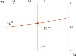
Figure 13: Transverse intersection of the sets $\mathcal{V}_{1_{0}}^{{\rm out}-}$ and $\mathcal{F}_{1}^{{\rm in}-}$ in $(w_{1},\xi_{1})$-space.

Next, and as stated above, the symmetry of Equation 24 implies the existence of a point $P_{1}^{{\rm out}+}=\big{(}\frac{2}{\sqrt{3}}+\mathcal{O}(\varepsilon),1-\frac{\delta}{w}+\mathcal{O}(\varepsilon\ln\varepsilon)\big{)}$ in $\Sigma_{1}^{\rm out}$ in which the curves

$$\mathcal{V}_{1_{\varepsilon}}^{{\rm out}+}=\bigg{\{}\bigg{(}\sqrt{w^{2}+2(\varepsilon-\sigma)-\frac{2}{3}(\varepsilon^{3}-\sigma^{3})},1-\frac{\delta}{w}+\mathcal{O}(\varepsilon\ln\varepsilon)\bigg{)}\,\bigg{|}\,w\in I^{+}\bigg{\}}$$

and

$$\mathcal{F}_{1}^{{\rm out}+}=\bigg{\{}\bigg{(}\sqrt{\frac{4}{3}-2\sigma+\frac{2}{3}\sigma^{3}},\xi_{1}\bigg{)}\,\bigg{|}\,\xi_{1}\in[\xi_{-},\xi_{+}]\bigg{\}}$$

intersect transversely.

In summary, we have hence constructed a connection between the two manifolds of boundary conditions $\mathcal{V}_{1_{\varepsilon}}^{-}$ and $\mathcal{V}_{1_{\varepsilon}}^{+}$, as follows: in the singular limit of $\varepsilon=0$, the image $\mathcal{V}_{1_{0}}^{{\rm out}-}$ in $\Sigma_{1}^{\rm out}$ of $\mathcal{V}_{1_{0}}^{-}$ under the forward flow intersects transversely the equivalent of the stable manifold $\mathcal{W}_{2}^{\rm s}(Q_{2})$ under the change of coordinates to chart $K_{1}$, namely, $\mathcal{F}_{1}^{{\rm out}-}$. Then, a slow drift occurs along the critical manifold $\SS_{2}^{0}$ until the flow leaves along the unstable manifold $\mathcal{W}_{2}^{\rm u}(Q_{2})$. In $\Sigma_{1}^{\rm out}$, that manifold – which corresponds to $\mathcal{F}_{1}^{{\rm out}+}$ after transformation to $K_{1}$-coordinates – again intersects transversely the image $\mathcal{V}_{1_{0}}^{{\rm out}+}$ of the boundary manifold $\mathcal{V}_{1_{0}}^{+}$ under the backward flow. The construction persists for $\varepsilon\neq 0$ sufficiently small; in fact, it guarantees a transverse intersection between $\mathcal{V}_{1_{\varepsilon}}^{{\rm out}\mp}$ and $\mathcal{F}_{1}^{{\rm out}\mp}$ when $0<\varepsilon\ll 1$. Finally, the fact that the perturbed orbit approaching the stable foliation of the slow manifold $\SS_{2}^{r_{2}}$ will leave along the unstable foliation thereof is guaranteed by the Exchange Lemma.

The above argument allows us to obtain the portion of the branch of solutions in the bifurcation diagram which perturbs from $\mathcal{B}_{1}$ for $\delta\geq\hat{\delta}$, with $\hat{\delta}>0$ small; see Figs. 10 and 11. The portion of the branch perturbing from the part of $\mathcal{B}_{1}$ for $0\leq\delta<\hat{\delta}$, as well as from $\mathcal{B}_{2}$, can be obtained in a similar spirit. However, as that regime involves the limit as $\delta\to 0$, it requires further consideration. Setting $\delta=0$ does not affect our construction in chart $K_{1}$; however, it destroys the slow drift on $\SS_{2}^{0}$ in chart $K_{2}$ for $\varepsilon=0$, cf. Equation 35.

The segment $\mathcal{B}_{2}$ is associated to the regime where $\lambda=\mathcal{O}(1)$. Singular solutions in that regime are of type I; see the right panel of Fig. 8. We recall that $\delta=0$ occurs only for $\varepsilon=0$, cf. Fig. 11, and that $\delta$ is bounded below by $\sqrt{\varepsilon}$. Hence, it is convenient to introduce the rescaling

(62) $$\delta=\sqrt{\varepsilon}\tilde{\delta},$$

with $\tilde{\delta}\geq 1$, which we substitute into the governing Equations 24 and 26 in charts $K_{1}$ and $K_{2}$, respectively. In chart $K_{1}$, the rescaling in Eq. 62 yields the same dynamics as is obtained by setting $\delta=0$ in Eq. 24: the singular limit of $\varepsilon=0$ implies $\xi_{1}\equiv\mp 1$ in the invariant hyperplane $\{\varepsilon_{1}=0\}$; cf. Equation 43. It follows that the value of $\xi$ in the transition from $u=1$ to $u=0$ does not change, as can also be seen in the corresponding type I-solution; see again the right panel of Fig. 8. In chart $K_{2}$, introduction of the rescaling in Eq. 62 again yields a fast-slow system,

(63a) $$u_{2}^{\prime} =u_{2}^{4}w_{2},$$

(63b) $$w_{2}^{\prime} =u_{2}^{2}-1,$$

(63c) $$\xi_{2}^{\prime} =\tilde{\delta}r_{2}^{\frac{3}{2}}u_{2}^{4},$$

(63d) $$r_{2}^{\prime} =0.$$

The only difference to the previous case of $\delta\neq 0$ is that the slow dynamics is now even slower, as the small perturbation parameter in Eq. 26 is given by $r_{2}^{3/2}$, instead of by $r_{2}$. The global construction illustrated in this section is unaffected by that difference, though, as the techniques we have relied on – such as, e.g., the Exchange Lemma – still apply. As $\tilde{\delta}$ grows to $\mathcal{O}(r_{2}^{-1/2})$, the transition between the two regimes occurs.

Remark 4.12.

We emphasize that the restriction on $\delta$ in the statement of Proposition 4.5 is due to the fact that we require $Q_{2}^{-}\neq Q_{2}^{+}$; cf. also Remark 4.11. Specifically, for the Exchange Lemma to apply, $\frac{\sqrt{3}}{2}\delta-1<-\frac{\sqrt{3}}{2}\delta+1$ must hold, which is equivalent to $\delta<\frac{2}{\sqrt{3}}=:\delta_{\ast}$. The case where that condition is violated is studied in Section 4.2 below, which covers region $\mathcal{R}_{2}$. In particular, it is shown there that Equation 13 then locally admits a pair of solutions which limit on a solution of type I and one of type II, respectively; these two singular solutions meet in a saddle-node bifurcation at $\delta=\delta_{\ast}$.

4.1.5 Logarithmic switchback

In Lindsay’s work [20], logarithmic terms in $\varepsilon$, as well as fractional powers of $\varepsilon$, arise in the asymptotic expansions of solutions to Equation 3 as “switchback” terms that need to be included during matching in order to ensure the consistency of these expansions [23]. In this subsection, we show that these terms are due to a resonance phenomenon in the blown-up vector field, see [26], hence establishing a connection between our dynamical systems approach and the method of matched asymptotic expansions. That connection has already been observed in various classical singular perturbation problems; examples include Lagerstrom’s model equation for low Reynolds number flow [16, 17, 27], front propagation in the Fisher-Kolmogorov-Petrowskii-Piscounov equation with cut-off [4, 5], and the generalized Evans function for degenerate shock waves derived in [29].
The occurrence of logarithmic switchback is necessarily studied in chart $K_{1}$, as the small parameter $\varepsilon$ has to appear as a dynamic variable for resonances to be possible between eigenvalues of the linearization about an appropriately chosen steady state, namely $P_{1}^{\mp}$; recall Equation 51. Due to the symmetry properties of the corresponding vector field, it again suffices to restrict to the transition under the flow of Eq. 24 past $P_{1}^{-}=\big{(}0,-\frac{2}{\sqrt{3}},\frac{\sqrt{3}}{2}\delta-1,0\big{)}$ only.

Proposition 4.13.

Let $\varepsilon\in(0,\varepsilon_{0})$, with $\varepsilon_{0}$ positive and sufficiently small. Then, Equation 24 admits the normal form

(64a) $$r_{1}^{\prime} =-r_{1},$$

(64b) $$W_{1}^{\prime} =\frac{3\sqrt{3}}{8}W_{1}^{2}\varepsilon_{1}+\frac{27}{16}W_{1}\varepsilon_{1}^{2}-\frac{5\sqrt{3}}{64}\varepsilon_{1}^{3}+\mathcal{O}(4),$$

(64c) $$\Xi_{1}^{\prime} =\frac{3\sqrt{3}}{8}\delta\varepsilon+\frac{27}{16}\delta\varepsilon W_{1}+\frac{3\sqrt{3}}{8}\delta r_{1}W_{1}^{2}+\frac{27\sqrt{3}}{64}\delta\varepsilon\varepsilon_{1}+\mathcal{O}(4),$$

(64d) $$\varepsilon_{1}^{\prime} =\varepsilon_{1}$$

in an appropriately chosen neighborhood of $P_{1}^{-}$. (Here, $\mathcal{O}(4)$ denotes terms of order $4$ and upwards in $(r_{1},W_{1},\Xi_{1},\varepsilon_{1})$.)

Proof 4.14.

The proof is based on a sequence of near-identity transformations in a neighborhood of $P_{1}^{-}$ which reduces Equation 24 to the system of equations in Eq. 64. In a first step, we shift $P_{1}^{-}$ to the origin, introducing the new variables $\tilde{w}_{1}$ and $\tilde{\xi}_{1}$ via $w_{1}=-\frac{2}{\sqrt{3}}+\tilde{w}_{1}$ and $\xi_{1}=\xi_{1}^{-}+\tilde{\xi}_{1}$. (Here and in the following, we write $\xi_{1}^{-}=\frac{\sqrt{3}}{2}\delta-1$.) Then, we divide out a positive factor of $\frac{2}{\sqrt{3}}-\tilde{w}_{1}(=-w_{1})$ from the right-hand sides in the resulting equations, which corresponds to a transformation of the independent variable that leaves the phase portrait unchanged:

(65a) $$r_{1}^{\prime} =-r_{1},$$

(65b) $$\tilde{w}_{1}^{\prime} =\frac{\varepsilon_{1}(1-\varepsilon_{1}^{2})}{\frac{2}{\sqrt{3}}-\tilde{w}_{1}},$$

(65c) $$\tilde{\xi}_{1}^{\prime} =\delta\frac{r_{1}}{\frac{2}{\sqrt{3}}-\tilde{w}_{1}},$$

(65d) $$\varepsilon_{1}^{\prime} =\varepsilon_{1}.$$

Next, we expand $\big{(}\tfrac{2}{\sqrt{3}}-\tilde{w_{1}}\big{)}^{-1}=\tfrac{\sqrt{3}}{2}\big{(}1-\tfrac{\sqrt{3}}{2}\tilde{w}_{1}\big{)}^{-1}=\tfrac{\sqrt{3}}{2}\big{(}1+\tfrac{\sqrt{3}}{2}\tilde{w}_{1}+\tfrac{3}{4}\tilde{w}_{1}^{2}+\mathcal{O}(w_{1}^{3})\big{)}$ in Equations 65b and 65c, whence

$$\tilde{w}_{1}^{\prime} =\frac{\sqrt{3}}{2}\varepsilon_{1}\bigg{(}1+\frac{\sqrt{3}}{2}\tilde{w}_{1}+\frac{3}{4}\tilde{w}_{1}^{2}-\varepsilon_{1}^{2}\bigg{)}+\mathcal{O}(4),$$

$$\tilde{\xi}_{1}^{\prime} =\frac{\sqrt{3}}{2}\delta r_{1}\bigg{(}1+\frac{\sqrt{3}}{2}\tilde{w}_{1}+\frac{3}{4}\tilde{w}_{1}^{2}\bigg{)}+\mathcal{O}(4).$$

Since none of the terms in the $\tilde{w}_{1}$-equation above are resonant, they can be removed by a sequence of near-identity transformations. For instance, setting $\tilde{w}_{1}=\hat{w}_{1}+\frac{\sqrt{3}}{2}\varepsilon_{1}$, we may eliminate the linear $\varepsilon_{1}$-term from that equation, whence

$$\hat{w}_{1}^{\prime}=\frac{3}{4}\varepsilon_{1}\hat{w_{1}}+\frac{3\sqrt{3}}{8}\varepsilon_{1}^{2}+\frac{3\sqrt{3}}{8}\hat{w}_{1}^{2}\varepsilon_{1}+\frac{9}{8}\hat{w}_{1}\varepsilon_{1}^{2}-\frac{7\sqrt{3}}{32}\varepsilon_{1}^{3}+\mathcal{O}(4).$$

Similarly, we can eliminate the linear $r_{1}$-terms in the $\tilde{\xi}_{1}$-equation by introducing $\tilde{\xi}_{1}=\hat{\xi}_{1}-\frac{\sqrt{3}}{2}\delta r_{1}$; the equation for $\hat{\xi}_{1}$ then reads

$$\hat{\xi}_{1}^{\prime}=\frac{3}{4}\delta r_{1}\hat{w}_{1}+\frac{3\sqrt{3}}{8}\delta\varepsilon+\frac{3\sqrt{3}}{8}\delta r_{1}\hat{w}_{1}^{2}+\frac{9}{8}\delta\varepsilon\hat{w}_{1}+\frac{9\sqrt{3}}{32}\delta\varepsilon\varepsilon_{1}+\mathcal{O}(4).$$

The term $\frac{3\sqrt{3}}{8}\delta\varepsilon=\frac{3\sqrt{3}}{8}\delta r_{1}\varepsilon_{1}$ in the above equation is now resonant of order $2$, as $(-1)+0+0+1=0$ for the eigenvalues corresponding to the monomial $r_{1}\varepsilon_{1}$ therein; hence, that term cannot be eliminated in general. (Here, we note that any factor of $\varepsilon$ contributes a quadratic term to the asymptotics when considered in $(r_{1},\hat{w}_{1},\hat{\xi}_{1},\varepsilon_{1})$-coordinates.)
A final sequence of near-identity transformations allows us to eliminate any non-resonant second-order terms from Eq. 65. Specifically, introducing $W_{1}$ and $\Xi_{1}$ such that

$$\hat{w}_{1} =W_{1}+\frac{3}{4}W_{1}\varepsilon_{1}+\frac{3\sqrt{3}}{16}\varepsilon_{1}^{2},$$

$$\hat{\xi}_{1} =\Xi_{1}-\frac{3}{4}\delta r_{1}W_{1},$$

we obtain Equation 64, as required.

Next, we outline how the normal form in Equation 64 gives rise to logarithmic (“switchback”) terms in the expansion for $\xi_{1}$ – or, rather, for the value $\xi_{1}^{\rm out}$ thereof in the section $\Sigma_{1}^{\rm out}$, as defined in Eq. 27b; see also Section 4.1. In the process, we refine the approximation for $\xi_{1}^{\rm out}$ that was derived in the proof of Propositions 4.5; recall Equation 60.

Lemma 4.15.

Let $\mathcal{V}_{1_{\varepsilon}}^{-}$ be defined as in Equation 56, and consider the point $(1,w,-1,\varepsilon)\in\mathcal{V}_{1_{\varepsilon}}^{-}$, with $w$ in a small neighbourhood of $w_{0}^{-}=-\frac{2}{\sqrt{3}}$. Then, the orbit of Equation 24 that is initiated in that point intersects the section $\Sigma_{1}^{\rm out}$ in a point $\big{(}\frac{\varepsilon}{\sigma},w_{1}^{\rm out},\xi_{1}^{\rm out},\delta\big{)}$, with

(66) $$\xi_{1}^{\rm out}=-1+\frac{\sqrt{3}}{2}\delta-\frac{3\sqrt{3}}{8}\delta\varepsilon\ln\varepsilon+\mathcal{O}(\delta\varepsilon).$$

Proof 4.16.

Equations 64a and 64d can be solved explicitly for $r_{1}$ and $\varepsilon_{1}$, which gives

(67) $$r_{1}(\tilde{x})=\rho\mathrm{e}^{-\tilde{x}}\quad\text{and}\quad\varepsilon_{1}(\tilde{x})=\frac{\varepsilon}{\rho}\mathrm{e}^{\tilde{x}};$$

here, $\tilde{x}$ denotes the rescaled independent variable that was introduced in the derivation of Eq. 64. Hence, the transition “time” $\widetilde{X}$ between the sections $\Sigma_{1}^{\rm in}$ and $\Sigma_{1}^{\rm out}$ under the flow of Equation 64 is given by

(68) $$\widetilde{X}=\ln{\frac{\rho\delta}{\varepsilon}}.$$

For the sake of simplicity, we will henceforth only consider terms of up to order $2$ in Equations 64b and 64c, which gives

(69) $$W_{1}^{\prime}=0\quad\text{and}\quad\Xi_{1}^{\prime}=\frac{3\sqrt{3}}{8}\delta$$

to that order. Hence, solving Equation 69 for $W_{1}$ and $\Xi_{1}$ in forward time gives

(70) $$W_{1}\equiv W_{0}\quad\text{and}\quad\Xi_{1}=\Xi_{0}+\frac{3\sqrt{3}}{8}\delta\varepsilon\tilde{x},$$

where $W_{0}=W_{1}(0)$ and $\Xi_{0}=\Xi_{1}(0)$ are constants that remain to be determined.
Undoing the above sequence of near-identity transformations – i.e., reverting to the shifted variable $\tilde{\xi}_{1}$ – we obtain

(71) $$\tilde{\xi}_{1}=\Xi_{1}-\frac{\sqrt{3}}{2}\delta r_{1}-\frac{3}{4}\delta r_{1}W_{1}=\Xi_{0}+\frac{3\sqrt{3}}{8}\delta\varepsilon\tilde{x}-\frac{\sqrt{3}}{2}\delta r_{1}-\frac{3}{4}\delta r_{1}W_{1}.$$

Hence, we also need to undo the transformation for $W_{1}\equiv W_{0}$; inverting the successive transformations for the variable $w_{1}$, we have

(72) $$w_{1}=-\frac{2}{\sqrt{3}}+\Big{(}1+\frac{3}{4}\varepsilon_{1}\Big{)}W_{0}+\frac{\sqrt{3}}{2}\varepsilon_{1}+\frac{3\sqrt{3}}{16}\varepsilon_{1}^{2}.$$

Since $w_{1}\to-\frac{2}{\sqrt{3}}$ in the singular limit as $\varepsilon_{1}\to 0$, it follows that $W_{0}=0$ to the order considered here. In fact, expanding the expression for $w_{1}(\varepsilon_{1})$ in Equation 58 and retracing the above sequence of normal form transformations $w_{1}\mapsto\tilde{w}_{1}\mapsto\hat{w}_{1}\mapsto W_{1}$, we may infer from Eq. 70 that $W_{0}=\tilde{w}_{0}+\mathcal{O}(\varepsilon)$, where we have written $w_{0}=-\frac{2}{\sqrt{3}}+\tilde{w}_{0}$ in Eq. 58. As $\tilde{w}_{0}=\mathcal{O}(\varepsilon)$, by the proof of Proposition 4.5, we may conclude that $W_{0}=\mathcal{O}(\varepsilon)$.
Next, substituting into Eq. 71 and noting that $\Xi_{0}=\tilde{\xi}_{0}+\frac{\sqrt{3}}{2}\delta\rho+\mathcal{O}\big{(}\delta\varepsilon\big{)}$ due to $r_{1}=\rho$ in $\Sigma_{1}^{\rm in}$, we obtain

(73) $$\tilde{\xi}_{1}=\tilde{\xi}_{0}+\frac{\sqrt{3}}{2}\delta(\rho-r_{1})+\frac{3\sqrt{3}}{8}\delta\varepsilon\tilde{x}+\mathcal{O}(\delta\varepsilon).$$

Reverting to the original variable $\xi=\xi_{1}^{-}+\tilde{\xi}_{1}$, we then conclude that in $\Sigma_{1}^{\rm out}$,

(74) $$\xi_{1}^{\rm out}=\xi_{1}(\widetilde{X})=\xi_{0}+\frac{\sqrt{3}}{2}\delta\rho-\frac{3\sqrt{3}}{8}\delta\varepsilon\ln\varepsilon+\mathcal{O}(\delta\varepsilon).$$

We emphasize that the resonant term $\frac{3\sqrt{3}}{8}\delta\varepsilon$ in Eq. 70 gives rise to $\frac{3\sqrt{3}}{8}\delta\varepsilon\tilde{x}$ in Eq. 73 after integration which, for $\tilde{x}=\widetilde{X}$, yields an $\varepsilon\ln\varepsilon$-term in the expansion for $\xi_{1}^{\rm out}$. (Here, the error estimate in Eq. 74 is again due to the fact that $W_{1}=\mathcal{O}(\varepsilon)$ throughout.)
It remains to approximate $\xi_{0}$. To that end, we consider Equation 65c, rewritten with $r_{1}$ as the independent variable: solving

$$\frac{{\rm d}\tilde{\xi}_{1}}{{\rm d}r_{1}}=\frac{{\rm d}\xi_{1}}{{\rm d}r_{1}}=-\frac{\delta}{\frac{2}{\sqrt{3}}-\tilde{w}_{1}}=-\frac{\sqrt{3}}{2}\delta\big{(}1+\mathcal{O}(\tilde{w}_{1})\big{)}$$

with $\xi_{1}(1)=-1$ and noting that $\tilde{w}_{1}=\mathcal{O}(\varepsilon)$, by Eq. 70, we find

$$\xi_{1}(r_{1})=-1-\frac{\sqrt{3}}{2}\delta(r_{1}-1)+\mathcal{O}\big{(}\delta\varepsilon\big{)}$$

and, hence, $\xi_{0}=\xi_{1}(\rho)=-1-\frac{\sqrt{3}}{2}\delta(\rho-1)+\mathcal{O}\big{(}\delta\varepsilon\big{)}$ which, in combination with Eq. 74, yields Equation 66, as claimed.

Remark 4.17.

The fact that Equation 65c is decoupled, in combination with the structure of the above sequence of normal form transformations $\tilde{w}_{1}\mapsto\hat{w}_{1}\mapsto W_{1}$ – which depends on $\varepsilon_{1}$ only – implies that no resonances will occur in the corresponding expansion for $w_{1}^{\rm out}$. In fact, such an expansion can immediately be derived from Eq. 72.

Remark 4.18.

One can show that Lemma 4.15 is consistent with Lindsay’s results [20, Section 3]; in fact, up to a transformation of variables, the quantity $\xi_{1}^{\rm out}$ corresponds to the point $-x_{c}$ introduced there, with $\lambda_{0c}=\frac{m-1}{2(m-2)}=\frac{3}{4}$ due to $m=4$ in our case:

(75) $$-x_{c}=-1+\varepsilon^{\frac{1}{2}}\bar{x_{c}}=-1+\frac{\sqrt{3}}{2}\delta-\frac{3\sqrt{3}}{8}\sqrt{\frac{\varepsilon}{\lambda}}\varepsilon\ln\varepsilon+\mathcal{O}(\delta\varepsilon).$$

4.2 Region $\mathcal{R}_{2}$

For $\varepsilon>0$, region $\mathcal{R}_{2}$ covers a small neighborhood of the point $B$ in $(\lambda,\|u\|_{2}^{2})$-space; recall Fig. 9. That region contains the portion of the branch of solutions in the bifurcation diagram which limit on solutions of types I and II as $\varepsilon\to 0$; moreover, $\mathcal{R}_{2}$ establishes the connection with the branches of solutions that are contained in regions $\mathcal{R}_{1}$ and $\mathcal{R}_{3}$.

According to the definition in Eq. 30, the size of $\mathcal{R}_{2}$ is $\varepsilon$-dependent; in particular, that region collapses onto a line as $\varepsilon\to 0$. We will show that, for $0<\varepsilon\ll 1$, a saddle-node bifurcation occurs in $\mathcal{R}_{2}$ at $\lambda=\lambda_{\ast}$, as defined in [20]; see Fig. 14.

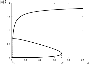
Figure 14: Numerical bifurcation diagram showing solutions of Eq. 3 for $\varepsilon=0.01$. Saddle-node bifurcations occur at $\lambda_{\ast}$ and $\lambda^{\ast}$.

Due to the singular dependence of $\lambda_{\ast}$ on the regularization parameter $\varepsilon$, an accurate numerical approximation is difficult to obtain for small values of $\varepsilon$. Using matched asymptotics, it was shown in [20] that $\lambda_{\ast}=\mathcal{O}(\varepsilon)$, with an expansion of the form

$$\lambda_{\ast}(\varepsilon)=\lambda_{\ast 0}\varepsilon+\lambda_{\ast 1}\varepsilon^{2}\ln\varepsilon+\lambda_{\ast 2}\varepsilon^{2}+\mathcal{O}(\varepsilon^{3}).$$

However, the coefficients $\lambda_{\ast i}$ remained undetermined there. Here, we confirm rigorously the structure of the above expansion, and we determine explicitly the values of the coefficients $\lambda_{\ast i}$ therein for $i=0,1$. Moreover, we indicate how higher-order coefficients may be found systematically, and we identify the source of the logarithmic (“switchback”) terms (in $\varepsilon$) in the expansion for $\lambda_{\ast}$; cf. Proposition 4.23 below.

Remark 4.19.

While a saddle-node bifurcation is equally observed in the bi-Laplacian case, recall Equation 2, Lindsay’s work [21] shows that the asymptotics of the associated $\lambda$-value $\lambda_{\ast}$ is far less singular in that case, allowing for a straightforward and explicit calculation of the corresponding coefficients.

To leading order, $\lambda_{\ast}$ equals the abovementioned critical value $\frac{3}{4}\varepsilon$, which corresponds to $\delta_{\ast}=\frac{2}{\sqrt{3}}$ in terms of $\delta$. That critical $\delta$-value was not covered in our discussion of region $\mathcal{R}_{1}$ in the previous section, as the argument applied in that region failed there; cf. Remark 4.12. Hence, a different argument is required for analysing the local dynamics in a neighborhood of the saddle-node bifurcation point at $\delta_{\ast}$.

In a first step, we consider the existence of singular solutions for varying $\delta$; in particular, the existence of type II-solutions in region $\mathcal{R}_{2}$ is guaranteed by the following

Lemma 4.20.

Let $\frac{1}{\sqrt{\lambda_{2}}}\leq\delta\leq\delta_{1}$, with $\delta_{1}<\frac{2}{\sqrt{3}}$. Then, a singular solution of type II exists if and only if $w_{1}=\mp\delta$ at $\xi_{1}=\mp 1$.

Proof 4.21.

In the original model, Equation 5, the “touchdown” solution of type II satisfies $w=\mp 1$ at $x=\mp 1$; cf. Definition 4.1. After the $w$-rescaling in Eq. 11, these boundary conditions are equivalent to $\tilde{w}=\mp\delta$ at $\xi=\mp 1$. The dynamics close to the boundary is naturally studied in chart $K_{1}$, which implies that $w_{1}=\mp\delta$ must hold at $\xi_{1}=\mp 1$; cf. Eq. 20a. For $\frac{1}{\sqrt{\lambda_{2}}}\leq\delta\leq\delta_{1}$, and in contrast to the solutions of type I considered in Section 4.1, the corresponding orbits can be fully studied in chart $K_{1}$, as they stay away from the critical manifold $\SS_{2}^{0}$ in $K_{2}$; recall Equation 36. The existence of a connecting orbit on the blow-up cylinder between $w_{1}=-\delta$ and $w_{1}=\delta$ then follows automatically; see the upper panel of Fig. 15.

Remark 4.22.

For $\delta=0$, the type II-solution constructed in Lemma 4.20 collapses onto the line $\{w_{1}=0\}$. That case, which requires further consideration, is studied in region $\mathcal{R}_{3}$; cf. Section 4.3. In fact, and as mentioned previously, both $\mathcal{R}_{2}$ and $\mathcal{R}_{3}$ are required to cover the green curve in Fig. 10.

Lemma 4.20 guarantees the existence of a type II-solution for every $\delta\in\big{[}\frac{1}{\sqrt{\lambda_{2}}},\delta_{1}\big{]}$, with $\delta_{1}<\delta_{\ast}$. For the same range of $\delta$, i.e., in the overlap between regions $\mathcal{R}_{1}$ and $\mathcal{R}_{2}$, Proposition 4.5 implies the local existence of type I-solutions. Hence, we can conclude that the boundary value problem {Eq. 13,Eq. 14} admits a pair of singular solutions for $\delta<\delta_{\ast}$; one of these is of type I, while the other is of type II. At $\delta=\delta_{\ast}$, the two singular solutions coalesce in a type II-solution. Finally, for $\delta>\delta_{\ast}$, no singular solution exists. The resulting three scenarios are illustrated in Fig. 15. In particular, we note that solutions of type I satisfy $w_{1}=\mp\frac{2}{\sqrt{3}}$ – or, equivalently, $w=\mp\frac{2}{\sqrt{3}\delta}$ in the original formulation – for $\xi_{1}=\mp 1$, while those of type II are characterized by $w_{1}=\mp\delta$ at $\xi_{1}=\mp 1$, as proven in Lemma 4.20; see again Fig. 15.

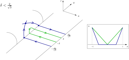
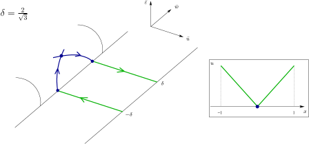
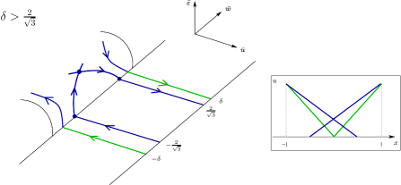
Figure 15: Saddle-node bifurcation in the singular limit of $\varepsilon=0$ in Equation 13 upon variation of $\delta$. In the respective insets, the corresponding singular solutions of types I (blue) and II (green) are shown. In particular, for $\delta>\frac{2}{\sqrt{3}}$, no solutions of types I or II exist.

The main result of this section is the following

Proposition 4.23.

There exists $\varepsilon_{0}>0$ sufficiently small such that in region $\mathcal{R}_{2}$, the boundary value problem {Eq. 13,Eq. 14} admits a unique branch of solutions for $\varepsilon\in(0,\varepsilon_{0})$. That branch consists of two sub-branches which limit on singular solutions of types I and II, respectively, as $\varepsilon\to 0$.

The two sub-branches meet in a saddle-node bifurcation point at $\lambda_{\ast}(\varepsilon)$, where two solutions exist for $\lambda>\lambda_{\ast}$ and $|\lambda-\lambda_{\ast}|$ small, whereas no solution exists for $\lambda<\lambda_{\ast}$. Moreover, for $\varepsilon\in(0,\varepsilon_{0})$, $\lambda_{\ast}$ has the asymptotic expansion

(76) $$\lambda_{\ast}(\varepsilon)=\frac{3}{4}\varepsilon-\bigg{(}\sqrt{\frac{3}{2}}+\frac{9}{8}\bigg{)}\varepsilon^{2}\ln\varepsilon+\mathcal{O}(\varepsilon^{2}).$$

The transition between regions $\mathcal{R}_{2}$ and $\mathcal{R}_{1}$ occurs as the branch of solutions limiting on solutions of type I connects to the branch already constructed in Proposition 4.5.

Proof 4.24.

The proof consists of two parts: we first consider a small neighborhood of $\delta_{\ast}=\frac{2}{\sqrt{3}}$ – i.e., of $\lambda=\frac{3}{4}\varepsilon$ – where the saddle-node bifurcation occurs. We define a suitable bifurcation equation, which describes the transition from solutions which limit on type I-solutions to those which limit on solutions of type II. Based on that equation, we infer the presence of the saddle-node bifurcation, and we calculate the expansion for the corresponding $\lambda$-value $\lambda_{\ast}$.

In a second step, we consider the branch of solutions that limit on type II-solutions for the remaining values of $\lambda$ in $\mathcal{R}_{2}$. Later, that branch will be shown to connect to solutions that are covered by region $\mathcal{R}_{3}$.

We begin by constructing the requisite bifurcation equation for the first step in our proof. Since $w\approx-\frac{2}{\sqrt{3}}$ and $\delta\approx\frac{2}{\sqrt{3}}$, we write

(77) $$w_{0}=-\frac{2}{\sqrt{3}}+\Delta w\quad\text{and}\quad\delta=\frac{2}{\sqrt{3}}+\Delta\delta.$$

in chart $K_{1}$.

Applying the shooting argument outlined in Section 2, we track the corresponding orbit from the initial manifold $\mathcal{V}_{1_{\varepsilon}}^{-}$ defined in Eq. 56 through $K_{1}$ and into the section $\Sigma_{1}^{\rm out}$; we denote that orbit by $\gamma_{1}^{-}$. In chart $K_{2}$, the point of intersection of the equivalent orbit $\gamma_{2}^{-}$ with the section $\Sigma_{2}^{\rm in}$ is then given by $(\sigma^{-1},w_{2}^{\rm in},\xi_{2}^{\rm in},\varepsilon)$, for appropriately defined $w_{2}^{\rm in}$ and $\xi_{2}^{\rm in}$.

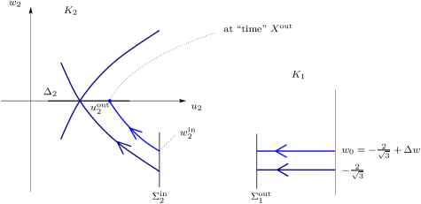
Figure 16: Sketch of the shooting argument underlying the proof of Proposition 4.23.

Next, we consider the evolution of the orbit $\gamma_{2}^{-}$ through $K_{2}$. Let $X^{\rm out}$ denote the “time” at which $\gamma_{2}^{-}$ reaches the hyperplane $\Delta_{2}=\{w_{2}=0\}$, viz. $w_{2}(X^{\rm out})=0$. (By symmetry, it then follows that the reflection $\gamma_{2}^{+}$ of $\gamma_{2}^{-}$ under the map $(u_{2},w_{2},\xi_{2},r_{2})\mapsto(u_{2},-w_{2},-\xi_{2},r_{2})$ will satisfy the boundary condition at $\mathcal{V}_{1_{\varepsilon}}^{+}$, with $w_{0}=\frac{2}{\sqrt{3}}-\Delta w$, after transformation to $K_{1}$.) Clearly, $X^{\rm out}$ depends on $w_{2}^{\rm in}$ and, in particular, on $\Delta w$, i.e., on the initial deviation of the orbit from its singular limit $\Gamma_{1}^{-}$ in chart $K_{1}$.

As per our shooting argument, we need to impose the constraint that $\xi_{2}(X^{\rm out})=0$. Dividing Equation 26c by Equation 26a and recalling that $r_{2}=\varepsilon$ in chart $K_{2}$, we find $\frac{\mathrm{d}\xi_{2}}{\mathrm{d}u_{2}}=\frac{\delta\varepsilon}{w_{2}}$ and, therefore,

(78) $$\xi_{2}(u_{2})=\xi_{2}^{\rm in}+\delta\varepsilon\int_{u_{2}^{\rm in}}^{u_{2}^{\rm out}}\frac{1}{w_{2}(u_{2})}\,\mathrm{d}u_{2}.$$

Here, $u_{2}^{\rm in}=\sigma^{-1}$ as in the definition of $\Sigma_{2}^{\rm in}$ in Eq. 28, while $u_{2}^{\rm out}$ denotes the value of $u_{2}$ such that $w_{2}(u_{2}^{\rm out})=0$; cf. again Fig. 16.

The sought-after bifurcation equation now corresponds to a relation between $\Delta w$, $\varepsilon$, and $\delta$ that is satisfied for any solution to the boundary value problem {Eq. 13,Eq. 14} close to the saddle-node bifurcation in Equation 13. To derive such a relation, we must first approximate $u_{2}^{\rm out}$: recalling the explicit expression for $w_{1}(\varepsilon_{1})$ on $\gamma_{1}^{-}$, as given in Eq. 58, substituting the Ansatz made in Equation 77, and rewriting the result in the coordinates of chart $K_{2}$, we find

(79) $$w_{2}(u_{2})=-\sqrt{\Big{(}-\frac{2}{\sqrt{3}}+\Delta w\Big{)}^{2}+2\Big{(}\varepsilon-\frac{1}{u_{2}}\Big{)}-\frac{2}{3}\Big{(}\varepsilon^{3}-\frac{1}{u_{2}^{3}}\Big{)}}$$

on $\gamma_{2}^{-}$. Next, we write $u_{2}^{\rm out}=1+\Delta u$ in Eq. 79, where $\Delta u$ is assumed to be sufficiently small due to the fact that we stay close to the equilibrium at $(u_{2},w_{2})=(1,0)$ in $K_{2}$. Then, we solve the resulting expression for $\Delta u$ to find three roots; two of these are complex conjugates, and are hence irrelevant due to the real nature of our problem. Expanding the third root, which is real irrespective of the value of $\Delta w$, in a series with respect to $\Delta w$ and $\varepsilon$, we find

(80) $$u_{2}^{\rm out}=1+\frac{13\sqrt{3}}{9}\Delta w-\frac{13}{6}\varepsilon+\mathcal{O}(2),$$

to first order in $\Delta w$ and $\varepsilon$.

It remains to determine the leading-order asymptotics of the integral in Eq. 78. To that end, we expand the integrand therein as

(81) $$\frac{1}{w_{2}(u_{2})}=-\sqrt{\frac{3u_{2}^{3}}{2(u_{2}-1)^{2}(2u_{2}+1)}}+\mathcal{O}(\Delta w,\varepsilon),$$

which can be shown to be sufficient to the order of accuracy considered here. (The inclusion of higher-order terms in Eq. 78 would yield a refined bifurcation equation, and would hence allow us to take the expansion for $\lambda_{\ast}$ in Eq. 76 to higher order in $\varepsilon$.)

Combining Eq. 81 and Eq. 80 and noting that $u_{2}^{\rm in}$ only enters through higher-order terms in $\Delta w$, which are neglected here, we finally obtain the expansion

(82) $$\int_{u_{2}^{\rm in}}^{u_{2}^{\rm out}}\frac{1}{w_{2}(u_{2})}\,\mathrm{d}u_{2}=-\frac{\sqrt{2}}{2}\ln\Delta w+C+\mathcal{O}(\Delta w)$$

where $C$ is a computable constant. (The above expansion reflects the fact that, as $\Delta w\to 0$, i.e., as the point $(\sigma^{-1},w_{2}^{\rm in},\xi_{2}^{\rm in},\varepsilon)$ tends to the stable manifold $\mathcal{W}_{2}^{\rm s}(Q_{2})$, the “time” required for reaching $\Delta_{2}$ tends to infinity. Moreover, it is consistent with the observation that expansions of solutions passing close to equilibria or slow manifolds of saddle type frequently involve logarithmic terms.)

Next, we substitute $\xi_{2}^{\rm in}(=\xi_{1}^{\rm out})=-1-\frac{\delta}{w_{0}}+\frac{\delta}{w_{0}^{3}}\varepsilon\ln\varepsilon+\mathcal{O}(\varepsilon)$ from Eq. 59 into Eq. 82 to obtain

(83) $$\xi_{2}(u_{2}^{\rm out})=-1-\frac{\delta}{w_{0}}-\frac{\sqrt{2}}{2}\delta\varepsilon\ln\Delta w+\frac{\delta}{w_{0}^{3}}\varepsilon\ln\varepsilon+\mathcal{O}(\varepsilon)\stackrel{{\scriptstyle!}}{{=}}0.$$

Shifting $w_{0}$ and $\delta$ by $\Delta w$ and $\Delta\delta$, cf. Eq. 77, and solving Eq. 83 for $\Delta\delta$, we obtain the following bifurcation equation in $(\Delta w,\Delta\delta,\varepsilon)$:

(84) $$\Delta\delta=-\Delta w+\frac{2\sqrt{2}}{3}\varepsilon\ln\Delta w+\frac{\sqrt{3}}{2}\varepsilon\ln\varepsilon+\mathcal{O}(\varepsilon).$$

The last step consists in finding the $\Delta w$-value $\Delta w_{\ast}$ at which the bifurcation equation in Eq. 84 attains its minimum, corresponding to the approximate location of the saddle-node bifurcation in Equation 13, and in reverting to the original scalings. To that aim, we differentiate Equation 84 and solve $\frac{\mathrm{d}\Delta\delta}{\mathrm{d}\Delta w}=0$ to leading order, which yields $\Delta w_{\ast}=\frac{2\sqrt{2}}{3}\varepsilon$; see Fig. 17.

Substituting into Eq. 84, we obtain the corresponding value of $\Delta\delta_{\ast}$, which implies $\lambda_{\ast}=\frac{\varepsilon}{\delta_{\ast}^{2}}=\varepsilon\big{(}\frac{2}{\sqrt{3}}+\Delta\delta_{\ast}\big{)}^{-2}$ by Equation 77. Hence, we find the desired asymptotic expansion for $\lambda_{\ast}$, viz.

(85) $$\lambda_{\ast}(\varepsilon)=\frac{3}{4}\varepsilon-\bigg{(}\sqrt{\frac{3}{2}}+\frac{9}{8}\bigg{)}\varepsilon^{2}\ln\varepsilon+\mathcal{O}(\varepsilon^{2}),$$

as claimed. Finally, since

$$\frac{\mathrm{d}^{2}\Delta\delta}{\mathrm{d}(\Delta w)^{2}}\bigg{|}_{\Delta w=\Delta w_{\ast}}=-\frac{2\sqrt{2}}{3}\frac{\varepsilon}{(\Delta w_{\ast})^{2}}$$

is negative, the function $\Delta\delta(\Delta w)$ is locally concave, which implies that the unfolding of solutions to Equation 13 for $|\lambda-\lambda_{\ast}|$ small is as given in the statement of the proposition; see 17(a). In particular, the branch of solutions which limits on solutions of type I overlaps with the one contained in region $\mathcal{R}_{1}$, as $\delta_{1}$ can be chosen arbitrarily close to $\frac{2}{\sqrt{3}}$ in the statement of Proposition 4.5.

The last part of the proof concerns the existence of solutions to the boundary value problem {Eq. 13,Eq. 14} which limit on type II-solutions as $\varepsilon\to 0$ for the remaining values of $\lambda$ in $\mathcal{R}_{2}$, i.e., for $\delta\in\big{(}\frac{1}{\sqrt{\lambda_{2}}},\delta_{1}\big{)}$. The existence of singular solutions of type II in that range is ensured by Lemma 4.20. In the singular limit, i.e., for $\varepsilon=0$, we have transversality at $\xi_{1}=0$ with respect to variation of $w_{1}$ at $\xi_{1}=\mp 1$ around $\mp\delta$. Hence, the corresponding singular solutions perturb to solutions of the boundary value problem {Eq. 13,Eq. 14} for $0<\varepsilon\ll 1$, which completes the proof.

Remark 4.25.

The branch of solutions derived in the last part of the proof is still described by the bifurcation equation in Eq. 84, the difference being that the $\varepsilon\ln\Delta w$-term is now regular, i.e., $\mathcal{O}(\varepsilon)$, due to $\Delta w=\mathcal{O}(1)$. The above proof also implies that $\Delta\delta$ must be larger than $\mathcal{O}(\varepsilon)$; in fact, Lindsay’s work [20] shows that $\Delta\delta=\mathcal{O}(\varepsilon\ln\varepsilon)$.

Remark 4.26.

The presence of an $\varepsilon\ln\varepsilon$-term in the bifurcation equation Eq. 84 implies that the convergence to the singular limit of $\varepsilon=0$ cannot be smooth in $\varepsilon$; rather, it will be regular in $(\varepsilon,\ln\varepsilon)$. A similar situation was encountered in Proposition 4.5 above, where the presence of logarithmic switchback terms in $\varepsilon$ was observed; recall Section 4.1.5. Here, we emphasize that the source of these terms in Eq. 84 is two-fold: in addition to switchback due to a resonance in chart $K_{1}$, logarithmic terms are also introduced through the passage of the flow past the saddle point at $(1,0)$ in $K_{2}$, as is evident from the $\varepsilon\ln\Delta w$-term in Equation 82. In particular, both contributions manifest in the expansion for $\lambda_{\ast}(\varepsilon)$ in Equation 85.

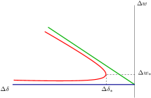
(a) Local view.

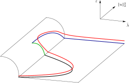
(b) Global view.

Figure 17: Illustration of the saddle-node bifurcation at $\lambda_{\ast}$ in Equation 13. The red curve corresponds to the case of $\varepsilon\neq 0$, while the singular limit of $\varepsilon=0$ is represented in blue (type I), green (type II), and black (type III). The point of intersection of the green and blue curves corresponds to the critical $\delta$-value $\delta_{\ast}$; a small neighborhood of that point where the transition between these two curves occurs is considered in the first part of Proposition 4.23, while the remainder of the green curve – up to an arbitrarily small, but fixed distance from the intersection with the black curve – is studied in the second part of Proposition 4.23. Finally, the transition between the green and black curves is described in Section 4.3 below.

The asymptotic expansion for $\lambda_{\ast}$ in Eq. 76 shows excellent agreement with numerical values that were obtained using the continuation software package AUTO [2]; see Fig. 18. In particular, the distance between the two curves is $\mathcal{O}(\varepsilon^{2})$, i.e., of higher order in $\varepsilon$, as postulated.

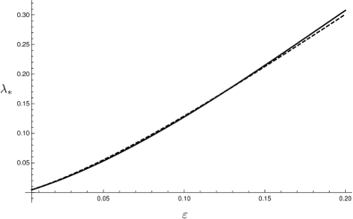
Figure 18: Comparison between the asymptotic expansion for $\lambda_{\ast}(\varepsilon)$ in Eq. 76 (solid curve) and numerical values obtained with AUTO (dashed curve).

4.3 Region $\mathcal{R}_{3}$

It remains to analyse region $\mathcal{R}_{3}$, which contains the branch of solutions in the bifurcation diagram that perturb from type III-solutions, corresponding to the non-regularized problem

(86) $$u^{\prime\prime}=\frac{\lambda}{u^{2}},\qquad\text{ for }x\in[-1,1],\text{ with }u=1\text{ when }x=\mp 1.$$

By Definition 4.1, solutions of type III differ from those of types I and II, in that they do not exhibit touchdown phenomena. Regularization affects them only weakly, i.e., in a regular fashion, with the effect becoming slightly more pronounced as $\lambda\to 0$; cf. Fig. 19. Thus, most of the solutions contained in region $\mathcal{R}_{3}$ perturb from $\mathcal{B}_{3}$ in a regular way, and are hence easy to obtain. The limit of $\lambda\to 0$, i.e., the transition from $\mathcal{R}_{3}$ to $\mathcal{R}_{2}$, needs to be treated more carefully.

Remark 4.27.

It is easy to see that Equation 86 – or, rather, the corresponding first-order system – is Hamiltonian; the level curves of the associated Hamiltonian are given precisely by the singular solutions in panel (b) of Fig. 19.

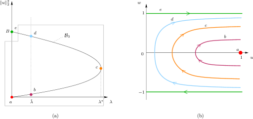
Figure 19: (a) Covering of the curve $\mathcal{B}_{3}$ by region $\mathcal{R}_{3}$ for $\varepsilon>0$; (b) the corresponding singular solutions in the original $(u,w)$-space. The green solution is of type II, and corresponds to the limit as $\lambda\to 0$. Recall that, for $\varepsilon\to 0$, $\mathcal{R}_{3}$ approaches the line $\{\lambda=0\}$ near the point $B$. Singular solutions corresponding to $\lambda>0$ are of type III and do not exhibit touchdown phenomena. The orange solution realized at the fold point $\lambda=\lambda^{\ast}$ is the one where the two parts of the curve $\mathcal{B}_{3}$ meet.

Type III-solutions are contained in the curve $\mathcal{B}_{3}$ in the limit of $\delta=0$; see Fig. 11. That limit was not covered in region $\mathcal{R}_{2}$, as the approach used there required the assumption that $\delta\geq\frac{1}{\sqrt{\lambda_{2}}}$. The limit as $\delta\to 0$, however, results in singular dynamics in chart $K_{1}$, as the type II-solution (green) – corresponding to $w_{1}=\mp\delta$ at $\xi_{1}=\mp 1$ – collapses onto the line

(87) $$\mathcal{M}_{1}^{0}:=\big{\{}(r_{1},0,\xi_{1},0)\,\big{|}\,r_{1}\in\mathbb{R}^{+},\ \xi_{1}\in\mathbb{R}\big{\}};$$

see Fig. 5 and the upper panel of Fig. 15. Clearly, $\mathcal{M}_{1}^{0}$ constitutes a line of non-hyperbolic equilibria for Equation 24 which corresponds to the manifold $\mathcal{M}^{0}$ in Eq. 10, after blow-down. The singular nature of $\mathcal{M}_{1}^{0}$ is related to the rescaling of $w$ introduced in Eq. 11. That rescaling, which corresponded to a “zooming out”, turned out to be particularly useful for our analysis in regions $\mathcal{R}_{1}$ and $\mathcal{R}_{2}$. However, it cannot provide a good description of region $\mathcal{R}_{3}$. To study the dynamics in $\mathcal{R}_{3}$, we would have to perform another blow-up involving $\delta$, $w_{1}$, and $\varepsilon_{1}$ in chart $K_{1}$ in order to basically undo the $w$-rescaling in Eq. 11. It is much simpler to consider the $\delta$-range covered by $\mathcal{R}_{3}$ by returning to the original system without any rescaling of $w$; cf. Equation 7.

The main result of this section is the following

Proposition 4.28.

There exists $\varepsilon_{0}>0$ sufficiently small such that in region $\mathcal{R}_{3}$, the boundary value problem {Eq. 7,Eq. 8} admits a unique branch of solutions for $\varepsilon\in(0,\varepsilon_{0})$. Outside of a fixed neighborhood of the point $B$, that branch converges smoothly as $\varepsilon\to 0$ to the curve $\mathcal{B}_{3}$ along which solutions of the non-regularized boundary value problem, Equation 86, exist. In the $\varepsilon$-dependent region overlapping with $\mathcal{R}_{2}$, the branch of solutions limiting on solutions of type II described in Proposition 4.23 is recovered. There, the transition from solutions that limit on type-III solutions to those limiting on singular solutions of type II occurs.

Proof 4.29.

We recall the original first-order system, Equation 7:

$$u^{\prime} =u^{4}w,$$

$$w^{\prime} =\lambda(u^{2}-\varepsilon^{2}),$$

$$\xi^{\prime} =u^{4},$$

$$\varepsilon^{\prime} =0;$$

given Equation 12, we write $\varepsilon=\delta^{2}\lambda$ and obtain the equivalent system

(88a) $$u^{\prime} =u^{4}w,$$

(88b) $$w^{\prime} =\lambda(u^{2}-\delta^{4}\lambda^{2}),$$

(88c) $$\xi^{\prime} =u^{4},$$

(88d) $$\delta^{\prime} =0.$$

Here, the parameter $\delta$ plays the role of the small perturbation parameter, with the $\delta$-range corresponding to region $\mathcal{R}_{3}$ given by

$$\delta\in\Big{[}0,\frac{1}{\sqrt{\lambda_{3}}}\Big{]};$$

cf. Eq. 31. In summary, it is hence more convenient to consider $\lambda$ and $\delta$, rather than $\lambda$ and $\varepsilon$, as the relevant parameters in this regime.

For $\delta=0$ and $\lambda>0$, the projection of the flow of Equation 88 is as illustrated in Fig. 4. In region $\mathcal{R}_{3}$, however, we are also interested in covering a small neighborhood of $\lambda=0$, which again gives the singular dynamics shown in Fig. 5. In $(u,w)$-space, the singular solution found for $\lambda=0$ consists of $[0,1]\times\{-1\}$ and $[0,1]\times\{1\}$, i.e., it approaches the degenerate line of equilibria for Eq. 88 at $\{(0,w)\}$ under the forward and backward flow in $x$, respectively; see Fig. 20.

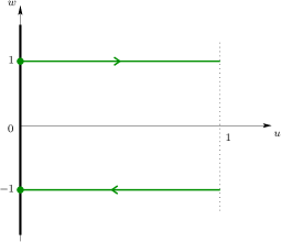
Figure 20: Singular solution of Equation 88 for $(\delta,\lambda)=(0,0)$ in $(u,w)$-space. That solution, which is of type II, cf. Fig. 8, is shown in green. The solid black line represents the degenerate line of equilibria at $\{(0,w)\}$.

To analyze the dynamics close to that line, we have to introduce a blow-up of $(u,\lambda)=(0,0)$. As the blow-up involves $\lambda$, we append the trivial equation $\lambda^{\prime}=0$ to Eq. 88:

(89a) $$u^{\prime} =u^{4}w,$$

(89b) $$w^{\prime} =\lambda(u^{2}-\delta^{4}\lambda^{2}),$$

(89c) $$\xi^{\prime} =u^{4},$$

(89d) $$\lambda^{\prime} =0,$$

(89e) $$\delta^{\prime} =0.$$

The requisite blow-up transformation is then given by

(90) $$u=\bar{r}\bar{u}\qquad\text{and}\qquad\lambda=\bar{r}\bar{\lambda},$$

where $(\bar{u},\bar{\lambda})\in S^{1}$, i.e., $\bar{u}^{2}+\bar{\lambda}^{2}=1$, and $\bar{r}\in[0,r_{0})$, with $r_{0}>0$. We denote the chart corresponding to $\bar{u}=1$ by $\kappa_{1}$. The analysis in that chart turns out to be sufficient for proving Proposition 4.28. In chart $\kappa_{1}$, the blow-up transformation in Eq. 90 reads

(91) $$u=r_{1}\qquad\text{and}\qquad\lambda=r_{1}\lambda_{1}.$$

which gives

(92a) $$r_{1}^{\prime} =r_{1}w,$$

(92b) $$w^{\prime} =\lambda_{1}(1-\delta^{4}\lambda_{1}^{2}),$$

(92c) $$\xi^{\prime} =r_{1},$$

(92d) $$\lambda_{1}^{\prime} =-\lambda_{1}w,$$

(92e) $$\delta^{\prime} =0$$

for Equation 89; here, $\delta$ is the small (regular) perturbation parameter. For any $\lambda\in[0,1]$, the existence of solutions to Eq. 92 can be studied via the symmetric shooting argument outlined in Section 2. To that end, we define a set of initial conditions at $(r_{1},\xi)=(1,-1)$, as follows:

(93) $$\mathcal{V}_{\lambda}=\big{\{}(1,w_{0},-1,\lambda,\delta)\,\big{|}\,w_{0}\in I\big{\}},$$

where $I$ is a neighborhood of $w=-1$. We remark that the initial value $\lambda$ for $\lambda_{1}$ follows from $\lambda=r_{1}\lambda_{1}$, cf. Eq. 91, as $r_{1}=1$ initially. Next, we introduce $w$ as the independent variable in Eq. 92, whence

(94a) $$\frac{{\rm d}r_{1}}{{\rm d}w} =\frac{r_{1}w}{\lambda_{1}(1-\delta^{4}\lambda_{1}^{2})},$$

(94b) $$\frac{{\rm d}\xi}{{\rm d}w} =\frac{r_{1}}{\lambda_{1}(1-\delta^{4}\lambda_{1}^{2})},$$

(94c) $$\frac{{\rm d}\lambda_{1}}{{\rm d}w} =-\frac{w}{1-\delta^{4}\lambda_{1}^{2}},$$

(94d) $$\frac{{\rm d}\delta}{{\rm d}w} =0,$$

with initial conditions

(95) $$r_{1}(w_{0})=1,\quad\xi(w_{0})=-1,\quad\lambda_{1}(w_{0})=\lambda,\quad\text{and}\quad\delta(w_{0})=0.$$

We track $\mathcal{V}_{\lambda}$ under the flow of Eq. 94 up to the hyperplane $\{w=0\}$; see Fig. 21. There, we obtain a point $(r_{1}^{\rm out},0,\xi^{\rm out},\lambda_{1}^{\rm out},\delta)$ in $(r_{1},w,\xi,\lambda_{1},\delta)$-space. Our shooting argument implies that we have to solve the equation

(96) $$\xi^{\rm out}(w_{0},\lambda,\delta)=0.$$

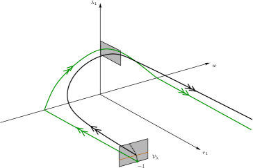
Figure 21: Dynamics of Equation 92 in $(r_{1},w,\lambda_{1})$-space. The gray section at $r_{1}=1$ corresponds to $\mathcal{V}_{\lambda}$, cf. Eq. 93, which is flown forward to $\{w=0\}$. The green orbit represents the singular solution for $\lambda=0$, i.e., a singular solution of type II, which satisfies $w=-1$ at $\xi=-1$. The black orbit corresponds to a solution of Eq. 92 with initial conditions in $\mathcal{V}_{\lambda}$ for a fixed value of $\lambda>0$ and $\delta=0$, which is a solution of type III. The dashed curve contained in $\mathcal{V}_{\lambda}$ corresponds to the set $\{w_{0}=w_{0}(\lambda)\}$ that solves Equation 98. That set is defined by Equation 99 for $\delta=0$. The orange line indicates a section through $\mathcal{V}_{\lambda}$ for fixed $\lambda>0$.

At this point, we split $\mathcal{R}_{3}$ into two subregions in which we apply separate arguments to prove the existence of a unique branch of solutions, as claimed in the statement of the proposition. For $\lambda\geq\tilde{\lambda}$, with $\tilde{\lambda}$ fixed and positive, and $\delta=0$, Equation 94 can be solved explicitly subject to Eq. 95; moreover, a solution $w_{0}=w_{0}(\lambda)$ of Equation 96 can be proven to exist for $\lambda\leq\lambda^{\ast}$. At $\lambda=\lambda^{\ast}$, transversality breaks down, as Equation 96 does not admit a solution for $\lambda>\lambda^{\ast}$. The corresponding singular solutions are of type III; cf. Definition 4.1. Due to the regularity of Eq. 96 with respect to $\delta$, these solutions perturb in a regular fashion to solutions of {Eq. 94,Eq. 95} for $\delta$ positive and small; in particular, we consider $\delta\leq\frac{1}{\sqrt{\lambda_{3}}}$ with $\lambda_{3}$ large, in accordance with Eq. 31. For $\lambda$ close to $\lambda^{\ast}$, individual solutions do not perturb regularly; however, the structurally stable saddle-node bifurcation at $\lambda^{\ast}$ as a whole will persist as a regular perturbation, giving rise to a slightly perturbed value $\lambda^{\ast}(\delta)$ for the perturbed saddle-node point. Since the resulting asymptotics of $\lambda^{\ast}(\delta)$ is not our main concern, we do not consider it further here.

The second subregion of $\mathcal{R}_{3}$, which includes the overlap with region $\mathcal{R}_{2}$, corresponds to a small neighborhood of $(\lambda,\delta)=(0,0)$ that is given by

(97) $$(\lambda,\delta)\in\big{[}0,\tilde{\lambda}\big{]}\times\Big{[}0,\frac{1}{\sqrt{\lambda_{3}}}\Big{]}.$$

To study the branch of solutions in this subregion, we solve Equation 94 with initial conditions as in Eq. 95 by expanding around $(w_{0},\lambda,\delta)=(-1,0,0)$, and by making use of the fact that the equations can be solved explicitly for $\delta=0$. Linearizing Equation 96 around $\delta=0$, we obtain a regular perturbation problem in $\delta$ for $\xi^{\rm out}$, which gives the following expanded form of Equation 96, up to higher-order terms in $(w_{0},\lambda,\delta)$:

(98) $$w_{0}+1-(4+3w_{0})\lambda\ln\lambda+\frac{1}{288}(1+w_{0})\delta^{8}\ln\lambda=0.$$

Equation 98 again contains logarithmic terms due to resonance between the eigenvalues $-1$, $0$ (double), and $1$ of the linearization of Equation 92 about the steady state at $(0,-1,-1,0)$ in chart $\kappa_{1}$. These terms arise in the passage of orbits through a neighborhood of $\{r_{1}=0\}$, as was observed in chart $K_{1}$; see Section 4.1.5. Solving Equation 98 for $w_{0}$ gives

(99) $$w_{0}=-1+\lambda\ln\lambda+C(\delta)\lambda+\mathcal{O}\big{[}\lambda^{2}(\ln\lambda)^{2}\big{]}$$

with $C(\delta)=\mathcal{O}(\delta^{8})$, which is regular in $\delta$, as expected. We note that, for $\lambda=0$, Eq. 98 reduces to the trivial equation $w_{0}+1=0$, which is solved by $w_{0}=-1$, irrespective of $\delta$. The resulting singular solutions are type II-solutions, which are shown as the part of the green curve in the blown-up bifurcation diagram in Fig. 10 that corresponds to $\bar{\varepsilon}$ small. In line with these observations, Equation 98 is identical to Equation 83 up to terms of order $\mathcal{O}(\delta^{2}\lambda)$ after the rescaling of $w$ in Eq. 11. For $\delta=0$ and $\lambda>0$, on the other hand, we match with the branch obtained in the part of region $\mathcal{R}_{3}$ that corresponds to $\lambda\geq\tilde{\lambda}$.

The results obtained in the above two subregions prove the existence and uniqueness of a curve of solutions to the boundary value problem {Eq. 13,Eq. 14} in $\mathcal{R}_{3}$, as stated in Proposition 4.28. It remains to consider the overlap between regions $\mathcal{R}_{3}$ and $\mathcal{R}_{2}$: in $(\lambda,\delta)$-space, $\mathcal{R}_{3}$ corresponds to

(100) $$[0,1]\times\bigg{[}0,\frac{1}{\sqrt{\lambda_{3}}}\bigg{]}\setminus[0,\varepsilon\lambda_{3}]\times\bigg{[}\frac{1}{\sqrt{\lambda_{2}}},\frac{1}{\sqrt{\lambda_{3}}}\bigg{]},$$

while $\mathcal{R}_{2}$ covers the area

(101) $$[0,\varepsilon\lambda_{2}]\times\bigg{[}\frac{1}{\sqrt{\lambda_{2}}},\delta_{1}\bigg{]},$$

where $\delta_{1}<\frac{2}{\sqrt{3}}$ is defined as in Proposition 4.5. Hence, in $(\lambda,\delta)$-space, regions $\mathcal{R}_{3}$ and $\mathcal{R}_{2}$ overlap in the rectangle

(102) $$[\varepsilon\lambda_{3},\varepsilon\lambda_{2}]\times\bigg{[}\frac{1}{\sqrt{\lambda_{2}}},\frac{1}{\sqrt{\lambda_{3}}}\bigg{]},$$

see Fig. 22, which is the area where the transition between the two regions occurs. This concludes the proof of Proposition 4.28.

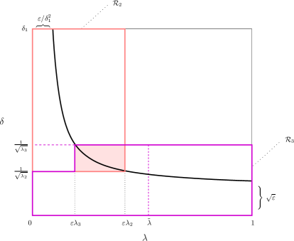
Figure 22: Regions $\mathcal{R}_{2}$ (pink) and $\mathcal{R}_{3}$ (magenta) in $(\lambda,\delta)$-parameter space; cf. Eq. 101 and Eq. 100, respectively. The dashed vertical magenta line at $\lambda=\tilde{\lambda}$ delimits the two subregions considered in the proof of Proposition 4.28. The dashed horizontal magenta line at $\delta=\frac{1}{\sqrt{\lambda_{3}}}$ indicates that the argument employed in the second part of the proof of Proposition 4.28 is valid in the entire rectangle defined in Eq. 97, where we note that region $\mathcal{R}_{3}$ excludes the rectangle $[0,\varepsilon\lambda_{3}]\times\big{[}\frac{1}{\sqrt{\lambda_{2}}},\frac{1}{\sqrt{\lambda_{3}}}\big{]}$ by construction; cf. Eq. 31. Regions $\mathcal{R}_{2}$ and $\mathcal{R}_{3}$ overlap in the shaded rectangle (light pink) given by Eq. 102. The black curve corresponds to $\delta^{2}\lambda=\varepsilon$, for given $0<\varepsilon\ll 1$.

The last step in the proof of Theorem 1.2 consists in proving Equation 4.

Proposition 4.30.

For $\varepsilon\in(0,\varepsilon_{0})$, with $\varepsilon_{0}>0$ sufficiently small, the upper branch of solutions in Fig. 3 has the expansion stated in Equation 4.

Proof 4.31.

We first express $\|u\|_{2}^{2}$, with $u$ being the original variable considered in Equation 3, in terms of our shifted variable $\tilde{u}$, as defined in Equation 6:

(103) $$\|u\|_{2}^{2}=2-2\|\tilde{u}\|_{1}+\|\tilde{u}\|_{2}^{2}.$$

(While we had omitted the tilde in our notation following Eq. 6, we now include it again for the sake of clarity.) Due to the symmetry of the boundary value problem {Eq. 13,Eq. 14}, we can focus our attention on the interval $[-1,0]$; correspondingly, we split the integrals occurring in Equation 103 into two parts, which are divided by the section $\Sigma_{1}^{\rm out}$ defined in Eq. 27b. Since $\xi_{1}^{\rm out}=\xi_{2}^{\rm in}$, that split implies $[-1,0]=[-1,\xi_{1}^{\rm out}]\cup[\xi_{2}^{\rm in},0]$ and, hence, that these integrals can be investigated separately in charts $K_{1}$ and $K_{2}$:

(104a) $$\begin{split}\|\tilde{u}\|_{1}&=\int_{-1}^{1}\tilde{u}(\xi)\,\mathrm{d}\xi=2\int_{-1}^{0}\tilde{u}(\xi)\,\mathrm{d}\xi\\ &=2\Bigg{(}\int_{-1}^{\xi_{1}^{\mathrm{out}}}r_{1}(\xi_{1})\,\mathrm{d}\xi_{1}+\int_{\xi_{2}^{\mathrm{in}}}^{0}r_{2}(\xi_{2})u_{2}(\xi_{2})\,\mathrm{d}\xi_{2}\Bigg{)}\quad\text{and}\end{split}$$

(104b) $$\begin{split}\|\tilde{u}\|_{2}^{2}&=\int_{-1}^{1}\tilde{u}^{2}(\xi)\,\mathrm{d}\xi=2\int_{-1}^{0}\tilde{u}^{2}(\xi)\,\mathrm{d}\xi\\ &=2\Bigg{(}\int_{-1}^{\xi_{1}^{\mathrm{out}}}r_{1}^{2}(\xi_{1})\,\mathrm{d}\xi_{1}+\int_{\xi_{2}^{\mathrm{in}}}^{0}(r_{2}(\xi_{2})u_{2}(\xi_{2}))^{2}\,\mathrm{d}\xi_{2}\Bigg{)},\end{split}$$

where $\xi_{1}^{\mathrm{out}}(=\xi_{1}^{{\rm out}-})$ is approximated as in Equation 59. Dividing Equation 24c by Equation 24a and using Eq. 58, where we recall that $\varepsilon_{1}=\frac{\varepsilon}{r_{1}}$, we can rewrite the $\xi_{1}$-integrals in Equation 104 as integrals in $r_{1}$, with $r_{1}\in[1,\frac{\varepsilon}{\sigma}]$. Expanding the resulting integrands for small $\varepsilon$ and evaluating the integrals to the corresponding order, we obtain

$$\int_{-1}^{\xi_{1}^{\mathrm{out}}}r_{1}(\xi_{1})\,\mathrm{d}\xi_{1}=\frac{\sqrt{3}}{2}\sqrt{\frac{\varepsilon}{\lambda}}+\mathcal{O}(\varepsilon^{\frac{3}{2}})\quad\text{and}\quad\int_{-1}^{\xi_{1}^{\mathrm{out}}}r_{1}^{2}(\xi_{1})\,\mathrm{d}\xi_{1}=\frac{\sqrt{3}}{3}\sqrt{\frac{\varepsilon}{\lambda}}+\mathcal{O}(\varepsilon^{2}).$$

As for the integrals in $\xi_{2}$, we recall from Eq. 20b that $r_{2}=\varepsilon$ in chart $K_{2}$. Moreover, given the fast-slow structure of Equation 26, $u_{2}$ can be expressed as the sum of a slow and a fast component,

$$u_{2}(\xi_{2})=1+\check{u}_{2}(\tfrac{\xi_{2}}{\varepsilon});$$

by the definition of the slow manifold $\SS_{2}^{\varepsilon}$ in Lemma 4.8, the slow contribution is given by $u_{2}(\xi_{2})\sim 1$, while the fast contribution $\check{u}_{2}$ is obtained from the corresponding stable foliation $\mathcal{F}_{2}^{\rm s}(\SS_{2}^{\varepsilon})$. In particular, the latter yields higher-order terms in the $\xi_{2}$-integrals in Eq. 104, which implies

$$\int_{\xi_{2}^{\mathrm{in}}}^{0}r_{2}(\xi_{2})u_{2}(\xi_{2})\,\mathrm{d}\xi_{2}=2\varepsilon+\mathcal{O}(\varepsilon^{\frac{3}{2}}\ln\varepsilon)\quad\text{and}\quad\int_{\xi_{2}^{\mathrm{in}}}^{0}\big{(}r_{2}(\xi_{2})u_{2}(\xi_{2})\big{)}^{2}\,\mathrm{d}\xi_{2}=\mathcal{O}(\varepsilon^{2}).$$

Combining these estimates into Equation 103, we obtain

$$\|u\|_{2}^{2} =2-2\bigg{(}\frac{\sqrt{3}}{2}\sqrt{\frac{\varepsilon}{\lambda}}+2\varepsilon+\mathcal{O}(\varepsilon^{\frac{3}{2}}\ln\varepsilon)\bigg{)}+\frac{\sqrt{3}}{3}\sqrt{\frac{\varepsilon}{\lambda}}+\mathcal{O}(\varepsilon^{2})$$

$$=2\bigg{(}1-\frac{\sqrt{3}}{3}\sqrt{\frac{\varepsilon}{\lambda}}-2\varepsilon+\mathcal{O}(\varepsilon^{\frac{3}{2}}\ln\varepsilon)\bigg{)},$$

which is precisely Equation 4.

Theorem 1.2 is hence proven.

Remark 4.32.

Our analysis suggests that the expansion for the upper solution branch in Equation 4 is still valid up to an $\mathcal{O}(\varepsilon)$-neighborhood of the fold point at $\lambda_{\ast}(\varepsilon)$; that expansion hence provides a good approximation close to the point where the middle and upper branches in Fig. 3 meet. Differentiating Equation 4 with respect to $\lambda$, evaluating the derivative at $\lambda=\lambda_{\ast}(\varepsilon)$, as given in Equation 76, and expanding for $\varepsilon$ small, we obtain

(105) $$\frac{\mathrm{d}\|u\|_{2}^{2}}{\rm{d}\lambda}\bigg{|}_{\lambda=\lambda_{\ast}(\varepsilon)}=\frac{8}{9\varepsilon}+\frac{2}{9}\big{(}9+4\sqrt{6}\big{)}\ln\varepsilon+\frac{5}{36}\big{(}59+24\sqrt{6}\big{)}\varepsilon(\ln\varepsilon)^{2}+\mathcal{O}(\varepsilon^{2}),$$

which tends to infinity for $\varepsilon\to 0^{+}$.

5 Discussion and Outlook

In this article, we have investigated stationary solutions of a regularized model for Micro-Electro Mechanical Systems (MEMS). In particular, we have unveiled the asymptotics of the bifurcation diagram for solutions of the boundary value problem {Eq. 13,Eq. 14}, as the regularization parameter $\varepsilon$ tends to zero. In the process, we have proven that the new branch of solutions which emerges in the bifurcation diagram of the regularized model derives from an underlying, very degenerate singular structure. Applying tools from dynamical systems theory and, specifically, geometric singular perturbation theory and the blow-up method, we have considered separately three principal regions in the bifurcation diagram; cf. Fig. 9. We emphasize that our findings are consistent with formal asymptotics and numerical simulations of Lindsay et al.; see, in particular, Section 3 of [20] and Section 4 of [21].

One of the most interesting features of the regularized model considered here is the presence of a highly singular saddle-node bifurcation point. While Lindsay et al. [20] were able to derive a formal leading-order asymptotic expansion in the regularization parameter at that point, the coefficients therein had remained undetermined thus far. Our approach, on the other hand, allows us to obtain the fold point as the minimum of an appropriately defined bifurcation equation and, hence, to calculate explicitly the coefficients in that expansion. (For completeness, we remark that the coefficient of the leading-order term therein appeared in [20, Section 3] in a different context: $\lambda_{0c}=\frac{m-1}{2(m-2)}$, which evaluates to $\frac{3}{4}$ for $m=4$; see also Remark 4.18. However, that correspondence does not seem to have been noted there.) For verification, a comparison with numerical data obtained with the continuation package AUTO has been performed, showing very good agreement with our asymptotic expansion.

Finally, we have shown that the somewhat unexpected asymptotics of solutions to Equation 3, as derived in [20], arises naturally due to a resonance phenomenon in the blown-up vector field. In particular, we have justified the occurrence of logarithmic “switchback” in that asymptotics via a careful description of the flow through one of the coordinate charts, viz. $K_{1}$, after blow-up; see also [26]. Our analysis hence establishes a further connection between the geometric approach proposed here and the method of matched asymptotic expansions.

Our geometric approach to the boundary value problem {Eq. 13,Eq. 14} can be extended to the analysis of steady states of the corresponding regularized fourth-order model, which has been studied in [20, 21, 22] both asymptotically and numerically. A future aim is to establish analogous results for that case. Another possible topic for future research is the geometric analysis of Equation 3 in higher dimensions, possibly under the simplifying assumption of radial symmetry.

References

- [1] N. Doble and D. Williams, The application of MEMS technology for adaptive optics in vision science, IEEE J. Sel. Top. Quant., 10 (2004), pp. 629–635, https://doi.org/10.1109/jstqe.2004.829202.
- [2] E. Doedel, AUTO: a program for the automatic bifurcation analysis of autonomous systems, in Proceedings of the Tenth Manitoba Conference on Numerical Mathematics and Computing, Vol. I (Winnipeg, Man., 1980), vol. 30, 1981, pp. 265–284.
- [3] F. Dumortier, Techniques in the theory of local bifurcations: blow-up, normal forms, nilpotent bifurcations, singular perturbations, in Bifurcations and periodic orbits of vector fields (Montreal, PQ, 1992), vol. 408 of NATO Adv. Sci. Inst. Ser. C Math. Phys. Sci., Kluwer Acad. Publ., Dordrecht, 1993, pp. 19–73, https://doi.org/10.1007/978-94-015-8238-4_2.
- [4] F. Dumortier and T. Kaper, Wave speeds for the FKPP equation with enhancements of the reaction function, Zeitschrift für angewandte Mathematik und Physik, 66 (2014), pp. 607–629, https://doi.org/10.1007/s00033-014-0422-9, https://doi.org/10.1007%2Fs00033-014-0422-9.
- [5] F. Dumortier, N. Popović, and T. Kaper, The critical wave speed for the Fisher–Kolmogorov–Petrowskii–Piscounov equation with cut-off, Nonlinearity, 20 (2007), pp. 855–877, https://doi.org/10.1088/0951-7715/20/4/004, https://doi.org/10.1088%2F0951-7715%2F20%2F4%2F004.
- [6] F. Dumortier and R. Roussarie, Canard cycles and center manifolds, Mem. Amer. Math. Soc., 121 (1996), pp. x+100, https://doi.org/10.1090/memo/0577.
- [7] N. Fenichel, Geometric singular perturbation theory for ordinary differential equations, J. Differential Equations, 31 (1979), pp. 53–98, https://doi.org/10.1016/0022-0396(79)90152-9.
- [8] Y. Guo, Z. Pan, and M. Ward, Touchdown and pull-in voltage behavior of a MEMS device with varying dielectric properties, SIAM J. Appl. Math., 66 (2005), pp. 309–338, https://doi.org/10.1137/040613391.
- [9] B. Iverson and S. Garimella, Recent advances in microscale pumping technologies: a review and evaluation, Microfluidics Nanofluidics, 5 (2008), pp. 145–174, https://doi.org/10.1007/s10404-008-0266-8.
- [10] C. Jones, Geometric singular perturbation theory, in Dynamical systems (Montecatini Terme, 1994), vol. 1609 of Lecture Notes in Math., Springer-Verlag, Berlin, 1995, pp. 44–118, https://doi.org/10.1007/BFb0095239.
- [11] C. Jones, T. Kaper, and N. Kopell, Tracking invariant manifolds up to exponentially small errors, SIAM J. Math. Anal., 27 (1996), pp. 558–577, https://doi.org/10.1137/s003614109325966x.
- [12] C. Jones and N. Kopell, Tracking invariant manifolds with differential forms in singularly perturbed systems, J. Differential Equations, 108 (1994), pp. 64–88, https://doi.org/10.1006/jdeq.1994.1025.
- [13] M. Krupa and P. Szmolyan, Extending geometric singular perturbation theory to nonhyperbolic points—fold and canard points in two dimensions, SIAM J. Math. Anal., 33 (2001), pp. 286–314, https://doi.org/10.1137/s0036141099360919.
- [14] M. Krupa and P. Szmolyan, Geometric analysis of the singularly perturbed planar fold, in Multiple-time-scale dynamical systems (Minneapolis, MN, 1997), vol. 122 of IMA Vol. Math. Appl., Springer, New York, 2001, pp. 89–116, https://doi.org/10.1007/978-1-4613-0117-2_4.
- [15] C. Kuehn, Multiple time scale dynamics, vol. 191 of Applied Mathematical Sciences, Springer, Cham, 2015, https://doi.org/10.1007/978-3-319-12316-5.
- [16] P. Lagerstrom and D. Reinelt, Note on logarithmic switchback terms in regular and singular perturbation expansions, SIAM J. Appl. Math., 44 (1984), pp. 451–462, https://doi.org/10.1137/0144030.
- [17] P. A. Lagerstrom, Matched asymptotic expansions. Ideas and techniques, vol. 76 of Applied Mathematical Sciences, Springer-Verlag, New York, 1988, https://doi.org/10.1007/978-1-4757-1990-1.
- [18] F. Lin and Y. Yang, Nonlinear non-local elliptic equation modelling electrostatic actuation, Proc. R. Soc. Lond. Ser. A Math. Phys. Eng. Sci., 463 (2007), pp. 1323–1337, https://doi.org/10.1098/rspa.2007.1816.
- [19] A. Lindsay and J. Lega, Multiple quenching solutions of a fourth order parabolic PDE with a singular nonlinearity modeling a MEMS capacitor, SIAM J. Appl. Math., 72 (2012), pp. 935–958, https://doi.org/10.1137/110832550.
- [20] A. Lindsay, J. Lega, and K. Glasner, Regularized model of post-touchdown configurations in electrostatic MEMS: Equilibrium analysis, Phys. D, 280 (2014), pp. 95–108, https://doi.org/10.1016/j.physd.2014.04.007.
- [21] A. E. Lindsay, Regularized model of post-touchdown configurations in electrostatic MEMS: bistability analysis, J. Engrg. Math., 99 (2016), pp. 65–77, https://doi.org/10.1007/s10665-015-9820-z.
- [22] A. E. Lindsay, J. Lega, and K. B. Glasner, Regularized model of post-touchdown configurations in electrostatic MEMS: interface dynamics, IMA J. Appl. Math., 80 (2015), pp. 1635–1663, https://doi.org/10.1093/imamat/hxv011.
- [23] A. E. Lindsay and M. J. Ward, Asymptotics of some nonlinear eigenvalue problems modelling a MEMS capacitor. Part II: multiple solutions and singular asymptotics, European J. Appl. Math., 22 (2011), pp. 83–123, https://doi.org/10.1017/S0956792510000318.
- [24] J. Pelesko, Mathematical modeling of electrostatic MEMS with tailored dielectric properties, SIAM J. Appl. Math., 62 (2002), pp. 888–908, https://doi.org/10.1137/s0036139900381079.
- [25] J. A. Pelesko and D. H. Bernstein, Modeling MEMS and NEMS, Chapman & Hall/CRC, Boca Raton, FL, 2003.
- [26] N. Popović, A geometric analysis of logarithmic switchback phenomena, in HAMSA 2004: Proceedings of the International Workshop on Hysteresis and Multi-Scale Asymptotics (Cork, Ireland, 2004), vol. 22, 2005, pp. 164–173, https://doi.org/10.1088/1742-6596/22/1/011.
- [27] N. Popović and P. Szmolyan, A geometric analysis of the Lagerstrom model problem, J. Differential Equations, 199 (2004), pp. 290–325, https://doi.org/10.1016/j.jde.2003.08.004.
- [28] N. Popović and P. Szmolyan, Rigorous asymptotic expansions for Lagerstrom’s model equation—a geometric approach, Nonlinear Anal. Theory Methods Appl., 59 (2004), pp. 531–565, https://doi.org/10.1016/j.na.2004.07.032.
- [29] B. Sandstede and A. Scheel, Evans function and blow-up methods in critical eigenvalue problems, Discrete Contin. Dyn. Syst., 10 (2004), pp. 941–964, https://doi.org/10.3934/dcds.2004.10.941.
- [30] N. Tsai and C. Sue, Review of MEMS-based drug delivery and dosing systems, Sens. Actuators A Phys., 134 (2007), pp. 555–564, https://doi.org/10.1016/j.sna.2006.06.014.
- [31] B. Watson, J. Friend, and L. Yeo, Piezoelectric ultrasonic micro/milli-scale actuators, Sens. Actuators A Phys., 152 (2009), pp. 219–233, https://doi.org/10.1016/j.sna.2009.04.001.
- [32] S. Wiggins, Introduction to applied nonlinear dynamical systems and chaos, vol. 2 of Texts in Applied Mathematics, Springer-Verlag, New York, second ed., 2003.